Circumventing the axial anomalies and the strong CP problem

Abstract

Many meson processes are related to the $U_{A}(1)$ axial anomaly, present in the Feynman graphs where fermion loops connect axial vertices with vector vertices. However, the coupling of pseudoscalar mesons to quarks does not have to be formulated via axial vertices. The pseudoscalar coupling is also possible, and this approach is especially natural on the level of the quark substructure of hadrons. In this paper we point out the advantages of calculating these processes using (instead of the anomalous graphs) the graphs where axial vertices are replaced by pseudoscalar vertices. We elaborate especially the case of the processes related to the Abelian axial anomaly of QED, but we speculate that it seems possible that effects of the non-Abelian axial anomaly of QCD can be accounted for in an analogous way.

1 Introduction

Numerous processes in meson physics are related to the Adler-Bell-Jackiw (ABJ) axial anomaly Adler69 ; BellJackiw69 appearing in the fermion loops connecting certain number of axial (A) and vector (V) vertices. Concretely, in this paper we will deal with the processes related to the AVV (“triangle”, Fig. 1) and VAAA (“box”, Fig. 2) anomaly, exemplified by the famous $\pi^{0}\to\gamma\gamma$ and $\gamma\to\pi^{+}\pi^{0}\pi^{-}$ transitions.

Figure 1: The triangle graph and its crossed graph relevant for the interaction of the neutral pseudoscalar meson of momentum $P$ with two photons of momenta $k$ and $k^{\prime}$. The quark-photon coupling is in general given by dressed vector vertices $\Gamma_{\mu}(q_{1},q_{2})$, which in the free limit reduce to $e{\cal Q}\gamma_{\mu}$.

Figure 2: One of the box diagrams for the process $\gamma\to\pi^{+}\pi^{0}\pi^{-}$. There are six different contributing graphs, obtained from Fig. 2 by the permutations of the vertices of the three different pions. The position of the $u$ and $d$ quark flavors on the internal lines, as well as $Q_{u}$ or $Q_{d}$ quark charges in the quark-photon vertex, varies from graph to graph, depending on the position of the quark-pion vertices. The physical pion fields are $\pi^{\pm}=(\pi_{1}\mp i\pi_{2})/\sqrt{2}$ and $\pi^{0}\equiv\pi_{3}$. Thus, in Eq. (6) one has $\pi_{a}\tau_{a}=\sqrt{2}(\pi^{+}\tau_{+}+\pi^{-}\tau_{-})+\pi^{0}\tau_{3}$ where $\tau_{\pm}=(\tau_{1}\pm i\tau_{2}$)/2. The momenta flowing through the four sections of the quark loop are conveniently given by various combinations of the symbols $\alpha,\beta,\gamma=+,0,-$ in $k_{\alpha\beta\gamma}\equiv k+\alpha p_{1}+\beta p_{2}+\gamma p_{3}$.

Suppose one wants to describe such processes using QCD-related effective chiral meson Lagrangians seeGeorgi ; Georgi:1985kw without adding ad hoc interactions of mesons with external gauge fields to reproduce empirical results. For example, one can add by hand

$$\Delta{\cal L}=g_{\pi\gamma\gamma}\pi^{0}\epsilon_{\mu\nu\rho\sigma}F^{\mu\nu}F^{\rho\sigma}\,,$$ (1)

and this would reproduce the observed $\pi^{0}\to\gamma\gamma$ width for the favorable value of the $\pi^{0}\gamma\gamma$ coupling $g_{\pi\gamma\gamma}$. However, if one does not want to add such ad hoc terms in the effective meson Lagrangians, one must describe such “anomalous” processes through the term derived by Wess and Zumino (WZ) WZ . On the other hand, if one wants to utilize and explicitly take into account the fact that mesons are composed of quarks, another way of describing these processes is optimal in our opinion, and the main purpose of this paper is to stress and elucidate this.

Axial vertices in the anomalous graphs such as the AVV and VAAA ones, couple the quarks with pseudoscalar mesons. Instead of anomalous graphs, another way to study the related amplitudes involving pseudoscalar mesons, is to calculate the corresponding graphs where axial vertices (A) are replaced by pseudoscalar (P) ones. Thereby, for example, the $\pi^{0}\to\gamma\gamma$ decay amplitude due to the AVV “triangle anomaly”,

$$F_{m_{\pi}=0}(\pi^{0}\to 2\gamma)=\frac{e^{2}N_{c}}{12\pi^{2}f_{\pi}}~{},$$ (2)

is reproduced by the calculation of the PVV triangle graph. [Eq. (2) pertains to the chiral limit, where the pion mass $m_{\pi}=0$. Also, $f_{\pi}\approx 93~{}\mbox{\rm MeV}$ is the pion decay constant, $e$ is the proton charge, and $N_{c}=3$ is the number of quark colors.] A survey of this P coupling method is given in Sec. 2.

The PVV triangle graph calculation of Eq. (2) can most simply be done essentially à la Steinberger S49 , that is, with a loop of “free” constituent quarks with the point pseudoscalar coupling (i.e., $g\gamma_{5}$, where $g=constant$) to quasi-elementary pion fields. However, since the development of the Dyson-Schwinger (DS) approach to quark-hadron physics Alkofer:2000wg ; Maris:2003vk , the presently advocated method becomes even more convincing. Namely, the DS approach clearly shows how the light pseudoscalar mesons simultaneously appear both as quark-antiquark ($q\bar{q}$) bound states and as Goldstone bosons of the dynamical chiral symmetry breaking (D$\chi$SB) of nonperturbative QCD. The solutions of Bethe-Salpeter (BS) equations for the bound-state vertices of pseudoscalar mesons then enter in the PVV triangle graph instead of the point $g\gamma_{5}$ coupling, and the current algebra result (2) is again reproduced exactly and analytically, which is unique among the bound-state approaches. That the (almost massless) pseudoscalars are (quasi-)Goldstone bosons, is also a unique feature among the bound-state approaches to mesons.

A reason why the P-coupling method is simpler both technically and conceptually is that the PVV triangle graph amplitude is finite, unlike the AVV one, which is divergent and therefore also ambiguous with respect to the momentum routing. Also, the PVV quark triangle amplitude leads to many (over 15) decay amplitudes in agreement with data to within 3% and not involving free parameters Delbourgo ; delbourgo95 ; bramon98 . This will be elaborated in more detail in Sec. 3. Additional advantages of this method is that its treatment of the $\eta$-$\eta^{\prime}$ complex and resolution of the $\rm U_{A}(1)$ problem, goes well with the absence of axions (which were predicted to solve the strong CP problem but have not yet been observed PDG2004 ) and with the arguments of Ref. Mitra , that there is really no strong CP problem. All this will be discussed in Sec. 4. We state our conclusions in Sec. 5.

However, we will first give, in the next section, a more detailed discussion of the P-coupling method and why is that it is equivalent to the anomaly calculations. We illustrate this on the examples of the well-known decay $\pi^{0}\to\gamma\gamma$ and processes of the type $\gamma\to\pi^{+}\pi^{0}\pi^{-}$.

2 Survey of the P-coupling method

The analysis of the Abelian ABJ axial anomaly Adler69 ; BellJackiw69 shows that the $\pi^{0}\to\gamma\gamma$ amplitude in the chiral and soft limit of pions of vanishing mass $m_{\pi}$, $F_{m_{\pi}=0}(\pi^{0}\to 2\gamma)$, is exactly given by Eq. (2). This anomaly is relevant also for some other process, including some which are even not given by the three-point functions. Notably, the amplitude for the anomalous processes of the type $\gamma\to\pi^{+}\pi^{0}\pi^{-}$ is related to $F_{m_{\pi}=0}(\pi^{0}\to 2\gamma)$ and is given Ad+al71Te72Av+Z72 by

$$F_{\gamma}^{3\pi}(0,0,0)\,=\,\frac{1}{ef_{\pi}^{2}}\,F_{m_{\pi}=0}(\pi^{0}\to 2\gamma)\,=\,\frac{eN_{c}}{12\pi^{2}f_{\pi}^{3}}\,.$$ (3)

The arguments of the anomalous amplitude (3), namely the momenta $\{p_{1},p_{2},p_{3}\}$ of the three pions $\{\pi^{+},\pi^{0},\pi^{-}\}$, are all set to zero, because Eq. (3) is also a soft limit and chiral limit result, giving the form factor $F_{\gamma}^{3\pi}(p_{1},p_{2},p_{3})$ at the soft point.

2.1 Point coupling of mesons to loops of simple constituent quarks

Suppose that the relevant fermion propagators are the ones of the effectively free constituent quarks,

$$S(k)=\frac{1}{\hbox to0.0pt{$k$\hss}/-M}~{},$$ (4)

where $M$ is a constant effective constituent quark mass parameter. Then the simple “free” quark loop (QL) calculation of the PVV “triangle” graph also reproduces successfully the chiral-limit $\pi^{0}\to\gamma\gamma$ amplitude $F_{m_{\pi}=0}(\pi^{0}\to 2\gamma)$, provided one uses the quark-level Goldberger-Treiman (GT) relation

$$\frac{g}{M}=\frac{1}{f_{\pi}}$$ (5)

to express the effective constituent quark mass $M$ and quark-pion coupling strength $g$ in terms of the pion decay constant $f_{\pi}$. (Recall that the Goldstone boson coupling in the Wess-Zumino term is proportional to $1/f_{\pi}$.) The analogous treatment of the VPPP “box” graph, Fig. 2, gives the amplitude $F_{\gamma}^{3\pi}(0,0,0)$ in Eq. (3).

These calculations (essentially à la Steinberger S49 ) is the same as the lowest (one-loop) order calculation BellJackiw69 in the quark–level $\sigma$-model which was constructed to realize current algebra explicitly HakiogluAndOthers . By “free” quarks we mean that there are no interactions between the effective constituent quarks in the loop, while they do couple to external fields, presently the photons $A_{\mu}$ and the pion $\pi_{a}$. Our effective QL model Lagrangian is thus

$${\mathcal{L}}_{\mathit{eff}}=\overline{\Psi}\left(i\partial\hskip-5.50003pt{/}-e{\cal Q}A\hskip-5.0pt/-M\right)\Psi-i\,g\;\overline{\Psi}\gamma_{5}\pi_{a}\tau_{a}\;\Psi+...\;.$$ (6)

In the SU(2) case, ${\cal Q}\equiv\mbox{\rm diag}(Q_{u},Q_{d})=\mbox{\rm diag}(\frac{2}{3},-\frac{1}{3})$ is the quark charge matrix, and $\tau_{a}$ are the Pauli SU(2)-isospin matrices acting on the quark iso-doublets $\Psi=(u,d)^{T}$. This can be extended to the SU(3)-flavor case, where ${\cal Q}\equiv\mbox{\rm diag}(Q_{u},Q_{d},Q_{s})=\mbox{\rm diag}(\frac{2}{3},-\frac{1}{3},-\frac{1}{3})$, if $\tau_{a}$’s are replaced by the Gell-Mann matrices $\lambda_{a}$ acting on the quark flavor triplets $\Psi=(u,d,s)^{T}$. The ellipsis in ${\mathcal{L}}_{\mathit{eff}}$ serve to remind us that Eq. (6) also represents the lowest order terms from the $\sigma$-model Lagrangian which are pertinent for calculating photon-pion processes. The same holds for all chiral quark models ($\chi$QM) – considered in, e.g., Ref. Andrianov+al98 – which has the mass term containing the quark-meson coupling

$$-M{\overline{\Psi}}(UP_{L}+U^{\dagger}P_{R})\Psi$$ (7)

with the projectors

$$P_{L,R}\equiv\frac{1\pm\gamma_{5}}{2}\,.$$ (8)

Namely, expanding

$$U^{(\dagger)}\equiv\exp[(-)i\pi_{a}\tau_{a}/f_{\pi}]$$ (9)

to the lowest order in $\pi_{a}$ and invoking the GT relation, again returns the QL model Lagrangian (6).

This simple QL model (and hence also the lowest order $\chi$QM and the $\sigma$-model) provides an analytic expression (e.g., see Ref. Ametller+al83 ) for the amplitude $F(\pi^{0}\to 2\gamma)$ also for $m_{\pi}>0$ (but restricted to $m_{\pi}<2M$, which anyway must hold for the light, pseudo-Goldstone pion), namely

$$F(\pi^{0}\to 2\gamma)=\frac{e^{2}N_{c}}{12\pi^{2}f_{\pi}}\left[\frac{\arcsin(m_{\pi}/2M)}{(m_{\pi}/2M)}\right]^{2}=\frac{e^{2}N_{c}}{12\pi^{2}f_{\pi}}\left[1+\frac{m_{\pi}^{2}}{12M^{2}}+\dots\right]~{}.$$ (10)

In the QL model, one can similarly go beyond the chiral and soft-point limit in the case of the anomalous process of the type $\gamma\to\pi^{+}\pi^{0}\pi^{-}$. Ref. Bistrovic:1999yy extended the amplitude (3) obtained by calculating the “box” graph, Fig. 2, to the case of nonvanishing pion mass and/or nonvanishing pion momenta.

2.2 Mesons as bound states of quarks dressed by D$\chi$SB

In the aforementioned DS approach, one does not postulate constituent quarks, i.e., effective free quasiparticles with propagators (4). Instead, in the DS approach one constructs constituent quarks by solving the DS equation (the “gap equation”) for the quark propagator. Namely, in this way, starting from the current quarks which in the QCD Lagrangian break chiral symmetry explicitly just by relatively small current mass $m$, one obtains the dynamically dressed quark propagator

$$S(k)=\frac{1}{\hbox to0.0pt{$k$\hss}/\,A(k^{2})-m-B(k^{2})}\equiv\frac{Z(k^{2})}{\hbox to0.0pt{$k$\hss}/-{\cal M}(k^{2})}~{}.$$ (11)

Even in the chiral limit, where $m=0$ so that chiral symmetry is not broken explicitly but only dynamically, D$\chi$SB gives the dressing functions $A(k^{2})=1/Z(k^{2})$ and $B(k^{2})\neq 0$ leading to the dynamically generated, momentum-dependent quark mass

$${\cal M}(k^{2})\equiv\frac{m+B(k^{2})}{A(k^{2})}$$ (12)

which, at small $k^{2}$, takes values close to a phenomenologically required constituent mass

$$M\sim\frac{1}{3}\,\,{\rm nucleon}\,\,{\rm mass}\sim\frac{1}{2}\,\,\mbox{\rm rho--meson mass}\,.$$ (13)

In this way, the DS approach provides one with a modern constituent quark model possessing many remarkable features. Its presently interesting feature is its relation with the Abelian axial anomaly. Other bound state approaches generally have problems with describing anomalous processes such as the famous $\pi^{0}\to\gamma\gamma$ and related anomalous decays. (See Ref. KeBiKl98 for a comparative discussion thereof.) Thus, it was a significant advance in the theory of bound states, when Roberts Roberts and Bando et al. bando94 showed that the DS approach, in the chiral and soft limit, reproduces exactly the famous $\pi^{0}\to\gamma\gamma$ “triangle”-amplitude (2). Later, in the same approach and limits, the reproduction of the related “box”-amplitude (3) for the $\gamma\to\pi^{+}\pi^{0}\pi^{-}$ process was also achieved and clarified AR96 ; Bistrovic:1999dy . Just as the triangle amplitude (2), the box amplitude (3) is in the DS approach evaluated analytically and without any fine tuning of the bound-state description of the pions AR96 . This happens because the DS approach incorporates D$\chi$SB into the bound states consistently, so that the pion, although constructed as a quark–antiquark composite described by its BS bound-state vertex $\Gamma_{\pi}(p,k_{\pi})$, also appears as a Goldstone boson in the chiral limit ($k_{\pi}$ denotes the relative momentum of the quark and antiquark constituents of the pion bound state).

Technically, DS calculations of transition amplitudes are much more complicated than the corresponding free QL calculations; not only more complicated, dressed quark propagators (11) are used instead of (4), but the related momentum-dependent $q\bar{q}$ pseudoscalar pion bound state BS vertex solutions $\Gamma_{\pi^{a}}$ replace $g\gamma_{5}\tau_{a}$ quark-pion Yukawa point couplings used in QL calculations. Still, these ingredients of the DS approach conspire together so that any dependence on what precisely the solutions for the dressed quark propagator (11) and the BS vertex $\Gamma_{\pi}(p,k_{\pi})$ are, drops out in the course of the analytical derivation of Eqs. (2) and (3) in the chiral and soft limit. This is as it should be, because the amplitudes predicted by the anomaly (again in the chiral limit $m=0=m_{\pi}$ and the soft limit, i.e., at zero four-momentum) are independent of the bound-state structure, so that the DS approach is the bound-state approach that correctly incorporates the Abelian axial anomaly.

Another crucial requirement for reproducing the Abelian axial anomaly amplitudes in Eqs. (2) and (3), is that the electromagnetic interactions are embedded in the context of the DS approach in a way satisfying the vector Ward–Takahashi identity (WTI)

$$(k^{\prime}-k)_{\mu}\Gamma^{\mu}(k^{\prime},k)=S^{-1}(k^{\prime})-S^{-1}(k)$$ (14)

for the dressed quark-photon-quark ($qq\gamma$) vertex $\Gamma_{\mu}(k,k^{\prime})$. The so-called generalized impulse approximation (GIA) (used, for example, by Refs. bando94 ; Roberts ; AR96 ; KeBiKl98 ; KeKl1 ; KlKe2 ; KeKl3 ; Kekez:2003ri ) is such a framework. There, the quark-photon-quark ($qq\gamma$) vertex $\Gamma_{\mu}(k,k^{\prime})$ is dressed so that it satisfies the vector WTI (14) together with the quark propagators (11), which are in turn dressed consistently with the solutions for the pion bound state BS vertices $\Gamma_{\pi}$. The triangle graph for $\pi^{0}\to\gamma\gamma$ in Fig. 1 and the box graph for $\gamma\to 3\pi$ in Fig. 2 is a GIA graph if all its propagators and vertices are dressed like this. (On the example of $\pi^{0}\to\gamma\gamma$, Table 1 of Ref. KeKl1 illustrates quantitatively the consequences of using, instead of a WTI-preserving dressed $qq\gamma$ vertex, the bare vertex $\gamma^{\mu}$, which violates the vector WTI (14) in the context of the DS approach.)

In practice, one usually uses Roberts ; AR96 ; KeBiKl98 ; KeKl1 ; KlKe2 ; KeKl3 ; Kekez:2003ri realistic WTI-preserving Ansätze for $\Gamma^{\mu}(k^{\prime},k)$. Following Ref. AR96 , we employ the widely used Ball–Chiu  BC vertex, which is fully given in terms of the quark propagator functions of Eq. (11):

$$\Gamma^{\mu}(k^{\prime},k)=[A(k^{\prime 2})\!+\!A(k^{2})]\frac{\gamma^{\mu}}{\textstyle 2}+\frac{\textstyle(k^{\prime}+k)^{\mu}}{\textstyle(k^{\prime 2}-k^{2})}\{[A(k^{\prime 2})\!-\!A(k^{2})]\,\frac{\textstyle({\hbox to0.0pt{$k$\hss}/}^{\prime}+\hbox to0.0pt{$k$\hss}/)}{\textstyle 2}-[B(k^{\prime 2})\!-\!B(k^{2})]\,\}~{}.$$ (15)

The amplitude $F(\pi^{0}\to 2\gamma)$ obtained in the chiral and soft limit is an excellent approximation for the realistic $\pi^{0}\to\gamma\gamma$ decay. On the other hand, the already published Antipov+al87 and presently planned Primakoff experiments at CERN Moinester+al99 , as well as the current CEBAF measurement of the $\gamma\pi^{+}\to\pi^{+}\pi^{0}$ process Miskimen+al94 involve values of energy and momentum transfer sufficiently large to give a lot of motivation for theoretical predictions of the extension of the anomalous $\gamma\to 3\pi$ amplitude away from the soft point. Ref. Bistrovic:1999dy thus extended the DS calculation of the result (3) away from the soft and chiral limit, giving the corresponding form factor in the form of the expansion in the powers of the pion momenta and mass. (See also Refs. Klabucar:2000yd ; Klabucar:2000mk .)

2.3 Explanation of the equivalence of the P-coupling method and anomaly calculations

Some confusion has resulted from the fact that anomalous amplitudes (such as those of $\pi^{0}\to\gamma\gamma$ and $\gamma\pi^{+}\to\pi^{+}\pi^{0}$ processes) can be obtained either through the anomaly analysis or through the pseudoscalar coupling to quark loops as in subsections A and B above. In a way, this is a continuation of an earlier confusion when the Veltman-Sutherland theorem (VSTh) Sutherland:1967vf ; VeltmanPRSLA67 was perceived to require the vanishing $\pi^{0}\to\gamma\gamma$ amplitude $F_{m_{\pi}=0}(\pi^{0}\to 2\gamma)$, in conflict with experiment. Subsequently, VSTh seemed to some to be invalidated by the anomaly which also explains the experimentally found $\pi^{0}\to\gamma\gamma$ width. But the Steinberger-like calculation, i.e., the P-coupling method, also explains the experimental $\pi^{0}\to\gamma\gamma$ width, and VSTh is of course a valid mathematical result.

To be precise, VSTh is the exact statement that the quantity (16), constructed from the vector electromagnetic current $J^{\mu}(x)$ and the third isospin component of the isovector axial current $A^{\rho}_{3}(x)=\overline{\Psi}(x)\gamma^{\rho}\gamma_{5}\tau_{3}\Psi(x)$ as follows:

$$\frac{1}{2}\int d^{4}x\,d^{4}y\,{\rm e}^{{\rm i}(x\cdot k_{1}+y\cdot k_{2})}\langle 0|{\rm T}[J^{\mu}(x)J^{\nu}(y)\partial_{\rho}A^{\rho}_{3}(0)]|0\rangle=\epsilon^{\mu\nu\alpha\beta}k_{1\alpha}k_{2\beta}\Phi(k_{1}\cdot k_{2},k_{1}^{2},k_{2}^{2})+{\cal O}[(k)^{3}]\,,$$ (16)

vanishes in the chiral limit as $\Phi\propto k_{1}\cdot k_{2}\propto m_{\pi}^{2}\propto m$ seeRef . (Throughout, $k_{1}$ and $k_{2}$ are the momenta of the two photons.) Then, when the PCAC relation for the third isospin component, $\partial_{\mu}A^{\mu}_{3}(x)=2f_{\pi}m_{\pi}^{2}\pi^{0}(x)$, is modified by Abelian anomaly to read

$$\partial_{\mu}A^{\mu}_{3}=2f_{\pi}m_{\pi}^{2}\pi^{0}+\frac{e^{2}N_{c}}{16\pi^{2}}\mbox{\rm tr}(\tau_{3}{\cal Q}^{2})\epsilon_{\mu\nu\alpha\beta}F^{\mu\nu}F^{\alpha\beta}\\ \\ ={\rm i}2m\overline{\Psi}\gamma_{5}\tau_{3}\Psi+\frac{e^{2}N_{c}}{16\pi^{2}}\mbox{\rm tr}(\tau_{3}{\cal Q}^{2})\epsilon_{\mu\nu\alpha\beta}F^{\mu\nu}F^{\alpha\beta}\,,$$ (17)

it becomes clear that VSTh, i.e., the vanishing of Eq. (16), does not imply $F_{m_{\pi}=0}(\pi^{0}\to 2\gamma)=0$, but that VSTh relates the Steinberger-like calculation of the PVV amplitude to the anomaly. That is, VSTh dictates that in the chiral limit, the PVV $\pi^{0}\to\gamma\gamma$ amplitude is given exactly by the coefficient of the anomaly term. This is precisely the result (2), empirically successful and of the order ${\cal O}[(k)^{0}]$.

Note that together with the result (3), the above discussion also clarifies the relationship of the anomaly and the PVVV “box” calculation of the $\gamma\to\pi^{+}\pi^{0}\pi^{-}$ amplitude.

Even with the above understanding, one may wonder when and why the WZ term should or should not be included in one’s Lagrangian. The WZ term naturally appears when the quarks are integrated out so that one obtains a low-energy theory containing only the meson fields. The situation is more subtle when the quarks are left in the theory. Georgi explains pedagogically Georgi6a the relationship and equivalence between the following two distinct cases. (i) If the quarks transform nonlinearly under the chiral transformations, in which case all their interactions explicitly involve derivatives so that one has axial couplings of the quarks to mesons, but no such pseudoscalar couplings, the WZ term must be included. (ii) Equivalently, the quarks can transform linearly, and in this case the WZ term is not present. The quarks chirally transforming linearly are related to the quarks transforming nonlinearly by a chiral transformation. In this case the quark mass term assumes the form (7), which contains nonderivative, pseudoscalar ($\gamma_{5}$) couplings of the quarks to the Goldstone bosons. This is seen by comparing Eq. (7) with the expansion (6) if one takes into account that the couplings are determined by the quark-level GT relation (5).

On the basis of the above experience with the $\pi^{0}\to\gamma\gamma$ and $\gamma\to\pi^{+}\pi^{0}\pi^{-}$ amplitudes, we can expect the complete equivalence of the cases (i) and (ii), that is, of the anomaly and P-coupling calculations. For that, the P-coupling (“Steinberger-like”) calculations with the coupling (7), should reproduce the effects of the WZ term. Indeed, Georgi shows that one can obtain any coupling in the WZ term from a Steinberger-like quark loop calculation Georgi6a . Here, it suffices to illustrate this on the example of the $\pi^{0}\to\gamma\gamma$ “triangle”PVV calculation, where squeezing the quark loop to a point would amount to having the effective $\pi^{0}\gamma\gamma$ interaction (1) but with the coupling predicted to be (in the chiral limit)

$$g_{\pi\gamma\gamma}=\frac{1}{8}F_{m_{\pi}=0}(\pi^{0}\to 2\gamma)=\frac{e^{2}N_{c}}{96\pi^{2}f_{\pi}}\,,$$ (18)

which makes Eq. (1) exactly equal to that piece of the WZ term WZ which is relevant for the $\pi^{0}\to\gamma\gamma$ decay.

3 Processes going through the quark triangle

In this section we calculate the amplitudes for a number of processes using the quark triangle graphs. Figures 1 and 3 show three such PVV processes. First we consider $\pi^{0}\to\gamma\gamma$ decay via the $u$ and $d$ quark triangle graph for $\pi^{0}=(\bar{u}u-\bar{d}d)/\sqrt{2}$, $N_{c}=3$ and GT relation (5) leading to the pion decay constant: $f_{\pi}=\hat{m}/g_{\pi qq}$. This amplitude is finite and for the experimental value of the pion decay constant, $f_{\pi}=(92.42\pm 0.26)\,\mbox{\rm MeV}$ PDG2004 , gives Delbourgo the chiral-limit amplitude (2) of magnitude

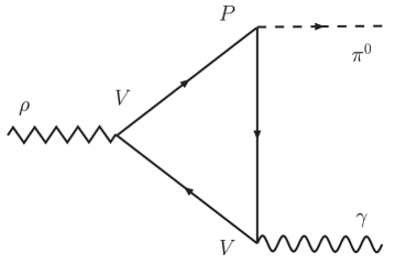
Figure 3: Two examples of the PVV triangle graphs where just one of the vector vertices couples to a photon, whereas the other couples to a vector meson. These two graphs describe the decays of $\omega$ and $\rho$ mesons into a photon and a pion.

$$|F_{m_{\pi}=0}(\pi^{0}\to 2\gamma)|=\frac{e^{2}}{4\pi^{2}f_{\pi}}=0.0251~{}\mbox{\rm GeV}^{-1}$$ (19)

very close to experimental data PDG2004

$$|F_{\rm exp}(\pi^{0}\to 2\gamma)|=\left[\frac{64\pi\Gamma(\pi^{0}\to\gamma\gamma)}{m_{\pi}^{3}}\right]^{1/2}=(0.0252\pm 0.0009)~{}\mbox{\rm GeV}^{-1}~{}.$$ (20)

Likewise, the $u$, $d$ quark triangles for $\rho\to\pi\gamma$ decay give Delbourgo

$$|F(\rho\to\pi\gamma)|=\frac{eg_{\rho}}{8\pi^{2}f_{\pi}}=0.206~{}\mbox{\rm GeV}^{-1}$$ (21)

for $g_{\rho}=4.965\pm 0.002$ found from $\rho^{0}\to e^{-}e^{+}$ decay PDG2004 :

$$\Gamma(\rho^{0}\to e^{-}e^{+})=\frac{e^{4}m_{\rho}}{12\pi g_{\rho}^{2}}=(7.02\pm 0.11)~{}\mbox{\rm keV}~{}.$$ (22)

The calculated $|F(\rho\to\pi\gamma)|$ is also near data PDG2004 ,

$$|F_{\rm exp}(\rho\to\pi\gamma)|=\left[\frac{12\pi\Gamma(\rho\to\pi\gamma)}{q^{3}}\right]^{1/2}=(0.225\pm 0.011)~{}\mbox{\rm GeV}^{-1}~{},$$ (23)

where $q=(m_{\rho}^{2}-m_{\pi}^{2})/(2m_{\rho})$ is the photon momentum. [Actually, the above value is a weighted average of $F_{\rm exp}(\rho^{0}\to\pi^{0}\gamma)$ and $F_{\rm exp}(\rho^{\pm}\to\pi^{\pm}\gamma)$ amplitudes.]

Next we predict the $u$, $d$ quark triangle amplitude for $\omega\to\pi\gamma$ taking $\omega$ as 99% nonstrange PDG2004 ($\cos^{2}\phi_{V}\approx 0.99$)

$$|F(\omega\to\pi\gamma)|=\frac{\cos\phi_{V}\,e\,g_{\omega}}{8\pi^{2}f_{\pi}}=0.705~{}\mbox{\rm GeV}^{-1}$$ (24)

for $g_{\omega}=17.06\pm 0.28$ found from $\omega\to e^{-}e^{+}$ decay. The mixing angle is

$$\phi_{V}=\theta_{V}-\arctan(\frac{1}{\sqrt{2}})=\arctan\sqrt{\frac{\frac{1}{3}(4m_{K^{\star}}^{2}-m_{\rho}^{2})-m_{\varphi}^{2}}{m_{\omega}^{2}-\frac{1}{3}(4m_{K^{\star}}^{2}-m_{\rho}^{2})}}-\arctan(\frac{1}{\sqrt{2}})=(5.208\pm 0.092)^{\circ}~{}.$$ (25)

Again this theory in Eq. (24) is near data $(0.722\pm 0.012)~{}\mbox{\rm GeV}^{-1}$ PDG2004 .

Other PVV photon decays involve the $\eta$ and $\eta^{\prime}$ mixed non–strange and $\bar{s}s$ pseudoscalar mesons. Again the quark triangle amplitudes are a close match with data Delbourgo ; delbourgo95 ; bramon98 .

The quark–triangle (QT) calculation gives reliable predictions also for the $\eta$ and $\eta^{\prime}$ two–photon decays:

$$|F(\eta\to\gamma\gamma)|=\frac{e^{2}}{4\pi^{2}f_{\pi}}\frac{N_{c}}{9}(5\cos\phi_{P}-\sqrt{2}\frac{\hat{m}}{m_{s}}\sin\phi_{P})=0.0255\mbox{\rm GeV}^{-1}~{},$$ (26)

$$|F(\eta^{\prime}\to\gamma\gamma)|=\frac{e^{2}}{4\pi^{2}f_{\pi}}\frac{N_{c}}{9}(5\sin\phi_{P}+\sqrt{2}\frac{\hat{m}}{m_{s}}\cos\phi_{P})=0.0345~{}\mbox{\rm GeV}^{-1}~{}.$$ (27)

This should be compared with the experimental data:

$$|F_{\rm exp}(\eta\to\gamma\gamma)|=\left[\frac{64\pi\Gamma(\eta\to\gamma\gamma)}{m_{\eta}^{3}}\right]^{1/2}=(0.02498\pm 0.00064)~{}\mbox{\rm GeV}^{-1}~{},$$ (28)

$$|F_{\rm exp}(\eta^{\prime}\to\gamma\gamma)|=\left[\frac{64\pi\Gamma(\eta^{\prime}\to\gamma\gamma)}{m_{\eta^{\prime}}^{3}}\right]^{1/2}=(0.03133\pm 0.00055)~{}\mbox{\rm GeV}^{-1}~{},$$ (29)

where $\Gamma(\eta\to\gamma\gamma)=(0.5108\pm 0.0268)~{}\mbox{\rm keV}$ and $\Gamma(\eta^{\prime}\to\gamma\gamma)=(4.29\pm 0.15)~{}\mbox{\rm keV}$. The ratio of the constituent quark masses is $m_{s}/m=2f_{K}/f_{\pi}-1=1.445\pm 0.024$ for $f_{\pi^{\pm}}=(92.4\pm 0.3)~{}\mbox{\rm MeV}$ and $f_{K}=(113.0\pm 1.0)~{}\mbox{\rm MeV}$ PDG2004 . The mixing angle is Jones:1979ez ; Kekez:2000aw

$$\phi_{P}=\theta_{P}+\arctan({\sqrt{2}})=\arctan\sqrt{\frac{(m_{\eta^{\prime}}^{2}-2m_{K}^{2}+m_{\pi}^{2})(m_{\eta}^{2}-m_{\pi}^{2})}{(2m_{K}^{2}-m_{\pi}^{2}-m_{\eta}^{2})(m_{\eta^{\prime}}^{2}-m_{\pi}^{2})}}=(42.441\pm 0.019)^{\circ}~{}.$$ (30)

Next, we can calculate the $\rho^{0}\to\eta\gamma$ amplitude employing the quark–triangle diagram,

$$|F(\rho^{0}\to\eta\gamma)|=\frac{eg_{\rho}}{8\pi^{2}f_{\pi}}3\cos\phi_{P}=0.456~{}\mbox{\rm GeV}^{-1}~{}.$$ (31)

Again, this is close to the experimental data,

$$|F_{\rm exp}(\rho^{0}\to\eta\gamma)|=\left[\frac{12\pi\Gamma(\rho^{0}\to\eta\gamma)}{q^{3}}\right]^{1/2}=(0.48\pm 0.03)~{}\mbox{\rm GeV}^{-1}~{},$$ (32)

where $q=(m_{\rho}^{2}-m_{\eta}^{2})/(2m_{\rho})=(194.5\pm 0.4)~{}\mbox{\rm MeV}$ is the photon momentum and $\Gamma(\rho^{0}\to\eta\gamma)=(45.1\pm 6.0)~{}\mbox{\rm keV}$. A similar situation is with the $\eta^{\prime}\to\rho\gamma$ amplitude, for which the quark–triangle calculation gives

$$|F(\eta^{\prime}\to\rho^{0}\gamma)|=\frac{eg_{\rho}}{8\pi^{2}f_{\pi}}3\sin\phi_{P}=0.417~{}\mbox{\rm GeV}^{-1}~{}.$$ (33)

The corresponding experimental value is

$$|F_{\rm exp}(\eta^{\prime}\to\rho^{0}\gamma)|=\left[\frac{4\pi\Gamma(\eta^{\prime}\to\rho^{0}\gamma)}{q^{3}}\right]^{1/2}=(0.411\pm 0.017)~{}\mbox{\rm GeV}^{-1}~{},$$ (34)

where $q=(m_{\eta^{\prime}}^{2}-m_{\rho}^{2})/(2m_{\eta^{\prime}})=(164.7\pm 0.4)~{}\mbox{\rm MeV}$ is the photon momentum and

$$\Gamma(\eta^{\prime}\to\rho^{0}\gamma\,\,\,\mbox{\rm including non--resonant}\,\,\,\pi^{+}\pi^{-}\gamma)=(60.0\pm 5.0)~{}\mbox{\rm keV}$$ (35)

is the experimental decay width PDG2004 .

The $\eta\to\pi\pi\gamma$ amplitude is

$$|M^{\mbox{\rm\scriptsize VMD}}_{\eta\to\pi\pi\gamma}|=|\frac{2g_{\rho\pi\pi}M^{\mbox{\rm\scriptsize QT}}_{\rho^{0}\to\eta\gamma}}{m_{\rho}^{2}-s}|=9.80~{}\mbox{\rm GeV}^{-3}$$ (36)

where $s=m_{\pi}^{2}$. The $\eta\to\pi\pi\gamma$ decay width is

$$\Gamma(\eta\to\pi\pi\gamma)=\frac{|M_{\eta\to\pi\pi\gamma}|^{2}}{(2\pi)^{3}}m_{\eta}^{7}Y_{\eta}=56.2~{}\mbox{\rm eV}~{},$$ (37)

where $Y_{\eta}=0.98\cdot 10^{-5}$ thew . This is in a good agreement with the experimental value

$$\Gamma(\eta\to\pi\pi\gamma)=(60.4\pm 3.6)~{}\mbox{\rm eV}~{},$$ (38)

revealing that the vector meson dominance is the main effect, while the coupling through VPPP quark box loop (“contact term”) contributes little.

It is known that $\omega\to 3\pi$ decay is dominated by $\rho$–meson poles. The required $\omega\to\rho\pi$ amplitude can be estimated as

$$|M^{\mbox{\rm\scriptsize VMD}}(\omega\to\rho\pi)|=\left(\frac{g_{\rho}}{e}\right)|F(\omega\to\pi^{0}\gamma)|\sim 12~{}\mbox{\rm GeV}^{-1}~{},$$ (39)

but cannot be measured because there is no phase space for this process. The $\omega\to\rho\pi$ amplitude is more precisely defined with QL, additionally enhanced with a meson loop associated with sigma exchange delbourgo95 ; bramon98 ; freund-nandi-rudaz ,

$$|M(\omega\to\rho\pi)|_{\mbox{\rm\scriptsize QT}}=\frac{3g_{\rho\pi\pi}^{2}}{8\pi^{2}f_{\pi}}\approx 15~{}\mbox{\rm GeV}^{-1}~{}.$$ (40)

The scalar amplitude $M^{\mbox{\rm\scriptsize VMD}}(\omega\to 3\pi)$ is dominated by the $\rho$ meson in each of the three possible channels gell-mann ,

$$|M^{\mbox{\rm\scriptsize VMD}}(\omega\to 3\pi)|=2g_{\rho\pi\pi}|M(\omega\to\rho\pi)|\left[\frac{1}{m_{\rho}^{2}-s}+\frac{1}{m_{\rho}^{2}-t}+\frac{1}{m_{\rho}^{2}-u}\right]\approx 1480~{}\mbox{\rm GeV}^{-3}~{}.$$ (41)

Following Thew’s phase space analysis thew , we get

$$\Gamma(\omega\to\ 3\pi)=\frac{|M^{\mbox{\rm\scriptsize VMD}}(\omega\to 3\pi)|^{2}}{(2\pi)^{3}}m_{\omega}^{7}Y_{\omega}=7.3~{}\mbox{\rm MeV}$$ (42)

where $Y_{\omega}=4.57\cdot 10^{-6}$ is used. The predicted value is close to the experimental value PDG2004

$$\Gamma(\omega\to 3\pi)=(7.6\pm 0.1)~{}\mbox{\rm MeV}~{}.$$ (43)

Here we have taken $\omega$ as pure NS, although it is about 99% NS, since $\phi_{V}=(5.208\pm 0.092)^{\circ}$ from our Eq. (25).

In the quark–level $\sigma$–model a quark box diagram contributes to the $\omega\to 3\pi$ decay. This box diagram can be interpreted as a contact term. It is shown that the contact contribution is small by itself, but can be enlarged through the interference effect lucio00 .

Using $\phi_{P}=(42.441\pm 0.019)^{\circ}$ from our Eq. (30), we predict the tensor $T\to PP$ branching ratios for $a_{2}(1320)$:

$$\begin{array}[]{ll}\mbox{\rm BR}(\frac{\textstyle{a_{2}\to\eta\pi}}{\textstyle{a_{2}\to K\bar{K}}})=\left(\frac{\textstyle{p_{\eta\pi}}}{\textstyle{p_{K}}}\right)^{5}2\cos^{2}\phi_{P}=2.996&(\mbox{\rm data}\,\,\,\,2.96\pm 0.54)~{},\\ \mbox{\rm BR}(\frac{\textstyle{a_{2}\to\eta^{\prime}\pi}}{\textstyle{a_{2}\to K\bar{K}}})=\left(\frac{\textstyle{p_{\eta^{\prime}\pi}}}{\textstyle{p_{K}}}\right)^{5}2\sin^{2}\phi_{P}=0.1113&(\mbox{\rm data}\,\,\,\,0.108\pm 0.025)~{},\\ \mbox{\rm BR}(\frac{\textstyle{a_{2}\to\eta^{\prime}\pi}}{\textstyle{a_{2}\to\eta\pi}})=\left(\frac{\textstyle{p_{\eta^{\prime}\pi}}}{\textstyle{p_{\eta\pi}}}\right)^{5}\tan^{2}\phi_{P}=0.0371&(\mbox{\rm data}\,\,\,\,0.0366\pm 0.0069)~{},\end{array}$$ (47)

for center of mass momenta $p_{\eta\pi}=535~{}\mbox{\rm MeV}$, $p_{\eta^{\prime}\pi}=287~{}\mbox{\rm MeV}$, $p_{K}=437~{}\mbox{\rm MeV}$. The above data branching ratios follow from $a_{2}(1320)$ recent fractions PDG2004 : $\mbox{\rm BR}(a_{2}\to\eta\pi)=(14.5\pm 1.2)\%$, $\mbox{\rm BR}(a_{2}\to K\bar{K})=(4.9\pm 0.8)\%$ and $\mbox{\rm BR}(a_{2}\to\eta^{\prime}\pi)=(5.3\pm 0.9)\cdot 10^{-3}$.

4 Comments related to the gluon anomaly

The approach using the pseudoscalar coupling is, in our opinion, also relevant for the effects related to the non-Abelian, “gluon” ABJ axial anomaly. Here, we comment on this only briefly, and direct the reader to the original references for details.

4.1 Goldstone structure and $\eta$-$\eta^{\prime}$ phenomenology

The first point concerns the $\eta$-$\eta^{\prime}$ complex and the $U_{A}(1)$ problem related to it.

In the chiral limit $m_{\pi}=m_{K}=m_{\eta_{8}}=0$, since all members of the flavor-SU(3) pseudoscalar meson octet are massless in this theoretical, but very useful limit. The only non-vanishing ground-state pseudoscalar meson mass in this limit is the mass of the SU(3)-singlet pseudoscalar meson $\eta_{1}$. This is thanks to the non-Abelian, gluon ABJ axial anomaly, i.e., to the fact that the divergence of the SU(3)-singlet axial current

$$A^{\mu}_{0}(x)=\overline{\Psi}(x)\gamma^{\mu}\gamma_{5}\Psi(x)\,,$$ (48)

receives the contributions from gluon fields $G_{a}^{\mu\nu}$ similar to those of photon fields $F^{\mu\nu}$ in Eq. (17), namely

$$\partial_{\mu}A^{\mu}_{0}=2{\rm i}m_{u}\,\overline{u}\gamma_{5}u+2{\rm i}m_{d}\,\overline{d}\gamma_{5}d+2{\rm i}m_{s}\,\overline{s}\gamma_{5}s+\frac{3\,g^{2}}{32\pi^{2}}\epsilon_{\mu\nu\alpha\beta}G_{a}^{\mu\nu}G_{a}^{\alpha\beta}\,.$$ (49)

This removes the $U_{A}(1)$ symmetry and explains why only eight pseudoscalar mesons are light, and not nine; i.e., why there is an octet of (almost-)Goldstone bosons, but not a nonet. The physically observed $\eta$ and $\eta^{\prime}$ are then the mixtures of the anomalously heavy $\eta_{1}$ and (almost-)Goldstone $\eta_{8}$ in such a way that $\eta^{\prime}$ is predominantly $\eta_{1}$ and $\eta$ is predominantly $\eta_{8}$. This is how the gluon anomaly can save us from the $U_{A}(1)$ problem in principle, and the details of how we achieve a successful description of the $\eta$-$\eta^{\prime}$ complex, are given in the references Jones:1979ez ; Kekez:2000aw ; Klabucar:1997zi ; Klabucar:2000me ; Klabucar:2001gr . Here we just sketch some important points. The mass matrix squared $\hat{M}^{2}$ in the quark basis $|u\bar{u}\rangle$, $|d\bar{d}\rangle$, $|s\bar{s}\rangle$ is

$$\hat{M}^{2}=\hat{M}_{\mbox{\rm\scriptsize NA}}^{2}+\hat{M}_{\rm A}^{2}=\left[\begin{array}[]{ccc}m_{u\bar{u}}^{2}&0&0\\ 0&m_{d\bar{d}}^{2}&0\\ 0&0&m_{s\bar{s}}^{2}\end{array}\right]+\beta\left[\begin{array}[]{ccl}1&1&X\\ 1&1&X\\ X&X&X^{2}\end{array}\right]~{},$$ (50)

where $\hat{M}_{\mbox{\rm\scriptsize NA}}^{2}$ is the non-anomalous part of the matrix, since $m_{u\bar{u}}^{2}=m_{d\bar{d}}^{2}=m_{\pi}^{2}$ and $m_{s\bar{s}}^{2}=2m_{K}^{2}-m_{\pi}^{2}$ would be the masses of the respective “non-strange” (NS) and “strange” (S) $q\bar{q}$ mesons if there were no gluon anomaly. In the NS sector, in the isospin symmetry limit (which is very close to reality), the relevant combinations are $|\pi^{0}\rangle=|u\bar{u}-d\bar{d}\rangle/\sqrt{2}$ as the neutral partner of the charged pions $|\pi^{\pm}\rangle$ in the isospin 1 triplet, and the isospin 0 combination $|u\bar{u}+d\bar{d}\rangle/\sqrt{2}$. In the absence of gluon anomaly, but with an $s$-quark mass heavier than the isosymmetric $u$ and $d$ ones, $\eta$ would reduce to $|{\rm NS}\rangle=|u\bar{u}+d\bar{d}\rangle/\sqrt{2}$ with the mass $m_{\mbox{\rm\scriptsize NS}}=m_{\pi}$, and $\eta^{\prime}$ to $|{\rm S}\rangle=|s\bar{s}\rangle$ with the mass $m_{\mbox{\rm\scriptsize S}}=m_{s\bar{s}}$. Both of these assignments are in conflict with experiment. The realistic contributions of various flavors to $\eta$ and $\eta^{\prime}$ and their masses (i.e., the realistic $\eta$-$\eta^{\prime}$ mixing) are obtained only thanks to $\hat{M}_{\rm A}^{2}$, the anomalous contribution to the mass matrix. In $\hat{M}_{\rm A}^{2}$, the quantity $\beta$ describes transitions $|q\bar{q}\rangle\to|q^{\prime}\bar{q}^{\prime}\rangle$ ($q,q^{\prime}=u,d,s$) due to the gluon anomaly and $X$ describes the effects of the SU(3) flavor symmetry breaking on these transitions. In Refs. Jones:1979ez ; Kekez:2000aw ; Klabucar:2000me , as the first step in solving the $U_{A}(1)$ problem, we extract $\eta_{8}$, $\eta_{1}$ masses from the $\eta$, $\eta^{\prime}$ via

$$m_{\eta_{8}}^{2}=(m_{\eta}\cos\theta_{P})^{2}+(m_{\eta^{\prime}}\sin\theta_{P})^{2}=(572.73~{}\mbox{\rm MeV})^{2}~{},$$ (51)

$$m_{\eta_{1}}^{2}=(m_{\eta}\sin\theta_{P})^{2}+(m_{\eta^{\prime}}\cos\theta_{P})^{2}=(943.05~{}\mbox{\rm MeV})^{2}~{},$$ (52)

where $\theta_{P}=\phi_{P}-\arctan(\sqrt{2})=(-12.295\pm 0.019)^{\circ}$. The mesons $\eta_{8}$ and $\eta_{1}$ are defined as

$$|\eta_{8}\rangle = \frac{1}{\sqrt{6}}(|u\bar{u}\rangle+|d\bar{d}\rangle-2|s\bar{s}\rangle)~{},$$ (53)

$$|\eta_{1}\rangle = \frac{1}{\sqrt{3}}(|u\bar{u}\rangle+|d\bar{d}\rangle+|s\bar{s}\rangle)~{}.$$ (54)

The $\eta_{8}$ meson mass (51) $m_{\eta_{8}}=572.73~{}\mbox{\rm MeV}$ is 4.56% greater than the observed PDG2004 $m_{\eta}=(547.75\pm 0.12)~{}\mbox{\rm MeV}$. The singlet $\eta_{1}$ mass (52) $m_{\eta_{1}}=943.06~{}\mbox{\rm MeV}$ is only 1.56% below the observed $m_{\eta}^{\prime}=(957.78\pm 0.14)~{}\mbox{\rm MeV}$ and close to the nonstrange–$\bar{s}s$ mixing $U_{A}(1)$ mass dictated by phenomenology Jones:1979ez ; Kekez:2000aw ; Klabucar:2000me

$$m_{U_{A}(1)}\equiv(3\beta)^{1/2}=\left[\frac{3}{4}\frac{(m_{\eta^{\prime}}^{2}-m_{\pi}^{2})(m_{\eta}^{2}-m_{\pi}^{2})}{m_{K}^{2}-m_{\pi}^{2}}\right]^{1/2}=915.31~{}\mbox{\rm MeV}~{},$$ (55)

(This is also close to $912~{}\mbox{\rm MeV}$, which is the mass found in the analogous DS approach Kekez:2000aw ; Klabucar:2000me .)

We call the quantity (55) the “mixing $U_{A}(1)$ mass” since the mass matrix (which is especially clear in the nonstrange-strange quark basis) reveals that $m_{U_{A}(1)}$ induces the mixing between the nonstrange isoscalar $(|\bar{u}u\rangle+|\bar{d}d\rangle/\sqrt{2}$ and $\bar{s}s$ quark-antiquark states. Equivalently, $m_{U_{A}(1)}$ can be viewed as being generated by the transitions among the $\bar{u}u$, $\bar{d}d$ and $\bar{s}s$ pseudoscalar states; via quark loops, these pseudoscalar $\bar{q}q$ bound states can annihilate into gluons which in turn via another quark loop can again recombine into another pseudoscalar $\bar{q}^{\prime}q^{\prime}$ bound state of the same or different flavor. The quantity $\beta$ appearing in Eq. (55) is then the annihilation strength of such transitions, in the limit of an exact SU(3) flavor symmetry. (The realistic breaking of this symmetry is easily introduced and improves our description of the $\eta$-$\eta^{\prime}$ complex considerably.) The “diamond” graph in Fig. 4 gives just the simplest example of such an annihilation/recombination transition. Since these annihilations occur in the nonperturbative regime of QCD, all graphs with any even number of gluons instead of just those two in Fig. 4, can be just as significant in annihilating and forming a $C^{+}$ pseudoscalar $\bar{q}q$ meson. Indeed, this nonperturbative $U_{A}(1)$ mass scale, Eq. (55), is still 3 times higher than the gluon “diamond” graph evaluated perturbatively Choudhury . Thus, we cannot calculate $\beta=m_{U_{A}(1)}^{2}/3$ and the situation is much more complicated and less clear than in the Abelian case, where we have seen, in Sec. 2.C, that PVV, the quark triangle graph with pseudoscalar coupling, reproduces the effect of the axial anomaly, i.e., the WZ Lagrangian term, or equivalently, the effect of the anomalous term $({e^{2}N_{c}}/{16\pi^{2}})\mbox{\rm tr}(\tau_{3}{\cal Q}^{2})\epsilon_{\mu\nu\alpha\beta}F^{\mu\nu}F^{\alpha\beta}$ in the divergence (17) of the current $A^{\mu}_{3}(x)$. Can it then be founded to think that the annihilation graphs with the pseudoscalar meson-quark coupling, such as the “diamond” graph in Fig. 4, give rise to the anomalous term $({3\,g^{2}}/{32\pi^{2}})\epsilon_{\mu\nu\alpha\beta}G_{a}^{\mu\nu}G_{a}^{\alpha\beta}$ in the divergence (49) of the SU(3)-singlet current $A^{\mu}_{0}(x)$, and thus ultimately to the large mass of $\eta_{0}$ (and of the observed $\eta^{\prime}$)? Well, this conjecture may remain a speculation since we cannot calculate $\beta$ due to the nonperturbative nature of the problem. Nevertheless, when we use it in our approach as a parameter with the value given by Eq. (55), we obtain a very good description of the $\eta$-$\eta^{\prime}$ complex phenomenology Jones:1979ez ; Kekez:2000aw ; Klabucar:1997zi ; Klabucar:2000me ; Klabucar:2001gr . This includes not only the masses of $\eta$ and $\eta^{\prime}$, but also their $\gamma\gamma$ decay widths, and the mixing angle $\theta_{P}\approx-13^{\circ}$ consistently following from the masses and $\gamma\gamma$ widths. This gives a strong motivation for the above conjecture.

Figure 4: Nonperturbative QCD annihilation of a quark-antiquark bound state illustrated by the diagram with two-gluon exchange. The $\bar{q}q$ pseudoscalar $P$ is coupled to a quark loop, whereby it can annihilate into gluons which in turn recombine into the pseudoscalar $P^{\prime}$ having the flavor content $\bar{q^{\prime}}q^{\prime}$.

4.2 Taming of strong CP problem

We should also note that our conjecture in the previous subsection goes well with the arguments of Banerjee et al. Mitra , that there is really no strong CP problem. They find that one does not need vanishing $\Theta_{\rm eff}=\Theta-{\rm tr}\ln{\hat{M}}$ (where ${\hat{M}}$ is the quark mass matrix). Thus, one does not need any fine-tuning, and all CP violation in the QCD Lagrangian can be avoided by having $\Theta=0$ in its CP-violating term

$${\cal L}_{\Theta}=-\Theta\,\frac{g^{2}}{64\pi^{2}}\epsilon_{\mu\nu\alpha\beta}G_{a}^{\mu\nu}G_{a}^{\alpha\beta}\,.$$ (56)

This term in the QCD Lagrangian breaks the $U_{A}(1)$ symmetry and corresponds to the anomalous term $\propto\epsilon_{\mu\nu\alpha\beta}G_{a}^{\mu\nu}G_{a}^{\alpha\beta}$ in the divergence (49) of the singlet current. The term (56) is allowed by gauge invariance and renormalizability, but apparent nonexistence of the strong CP violation, and also of axions, is the solid reason to have it vanishing. Our conjecture, that P-coupled annihilation graphs reproduce the effect of the gluon ABJ anomaly, naturally agrees with the vanishing of this term and with putting the case of the strong CP problem to rest à la Banerjee et al. Mitra .

5 Summary/Discussion

We have presented and surveyed in detail the method of pseudoscalar coupling of pseudoscalar mesons to the “triangle” and “box” quark loops. We have reviewed how this method gives the equivalent results to the anomaly calculations. The P-coupling method has also been illustrated on the example of many decay amplitudes.

The AVV anomaly Adler69 ; BellJackiw69 involves 10 invariant amplitudes (reduced to 1 or 2 amplitudes for $\pi^{0}\to\gamma\gamma$ decay using additional Ward identities). If instead one considers the PVV transition with a pseudoscalar coupling, then the PVV quark triangle amplitude is finite and leads to many decay amplitudes (over 15) then in agreement with data to within 3% and not involving free parameters Delbourgo . To solve instead the former AVV decay problem, very light axion bosons have been predicted but have not yet been observed PDG2004 .

Also, there is the $U_{A}(1)$ and $\Theta$ problem involving gluons whereby strong interaction QCD leads to CP violation, definitely a “strong CP problem” because CP violation is known to occur at the $10^{-3}$ weak interaction amplitude level PDG2004 . Physicists have tried to circumvent this “$U_{A}(1)$ – strong CP problem” either via the topology of gauge fields or by investigating the $\Theta$–vacuum for this strong CP problem Mitra .

In this paper we have circumvented the need to deal directly with the above photon or gluon AVV anomalies by studying instead (finite) PVV quark triangle graphs. Then we have given our phenomenological results – which always are in approximate agreement with the data. Next we return to the $U_{A}(1)$ problem and again use quark triangle diagrams coupled to 2 gluons. Invoking nonstrange–strange particle mixing, the predicted $U_{A}(1)$ mass is within 3% of data Jones:1979ez ; Kekez:2000aw ; Klabucar:2000me .

Thus we circumvent both photon and, admittedly on a much more speculative level, also the gluon ABJ anomaly without resorting either to unmeasured axions or to a strong CP violating term in the QCD Lagrangian.

References

- (1) S. L. Adler, Phys. Rev. 177 (1969) 2426.
- (2) J. S. Bell and R. Jackiw, Nouvo Cim. A 60 (1969) 47.
- (3) See, for example, Ref. Georgi:1985kw by H. Georgi, and Chap. 5 of its updated version available in electronic form at http://schwinger.harvard.edu/~georgi/weak5.ps.
- (4) H. Georgi, “Weak Interactions And Modern Particle Theory”, Menlo Park, USA: Benjamin/Cummings (1984).
- (5) J. Wess and B. Zumino, Phys. Lett. B 37 (1971) 95.
- (6) J. Steinberger, Phys. Rev. 76 (1949) 1180.
- (7) R. Alkofer and L. von Smekal, Phys. Rept. 353 (2001) 281 [arXiv:hep-ph/0007355].
- (8) P. Maris and C.D. Roberts, Int. J. Mod. Phys. E 12 (2003) 297 [arXiv:nucl-th/0301049].
- (9) R. Delbourgo, Dongsheng Liu and M. D. Scadron, Int. J. Mod. Phys. A 14 (1999) 4331 [arXiv:hep-ph/9905501]; M. D. Scadron, F. Kleefeld, G. Rupp and E. van Beveren, Nucl. Phys. A 724 (2003) 391 [hep-ph/0211275].
- (10) R. Delbourgo and M. D. Scadron, Mod. Phys. Lett. A 10 (1995) 251 [arXiv:hep-ph/9910242].
- (11) A. Bramon, Riazuddin and M. D. Scadron, J. Phys. G 24 (1998) 1 [arXiv:hep-ph/9709274].
- (12) S. Eidelman et al., Phys. Lett. B 592 (2004) 1.
- (13) H. Banerjee, D. Chatterjee and P. Mitra, Phys. Lett. B 573 (2003) 109 [arXiv:hep-ph/0012284].
- (14) S. L. Adler, B. W. Lee, S. Treiman and A. Zee, Phys. Rev. D 4 (1971) 3497; M. V. Terent’ev, Phys. Lett. 38B (1972) 419; R. Aviv and A. Zee, Phys. Rev. D 5 (1972) 2372.
- (15) T. Hakioglu and M. D. Scadron, Phys. Rev. D 42 (1990) 941; T. Hakioglu and M. D. Scadron, Phys. Rev. D 43 (1991) 2439.
- (16) A. A. Andrianov, D. Espriu and R. Tarrach, Nucl. Phys. B 533 (1998) 429.
- (17) Ll. Ametller, L. Bergström, A. Bramon and E. Massó, Nucl. Phys. B 228 (1983) 301.
- (18) B. Bistrović and D. Klabučar, Phys. Rev. D 61 (2000) 033006 [arXiv:hep-ph/9907515].
- (19) D. Kekez, B. Bistrović and D. Klabučar, Int. J. Mod. Phys. A 14 (1999) 161 [arXiv:hep-ph/9809245].
- (20) C.D. Roberts, Nucl. Phys. A 605 (1996) 475; C.D. Roberts, in: Chiral Dynamics: Theory and Experiment, eds. A. M. Bernstein and B. R. Holstein, Lecture Notes in Physics, Vol. 452, Springer, Berlin, 1995 p. 68.
- (21) M. Bando, M. Harada and T. Kugo, Prog. Theor. Phys. 91 (1994) 927 [arXiv:hep-ph/9312343].
- (22) R. Alkofer and C. D. Roberts, Phys. Lett. B 369 (1996) 101 [arXiv:hep-ph/9510284 ].
- (23) B. Bistrović and D. Klabučar, Phys. Lett. B 478 (2000) 127 [arXiv:hep-ph/9912452].
- (24) D. Kekez and D. Klabučar, Phys. Lett. B 387 (1996) 14 [arXiv:hep-ph/9605219].
- (25) D. Klabučar and D. Kekez, Phys. Rev. D 58 (1998) 096003 [arXiv:hep-ph/9710206].
- (26) D. Kekez and D. Klabučar, Phys. Lett. B 457 (1999) 359 [arXiv:hep-ph/9812495].
- (27) D. Kekez and D. Klabucar, Phys. Rev. D 71 (2005) 014004 [arXiv:hep-ph/0307110].
- (28) J. S. Ball and T.-W. Chiu, Phys. Rev. D 22 (1980) 2542.
- (29) Yu. M. Antipov et al., Phys. Rev. D 36 (1987) 21.
- (30) M. A. Moinester, V. Steiner and S. Prakhov, Hadron-Photon Interactions in COMPASS, to be published in the proceedings of 37th International Winter Meeting on Nuclear Physics, Bormio, Italy, 25-29 Jan 1999, [arXiv:hep-ex/9903017].
- (31) R. A. Miskimen, K. Wang and A. Yagneswaran (spokesmen), Study of the Axial Anomaly using the Reaction Near Threshold, Letter of intent, CEBAF-experiment 94-015.
- (32) D. Klabučar and B. Bistrović, arXiv:hep-ph/0009259.
- (33) D. Klabučar and B. Bistrović, arXiv:hep-ph/0012273.
- (34) D. G. Sutherland, Nucl. Phys. B 2 (1967) 433.
- (35) M. Veltman, Proc. R. Soc. London A301, 107 (1967).
- (36) Besides original references, some may also find helpful more pedagogical presentations such as that in Ref. Yndurain:1999ui .
- (37) H. Georgi, Chapter 6a (available at http://schwinger.harvard.edu/ georgi/weak6a.ps) of the updated version of the monograph Georgi:1985kw on weak interactions.
- (38) K. Hagiwara et al., Phys. Rev. D 66, 010001 (2002).
- (39) D. Kekez, D. Klabučar and M. D. Scadron, J. Phys. G 26 (2000) 1335 [arXiv:hep-ph/0003234].
- (40) H. F. Jones and M. D. Scadron, Nucl. Phys. B 155 (1979) 409.
- (41) R. L. Thews, Phys. Rev. D 10 (1974) 2993.
- (42) P. G. O. Freund and S. Nandi, Phys. Rev. Lett. 32 (1974) 181; S. Rudaz, Phys. Lett. B 145 (1984) 281.
- (43) M. Gell-Mann, D. Sharp and W. Wagner, Phys. Rev. Lett. 8 (1962) 261.
- (44) J. L. Lucio, M. Napsuciale, M. D. Scadron and V. M. Villanueva, Phys. Rev. D 61 (2000) 034013.
- (45) D. Klabučar and D. Kekez, Phys. Rev. D 58, 096003 (1998) [arXiv:hep-ph/9710206].
- (46) D. Klabučar, D. Kekez and M. D. Scadron, arXiv:hep-ph/0012267.
- (47) D. Kekez, D. Klabučar and M. D. Scadron, J. Phys. G 27 (2001) 1775 [arXiv:hep-ph/0101324].
- (48) S. R. Choudhury and M. D. Scadron, Mod. Phys. Lett. A 1 (1986) 535.
- (49) F. J. Yndurain, “The theory of quark and gluon interactions,” New York, Berlin, Heidelberg, Tokyo: Springer-Verlag (1993).