Disentangling two- and four-quark state pictures of the charmed scalar mesons

Abstract

We suggest that the recently observed charmed scalar mesons $D_{0}^{0}(2308)$ (BELLE) and $D_{0}^{0,+}(2405)$ (FOCUS) are considered as different resonances. Using the QCD sum rule approach we investigate the possible four-quark structure of these mesons and also of the very narrow $D_{sJ}^{+}(2317)$, firstly observed by BABAR. We use diquak-antidiquark currents and work to the order of $m_{s}$ in full QCD, without relying on $1/m_{c}$ expansion. Our results indicate that a four-quark structure is acceptable for the resonances observed by BELLE and BABAR: $D_{0}^{0}(2308)$ and $D_{sJ}^{+}(2317)$ respectively, but not for the resonances observed by FOCUS: $D_{0}^{0,+}(2405)$.

Recently the first observations of the scalar charmed mesons have been reported. The very narrow $D_{sJ}^{+}(2317)$ was first discovered in the $D_{s}^{+}\pi^{0}$ channel by the BABAR Collaboration babar and its existence was confirmed by CLEO cleo , BELLE belle1 and FOCUS focus Collaborations. Its mass was commonly measured as $2317\nobreak\,\mbox{MeV}$, which is approximately $160\nobreak\,\mbox{MeV}$ below the prediction of the very successful quark model for the charmed mesons god . The BELLE Collaboration belle2 has also reported the observation of a rather broad scalar meson $D_{0}^{0}(2308)$, and the FOCUS Collaboration focus2 reported evidence for broad structures in both neutral and charged final states that, if interpreted as resonances in the $J^{P}=0^{+}$ channel, would be the $D_{0}^{0}(2407)$ and the $D_{0}^{+}(2403)$ mesons. While the mass of the scalar meson, $D_{0}^{0}(2308)$, observed by BELLE Collaboration is also bellow the prediction of ref. god (approximately $100\nobreak\,\mbox{MeV}$), the masses of the states observed by FOCUS Collaboration are in complete agreement with ref. god .

Due to its low mass, the structure of the meson $D_{sJ}^{+}(2317)$ has been extensively debated. It has been interpreted as a $c\bar{s}$ state dhlz ; bali ; ukqcd ; ht ; nari , two-meson molecular state bcl ; szc , $D-K$- mixing br , four-quark states ch ; tera ; mppr or a mixture between two-meson and four-quark states bpp . The same analyses would also apply to the meson $D_{0}^{0}(2308)$.

In the light sector the idea that the scalar mesons could be four-quark bound states is not new jaffe and, therefore, it is natural to consider analogous states in the charm sector.

We propose that the resonances observed by BELLE belle2 and FOCUS focus2 Collaborations be considered as two different resonances. In this work we use the method of QCD sum rules (QCDSR) svz to study the two-point functions of the scalar mesons, $D_{sJ}(2317)$, $D_{0}(2308)$ and $D_{0}(2405)$ considered as four-quark states. The use of the QCD sum rules to study the charmed scalar mesons was already done in refs. dhlz ; ht ; nari , but in these calculations they were interpreted as two-quark states.

In a recent calculation sca some of us have considered that the lowest lying scalar mesons are $S$-wave bound states of a diquark-antidiquark pair. As suggested in ref. jawil the diquark was taken to be a spin zero colour anti-triplet. We extend this prescription to the charm sector and, therefore, the corresponding interpolating fields containing zero, one and two strange quarks are:

$$j_{0} = \epsilon_{abc}\epsilon_{dec}(q_{a}^{T}C\gamma_{5}c_{b})(\bar{u}_{d}\gamma_{5}C\bar{d}_{e}^{T}),$$

$$j_{s} = {\epsilon_{abc}\epsilon_{dec}\over\sqrt{2}}\left[(u_{a}^{T}C\gamma_{5}c_{b})(\bar{u}_{d}\gamma_{5}C\bar{s}_{e}^{T})+u\leftrightarrow d\right],$$

$$j_{ss} = \epsilon_{abc}\epsilon_{dec}(s_{a}^{T}C\gamma_{5}c_{b})(\bar{q}_{d}\gamma_{5}C\bar{s}_{e}^{T}),$$ (1)

where $a,~{}b,~{}c,~{}...$ are colour indices, $C$ is the charge conjugation matrix and $q$ represents the quark $u$ or $d$ according to the charge of the meson. Since $D_{sJ}$ has one $\bar{s}$ quark, we choose the $j_{s}$ current to have the same quantum numbers of $D_{sJ}$, which is supposed to be an isoscalar. However, since we are working in the SU(2) limit, the isoscalar and isovector states are mass degenerate and, therefore, this particular choice has no relevance here.

The QCDSR for the charmed scalar mesons are constructed from the two-point correlation function

$$\Pi(q)=i\int d^{4}x~{}e^{iq.x}\langle 0|T[j_{S}(x)j^{\dagger}_{S}(0)]|0\rangle.$$ (2)

The coupling of the scalar meson, $S$, to the scalar current, $j_{S}$, can be parametrized in terms of the meson decay constant $f_{S}$ as sca : $\langle 0|j_{S}|S\rangle=\sqrt{2}f_{S}m_{S}^{4}$, therefore, the phenomenological side of Eq. (2) can be written as

$$\Pi^{phen}(q^{2})={2f_{S}^{2}m_{S}^{8}\over m_{S}^{2}-q^{2}}+\cdots\;,$$ (3)

where the dots denote higher resonance contributions that will be parametrized, as usual, through the introduction of the continuum threshold parameter $s_{0}$ io1 .

In the OPE side we work at leading order and consider condensates up to dimension six. We deal with the strange quark as a light one and consider the diagrams up to order $m_{s}$. To keep the charm quark mass finite, we use the momentum-space expression for the charm quark propagator. We follow ref. su and calculate the light quark part of the correlation function in the coordinate-space, which is then Fourier transformed to the momentum space in $D$ dimensions. The resulting light-quark part is combined with the charm-quark part before it is dimensionally regularized at $D=4$.

We can write the correlation function in the OPE side in terms of a dispersion relation:

$$\Pi^{OPE}(q^{2})=\int_{m_{c}^{2}}^{\infty}ds{\rho(s)\over s-q^{2}}\;,$$ (4)

where the spectral density is given by the imaginary part of the correlation function: $\rho(s)={1\over\pi}\mbox{Im}[\Pi^{OPE}(s)]$. After making a Borel transform on both sides, and transferring the continuum contribution to the OPE side, the sum rule for the scalar meson $S$ can be written as

$$2f_{S}^{2}m_{S}^{8}e^{-m_{S}^{2}/M^{2}}=\int_{m_{c}^{2}}^{s_{0}}ds~{}e^{-s/M^{2}}~{}\rho_{S}(s)\;,$$ (5)

where $\rho_{S}(s)=\rho^{pert}(s)+\rho^{m_{s}}(s)+\rho^{\langle\bar{q}q\rangle}(s)+\rho^{\langle G^{2}\rangle}(s)+\rho^{mix}(s)+\rho^{\langle\bar{q}q\rangle^{2}}(s)+\rho^{\langle G^{3}\rangle}(s)$, with

$$\rho^{pert}(s)={1\over 2^{10}3\pi^{6}}\int_{\Lambda}^{1}d\alpha\left({1-\alpha\over\alpha}\right)^{3}(m_{c}^{2}-s\alpha)^{4},$$ (6)

$$\rho^{\langle G^{2}\rangle}(s) = {\langle g^{2}G^{2}\rangle\over 2^{10}\pi^{6}}\int_{\Lambda}^{1}d\alpha~{}(m_{c}^{2}-s\alpha)\left[{m_{c}^{2}\over 9}\left({1-\alpha\over\alpha}\right)^{3}+\right.$$ (7)

$$+ \left.(m_{c}^{2}-s\alpha)\left({1-\alpha\over 2\alpha}+{(1-\alpha)^{2}\over 4\alpha^{2}}\right)\right],$$

$$\rho^{\langle G^{3}\rangle}(s)={\langle g^{3}G^{3}\rangle\over 2^{12}9\pi^{6}}\int_{\Lambda}^{1}d\alpha\left({1-\alpha\over\alpha}\right)^{3}(3m_{c}^{2}-s\alpha),$$ (8)

which are common to all three resonances and where the lower limit of the integrations is given by $\Lambda=m_{c}^{2}/s$. From $j_{0}$ we get: $\rho^{m_{s}}(s)=0$,

$$\rho^{\langle\bar{q}q\rangle}(s)=-{m_{c}\langle\bar{q}q\rangle\over 2^{6}\pi^{4}}\int_{\Lambda}^{1}d\alpha\left({1-\alpha\over\alpha}\right)^{2}(m_{c}^{2}-s\alpha)^{2},$$ (9)

$$\rho^{mix}(s) = {m_{c}\langle\bar{q}g\sigma.Gq\rangle\over 2^{6}\pi^{4}}\bigg{[}{1\over 2}\int_{\Lambda}^{1}d\alpha\left({1-\alpha\over\alpha}\right)^{2}(m_{c}^{2}-s\alpha)+$$ (10)

$$- \int_{\Lambda}^{1}d\alpha{1-\alpha\over\alpha}(m_{c}^{2}-s\alpha)\bigg{]},$$

$$\rho^{\langle\bar{q}q\rangle^{2}}(s)=-{\langle\bar{q}q\rangle^{2}\over 12\pi^{2}}\int_{\Lambda}^{1}d\alpha~{}(m_{c}^{2}-s\alpha).$$ (11)

From $j_{s}$ we get: $\rho^{m_{s}}(s)=0$,

$$\rho^{\langle\bar{q}q\rangle}(s)={1\over 2^{6}\pi^{4}}\int_{\Lambda}^{1}d\alpha~{}{1-\alpha\over\alpha}(m_{c}^{2}-s\alpha)^{2}\bigg{[}$$

$$-\langle\bar{q}q\rangle\left(2m_{s}+m_{c}{1-\alpha\over\alpha}\right)+m_{s}\langle\bar{s}s\rangle\bigg{]},$$ (12)

$$\rho^{mix}(s) = {1\over 2^{6}\pi^{4}}\int_{\Lambda}^{1}d\alpha~{}(m_{c}^{2}-s\alpha)\bigg{[}-{m_{s}\langle\bar{s}g\sigma.Gs\rangle\over 6}$$ (13)

$$+ \langle\bar{q}g\sigma.Gq\rangle\bigg{(}-m_{s}(1-\ln(1-\alpha))$$

$$- m_{c}{1-\alpha\over\alpha}\left(1-{1-\alpha\over 2\alpha}\right)\bigg{)}\bigg{]}$$

$$\rho^{\langle\bar{q}q\rangle^{2}}(s)=-{\langle\bar{q}q\rangle\langle\bar{s}s\rangle\over 12\pi^{2}}\int_{\Lambda}^{1}d\alpha~{}(m_{c}^{2}-s\alpha).$$ (14)

Finally from $j_{ss}$ we get

$$\rho^{m_{s}}(s)=-{m_{s}m_{c}\over 2^{8}3\pi^{6}}\int_{\Lambda}^{1}d\alpha\left({1-\alpha\over\alpha}\right)^{3}(m_{c}^{2}-s\alpha)^{3},$$ (15)

$$\rho^{\langle\bar{q}q\rangle}(s)={1\over 2^{6}\pi^{4}}\int_{\Lambda}^{1}d\alpha{1-\alpha\over\alpha}(m_{c}^{2}-s\alpha)^{2}\bigg{[}$$

$$\langle\bar{s}s\rangle\left(2m_{s}-m_{c}{1-\alpha\over\alpha}\right)-2m_{s}\langle\bar{q}q\rangle\bigg{]},$$ (16)

$$\rho^{mix}(s) = {1\over 2^{6}\pi^{4}}\int_{\Lambda}^{1}d\alpha~{}(m_{c}^{2}-s\alpha)\bigg{[}{\langle\bar{s}g\sigma.Gs\rangle\over 2}\bigg{(}{m_{s}\over 3}$$ (17)

$$- m_{s}{1-\alpha\over\alpha}-m_{c}{1-\alpha\over\alpha}\left(1-{1-\alpha\over 2\alpha}\right)\bigg{)}$$

$$- m_{s}\langle\bar{q}g\sigma.Gq\rangle(1-\ln(1-\alpha))\bigg{]},$$

$$\rho^{\langle\bar{q}q\rangle^{2}}(s)=-{\langle\bar{q}q\rangle\langle\bar{s}s\rangle\over 12\pi^{2}}\int_{\Lambda}^{1}d\alpha~{}(m_{c}^{2}-s\alpha).$$ (18)

For the charm quark propagator with two and three gluons attached we use the momentum-space expressions given in ref. rry .

In order to get rid of the meson decay constant and extract the resonance mass, $m_{S}$, we first take the derivative of Eq. (5) with respect to $1/M^{2}$ and then we divide it by Eq. (5) to get

$$m_{S}^{2}={\int_{m_{c}^{2}}^{s_{0}}ds~{}e^{-s/M^{2}}~{}s~{}\rho_{S}(s)\over\int_{m_{c}^{2}}^{s_{0}}ds~{}e^{-s/M^{2}}~{}\rho_{S}(s)}\;.$$ (19)

In the numerical analysis of the sum rules, the values used for the quark masses and condensates are: $m_{s}=0.13\,\nobreak\,\mbox{GeV}$, $m_{c}=1.2\,\nobreak\,\mbox{GeV}$, $\langle\bar{q}q\rangle=\,-(0.23)^{3}\,\nobreak\,\mbox{GeV}^{3}$, $\langle\overline{s}s\rangle\,=0.8\langle\bar{q}q\rangle$, $\langle\bar{q}g\sigma.Gq\rangle=m_{0}^{2}\langle\bar{q}q\rangle$ with $m_{0}^{2}=0.8\,\nobreak\,\mbox{GeV}^{2}$, $\langle g^{2}G^{2}\rangle=0.5~{}\nobreak\,\mbox{GeV}^{4}$ and $\langle g^{3}G^{3}\rangle=0.045~{}\nobreak\,\mbox{GeV}^{6}$. The value for the quark condensate was obtained using the Gell-Mann - Oakes - Renner relation, and the mass of the light quarks, $m_{u}+m_{d}=14\nobreak\,\mbox{MeV}$, at the renormalization scale of $1\nobreak\,\mbox{GeV}$ gale . Since the charm quark mass introduces a natural scale in the problem, we chose to work at the renormalization scale of $m_{c}\sim 1\nobreak\,\mbox{GeV}$.

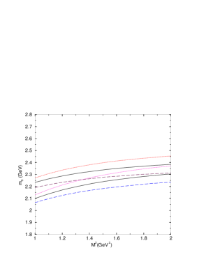
Figure 1: The $D_{0}^{(0s)}$ mass (the lower dashed, solid and dotted lines) and the $D_{0}^{(1s)}$ mass (the upper dashed, solid and dotted lines), as a function of the Borel mass for different values of the continuum threshold. Dashed lines: $\sqrt{s_{0}}=2.6\nobreak\,\mbox{GeV}$; solid lines: $\sqrt{s_{0}}=2.7\nobreak\,\mbox{GeV}$; dotted lines: $\sqrt{s_{0}}=2.8\nobreak\,\mbox{GeV}$.

We call $D_{0}^{(0s)}$, $D_{0}^{(1s)}$ and $D_{0}^{(2s)}$ the scalar charmed mesons represented by $j_{0}$, $j_{s}$ and $j_{ss}$ (in Eq. (1)) respectively. In Figs. 1 and 2 we show the masses of these three resonances as a function of the Borel mass for different values of the continuum threshold.

The Borel window was fixed in such way that the pole contribution is always between 80% and 20% of the total contribution.

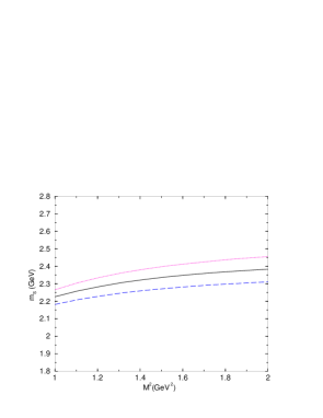
Figure 2: The $D_{0}^{(2s)}$ mass as a function of the Borel mass for different values of the continuum threshold. Dashed line: $\sqrt{s_{0}}=2.6\nobreak\,\mbox{GeV}$; solid line: $\sqrt{s_{0}}=2.7\nobreak\,\mbox{GeV}$; dotted line: $\sqrt{s_{0}}=2.8\nobreak\,\mbox{GeV}$.

Fixing $\sqrt{s_{0}}=2.7\nobreak\,\mbox{GeV}$ and varying the charm quark and the strange quark masses in the intervals: $1.1\leq m_{c}\leq 1.3\nobreak\,\mbox{GeV}$ and $0.11\leq m_{s}\leq 0.15\nobreak\,\mbox{GeV}$, we get results for the resonance masses still between the lower and upper lines in figures 1 and 2. A bigger value for the charm quark mass makes the results more stable as a function of the Borel mass. One can also vary the value of the quark condensate. Keeping the continuum threshold and the quark masses fixed at $\sqrt{s_{0}}=2.7\nobreak\,\mbox{GeV}$, $m_{c}=1.2\nobreak\,\mbox{GeV}$ and $m_{s}=0.13\nobreak\,\mbox{GeV}$ and varying the quark condensate in the interval: $\langle\bar{q}q\rangle=\,(-0.23\pm 0.01\nobreak\,\mbox{GeV})^{3}$, we get a bigger (smaller) result for the resonance masses using a smaller (bigger) value of the condensate. In Fig. 3 we show the the mass of the $D_{0}^{(1s)}$ state, as a function of the Borel mass, for the combination of the values of the continuum threshold and quark condensate that gives the lower and upper limits for the $D_{0}^{(1s)}$ mass.

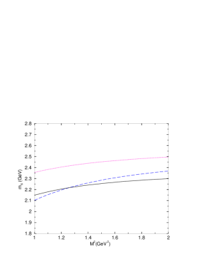
Figure 3: The $D_{0}^{(1s)}$ mass as a function of the Borel mass for different values of the continuum threshold and quark condensate. Solid line: $\sqrt{s_{0}}=2.6\nobreak\,\mbox{GeV}$ and $\langle\bar{q}q\rangle(1\nobreak\,\mbox{GeV})=\,(-0.24\nobreak\,\mbox{GeV})^{3}$; dotted line: $\sqrt{s_{0}}=2.8\nobreak\,\mbox{GeV}$ and $\langle\bar{q}q\rangle(1\nobreak\,\mbox{GeV})=\,(-0.22\nobreak\,\mbox{GeV})^{3}$; dashed line: $\sqrt{s_{0}}=2.6\nobreak\,\mbox{GeV}$, $\langle\bar{q}q\rangle(2\nobreak\,\mbox{GeV})=\,(-0.267\nobreak\,\mbox{GeV})^{3}$ and $m_{s}(2\nobreak\,\mbox{GeV})=0.10\nobreak\,\mbox{GeV}$.

In ref.jala it was shown that the renormalization scale was an important source of uncertainty, in the analysis of the $B$ meson decay constant. To check how the change of the scale would change our results we also show, through the dashed line in Fig. 3 , the result for the $D_{0}^{(1s)}$ resonance mass using the values of the strange quark mass and quark condensate at the scale $2\nobreak\,\mbox{GeV}$: $\langle\bar{q}q\rangle(2\nobreak\,\mbox{GeV})=\,(-0.267\nobreak\,\mbox{GeV})^{3}$ and $m_{s}(2\nobreak\,\mbox{GeV})=0.10\nobreak\,\mbox{GeV}$ jala . We see that we get a less stable result for the ressonance mass, but it is still compatible with the results at the scale $1\nobreak\,\mbox{GeV}$, considering the variation in the continuum threshold. Therefore, we conclude that it is the variation of the continuum threshold that causes the most significant variations in the resonance masses, and it is our most important source of uncertaintiy.

Comparing figures 1 and 2 we see that the $D_{0}^{(1s)}$ and $D_{0}^{(2s)}$ resonance masses are basicaly degenerated, while the mass of $D_{0}^{(0s)}$ is around $100\nobreak\,\mbox{MeV}$ smaller than the others. While it is natural to expect that the inclusion of a strange quark would increase the resonance mass by around the strange quark mass (as was the case when one goes from $D_{0}^{(0s)}$ to $D_{0}^{(1s)}$), it is really interesting to observe that this does not happen when one goes from $D_{0}^{(1s)}$ to $D_{0}^{(2s)}$. In terms of the OPE contributions, we can trace this behavior to the fact that the quark condensate term is smaller in $D_{0}^{(2s)}$ than in $D_{0}^{(1s)}$ (due to the change from $m_{c}\langle\bar{q}q\rangle$ to $m_{c}\langle\bar{s}s\rangle$), however the inclusion of the term proportional to $m_{s}m_{c}$ (which is not present in $D_{0}^{(1s)}$), compensates this decrease.

Considering the variations on the quark masses, the quark condensate and on the continuum threshold discussed above, in the Borel window considered here our results for the ressonance masses are given in Table I.

Table I: Numerical results for the resonance masses
resonance $D_{0}^{(0s)}$ $D_{0}^{(1s)}$ $D_{0}^{(2s)}$ mass (GeV) $~{}2.22\pm 0.21~{}$ $~{}2.32\pm 0.18~{}$ $~{}2.30\pm 0.20~{}$

Comparing the results in Table I with the resonance masses given by BABAR, BELLE and FOCUS: $D_{sJ}^{+}(2317)$, $D_{0}^{0}(2308)$ and $D_{0}^{0,+}(2405)$, we see that we can identify the four-quark states represented by $D_{0}^{(1s)}$ and $D_{0}^{(2s)}$ with the BABAR and BELLE resonances respectively. However, we do not find a four-quark state whose mass is compatible with the FOCUS resonances, $D_{0}^{0,+}(2405)$. Therefore, we associate the FOCUS resonances, $D_{0}^{0,+}(2405)$, with a scalar $c\bar{q}$ state, since its mass is completly in agreement with the predictions of the quark model in ref. god . It is also interesting to point out that a mass of about $2.4~{}\nobreak\,\mbox{GeV}$ is also compatible with the the QCD sum rule calculation for a $c\bar{q}$ scalar meson ht .

One can still argue that while a pole approximation is justified for the very narrow BABAR resonance, this may not be the case for the rather broad BELLE and FOCUS resonances. To check if the width of the resonances could modify the pattern observed in the masses of the four-quark states, we have modified the phenomenological side of the sum rule, in Eq. (5), through the introduction of a Breit-Wigner-type resonance form:

$$\Pi^{phen}(M^{2})=2f_{S}^{2}m_{S}^{8}\int_{(m_{\pi}+m_{D})^{2}}^{s_{0}}ds~{}e^{-s/M^{2}}\rho_{BW}(s)\;,$$ (20)

where

$$\rho_{BW}(s)={1\over\pi}{\Gamma(s)m_{S}\over(s-m_{S}^{2})^{2}+m_{S}^{2}\Gamma(s)^{2}},$$ (21)

with $\Gamma(s)=\Gamma_{0}{\sqrt{\lambda(s,m_{D}^{2},m_{\pi}^{2})\over\lambda(m_{S},m_{D}^{2},m_{\pi}^{2})}}{m_{S}^{2}\over s}$, and $\lambda(x,y,z)=x^{2}+y^{2}+z^{2}-2xy-2xz-2yz$.

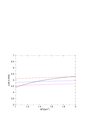
Figure 4: The RHS (solid line) and the LHS of the sum rule in Eq. (22) for $D_{0}^{(0s)}$, for different values of the resonance mass. Dashed line: $m_{S}=2.1\nobreak\,\mbox{GeV}$; dotted line: $m_{S}=2.2\nobreak\,\mbox{GeV}$; dot-dashed line: $m_{S}=2.3\nobreak\,\mbox{GeV}$.

Of course now we can not obtain an expression for the resonance mass as Eq. (19). However, we can still use the resonance mass as a parameter to compare the compatibility between the right-hand side (RHS) and the left-hand side (LHS) of the sum rule in Eq. (22):

$${\int_{(m_{\pi}+m_{D})^{2}}^{s_{0}}dse^{-s/M^{2}}s\rho_{BW}(s)\over\int_{(m_{\pi}+m_{D})^{2}}^{s_{0}}dse^{-s/M^{2}}\rho_{BW}(s)}={\int_{m_{c}^{2}}^{s_{0}}dse^{-s/M^{2}}s\rho_{S}(s)\over\int_{m_{c}^{2}}^{s_{0}}dse^{-s/M^{2}}\rho_{S}(s)}\;.$$ (22)

In Fig.4 we show the RHS (solid line) and the LHS of Eq. (22) for $D_{0}^{(0s)}$, for three different values of the resonance mass, with $\Gamma_{0}=280~{}\nobreak\,\mbox{MeV}$ and $\sqrt{s_{0}}=2.7~{}\nobreak\,\mbox{GeV}$. We see that the best agreement is obtained for $m_{S}\sim 2.2~{}\nobreak\,\mbox{GeV}$, which shows that the inclusion of the width does not change the value of the mass obtained for the resonance.

We have presented a QCD sum rule study of the charmed scalar mesons considered as diquark-antidiquark states. We found that the masses of the BABAR, $D_{sJ}^{+}(2317)$, and BELLE, $D_{0}^{0}(2308)$, resonances can be reproduced by the four-quark states $(cq)(\bar{q}\bar{s})$ and $(cs)(\bar{u}\bar{s})$ respectively. However, the mass of the FOCUS resonance, $D_{0}^{0,+}(2405)$, which we believe is not the same measured by BELLE, can not be reproduced in the four-quark state picture considered here. Therefore, we interpret it as a normal $c\bar{q}$ state, since its mass is in complete agreement with the predictions of the quark model in ref. god . We also obtain a mass of $\sim 2.2~{}\nobreak\,\mbox{GeV}$ for a four-quark scalar state $(cq)(\bar{u}\bar{d})$ which was not yet observed, and that should be also rather broad.

Acknowledgements: We would like to thank I. Bediaga for fruitful discussions. This work has been supported by CNPq and FAPESP.

References

(1) BABAR Coll., B. Auber et al., Phys. Rev. Lett.
90, 242001 (2003); Phys. Rev. D69, 031101 (2004).
(2) CLEO Coll., D. Besson et al., Phys. Rev. D68,
032002 (2003).
(3) BELLE Coll., P. Krokovny et al., Phys. Rev. Lett.
91, 262002 (2003).
(4) FOCUS Coll., E.W. Vaandering, hep-ex/0406044.
(5) S. Godfrey and N. Isgur, Phys. Rev. D32, 189 (1985);
S. Godfrey and R. Kokoshi, Phys. Rev. D43, 1679 (1991).
(6) BELLE Coll., K. Abe et al., Phys. Rev. D69,
112002 (2004).
(7) FOCUS Coll., J.M. Link et al., Phys. Lett.
B586, 11 (2004).
(8) Y.-B. Dai, C.-S. Huang, C. Liu and S.-L. Zhu,
Phys. Rev. D68, 114011 (2003).
(9) G.S. Bali, Phys. Rev. D68, 071501(R) (2003).
(10) A. Dougall, R.D. Kenway, C.M. Maynard and C. Mc-Neile,
Phys. Lett. B569, 41 (2003).
(11) A. Hayashigaki and K. Terasaki, hep-ph/0411285.
(12) S. Narison, Phys. Lett. B605, 319 (2005).
(13) T. Barnes, F.E. Close and H.J. Lipkin, Phys. Rev. D68,
054006 (2003).
(14) A.P. Szczepaniak, Phys. Lett. B567, 23 (2003).
(15) E. van Beveren and G. Rupp, Phys. Rev. Lett. 91,
012003 (2003).
(16) H.-Y. Cheng and W.-S. Hou, Phys. Lett. B566, 193 (2003).
(17) K. Terasaki, Phys. Rev. D68, 011501(R) (2003).
(18) L. Maiani, F. Piccinini, A.D. Polosa, V. Riquer,
Phys. Rev. D71, 014028 (2005).
(19) T. Browder, S. Pakvasa and A.A. Petrov, Phys. Lett.
B578, 365 (2004).