Reconstruction of the Neutrino Mixing Matrix and Leptonic Unitarity Triangles from Long-baseline Neutrino Oscillations

Abstract

We derive a new set of sum rules between the neutrino mass and mixing parameters in vacuum and their effective counterparts in matter. The moduli of nine genuine lepton mixing matrix elements can then be calculated in terms of the matter-corrected ones, and the latter can directly be determined from a variety of long-baseline neutrino oscillations. We show that it is possible to reconstruct the leptonic unitarity triangles and CP violation in a similar parametrization-independent way.

I Introduction

Thanks to the Super-Kamiokande [1] and SNO [2] experiments, both solar and atmospheric neutrino oscillations are convincingly established. It turns out that neutrinos do have masses and lepton flavors are really mixed, just as expected in some grand unified theories. Two neutrino mass-squared differences and three lepton mixing angles have been measured or constrained by current neutrino oscillation data [1, 2, 3, 4, 5]. A more precise determination of these parameters has to rely on the new generation of accelerator neutrino experiments with very long baselines [6], in which leptonic CP violation may also be observed. The terrestrial matter effects in all long-baseline neutrino experiments must be taken into account, since they can unavoidably modify the genuine behaviors of neutrino oscillations in vacuum.

To formulate the probabilities of neutrino oscillations in matter in the same form as those in vacuum, one may define the effective neutrino masses $\tilde{m}_{i}$ and the effective lepton flavor mixing matrix $\tilde{V}$ in which the terrestrial matter effects are already included. In this common approach, it is necessary to find out the relationship between the fundamental quantities of neutrino mixing in vacuum ($m_{i}$ and $V$) and their effective counterparts in matter ($\tilde{m}_{i}$ and $\tilde{V}$). The exact formulas of $\tilde{m}_{i}$ and $\tilde{V}$ as functions of $m_{i}$ and $V$ have been achieved by a number of authors [7, 8, 9, 10], and the similar expressions of $m_{i}$ and $V$ in terms of $\tilde{m}_{i}$ and $\tilde{V}$ have been derived in Ref. [11]. The latter case is equivalently interesting in phenomenology, because our physical purpose is to determine the fundamental parameters of lepton flavor mixing from the effective ones, whose values can directly be measured from a variety of long-baseline neutrino oscillation experiments.

This paper aims to reconstruct the genuine neutrino mixing matrix $V$ and its unitarity triangles from possible long-baseline neutrino oscillations with terrestrial matter effects. Our work is remarkably different from the existing ones [7, 8, 9, 10, 11] in the following aspects:

• We derive a new set of sum rules between $(m_{i},V)$ and $(\tilde{m}_{i},\tilde{V})$. It may perfectly complement the sum rules obtained in Ref. [12]. We show that similar results can be achieved in the four-neutrino mixing scheme.

• Our sum rules allow us to calculate the moduli of $V_{\alpha i}$ (for $\alpha=e,\mu,\tau$ and $i=1,2,3$) in terms of those of $\tilde{V}_{\alpha i}$. This approach, which results in some much simpler relations between $|V_{\alpha i}|^{2}$ and $|\tilde{V}_{\alpha i}|^{2}$, proves to be more useful than that proposed in our previous work [10]. The sides of three unitarity triangles can also be derived in a similar way.

• We express the neutrino oscillation probabilities in terms of $|\tilde{V}_{\alpha i}|^{2}$ and the matter-corrected Jarlskog parameter $\tilde{J}$ [13]. The fundamental lepton flavor mixing matrix $V$ and its unitarity triangles can then be reconstructed from possible long-baseline neutrino oscillations straightforwardly and parametrization-independently.

The only assumption to be made is a constant earth density profile. Such an assumption is rather reasonable and close to reality for most of the presently-proposed terrestrial long-baseline neutrino oscillation experiments [6], in which the neutrino beam is not expected to go through the earth’s core.

The remaining parts of this paper are organized as follows. In section II, we figure out a new set of sum rules between $(m_{i},V)$ and $(\tilde{m}_{i},\tilde{V})$ and discuss its extension in the four-neutrino mixing scheme. Section III is devoted to the calculation of $|V_{\alpha i}|^{2}$ in terms of $|\tilde{V}_{\alpha i}|^{2}$. We also show how to derive the sides of three unitarity triangles in a similar approach. In section IV, the neutrino oscillation probabilities are presented in terms of $|\tilde{V}_{\alpha i}|^{2}$ and $\tilde{J}$. We illustrate the dependence of different oscillation terms on the neutrino beam energy and the baseline length. Section V is devoted to a brief summary of our main results.

II New sum rules between $V$ and $\tilde{V}$

In the basis where the flavor eigenstates of charged leptons are identified with their mass eigenstates, the lepton flavor mixing matrix $V$ is defined to link the neutrino mass eigenstates ($\nu_{1},\nu_{2},\nu_{3}$) to the neutrino flavor eigenstates ($\nu_{e},\nu_{\mu},\nu_{\tau}$):

$$\left(\matrix{\nu_{e}\cr\nu_{\mu}\cr\nu_{\tau}\cr}\right)=\left(\matrix{V_{e1}&V_{e2}&V_{e3}\cr V_{\mu 1}&V_{\mu 2}&V_{\mu 3}\cr V_{\tau 1}&V_{\tau 2}&V_{\tau 3}\cr}\right)\left(\matrix{\nu_{1}\cr\nu_{2}\cr\nu_{3}\cr}\right)\;.$$ (1)

A similar definition can be made for $\tilde{V}$, the effective counterpart of $V$ in matter. The strength of CP violation in normal neutrino oscillations is measured by a rephasing-invariant quantity $J$ (in vacuum) or $\tilde{J}$ (in matter), the so-called Jarlskog parameter [13]:

$${\rm Im}\left(V_{\alpha i}V_{\beta j}V^{*}_{\alpha j}V^{*}_{\beta i}\right) = J\sum_{\gamma,k}\left(\epsilon^{~{}}_{\alpha\beta\gamma}\epsilon^{~{}}_{ijk}\right)\;,$$ (2)

$${\rm Im}\left(\tilde{V}_{\alpha i}\tilde{V}_{\beta j}\tilde{V}^{*}_{\alpha j}\tilde{V}^{*}_{\beta i}\right) = \tilde{J}\sum_{\gamma,k}\left(\epsilon^{~{}}_{\alpha\beta\gamma}\epsilon^{~{}}_{ijk}\right)\;,$$ (3)

where the Greek subscripts $(\alpha,\beta,\gamma)$ and the Latin subscripts $(i,j,k)$ run over $(e,\mu,\tau)$ and $(1,2,3)$, respectively.

The effective Hamiltonian responsible for the propagation of neutrinos in vacuum or in matter can be written as

$$H_{\nu} = \frac{1}{2E}(M_{\nu}M^{\dagger}_{\nu})=\frac{1}{2E}\left(VD^{2}_{\nu}V^{\dagger}\right)\;,$$ (4)

$$\tilde{H}_{\nu} = \frac{1}{2E}(\tilde{M}_{\nu}\tilde{M}^{\dagger}_{\nu})=\frac{1}{2E}\left(\tilde{V}\tilde{D}^{2}_{\nu}\tilde{V}^{\dagger}\right)\;,$$ (5)

where $D_{\nu}\equiv{\rm Diag}\{m^{2}_{1},m^{2}_{2},m^{2}_{3}\}$ and $\tilde{D}_{\nu}\equiv{\rm Diag}\{\tilde{m}^{2}_{1},\tilde{m}^{2}_{2},\tilde{m}^{2}_{3}\}$, $E$ is the neutrino beam energy, $M_{\nu}$ and $\tilde{M}_{\nu}$ denote the corresponding genuine and matter-corrected neutrino mass matrices in the chosen flavor basis, $m_{i}$ and $\tilde{m}_{i}$ (for $i=1,2,3$) stand respectively for the neutrino masses in vacuum and those in matter. The deviation of $\tilde{H}_{\nu}$ from $H_{\nu}$ results non-trivially from the charged-current contribution to the $\nu_{e}e^{-}$ forward scattering [14], when neutrinos travel through a normal material medium like the earth:

$$\tilde{H}_{\nu}-H_{\nu}\equiv\frac{1}{2E}\Omega_{\nu}={\rm Diag}\{a,0,0\}\;,~{}~{}$$ (6)

where $a=\sqrt{2}G_{\rm F}N_{e}$ with $N_{e}$ being the background density of electrons. Subsequently we assume a constant earth density profile (i.e., $N_{e}$ = constant), which is a very good approximation for most of the long-baseline neutrino experiments proposed at present.

Eq. (3) implies that $(M_{\nu}M^{\dagger}_{\nu})^{n}=VD^{2n}_{\nu}V^{\dagger}$ and $(\tilde{M}_{\nu}\tilde{M}^{\dagger}_{\nu})^{n}=\tilde{V}\tilde{D}^{2n}_{\nu}\tilde{V}^{\dagger}$ hold, in which $n=0,\pm 1,\pm 2$, etc. To be explicit, we obtain

$$(M_{\nu}M^{\dagger}_{\nu})^{n}_{\alpha\beta} = \sum^{3}_{i=1}\left(m^{2n}_{i}V_{\alpha i}V^{*}_{\beta i}\right)\;,$$ (7)

$$(\tilde{M}_{\nu}\tilde{M}^{\dagger}_{\nu})^{n}_{\alpha\beta} = \sum^{3}_{i=1}\left(\tilde{m}^{2n}_{i}\tilde{V}_{\alpha i}\tilde{V}^{*}_{\beta i}\right)\;,$$ (8)

where $\alpha$ and $\beta$ run over $e$, $\mu$ and $\tau$. The simplest connection between $(M_{\nu}M^{\dagger}_{\nu})^{n}$ and $(\tilde{M}_{\nu}\tilde{M}^{\dagger}_{\nu})^{n}$ is their linear relation with $n=1$; i.e.,

$$\tilde{M}_{\nu}\tilde{M}^{\dagger}_{\nu}=M_{\nu}M^{\dagger}_{\nu}+\Omega_{\nu}\;,$$ (9)

as indicated by Eqs. (3) and (4). With the help of Eqs. (5) and (6), one may easily find

$$\sum^{3}_{i=1}\left(\tilde{m}^{2}_{i}\tilde{V}_{\alpha i}\tilde{V}^{*}_{\beta i}\right)=\sum^{3}_{i=1}\left(m^{2}_{i}V_{\alpha i}V^{*}_{\beta i}\right)+A\delta_{\alpha e}\delta_{e\beta}\;,$$ (10)

where $A=2Ea$. In the $\alpha\neq\beta$ case, Eq. (7) reproduces the sum rules obtained in Ref. [12]. A new set of sum rules can be achieved, if the square relation

$$(\tilde{M}_{\nu}\tilde{M}^{\dagger}_{\nu})^{2}=(M_{\nu}M^{\dagger}_{\nu})^{2}+(M_{\nu}M^{\dagger}_{\nu})\Omega_{\nu}+\Omega_{\nu}(M_{\nu}M^{\dagger}_{\nu})+\Omega^{2}_{\nu}$$ (11)

is taken into account. Resolving Eq. (8) by use of Eqs. (4) and (5), we arrive at

$$\sum^{3}_{i=1}\left(\tilde{m}^{4}_{i}\tilde{V}_{\alpha i}\tilde{V}^{*}_{\beta i}\right)=\sum^{3}_{i=1}\left\{m^{2}_{i}\left[m^{2}_{i}+A\left(\delta_{\alpha e}+\delta_{e\beta}\right)\right]V_{\alpha i}V^{*}_{\beta i}\right\}+A^{2}\delta_{\alpha e}\delta_{e\beta}\;.$$ (12)

Eqs. (7) and (9), together with the unitarity conditions

$$\sum^{3}_{i=1}(\tilde{V}_{\alpha i}\tilde{V}^{*}_{\beta i})=\sum^{3}_{i=1}(V_{\alpha i}V^{*}_{\beta i})=\delta_{\alpha\beta}\;,$$ (13)

constitute a full set of linear equations of $V_{\alpha i}V^{*}_{\beta i}$ or $\tilde{V}_{\alpha i}\tilde{V}^{*}_{\beta i}$ for $i=1,2$ and 3. We shall make use of these equations to derive the concrete expressions of $V_{\alpha i}V^{*}_{\beta i}$ in terms of $m_{i}$, $\tilde{m}_{i}$ and $\tilde{V}_{\alpha i}\tilde{V}^{*}_{\beta i}$ in the next section.

It is worth remarking that the sum rules in Eq. (9) are completely different from those presented in Refs. [10, 15, 16, 17], where the relationship between $H^{-1}_{\nu}\det H_{\nu}$ and $\tilde{H}^{-1}_{\nu}\det\tilde{H}_{\nu}$ has been used. Our new result can appreciably simplify the calculations of $|V_{\alpha i}|^{2}$ in terms of $|\tilde{V}_{\alpha i}|^{2}$ (or vice versa), as one may see later.

Eqs. (7) and (9) may be generalized to include the mixing between one sterile neutrino ($\nu_{s}$) and three active neutrinos ($\nu_{e}$, $\nu_{\mu}$ and $\nu_{\tau}$). In this case, $V$ is redefined to link the neutrino mass eigenstates $(\nu_{0},\nu_{1},\nu_{2},\nu_{3})$ to the neutrino flavor eigenstates $(\nu_{s},\nu_{e},\nu_{\mu},\nu_{\tau})$:

$$\left(\matrix{\nu_{s}\cr\nu_{e}\cr\nu_{\mu}\cr\nu_{\tau}\cr}\right)=\left(\matrix{V_{s0}&V_{s1}&V_{s2}&V_{s3}\cr V_{e0}&V_{e1}&V_{e2}&V_{e3}\cr V_{\mu 0}&V_{\mu 1}&V_{\mu 2}&V_{\mu 3}\cr V_{\tau 0}&V_{\tau 1}&V_{\tau 2}&V_{\tau 3}\cr}\right)\left(\matrix{\nu_{0}\cr\nu_{1}\cr\nu_{2}\cr\nu_{3}\cr}\right)\;,$$ (14)

and $\tilde{V}$ can be redefined in the same manner. The matrices $D_{\nu}$, $\tilde{D}_{\nu}$ and $\Omega_{\nu}$ in Eqs. (3) and (4) are now rewritten as

$$D_{\nu} = {\rm Diag}\left\{m^{2}_{0},m^{2}_{1},m^{2}_{2},m^{2}_{3}\right\}\;,$$ (15)

$$\tilde{D}_{\nu} = {\rm Diag}\left\{\tilde{m}^{2}_{0},\tilde{m}^{2}_{1},\tilde{m}^{2}_{2},\tilde{m}^{2}_{3}\right\}\;,$$ (16)

$$\Omega_{\nu} = {\rm Diag}\left\{A^{\prime},A,0,0\right\}\;,$$ (17)

in which $m_{0}$ denotes the sterile neutrino’s mass, and $A^{\prime}=\sqrt{2}G_{\rm F}N_{n}E$ with $N_{n}$ being the background density of neutrons [18]. Different from $A$, $A^{\prime}$ measures the universal neutral-current interactions of $\nu_{e}$, $\nu_{\mu}$ and $\nu_{\tau}$ with terrestrial matter. Both $A$ and $A^{\prime}$ are assumed to be constant throughout this work. Then two sets of sum rules can respectively be derived from the linear and square relations given in Eqs. (6) and (8):

$$\sum^{3}_{i=0}\left(\tilde{m}^{2}_{i}\tilde{V}_{\alpha i}\tilde{V}^{*}_{\beta i}\right) = \sum^{3}_{i=0}\left(m^{2}_{i}V_{\alpha i}V^{*}_{\beta i}\right)+A^{\prime}\delta_{\alpha s}\delta_{s\beta}+A\delta_{\alpha e}\delta_{e\beta}\;,$$ (18)

$$\sum^{3}_{i=0}\left(\tilde{m}^{4}_{i}\tilde{V}_{\alpha i}\tilde{V}^{*}_{\beta i}\right) = \sum^{3}_{i=0}\left\{m^{2}_{i}\left[m^{2}_{i}+A^{\prime}\left(\delta_{\alpha s}+\delta_{s\beta}\right)+A\left(\delta_{\alpha e}+\delta_{e\beta}\right)\right]V_{\alpha i}V^{*}_{\beta i}\right\}$$ (20)

$$+{A^{\prime}}^{2}\delta_{\alpha s}\delta_{s\beta}+A^{2}\delta_{\alpha e}\delta_{e\beta}\;.$$

Of course, one may also make use of the relation between $(M_{\nu}M^{\dagger}_{\nu})^{3}$ and $(\tilde{M}_{\nu}\tilde{M}^{\dagger}_{\nu})^{3}$ to derive another set of sum rules between $(m_{i},V)$ and $(\tilde{m}_{i},\tilde{V})$, although the relevant calculations are somehow lengthy. It is then possible to establish a full set of linear equations of $\tilde{V}_{\alpha i}\tilde{V}^{*}_{\beta i}$ or $V_{\alpha i}V^{*}_{\beta i}$ for $i=0,1,2$ and 3 in the four-neutrino mixing scheme, from which both the moduli of $V_{\alpha i}$ and the sides of six unitarity quadrangles of $V$ [19] can be derived in terms of $A$, $A^{\prime}$ and the neutrino mass and mixing parameters in matter. Such an idea and its phenomenological consequences will be elaborated elsewhere.

III Moduli and unitarity triangles of $V$

Now let us calculate the moduli of $V_{\alpha i}$ by using Eqs. (7), (9) and (10) in the conventional three-neutrino mixing scheme, assuming that $|\tilde{V}_{\alpha i}|^{2}$ can directly be determined from possible long-baseline neutrino oscillation experiments. Those three equations are rewritten, in the $\alpha=\beta$ case, as follows:

$$O_{1}\left(\matrix{|V_{\alpha 1}|^{2}\cr|V_{\alpha 2}|^{2}\cr|V_{\alpha 3}|^{2}\cr}\right)=\tilde{O}_{1}\left(\matrix{|\tilde{V}_{\alpha 1}|^{2}\cr|\tilde{V}_{\alpha 2}|^{2}\cr|\tilde{V}_{\alpha 3}|^{2}\cr}\right)-\left(\matrix{0\cr A\cr A^{2}\cr}\right)\delta_{\alpha e}\;,$$ (21)

where

$$O_{1} = \left(\matrix{1&1&1\cr m_{1}^{2}&m_{2}^{2}&m_{3}^{2}\cr m_{1}^{2}\left(m_{1}^{2}+2A\delta_{\alpha e}\right)&m_{2}^{2}\left(m_{2}^{2}+2A\delta_{\alpha e}\right)&m_{3}^{2}\left(m_{3}^{2}+2A\delta_{\alpha e}\right)\cr}\right)\;,$$ (22)

$$\tilde{O}_{1} = \left(\matrix{1&1&1\cr\tilde{m}_{1}^{2}&\tilde{m}_{2}^{2}&\tilde{m}_{3}^{2}\cr\tilde{m}_{1}^{4}&\tilde{m}_{2}^{4}&\tilde{m}_{3}^{4}\cr}\right)\;.$$ (23)

With the help of the relationship [15]

$$\sum^{3}_{i=1}\tilde{m}^{2}_{i}=\sum^{3}_{i=1}m^{2}_{i}+A\;,$$ (24)

we solve Eq. (14) and obtain the following exact results:

$$|{V}_{e1}|^{2} = \frac{\widehat{\Delta}_{13}\widehat{\Delta}_{12}}{{\Delta}_{13}{\Delta}_{12}}|\tilde{V}_{e1}|^{2}+\frac{\widehat{\Delta}_{13}\widehat{\Delta}_{11}}{{\Delta}_{13}{\Delta}_{12}}|\tilde{V}_{e2}|^{2}+\frac{\widehat{\Delta}_{11}\widehat{\Delta}_{12}}{{\Delta}_{13}{\Delta}_{12}}|\tilde{V}_{e3}|^{2}\ ,$$ (25)

$$|{V}_{e2}|^{2} = \frac{\widehat{\Delta}_{22}\widehat{\Delta}_{23}}{{\Delta}_{21}{\Delta}_{23}}|\tilde{V}_{e1}|^{2}+\frac{\widehat{\Delta}_{21}\widehat{\Delta}_{23}}{{\Delta}_{21}{\Delta}_{23}}|\tilde{V}_{e2}|^{2}+\frac{\widehat{\Delta}_{21}\widehat{\Delta}_{22}}{{\Delta}_{21}{\Delta}_{23}}|\tilde{V}_{e3}|^{2}\ ,$$ (26)

$$|{V}_{e3}|^{2} = \frac{\widehat{\Delta}_{32}\widehat{\Delta}_{33}}{{\Delta}_{32}{\Delta}_{31}}|\tilde{V}_{e1}|^{2}+\frac{\widehat{\Delta}_{33}\widehat{\Delta}_{31}}{{\Delta}_{32}{\Delta}_{31}}|\tilde{V}_{e2}|^{2}+\frac{\widehat{\Delta}_{32}\widehat{\Delta}_{31}}{{\Delta}_{32}{\Delta}_{31}}|\tilde{V}_{e3}|^{2}\ ;$$ (27)

and

$$|{V}_{\mu 1}|^{2} = \frac{\widehat{\Delta}_{21}\widehat{\Delta}_{31}}{{\Delta}_{21}{\Delta}_{31}}|\tilde{V}_{\mu 1}|^{2}+\frac{\widehat{\Delta}_{22}\widehat{\Delta}_{32}}{{\Delta}_{21}{\Delta}_{31}}|\tilde{V}_{\mu 2}|^{2}+\frac{\widehat{\Delta}_{23}\widehat{\Delta}_{33}}{{\Delta}_{21}{\Delta}_{31}}|\tilde{V}_{\mu 3}|^{2}\ ,$$ (28)

$$|{V}_{\mu 2}|^{2} = \frac{\widehat{\Delta}_{11}\widehat{\Delta}_{31}}{{\Delta}_{12}{\Delta}_{32}}|\tilde{V}_{\mu 1}|^{2}+\frac{\widehat{\Delta}_{12}\widehat{\Delta}_{32}}{{\Delta}_{12}{\Delta}_{32}}|\tilde{V}_{\mu 2}|^{2}+\frac{\widehat{\Delta}_{13}\widehat{\Delta}_{33}}{{\Delta}_{12}{\Delta}_{32}}|\tilde{V}_{\mu 3}|^{2}\ ,$$ (29)

$$|{V}_{\mu 3}|^{2} = \frac{\widehat{\Delta}_{11}\widehat{\Delta}_{21}}{{\Delta}_{13}{\Delta}_{23}}|\tilde{V}_{\mu 1}|^{2}+\frac{\widehat{\Delta}_{12}\widehat{\Delta}_{22}}{{\Delta}_{13}{\Delta}_{23}}|\tilde{V}_{\mu 2}|^{2}+\frac{\widehat{\Delta}_{13}\widehat{\Delta}_{23}}{{\Delta}_{13}{\Delta}_{23}}|\tilde{V}_{\mu 3}|^{2}\ ;$$ (30)

and

$$|{V}_{\tau 1}|^{2} = \frac{\widehat{\Delta}_{21}\widehat{\Delta}_{31}}{{\Delta}_{21}{\Delta}_{31}}|\tilde{V}_{\tau 1}|^{2}+\frac{\widehat{\Delta}_{22}\widehat{\Delta}_{32}}{{\Delta}_{21}{\Delta}_{31}}|\tilde{V}_{\tau 2}|^{2}+\frac{\widehat{\Delta}_{23}\widehat{\Delta}_{33}}{{\Delta}_{21}{\Delta}_{31}}|\tilde{V}_{\tau 3}|^{2}\ ,$$ (31)

$$|{V}_{\tau 2}|^{2} = \frac{\widehat{\Delta}_{11}\widehat{\Delta}_{31}}{{\Delta}_{12}{\Delta}_{32}}|\tilde{V}_{\tau 1}|^{2}+\frac{\widehat{\Delta}_{12}\widehat{\Delta}_{23}}{{\Delta}_{12}{\Delta}_{23}}|\tilde{V}_{\tau 2}|^{2}+\frac{\widehat{\Delta}_{13}\widehat{\Delta}_{33}}{{\Delta}_{12}{\Delta}_{32}}|\tilde{V}_{\tau 3}|^{2}\ ,$$ (32)

$$|{V}_{\tau 3}|^{2} = \frac{\widehat{\Delta}_{11}\widehat{\Delta}_{21}}{{\Delta}_{13}{\Delta}_{23}}|\tilde{V}_{\tau 1}|^{2}+\frac{\widehat{\Delta}_{12}\widehat{\Delta}_{22}}{{\Delta}_{13}{\Delta}_{23}}|\tilde{V}_{\tau 2}|^{2}+\frac{\widehat{\Delta}_{13}\widehat{\Delta}_{23}}{{\Delta}_{13}{\Delta}_{23}}|\tilde{V}_{\tau 3}|^{2}\ ,$$ (33)

in which the neutrino mass-squared differences $\widehat{\Delta}_{ij}\equiv m^{2}_{i}-\tilde{m}^{2}_{j}$ and $\widetilde{\Delta}_{ij}\equiv\tilde{m}^{2}_{i}-\tilde{m}^{2}_{j}$ are defined. One can see that these results are more instructive and much simpler than those obtained in Ref. [10], because we have introduced a new set of sum rules in Eq. (9).

Next we calculate $V_{\alpha i}V^{*}_{\beta i}$ in terms of $\tilde{V}_{\alpha i}\tilde{V}^{*}_{\beta i}$ (for $\alpha\neq\beta$). The former can form three unitarity triangles in the complex plane, which were originally named as $\triangle_{e}$ with $(\alpha,\beta)=(\mu,\tau)$, $\triangle_{\mu}$ with $(\alpha,\beta)=(\tau,e)$, and $\triangle_{\tau}$ with $(\alpha,\beta)=(e,\mu)$ in Ref. [20]. Their effective counterparts in matter are then referred to as $\widetilde{\triangle}_{e}$, $\widetilde{\triangle}_{\mu}$ and $\widetilde{\triangle}_{\tau}$. Taking account of Eqs. (7), (9) and (10), one may easily write down a full set of equations of $V_{\alpha i}V^{*}_{\beta i}$ with $\alpha\neq\beta$:

$$O_{2}\left(\matrix{V_{\alpha 1}V^{*}_{\beta 1}\cr V_{\alpha 2}V^{*}_{\beta 2}\cr V_{\alpha 3}V^{*}_{\beta 3}\cr}\right)=\tilde{O}_{2}\left(\matrix{\tilde{V}_{\alpha 1}\tilde{V}^{*}_{\beta 1}\cr\tilde{V}_{\alpha 2}\tilde{V}^{*}_{\beta 2}\cr\tilde{V}_{\alpha 3}\tilde{V}^{*}_{\beta 3}\cr}\right)\;,$$ (34)

where

$$O_{2} = \left(\matrix{1&1&1\cr m_{1}^{2}&m_{2}^{2}&m_{3}^{2}\cr m_{1}^{2}\left[m_{1}^{2}+A\left(\delta_{\alpha e}+\delta_{e\beta}\right)\right]&m_{2}^{2}\left[m_{2}^{2}+A\left(\delta_{\alpha e}+\delta_{e\beta}\right)\right]&m_{3}^{2}\left[m_{3}^{2}+A\left(\delta_{\alpha e}+\delta_{e\beta}\right)\right]\cr}\right)\;,$$ (35)

$$\tilde{O}_{2} = \left(\matrix{1&1&1\cr\tilde{m}_{1}^{2}&\tilde{m}_{2}^{2}&\tilde{m}_{3}^{2}\cr\tilde{m}_{1}^{4}&\tilde{m}_{2}^{4}&\tilde{m}_{3}^{4}\cr}\right)\;.$$ (36)

We solve Eq. (20) and arrive at

$${V}_{\mu 1}{V}_{\tau 1}^{\ast} = \frac{(\widehat{\Delta}_{21}+\widehat{\Delta}_{33})\widetilde{\Delta}_{31}}{{\Delta}_{21}{\Delta}_{31}}\tilde{V}_{\mu 1}\tilde{V}_{\tau 1}^{\ast}+\frac{(\widehat{\Delta}_{22}+\widehat{\Delta}_{33})\widetilde{\Delta}_{32}}{{\Delta}_{21}{\Delta}_{31}}\tilde{V}_{\mu 2}\tilde{V}_{\tau 2}^{\ast}\ ,$$ (37)

$${V}_{\mu 2}{V}_{\tau 2}^{\ast} = \frac{(\widehat{\Delta}_{32}+\widehat{\Delta}_{11})\widetilde{\Delta}_{21}}{{\Delta}_{32}{\Delta}_{21}}\tilde{V}_{\mu 2}\tilde{V}_{\tau 2}^{\ast}+\frac{(\widehat{\Delta}_{11}+\widehat{\Delta}_{33})\widetilde{\Delta}_{31}}{{\Delta}_{32}{\Delta}_{21}}\tilde{V}_{\mu 3}\tilde{V}_{\tau 3}^{\ast}\ ,$$ (38)

$${V}_{\mu 3}{V}_{\tau 3}^{\ast} = \frac{(\widehat{\Delta}_{13}+\widehat{\Delta}_{22})\widetilde{\Delta}_{23}}{{\Delta}_{13}{\Delta}_{23}}\tilde{V}_{\mu 3}\tilde{V}_{\tau 3}^{\ast}+\frac{(\widehat{\Delta}_{11}+\widehat{\Delta}_{22})\widetilde{\Delta}_{21}}{{\Delta}_{13}{\Delta}_{23}}\tilde{V}_{\mu 1}\tilde{V}_{\tau 1}^{\ast}\$$ (39)

for $\triangle_{e}$; and

$${V}_{\tau 1}{V}_{e1}^{\ast} = \frac{\widehat{\Delta}_{12}\widetilde{\Delta}_{31}}{{\Delta}_{12}{\Delta}_{31}}\tilde{V}_{\tau 1}\tilde{V}_{e1}^{\ast}+\frac{\widehat{\Delta}_{11}\widetilde{\Delta}_{32}}{{\Delta}_{12}{\Delta}_{31}}\tilde{V}_{\tau 2}\tilde{V}_{e2}^{\ast}\ ,$$ (40)

$${V}_{\tau 2}{V}_{e2}^{\ast} = \frac{\widehat{\Delta}_{23}\widetilde{\Delta}_{21}}{{\Delta}_{23}{\Delta}_{21}}\tilde{V}_{\tau 2}\tilde{V}_{e2}^{\ast}+\frac{\widehat{\Delta}_{22}\widetilde{\Delta}_{31}}{{\Delta}_{23}{\Delta}_{21}}\tilde{V}_{\tau 3}\tilde{V}_{e3}^{\ast}\ ,$$ (41)

$${V}_{\tau 3}{V}_{e3}^{\ast} = \frac{\widehat{\Delta}_{31}\widetilde{\Delta}_{23}}{{\Delta}_{31}{\Delta}_{23}}\tilde{V}_{\tau 3}\tilde{V}_{e3}^{\ast}+\frac{\widehat{\Delta}_{33}\widetilde{\Delta}_{21}}{{\Delta}_{31}{\Delta}_{23}}\tilde{V}_{\tau 1}\tilde{V}_{e1}^{\ast}\$$ (42)

for $\triangle_{\mu}$; and

$${V}_{e1}{V}_{\mu 1}^{\ast} = \frac{\widehat{\Delta}_{12}\widetilde{\Delta}_{31}}{{\Delta}_{12}{\Delta}_{31}}\tilde{V}_{e1}\tilde{V}_{\mu 1}^{\ast}+\frac{\widehat{\Delta}_{11}\widetilde{\Delta}_{32}}{{\Delta}_{12}{\Delta}_{31}}\tilde{V}_{e2}\tilde{V}_{\mu 2}^{\ast}\ ,$$ (43)

$${V}_{e2}{V}_{\mu 2}^{\ast} = \frac{\widehat{\Delta}_{23}\widetilde{\Delta}_{21}}{{\Delta}_{23}{\Delta}_{21}}\tilde{V}_{e2}\tilde{V}_{\mu 2}^{\ast}+\frac{\widehat{\Delta}_{22}\widetilde{\Delta}_{31}}{{\Delta}_{23}{\Delta}_{21}}\tilde{V}_{e3}\tilde{V}_{\mu 3}^{\ast}\ ,$$ (44)

$${V}_{e3}{V}_{\mu 3}^{\ast} = \frac{\widehat{\Delta}_{31}\widetilde{\Delta}_{23}}{{\Delta}_{31}{\Delta}_{23}}\tilde{V}_{e3}\tilde{V}_{\mu 3}^{\ast}+\frac{\widehat{\Delta}_{33}\widetilde{\Delta}_{21}}{{\Delta}_{31}{\Delta}_{23}}\tilde{V}_{e1}\tilde{V}_{\mu 1}^{\ast}\$$ (45)

for $\triangle_{\tau}$, where $\Delta_{ij}\equiv m^{2}_{i}-m^{2}_{j}$ denote the neutrino mass-squared differences in vacuum. These results are exactly the same as those obtained in Ref. [10], although a different approach has been followed. Eq. (22), (23) or (24) allows us to establish a direct relation between $J$ and $\tilde{J}$ defined in Eq. (2). A straightforward calculation yields $\tilde{J}\widetilde{\Delta}_{21}\widetilde{\Delta}_{31}\widetilde{\Delta}_{32}=J\Delta_{21}\Delta_{31}\Delta_{32}$, which has been derived in Refs. [12, 21] in a different way.

For the sake of completeness, let us list the expressions of two independent ${\Delta}_{ij}$ in terms of their effective counterparts in matter.

$${\Delta}_{31} = \displaystyle\frac{1}{3}\sqrt{\tilde{x}^{2}-3\tilde{y}}\left[3\tilde{z}+\sqrt{3\left(1-\tilde{z}^{2}\right)}\right]\;,$$ (46)

$${\Delta}_{32} = \displaystyle\frac{1}{3}\sqrt{\tilde{x}^{2}-3\tilde{y}}\left[3\tilde{z}-\sqrt{3\left(1-\tilde{z}^{2}\right)}\right]\;,$$ (47)

where [11]

$$\tilde{x} = \widetilde{\Delta}_{21}+\widetilde{\Delta}_{31}-A\;,$$ (48)

$$\tilde{y} = \displaystyle\widetilde{\Delta}_{21}\widetilde{\Delta}_{31}-A\left[\widetilde{\Delta}_{21}\left(1-|\tilde{V}_{e2}|^{2}\right)+\widetilde{\Delta}_{31}\left(1-|\tilde{V}_{e3}|^{2}\right)\right]\;,$$ (49)

$$\tilde{z} = \displaystyle\cos\left[\frac{1}{3}\arccos\frac{2\tilde{x}^{3}-9\tilde{x}\tilde{y}-27A\widetilde{\Delta}_{21}\widetilde{\Delta}_{31}|\tilde{V}_{e1}|^{2}}{2\left(\tilde{x}^{2}-3\tilde{y}\right)^{3/2}}\right]\;.$$ (50)

Three independent $\widehat{\Delta}_{ij}$ can be expressed as

$$\widehat{\Delta}_{11} = \displaystyle\frac{1}{3}\tilde{x}-\frac{1}{3}\sqrt{\tilde{x}^{2}-3\tilde{y}}\left[\tilde{z}+\sqrt{3\left(1-\tilde{z}^{2}\right)}\right]\;,$$ (51)

$$\widehat{\Delta}_{22} = \displaystyle\frac{1}{3}\tilde{x}-\frac{1}{3}\sqrt{\tilde{x}^{2}-3\tilde{y}}\left[\tilde{z}-\sqrt{3\left(1-\tilde{z}^{2}\right)}\right]-\widetilde{\Delta}_{21}\;,$$ (52)

$$\widehat{\Delta}_{33} = \displaystyle\frac{1}{3}\tilde{x}+\frac{2}{3}\tilde{z}\sqrt{\tilde{x}^{2}-3\tilde{y}}~{}-\widetilde{\Delta}_{31}\;.$$ (53)

Note that $\widehat{\Delta}_{ij}=\Delta_{ij}+\widehat{\Delta}_{jj}=\widetilde{\Delta}_{ij}+\widehat{\Delta}_{ii}$ holds. Thus both ${\Delta}_{ij}$ and $\widehat{\Delta}_{ij}$ are fully calculable, once $\widetilde{\Delta}_{21}$, $\widetilde{\Delta}_{31}$, $A$, $|\tilde{V}_{e1}|$ and $|\tilde{V}_{e2}|$ (or $|\tilde{V}_{e3}|$) are specified.

Note that the afore-obtained results are only valid for neutrinos propagating in vacuum and interacting with matter. As for antineutrinos, the corresponding results can simply be obtained through the replacements $V\Longrightarrow V^{*}$ and $A\Longrightarrow-A$ (and $A^{\prime}\Longrightarrow-A^{\prime}$ for the four-neutrino mixing scheme).

IV Long-baseline neutrino oscillations

The matter-corrected moduli $|\tilde{V}_{\alpha i}|^{2}$ and the effective Jarlskog parameter $\tilde{J}$ can, at least in principle, be determined from a variety of long-baseline neutrino oscillation experiments. To be concrete, the survival probability of a neutrino $\nu_{\alpha}$ and its conversion probability into another neutrino $\nu^{~{}}_{\beta}$ are given by [15]

$$\tilde{P}(\nu_{\alpha}\rightarrow\nu_{\alpha}) = 1-4\sum\limits_{i<j}\left(|\tilde{V}_{\alpha i}\tilde{V}_{\alpha j}^{*}|^{2}\sin^{2}\tilde{F}_{ji}\right)\;,$$ (54)

$$\tilde{P}(\nu_{\alpha}\rightarrow\nu^{~{}}_{\beta}) = -4\sum\limits_{i<j}\left[{\rm Re}\left(\tilde{V}_{\alpha i}\tilde{V}_{\beta j}\tilde{V}_{\alpha j}^{*}\tilde{V}_{\beta i}^{*}\right)\sin^{2}\tilde{F}_{ji}\right]-8\tilde{J}\prod\limits_{i<j}\left(\sin\tilde{F}_{ji}\right)\ ,$$ (55)

where $(\alpha,\beta)$ run over $(e,\mu)$, $(\mu,\tau)$ or $(\tau,e)$, $\tilde{F}_{ji}\equiv 1.27\widetilde{\Delta}_{ji}L/E$ with $L$ being the baseline length (in unit of km) and $E$ being the neutrino beam energy (in unit of GeV), and $\tilde{J}$ has been defined in Eq. (2). The ${\rm Re}(\tilde{V}_{\alpha i}\tilde{V}_{\beta j}\tilde{V}_{\alpha j}^{*}\tilde{V}_{\beta i}^{*})$ term in $\tilde{P}(\nu_{\alpha}\rightarrow\nu^{~{}}_{\beta})$ can be expressed as

$${\rm Re}\left(\tilde{V}_{\alpha i}\tilde{V}_{\beta j}\tilde{V}_{\alpha j}^{*}\tilde{V}_{\beta i}^{*}\right)=\frac{1}{2}\left(|\tilde{V}_{\alpha k}\tilde{V}^{*}_{\beta k}|^{2}-|\tilde{V}_{\alpha i}\tilde{V}^{*}_{\beta i}|^{2}-|\tilde{V}_{\alpha j}\tilde{V}^{*}_{\beta j}|^{2}\right)\;$$ (56)

with $\alpha\neq\beta$ and $i\neq j\neq k$. Then we rewrite Eq. (28) as follows:

$$\tilde{P}(\nu_{\alpha}\rightarrow\nu_{\alpha}) = 1-4\left(|\tilde{V}_{\alpha 1}\tilde{V}_{\alpha 2}^{*}|^{2}\sin^{2}\tilde{F}_{21}+|\tilde{V}_{\alpha 1}\tilde{V}_{\alpha 3}^{*}|^{2}\sin^{2}\tilde{F}_{31}+|\tilde{V}_{\alpha 2}\tilde{V}_{\alpha 3}^{*}|^{2}\sin^{2}\tilde{F}_{32}\right)\;,$$ (57)

$$\tilde{P}(\nu_{\alpha}\rightarrow\nu^{~{}}_{\beta}) = -2\left[|\tilde{V}_{\alpha 1}\tilde{V}^{*}_{\beta 1}|^{2}S_{1}+|\tilde{V}_{\alpha 2}\tilde{V}^{*}_{\beta 2}|^{2}S_{2}+|\tilde{V}_{\alpha 3}\tilde{V}^{*}_{\beta 3}|^{2}S_{3}\right]-8\tilde{J}S^{~{}}_{J}\;,$$ (58)

where

$$S_{1} \equiv \sin^{2}\tilde{F}_{32}-\sin^{2}\tilde{F}_{21}-\sin^{2}\tilde{F}_{31}\;,$$ (59)

$$S_{2} \equiv \sin^{2}\tilde{F}_{31}-\sin^{2}\tilde{F}_{21}-\sin^{2}\tilde{F}_{32}\;,$$ (60)

$$S_{3} \equiv \sin^{2}\tilde{F}_{21}-\sin^{2}\tilde{F}_{31}-\sin^{2}\tilde{F}_{32}\;,$$ (61)

$$S^{~{}}_{J} \equiv \sin\tilde{F}_{21}\sin\tilde{F}_{31}\sin\tilde{F}_{32}\;.$$ (62)

Some comments on Eqs. (30) and (31) are in order.

• Three oscillation terms in $\tilde{P}(\nu_{\alpha}\rightarrow\nu_{\alpha})$ are associated with $|\tilde{V}_{\alpha i}\tilde{V}^{*}_{\alpha j}|^{2}$ (with $i\neq j$). Taking $i=1$ and $j=2$ for example, we obtain an effective unitarity triangle whose three sides are $\tilde{V}_{e1}\tilde{V}^{*}_{e2}$, $\tilde{V}_{\mu 1}\tilde{V}^{*}_{\mu 2}$ and $\tilde{V}_{\tau 1}\tilde{V}^{*}_{\tau 2}$ in the complex plane. This triangle was originally named as $\widetilde{\triangle}_{3}$ in Ref. [20]. Triangles $\widetilde{\triangle}_{1}$ (for $i=2$ and $j=3$) and $\widetilde{\triangle}_{2}$ (for $i=1$ and $j=3$) can similarly be defined. Their genuine counterparts in vacuum are referred to as $\triangle_{i}$ for $i=1,2$ and 3. If the sides of $\widetilde{\triangle}_{i}$ can all be determined from $\tilde{P}(\nu_{\alpha}\rightarrow\nu_{\alpha})$ in some disappearance neutrino oscillation experiments, it is then possible to calculate individual $|\tilde{V}_{\alpha i}|^{2}$ and to extract $|V_{\alpha i}|^{2}$ by using Eqs. (17), (18) and (19).

• Three sides of triangle $\widetilde{\triangle}_{e}$, $\widetilde{\triangle}_{\mu}$ or $\widetilde{\triangle}_{\tau}$ are associated with three oscillation terms $S_{i}$ (for $i=1,2,3$) of the appearance neutrino oscillation probability $\tilde{P}(\nu_{\alpha}\rightarrow\nu_{\beta})$, while the effective CP-violating parameter $\tilde{J}$ is relevant to the oscillation term $S_{J}$. To illustrate, we plot the dependence of $S_{i}$ and $S_{J}$ on the neutrino (or antineutrino) beam energy $E$ in Fig. 1, where two typical neutrino baselines $L=730~{}{\rm km}$ [6] and $L=2100~{}{\rm km}$ [22] have been taken. The input parameters include $\Delta_{21}\approx 8\times 10^{-5}~{}{\rm eV}^{2}$, $\Delta_{32}\approx 2.3\times 10^{-3}~{}{\rm eV}^{2}$, $\theta_{12}\approx 33^{\circ}$, $\theta_{23}\approx 45^{\circ}$, $\theta_{13}\approx 3^{\circ}$ and $\delta\approx 90^{\circ}$ in the standard parametrization of $V$ [15]. In addition, the terrestrial matter effects can approximately be described by $A\approx 2.28\times 10^{-4}{\rm eV}^{2}E/[{\rm GeV}]$ [23]. Fig. 1 shows that $S_{i}$ may have quite different behaviors, if the baseline length is sufficiently large (e.g., $L\sim 1000$ km or larger). Hence the proper changes of $E$ and (or) $L$ would allow us to determine the coefficients of $S_{i}$, i.e., $|\tilde{V}_{\alpha i}\tilde{V}^{*}_{\beta i}|^{2}$. The parameter $\tilde{J}$ can also be extracted from a suitable long-baseline neutrino oscillation experiment, because the dependence of $S_{J}$ on $E$ and $L$ is essentially different from that of $S_{i}$. Provided all or most of such measurements are realistically done, the moduli of $V_{\alpha i}$ and leptonic unitarity triangles $\triangle_{e}$, $\triangle_{\mu}$ and $\triangle_{\tau}$ may finally be reconstructed.

• It is clear that both types of neutrino oscillation experiments (i.e., appearance and disappearance) are needed, in order to get more information on lepton flavor mixing and CP violation. They are actually complementary to each other in determining the moduli of nine matrix elements of $V$ and its unitarity triangles. In practice, the full reconstruction of $V$ from $\tilde{V}$ requires highly precise and challenging measurements. A detailed analysis of the unitarity triangle reconstruction can be found from Ref. [24], in which the issues of experimental feasibility and difficulties have more or less been addressed.

Let us remark that the strategy of this paper is to establish the model-independent relations between $V$ and $\tilde{V}$, both their moduli and their unitarity triangles. Hence we have concentrated on the generic formalism instead of the specific scenarios or numerical analyses. Our exact analytical results are expected to be a very useful addition to the phenomenology of lepton flavor mixing and neutrino oscillations.

V Summary

We have derived a new set of sum rules between $(m_{i},V)$ and $(\tilde{m}_{i},\tilde{V})$ for both three- and four-neutrino mixing schemes. With the help of our sum rules, we have calculated the moduli of $V_{\alpha i}$ in terms of those of $\tilde{V}_{\alpha i}$. The sides of leptonic unitarity triangles $\triangle_{e}$, $\triangle_{\mu}$ and $\triangle_{\tau}$ can also be figured out in a similar way. We find that it is useful to express the neutrino oscillation probabilities in terms of $|\tilde{V}_{\alpha i}|^{2}$ and the matter-corrected Jarlskog parameter $\tilde{J}$. The fundamental lepton flavor mixing matrix $V$ and its six unitarity triangles can then be reconstructed, at least in principle, from a variety of long-baseline neutrino oscillations in a straightforward and parametrization-independent way.

Our analytically exact results will be applicable for the study of terrestrial long-baseline neutrino oscillations, from which much better understanding of the neutrino mass spectrum, lepton flavor mixing and CP violation can be achieved.

One of us (Z.Z.X.) is grateful to CSSM at the University of Adelaide, where this paper was written, for warm hospitality. Our work was supported in part by the National Nature Science Foundation of China.

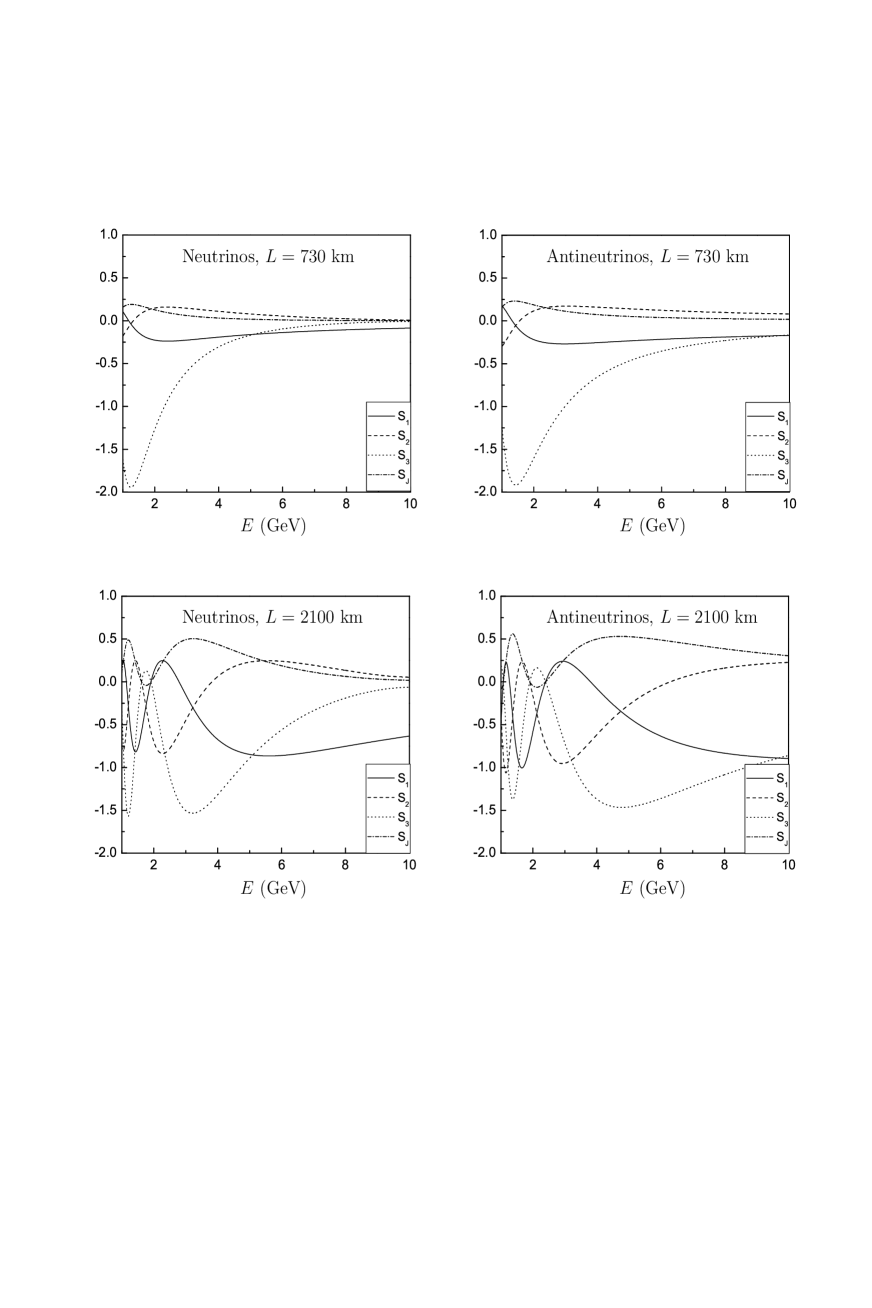
FIG. 1.: Numerical illustration of four different oscillation terms appearing in $\tilde{P}(\nu_{\alpha}\rightarrow\nu_{\beta})$ and $\tilde{P}(\overline{\nu}_{\alpha}\rightarrow\overline{\nu}_{\beta})$, where two typical neutrino beam baselines have been taken.