Global Analysis of Data on the Proton Structure Function $\mathbf{g}_{1}$
and Extraction of its Moments

Abstract

Inspired by recent measurements with the CLAS detector at Jefferson Lab, we perform a self-consistent analysis of world data on the proton structure function $g_{1}$ in the range $0.17<Q^{2}<30$ (GeV/c)². We compute for the first time low-order moments of $g_{1}$ and study their evolution from small to large values of $Q^{2}$. The analysis includes the latest data on both the unpolarized inclusive cross sections and the ratio $R=\sigma_{L}/\sigma_{T}$ from Jefferson Lab, as well as a new model for the transverse asymmetry $A_{2}$ in the resonance region. The contributions of both leading and higher twists are extracted, taking into account effects from radiative corrections beyond the next-to-leading order by means of soft-gluon resummation techniques. The leading twist is determined with remarkably good accuracy and is compared with the predictions obtained using various polarized parton distribution sets available in the literature. The contribution of higher twists to the $g_{1}$ moments is found to be significantly larger than in the case of the unpolarized structure function $F_{2}$.

I Introduction

One of the fundamental characterizations of nucleon structure is the distribution of the nucleon spin among its quark and gluon constituents. The classic tool for studying the quark spin distributions experimentally has been inclusive lepton scattering off polarized protons and neutrons. These experiments have determined the $g_{1}$ structure function of the nucleon, which, in the framework of the naïve Quark-Parton Model (QPM), is proportional to the difference between the distributions of quarks with spins aligned and anti-aligned to the nucleon spin. Surprisingly, one finds that only 20-30% of the proton spin is carried by quarks – an observation which came to be known as the “proton spin crisis”. Considerable effort, both experimentally and theoretically, has subsequently gone into understanding where the remaining fraction of the proton spin resides – see Ref. REVIEW for recent reviews.

In terms of kinematics, most of the experimental study has been focused on the high-$Q^{2}$ region, where the QPM description is most applicable, and in the region of intermediate and small Bjorken-$x$, which is important for evaluating parton model sum rules such as the Bjorken sum rule. Qualitatively new information on the proton spin structure can be obtained by studying the $g_{1}$ structure function in the region of large Bjorken-$x$, at moderate values of the squared four-momentum transfer $Q^{2}$, in the range from 1 to 5 (GeV/c)². Such a kinematic region is characterized by the presence of nucleon resonances which contribute to higher-twist effects in the structure functions.

According to the operator product expansion (OPE) in QCD, the $Q^{2}$-evolution of structure function moments can be described in terms of a $1/Q^{2}$, or twist, expansion, where the leading twist [${\cal{O}}(1)$ in $1/Q^{2}$] represents scattering from individual partons, while higher twists [${\cal{O}}(1/Q^{2})$ and higher] appear due to correlations among partons. The inclusion of the contribution from the nucleon resonance production regions is a relevant point of our study, because resonances and Deep Inelastic Scattering (DIS) are closely related by the phenomenon of local quark-hadron duality BloGil ; Rujula ; Ricco_dual . The latter has been extensively investigated at Jefferson Lab (JLab) for the case of the unpolarized structure function $F_{2}$ of the proton hallc ; f2mom-hc . In the polarized case, the contribution of the $\Delta(1232)$ resonance makes the analysis rather more interesting: since this resonance gives rise to a negative contribution to the $g_{1}$ structure function, while $g_{1}$ at high $Q^{2}$ is positive, one expects a breaking of local duality to occur in the $\Delta$ region at least up to several (GeV/c)² simula_g1 .

In this paper we report the results of a self-consistent extraction of the proton structure function $g_{1}(x,Q^{2})$ and its moments from the world data on the longitudinal polarization asymmetry $A_{\parallel}$. The extraction is based on a unique set of inputs for the structure function $F_{2}$, the ratio $R=\sigma_{L}/\sigma_{T}$ and the transverse asymmetry $A_{2}$. The complete data set measured at Jefferson Lab fatemi ; osipenko ; Hall-C-R , which covers the entire resonance region with high precision, allows for the first time the $Q^{2}$-evolution of the $g_{1}$ moments to be accurately evaluated up to $n=7$. The results for the first moment have been presented in Ref. M1p , where the twist-four matrix element was extracted, and the proton’s color electric and magnetic polarizabilities determined. Here we give the details of our analysis for all the moments up to $n=7$.

In Section II we describe the OPE framework of the moments analysis for the polarized structure function $g_{1}$. In Section III we discuss the extraction of $g_{1}$ from the longitudinal asymmetry $A_{\parallel}$. The evaluation of the moments of $g_{1}$ and their uncertainties is presented in Section III, and the extraction of both leading and higher twists is described in Section IV. Finally, conclusions from this study are summarized in Section V.

II Moments of the Structure Function $g_{1}$

The complete $Q^{2}$-evolution of the structure functions can be obtained using the OPE OPE of the time-ordered product of the two currents which enter into the virtual photon–nucleon forward Compton scattering amplitude,

$$T[J(z)~{}J(0)]=\sum_{n,\alpha}~{}f_{n}^{\alpha}(-z^{2})~{}z^{\mu_{1}}z^{\mu_{2}}...z^{\mu_{n}}~{}O_{\mu_{1}\mu_{2}...\mu_{n}}^{\alpha}$$ (1)

where $O_{\mu_{1}\mu_{2}...\mu_{n}}^{\alpha}$ are symmetric traceless operators of dimension $d_{n}^{\alpha}$ and twist $\kappa_{n}^{\alpha}\equiv d_{n}^{\alpha}-n$, with $\alpha$ labeling different operators of spin $n$. In Eq. (1), $f_{n}^{\alpha}(-z^{2})$ are coefficient functions, which are calculable in perturbative QCD (pQCD) at short light-cone distances $z^{2}=(ct)^{2}-\vec{z}^{2}\approx 0$. Since the imaginary part of the forward Compton scattering amplitude is simply the hadronic tensor containing the structure functions measured in DIS experiments, Eq. (1) leads to the well-known twist expansion for the Cornwall-Norton (CN) moments of $g_{1}(x,Q^{2})$ Corn-Nort ; Wandzura ,

$$M_{n}^{\rm CN}(Q^{2})\equiv\int_{0}^{1}dx~{}x^{n-1}~{}g_{1}^{N}(x,Q^{2})$$

$$=\sum_{\kappa=2,4~{}\cdots}^{\infty}E_{n\kappa}[\mu,\alpha_{s}(Q^{2})]~{}O_{n\kappa}(\mu)~{}\left({\mu^{2}\over Q^{2}}\right)^{(\kappa-2)/2}~{}~{}~{}~{}$$ (2)

for $n=1,3,5,\ldots$. Here $\mu$ is the renormalization scale, $O_{n\kappa}(\mu)$ are the (reduced) matrix elements of operators with definite spin $n$ and twist $\kappa$, containing information about the nonperturbative structure of the target, and $E_{n\kappa}(\mu,Q^{2})$ are dimensionless coefficient functions, which can be expressed perturbatively as a power series of the running coupling constant $\alpha_{s}(Q^{2})$.

In the Bjorken limit ($Q^{2},\nu\to\infty$, with $x=Q^{2}/2M\nu$ fixed, where $\nu$ is the energy transfer and $M$ the nucleon mass), only operators with spin $n$ contribute to the $n$-th CN moment (2). At finite $Q^{2}$, however, operators with different spins can contribute. Consequently the $1/Q^{2}$ expansion of the CN moment $M_{n}^{\rm CN}(Q^{2})$ contain in addition target-mass terms, proportional to powers of $M^{2}/Q^{2}$, which are formally leading twist and of pure kinematical origin. It was shown by Nachtmann Nachtmann in the unpolarized case, and subsequently generalized to the polarized structure functions in Ref. Wandzura , that even when $M^{2}/Q^{2}$ is nonzero, the moments can be redefined in such a way that only spin-$n$ operators contribute to the $n$-th moment. This is achieved by defining the “Nachtmann moments” of $g_{1}$ as

$$M_{n}(Q^{2}) \equiv \int_{0}^{1}dx{\xi^{n+1}\over x^{2}}$$ (3)

$$\times \left\{g_{1}(x,Q^{2})\left[{x\over\xi}-{n^{2}\over(n+2)^{2}}{M^{2}x^{2}\over Q^{2}}{\xi\over x}\right]\right.$$

$$-\left.g_{2}(x,Q^{2})~{}{M^{2}x^{2}\over Q^{2}}{4n\over n+2}\right\}~{}~{}~{}~{}$$

where $\xi=2x/\left(1+\sqrt{1+4M^{2}x^{2}/Q^{2}}\right)$ is the Nachtmann scaling variable. Note that the evaluation of the polarized moments $M_{n}(Q^{2})$ requires the knowledge of both structure functions $g_{1}$ and $g_{2}$. In the DIS regime the contribution of $g_{2}$ to Eq. (3) turns out to be typically small (see Ref. simula_g1 ). On the other hand, in the nucleon resonance production region the impact of $g_{2}$ is expected to be more significant, and here the lack of experimental information on the structure function $g_{2}$ can lead to systematic uncertainties.

Since the moments in Eq. (3) are totally inclusive, the integral in the right hand side of Eq. (3) contains also the contribution from the elastic peak located at $x=1$,

$$g_{1}^{\rm el}(x,Q^{2})=\delta(x-1)G_{M}(Q^{2})\frac{G_{E}(Q^{2})+\tau G_{M}(Q^{2})}{2(1+\tau)}$$ (4)

$$g_{2}^{\rm el}(x,Q^{2})=\delta(x-1)\tau G_{M}(Q^{2})\frac{G_{E}(Q^{2})-G_{M}(Q^{2})}{2(1+\tau)}~{}~{}~{}~{}$$ (5)

with $G_{E}$ $(G_{M})$ the proton electric (magnetic) elastic form factor and $\tau=Q^{2}/4M^{2}$.

Note that the structure function moments include the resonance production region at low $Q^{2}$ and high $x$, which would be otherwise problematic to include in a twist analysis performed directly in $x$-space. In addition, since target-mass corrections are by definition subtracted from the moments (3), the twist expansion of the Nachtmann moments $M_{n}(Q^{2})$ directly reveals information on the nonperturbative correlations between partons, without relying on specific assumptions about the $x$-shape of the leading twist.

For the leading twist contribution [$\kappa=2$ in Eq. (2)], one finds the well-known logarithmic $Q^{2}$ evolution of both singlet and non-singlet moments. However, if one wants to extend the analysis to small $Q^{2}$ and large $x$, where the rest of the perturbative series becomes significant, some procedure for the summation of higher orders of the pQCD expansion, such as infrared renormalon models renormalon ; Ricco1 or soft-gluon resummation techniques SGR ; SIM00 ; alpha , has to be applied. For higher twists, $\kappa>2$, the power-suppressed terms are related to quark-quark and quark-gluon correlations, as schematically illustrated in Fig. 1, and should become important at small $Q^{2}$.

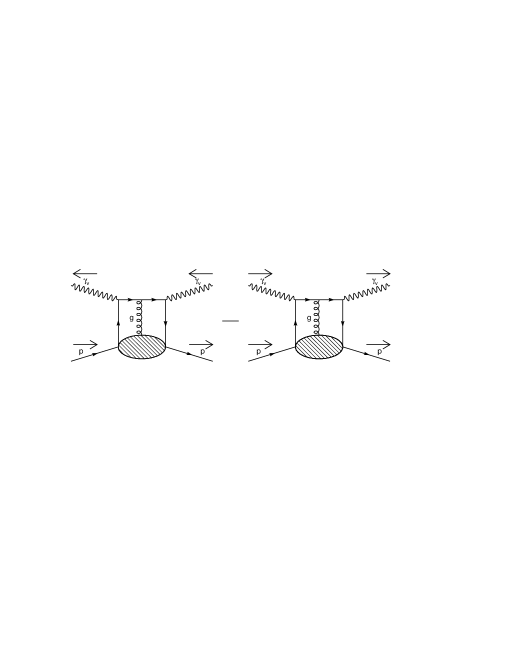
Figure 1: Example of a twist-4 diagram appearing in the OPE of polarized structure function moments. Arrows indicate the spin projections of the particles.

The evaluation of the Nachtmann moments (3) from available data in the range $0.17<Q^{2}<30$ (GeV/c)² will be described in the next section. The OPE analysis of such experimental moments will allow us to extract simultaneously both the leading and the higher twist contributions. A precise evaluation would permit a comparison of the leading twist with the QCD predictions obtained from lattice simulations or with nonperturbative models of the nucleon.

III Data Analysis

The data analysis was performed starting from measured longitudinal proton asymmetries $A_{\parallel}$, which were converted into the structure function $g_{1}$ using consistent values of the ratio $R=\sigma_{L}/\sigma_{T}$ and the structure function $F_{1}$, as well as of the transverse proton asymmetry $A_{2}$. Our procedure is described in detail in the following.

III.1 Asymmetry Database

All available world data on the longitudinal and transverse asymmetries, $A_{\parallel}$ and $A_{\perp}$, were collected from Refs. fatemi ; HERMES ; SLAC-E155x ; SLAC-E155 ; SLAC-E143 ; SLAC-E130 ; SLAC-E80 ; SMC-NA47 ; EMC-NA002 and Refs. HERMES ,SLAC-E155x ,SLAC-E155 b,SLAC-E80 b, respectively. The full data set of $A_{\parallel}$ consists of two subsets corresponding to the resonance fatemi and DIS regions HERMES ; SLAC-E155x ; SLAC-E155 ; SLAC-E143 ; SLAC-E130 ; SLAC-E80 ; SMC-NA47 ; EMC-NA002 . The kinematic coverage of the experimental data is shown in Figs. 2 and 3, for $A_{\parallel}$ and $A_{\perp}$, respectively. It can be seen that the resonance region is completely covered by the $A_{\parallel}$ data up to $Q^{2}=2.5$ (GeV/c)² with the inclusion of recent high quality data from CLAS fatemi .In contrast, the $A_{\perp}$ asymmetry is poorly determined in the resonance region. The lack of data on $A_{\perp}$ here becomes problematic because of the prominent role of the higher twist contributions at large values of $x$.

Figure 2: Kinematics of $A_{\parallel}$ world data from Refs. fatemi ; HERMES ; SLAC-E155x ; SLAC-E155 ; SLAC-E143 ; SLAC-E130 ; SLAC-E80 ; SMC-NA47 ; EMC-NA002 (different symbols indicate different experiments).

Figure 3: Kinematics of $A_{\perp}$ world data from Refs. HERMES ,SLAC-E155x ,SLAC-E155 b,SLAC-E80 b (different symbols indicate different experiments).

III.2 Extraction of the Structure Function $g_{1}$

In order to extract the structure function $g_{1}$ from the data collected in our data base, one needs additional experimental inputs for the structure function $F_{1}$, the ratio $R$, and the transverse asymmetry $A_{2}$. Indeed, the structure function $g_{1}$ is given by

$$g_{1}(x,Q^{2}) = \frac{F_{1}(x,Q^{2})}{1+\gamma^{2}}\Biggl{\{}\frac{A_{\parallel}(x,Q^{2})}{D}$$ (6)

$$+\ (\gamma-\eta)A_{2}(x,Q^{2})\Biggr{\}}\ ,$$

with

$$\gamma=\frac{2Mx}{\sqrt{Q^{2}}},~{}~{}\eta=\frac{\epsilon\sqrt{Q^{2}}}{E-\epsilon E^{\prime}},~{}~{}D=\frac{1-\epsilon E^{\prime}/E}{1+\epsilon R(x,Q^{2})}\ ,$$ (7)

where $E$ and $E^{\prime}$ are the incident and scattered electron energies and $\epsilon$ is the virtual photon polarization. The ratio $R$ entering above was taken from the parameterization given in Ref. Hall-C-R for the resonance production region, while in the DIS domain the fit R1998 r_fit_dis was used.

Since the main goal of our analysis is a model independent extraction of the moments of $g_{1}$, the structure function $F_{1}(x,Q^{2})$ has been obtained directly from experimental data. This has been possible because of the large amount of high quality data on the inclusive electron scattering cross section $d\sigma/d\Omega dE^{\prime}$ and on the structure function $F_{2}$, covering both the resonance and DIS regions (for the list of data used see Ref. osipenko ). Therefore, for each point of the measured longitudinal asymmetry $A_{\parallel}$ we can find several nearby points with either $F_{2}$ or the inclusive cross section known from experiments. For the interpolation of $F_{1}(x,Q^{2})$ points, a simple procedure has been used, which is described below.

Having a data point with the measured $A_{\parallel}$ at some fixed $x_{0}$ and $Q^{2}_{0}$, we search in the combined database on the inclusive cross section $d\sigma/d\Omega dE^{\prime}$ and the structure function $F_{2}$ for several nearby experimental points. The search procedure chooses a rectangular bin around the point with coordinates ($x_{0}$, $Q^{2}_{0}$) of such a size that the selected area contains a number $N$ of experimental points either from $d\sigma/d\Omega dE^{\prime}$ or from $F_{2}$. The procedure then selects only those configurations whose number of points $N_{min}<N<N_{max}$, where $N_{min}=2$ and $N_{max}=6$ in the resonance region and $N_{min}=1$ and $N_{max}=4$ in the DIS case. Once a number of configurations have been collected (no more than 20 sets), the procedure looks for a minimum in the sum of the path integrals from each point $(x_{i},Q^{2}_{i})$ of measured $d\sigma/d\Omega dE^{\prime}$ or $F_{2}$ to the bin center ($x_{0}$, $Q^{2}_{0}$),

$$S(x_{0},Q^{2}_{0})=\frac{1}{NF_{1}(x_{0},Q^{2}_{0})}\sum_{i}^{N}\int_{(x_{i},Q^{2}_{i})}^{(x_{0},Q^{2}_{0})}dl\ |F_{1}(x,Q^{2})|$$ (8)

where the integral over $dl$ is taken along a straight line connecting the point $(x_{i},Q^{2}_{i})$ to the bin center $(x_{0},Q^{2}_{0})$. The structure function $F_{1}(x,Q^{2})$ in this integral is constructed using the fits of $F_{2}$ from Ref. f2_fit_dis and of $R$ from Ref. r_fit_dis in DIS, while in the resonance production region $F_{1}$ is taken directly from Ref. Hall-C-R . The configuration selected is that which minimizes the function $S(x,Q^{2})$ in Eq. (8).

From Fig. 2, and also from Fig. 1 of Ref. osipenko , one can see that in the resonance region, which is covered by the data from Ref. fatemi , the interpolation distances are very small, thanks to the measurements of inclusive cross section in the same kinematic range osipenko ; hallc . A set of experimental points of $d\sigma/d\Omega dE^{\prime}$ or $F_{2}$ identified above is converted to the structure function $F_{1}$ according to

$$F_{1}(x,Q^{2})=\frac{MQ^{2}E}{2\alpha^{2}E^{\prime}}\frac{1-\epsilon}{1+\epsilon R(x,Q^{2})}\frac{d\sigma}{d\Omega dE^{\prime}}$$ (9)

and

$$F_{1}(x,Q^{2})=\frac{1+4M^{2}x^{2}/Q^{2}}{2x(1+R(x,Q^{2}))}F_{2}(x,Q^{2})~{}.$$ (10)

All the $F_{1}$ points obtained within the given bin are averaged together with their $x_{i}$ and $Q^{2}_{i}$ coordinates,

$$\overline{F_{1}}(x,Q^{2})=\frac{1}{\delta^{2}}\sum_{i}\frac{F_{1}(x_{i},Q^{2}_{i})}{\delta_{F_{1}}^{2}(x_{i},Q^{2}_{i})}~{},$$ (11)

$$\overline{x}=\frac{1}{\delta^{2}}\sum_{i}\frac{x_{i}}{\delta_{F_{1}}^{2}(x_{i},Q^{2}_{i})}~{},$$ (12)

$$\overline{Q^{2}}=\frac{1}{\delta^{2}}\sum_{i}\frac{Q^{2}_{i}}{\delta_{F_{1}}^{2}(x_{i},Q^{2}_{i})}~{},$$ (13)

where

$$\delta=\sqrt{\sum_{i}\frac{1}{\delta_{F_{1}}^{2}(x_{i},Q^{2}_{i})}}$$ (14)

and $\delta_{F_{1}}$ is the statistical error of $F_{1}$. The mean value of $\overline{F_{1}}(x,Q^{2})$ is then corrected by the bin centering correction using the models of Refs. f2_fit_dis ; r_fit_dis ; Hall-C-R . The value of the correction turns out to be very small with respect to statistical and systematic errors of the $A_{\parallel}$ data. Nevertheless, the correction value has been propagated in the total systematic error obtained for $\overline{F_{1}}$.

Once the transverse asymmetry $A_{\perp}$ is known, $A_{2}$ can be determined according to

$$A_{2}=\frac{1}{(1+\eta\zeta)}\Biggl{[}\frac{\zeta A_{\parallel}}{D}+\frac{A_{\perp}}{d}\Biggr{]}\ ,$$ (15)

where

$$d=D\sqrt{\frac{2\epsilon}{1+\epsilon}}\ ,~{}~{}~{}~{}~{}\zeta=\eta\frac{1+\epsilon}{2\epsilon}\ .$$ (16)

Since there are no experimental data on $A_{\perp}$ in the resonance region (see Fig. 3), we consider several models:

• The model-independent constraint provided by the Soffer limit Soffer :

  $$|A_{2}|<\sqrt{\frac{A_{1}+1}{2}R}~{}.$$ (17)

  This inequality is exact and, provided $A_{1}$ and $R(x,Q^{2})$ are measured, gives unambiguous limits.

• Since it was shown in previous experiments that $A_{2}$ is in fact much smaller than the Soffer limit SLAC-E155x , one can simply assume $A_{2}=0$, with possible deviations from zero included in the systematic error.

• In the present analysis we use a somewhat more sophisticated model for $A_{2}$ which is described in detail in Appendix A.

The $Q^{2}$ dependence of $g_{1}(x,Q^{2})$ at $x=0.38-0.42$ is shown in Fig. 4 using different assumptions about $A_{2}$ and $F_{1}$, which provides an estimate of the systematic errors. The ranges and the averages for the various sources of systematic errors on $g_{1}$ are collected in Table 1.

Figure 4: $Q^{2}$ dependence of the structure function $g_{1}$ at $x=0.38-0.42$ obtained from the data in Refs. fatemi ; HERMES ; SLAC-E155x ; SLAC-E155 ; SLAC-E143 ; SLAC-E130 ; SLAC-E80 ; SMC-NA47 ; EMC-NA002 using the procedure described in the text. Open squares represent central values obtained with the $A_{2}$ model described in Appendix A, while the filled triangles indicate upper and lower Soffer limits. The upper hatched area represents the difference between $g_{1}$ data points extracted with two different parameterizations of $R$ Hall-C-R ; Ricco1 ; middle hatched area $F_{1}^{MM}$ shows the difference between $g_{1}$ data points extracted using two different parameterizations of $F_{1}$ Hall-C-R ; Bodek ; lower hatched area $F_{1}^{DM}$ shows the difference between $g_{1}$ extracted from the $F_{1}$ parameterization and data interpolation as described in the text.

Table 1: Range and average of systematic errors on $g_{1}$ (absolute value).

Source of uncertainties	Variation range	Average
$A_{\parallel}$	10-4 – 0.14	0.015
$F_{1}$	10-7 – 1.7	0.014
$\sigma_{L}/\sigma_{T}$	10-4 – 0.015	0.002
$A_{2}$	10-7 – 0.015	0.004
Total	10-4 – 1.7	0.025

III.3 Moments of the Structure Function $g_{1}$

As discussed in the introduction, the final goal of our data analysis is the evaluation of the Nachtmann moments of the structure function $g_{1}$. The total Nachtmann moments were computed as the sum of the elastic ($M_{n}^{\rm el}$) and inelastic ($M_{n}^{\rm in}$) moments,

$$M_{n}(Q^{2})=M^{\rm el}_{n}(Q^{2})+M^{\rm in}_{n}(Q^{2})~{}.$$ (18)

The contribution from the elastic peak can be calculated by inserting Eqs. (4, 5) into Eq. (3),

$$M^{\rm el}_{n}(Q^{2}) = \frac{\xi^{n}_{\rm el}}{2}G_{M}(Q^{2})\Biggl{\{}\frac{G_{E}(Q^{2})+\tau G_{M}(Q^{2})}{1+\tau}$$ (19)

$$\times\Biggl{[}1-\frac{n^{2}}{(n+2)^{2}}\frac{M^{2}}{Q^{2}}\xi^{2}_{\rm el}\Biggl{]}$$

$$+ \frac{G_{M}(Q^{2})-G_{E}(Q^{2})}{1+\tau}\frac{n}{n+2}\xi_{\rm el}\Biggr{\}}~{},$$

where $\xi_{\rm el}=2/(1+\sqrt{1+1/\tau})$.

The evaluation of the inelastic moments $M^{\rm in}_{n}$ involves the computation at fixed $Q^{2}$ of an integral over $x$. In practice the integral over $x$ was performed numerically using the standard trapezoidal method in the program TRAPER cernlib .

The $Q^{2}$-range from 0.17 to 30 (GeV/c)² was divided into 24 bins increasing logarithmically with $Q^{2}$. Within each bin the world data were shifted to the central bin value $Q^{2}_{0}$ using the fit of $g_{1}^{S}(x,Q^{2})$ from Ref. simula_g1 , which covers both the resonance and DIS regions,

$$g_{1}(x,Q^{2}_{0})=g_{1}(x,Q^{2})+\left(g_{1}^{S}(x,Q^{2})-g_{1}^{S}(x,Q^{2}_{0})\right)~{}.$$ (20)

The difference between the actual and bin-centered data,

$$\delta^{cent}_{g_{1}}(x,Q^{2})=|g_{1}^{S}(x,Q^{2}_{0})-g_{1}^{S}(x,Q^{2})|~{},$$ (21)

is added to the systematic error of $g_{1}$ in the Nachtmann moments extraction procedure. As an example, Fig. 5 shows the integrands $I_{n}(x,Q^{2})$ of two of the low-order moments as a function of $x$ at fixed $Q^{2}$. The significance of the large-$x$ region for higher moments can be clearly seen.

Figure 5: Integrands of the Nachtmann moments at $Q^{2}=1$ GeV² for the $n=1$ (upper) and the $n=3$ (lower) moments.

To obtain a data set dense in $x$, which reduces the error in the numerical integration, we performed an interpolation at each fixed $Q^{2}_{0}$ when two contiguous experimental data points differed by more than $\nabla$. The value of $\nabla$ depends on kinematics: in the resonance regions, where the structure function exhibits strong variations, $\nabla$ has to be smaller than half of the resonance widths, and is parameterized as $\nabla=0.03~{}M^{2}/Q^{2}$. Above the resonances, where $g_{1}$ is smooth, to account for the fact that the available $x$ region decreases with decreasing $Q^{2}$, we set $\nabla=0.1$. Finally, in the low $x$ region ($x<0.03$) where the $g_{1}$ shape depends weakly on $Q^{2}$, but strongly on $x$, we set $\nabla=0.005$.

To fill the gap between two adjacent points $x_{a}$ and $x_{b}$, we used the interpolation function $g_{1}^{\rm int}(x,Q^{2}_{0})$, defined as the parameterization from Ref. simula_g1 offset to match the experimental data on both edges of the interpolating range. Assuming that the shape of the fit is correct, one has

$$g_{1}^{\rm int}(x,Q^{2}_{0})=\rho(Q^{2}_{0})+g_{1}^{S}(x,Q^{2}_{0})~{},$$ (22)

where the offset $\rho(Q^{2}_{0})$ is defined as the weighted average, evaluated using all experimental points located within an interval $\Delta$ around $x_{a}$ or $x_{b}$:

$$\rho(Q^{2}_{0}) = \delta_{N}^{2}(Q^{2}_{0})\Biggl{[}\sum\limits_{i}^{|x_{i}-x_{a}|<\Delta}\frac{g_{1}(x_{i},Q^{2}_{0})-g_{1}^{S}(x_{i},Q^{2}_{0})}{\bigl{(}\delta_{g_{1}}^{\rm stat}(x_{i},Q^{2}_{0})\bigr{)}^{2}}$$ (23)

$$+ \sum\limits_{j}^{|x_{j}-x_{b}|<\Delta}\frac{g_{1}(x_{j},Q^{2}_{0})-g_{1}^{S}(x_{j},Q^{2}_{0})}{\bigl{(}\delta_{g_{1}}^{\rm stat}(x_{j},Q^{2}_{0})\bigr{)}^{2}}\Biggr{]}~{},$$

where $\delta_{g_{1}}^{\rm stat}(x_{j},Q^{2}_{0})$ is the $g_{1}$ statistical error and

$$\delta_{N}(Q^{2}_{0}) = \Biggl{[}\sum\limits_{i}^{|x_{i}-x_{a}|<\Delta}\frac{1}{\bigl{(}\delta_{g_{1}}^{\rm stat}(x_{i},Q^{2}_{0})\bigr{)}^{2}}$$ (24)

$$+ \sum\limits_{j}^{|x_{j}-x_{b}|<\Delta}\frac{1}{\bigl{(}\delta_{g_{1}}^{\rm stat}(x_{j},Q^{2}_{0})\bigr{)}^{2}}\Biggr{]}^{-1/2}$$

is the statistical uncertainty of the normalization. Therefore, the statistical error of the moments calculated according to the trapezoidal rule cernlib was increased by adding the linearly correlated contribution from each interpolation interval as

$$\delta^{\rm norm}_{n}(Q^{2}_{0}) = \delta_{N}(Q^{2}_{0})\int\limits_{x_{a}}^{x_{b}}dx\frac{\xi^{n+1}}{x^{2}}g_{1}^{S}(x,Q^{2}_{0})$$ (25)

$$\times \Biggl{[}\frac{x}{\xi}-\frac{n^{2}}{(n+2)^{2}}\frac{M^{2}x^{2}}{Q^{2}_{0}}\frac{\xi}{x}\Biggr{]}~{}.$$

Since we average the difference $g_{1}(x_{i},Q^{2}_{0})-g_{1}^{S}(x_{i},Q^{2}_{0})$, $\Delta$ is not affected by the resonance structures, and its value is fixed to have more than two experimental points in most cases. Therefore, $\Delta$ is chosen to be equal to 0.15.

To fill the gap between the last experimental point and one of the integration limits ($x_{a}=0$ or $x_{b}=1$) we performed an extrapolation at each fixed $Q^{2}_{0}$ using $g_{1}^{S}(x,Q^{2}_{0})$ including its uncertainty given in Ref. simula_g1 . The results, together with their statistical and systematic errors, are presented in Table 2.

Table 2: The inelastic Nachtmann moments for $n=1,3,5$ and $7$ evaluated in the interval $0.17\leq Q^{2}\leq 30$ (GeV/c)². The moments were evaluated for $Q^{2}$ bins with more than 50% data coverage. The data are reported together with the statistical and systematic errors; the low-$x$ extrapolation error is given for the first moment only (last number in the second column).

$Q^{2}$ [(GeV/c)2]	$M_{1}(Q^{2})\times 10^{-3}$	$M_{3}(Q^{2})\times 10^{-4}$	$M_{5}(Q^{2})\times 10^{-5}$	$M_{7}(Q^{2})\times 10^{-6}$
0.17	–27.1 $\pm$ 7 $\pm$ 12 $\pm$ 6	–16.8 $\pm$ 2.5 $\pm$ 5	–8.5 $\pm$ 1 $\pm$ 2.5	–4.8 $\pm$ 0.6 $\pm$ 1.3
0.20	–23.0 $\pm$ 5 $\pm$ 9 $\pm$ 6	–17.0 $\pm$ 2 $\pm$ 4	–8.4 $\pm$ 0.8 $\pm$ 2	–4.3 $\pm$ 0.4 $\pm$ 1.1
0.24	–4.2 $\pm$ 4 $\pm$ 18 $\pm$ 7	–16.1 $\pm$ 2 $\pm$ 11	–11.0 $\pm$ 1 $\pm$ 7	–7.3 $\pm$ 0.7 $\pm$ 4.5
0.30	–8.9 $\pm$ 4 $\pm$ 19 $\pm$ 4	–26.6 $\pm$ 2 $\pm$ 14	–22.8 $\pm$ 1.5 $\pm$ 11	–18.8 $\pm$ 1.2 $\pm$ 9.3
0.35	9.6 $\pm$ 3 $\pm$ 12 $\pm$ 6	–23.9 $\pm$ 2 $\pm$ 8	–28.9 $\pm$ 2 $\pm$ 7.5	–31.2 $\pm$ 1.5 $\pm$ 7.4
0.42	28.0 $\pm$ 5 $\pm$ 11 $\pm$ 7	–13.9 $\pm$ 4 $\pm$ 9	–26.6 $\pm$ 4 $\pm$ 10	–37.9 $\pm$ 5 $\pm$ 12
0.50	36.3 $\pm$ 4 $\pm$ 17 $\pm$ 3	–13.2 $\pm$ 4 $\pm$ 16	–31.0 $\pm$ 5 $\pm$ 20	–48.4 $\pm$ 6 $\pm$ 27
0.60	43.4 $\pm$ 3.5 $\pm$ 15 $\pm$ 4	–12.2 $\pm$ 3 $\pm$ 16	–35.9 $\pm$ 4 $\pm$ 24	–64.5 $\pm$ 7 $\pm$ 38
0.70	56.0 $\pm$ 3 $\pm$ 14 $\pm$ 6	–0.1 $\pm$ 3 $\pm$ 18	–28.4 $\pm$ 4 $\pm$ 30	–71.7 $\pm$ 7 $\pm$ 53
0.84	69.0 $\pm$ 3 $\pm$ 13 $\pm$ 1.5	15.3 $\pm$ 3 $\pm$ 19	–8.7 $\pm$ 5 $\pm$ 36	–48.4 $\pm$ 11 $\pm$ 74
1.00	85.3 $\pm$ 3 $\pm$ 11 $\pm$ 0.7	25.7 $\pm$ 2.5 $\pm$ 17	–7.0 $\pm$ 5 $\pm$ 37	–81.1 $\pm$ 11 $\pm$ 84
1.20	94.2 $\pm$ 3.5 $\pm$ 10 $\pm$ 1	53.7 $\pm$ 3 $\pm$ 17	57 $\pm$ 7 $\pm$ 39	62.5 $\pm$ 18 $\pm$ 101
1.40	102 $\pm$ 4 $\pm$ 11 $\pm$ 2	68.6 $\pm$ 4 $\pm$ 20	88 $\pm$ 7 $\pm$ 48	123 $\pm$ 19 $\pm$ 133
1.70	114 $\pm$ 3 $\pm$ 16 $\pm$ 2	92.9 $\pm$ 5 $\pm$ 20	150 $\pm$ 11 $\pm$ 48	295 $\pm$ 32 $\pm$ 142
2.40	120 $\pm$ 2.5 $\pm$ 9 $\pm$ 3	108 $\pm$ 4 $\pm$ 16	218 $\pm$ 14 $\pm$ 46	572 $\pm$ 53 $\pm$ 152
3.00	124 $\pm$ 3 $\pm$ 8 $\pm$ 3	107 $\pm$ 4 $\pm$ 10
3.50	113 $\pm$ 7 $\pm$ 18 $\pm$ 1
4.20	125 $\pm$ 4 $\pm$ 9 $\pm$ 3.5	110 $\pm$ 4.5 $\pm$ 7
5.00	118 $\pm$ 5 $\pm$ 11 $\pm$ 4	85.3 $\pm$ 7 $\pm$ 16	153 $\pm$ 18 $\pm$ 59	398 $\pm$ 61 $\pm$ 236
6.00	122 $\pm$ 5.5 $\pm$ 8 $\pm$ 2	102 $\pm$ 6 $\pm$ 8	219 $\pm$ 17 $\pm$ 18	664 $\pm$ 84 $\pm$ 56
8.40		102 $\pm$ 4 $\pm$ 7
10.00	128 $\pm$ 11 $\pm$ 13 $\pm$ 4			565 $\pm$ 85 $\pm$ 66
15.50	130 $\pm$ 3 $\pm$ 16 $\pm$ 4	88.8 $\pm$ 3 $\pm$ 16	187 $\pm$ 10 $\pm$ 30	597 $\pm$ 51 $\pm$ 80
30.00	125 $\pm$ 4 $\pm$ 10 $\pm$ 2.5	78.7 $\pm$ 5 $\pm$ 11	158 $\pm$ 20 $\pm$ 23

III.4 Systematic Errors of the Moments

The systematic error consists of experimental uncertainties in the data given in Refs. fatemi ; HERMES ; SLAC-E155x ; SLAC-E155 ; SLAC-E143 ; SLAC-E130 ; SLAC-E80 ; SMC-NA47 ; EMC-NA002 and uncertainties in the evaluation procedure. To estimate the first type of error we have to account for using many data sets measured at different laboratories and with different detectors. In the present analysis we assume that different experiments are independent and therefore only systematic errors within a particulardata set are correlated.

An upper limit for the contribution of the systematic error from each data set was thus evaluated as follows:

• we first applied a simultaneous shift to all experimental points in the data set by an amount equal to their systematic error;

• the inelastic $n$-th moment obtained using these distorted data $\widetilde{M}^{\rm in}_{n(i)}(Q^{2})$ is then compared to the original moments $M^{\rm in}_{n}(Q^{2})$ evaluated with no systematic shifts;

• finally, the deviations for each data set were summed in quadrature as independent values,

  $$\delta_{n}^{D}(Q^{2})=\sqrt{\sum\limits_{i}^{N_{S}}\Bigl{(}\widetilde{M}^{\rm in}_{n(i)}(Q^{2})-M^{\rm in}_{n}(Q^{2})\Bigr{)}^{2}}~{},$$ (26)

  where $N_{S}$ is the number of available data sets. The resulting error is summed in quadrature with $\delta_{n}^{\rm norm}(Q^{2})$ to get the total systematic error on the $n$-th moment.

The second type of error is related to the bin centering, interpolation and extrapolation. The bin centering systematic uncertainty was estimated as

$$\delta^{C}_{n}(Q^{2})=\sum_{i}K_{n}(x_{i},Q^{2})w_{i}(Q^{2})\delta^{cent}_{g_{1}}(x_{i},Q^{2})~{},$$ (27)

where, according to the Nachtmann moment definition and the trapezoidal integration rule, one has

$$K_{n}(x_{i},Q^{2}) = \frac{\xi_{i}^{n+1}}{x_{i}^{2}}g_{1}(x,Q^{2})\Biggl{[}\frac{x_{i}}{\xi_{i}}-\frac{n^{2}}{(n+2)^{2}}\frac{M^{2}x_{i}^{2}}{Q^{2}}\frac{\xi_{i}}{x_{i}}\Biggr{]}\ ,$$

$$w_{i}(Q^{2}) = (x_{i+1}-x_{i-1})/2~{}.$$ (28)

The systematic error of the interpolation was estimated by considering the possible change of the fitting function slope in the interpolation interval, and was evaluated as a difference in the normalization at different edges:

$$\delta_{S}(Q^{2}_{0}) = \Biggl{|}\frac{1}{N_{i}}\sum\limits_{i}^{|x_{i}-x_{a}|<\Delta}(g_{1}(x_{i},Q^{2}_{0})-g_{1}^{S}(x_{i},Q^{2}_{0}))$$ (29)

$$- \frac{1}{N_{j}}\sum\limits_{j}^{|x_{j}-x_{b}|<\Delta}(g_{1}(x_{j},Q^{2}_{0})-g_{1}^{S}(x_{j},Q^{2}_{0}))\Biggr{|},~{}~{}~{}~{}$$

where $N_{i}$ and $N_{j}$ are the number of points used to evaluate the sums. Since the structure function $g_{1}(x,Q^{2})$ is a smooth function of $x$ below resonances, on the limited $x$-interval (smaller than $\nabla$) the linear approximation gives a good estimate. Thus, the error given in Eq. (29) accounts for such a linear mismatch between the fitting function and the data on the interpolation interval. Meanwhile, the CLAS data cover all the resonance region and no interpolation was used there. The total systematic error introduced in the corresponding moment by the interpolation can therefore be estimated as

$$\delta^{I}_{n}(Q^{2}_{0}) = \delta_{S}(Q^{2}_{0})\int\limits_{x_{a}}^{x_{b}}dx\frac{\xi^{n+1}}{x^{2}}g_{1}^{S}(x,Q^{2})$$ (30)

$$\times \Biggl{[}\frac{x}{\xi}-\frac{n^{2}}{(n+2)^{2}}\frac{M^{2}x^{2}}{Q^{2}}\frac{\xi}{x}\Biggr{]}~{}.$$

The systematic errors obtained by these procedures are then summed in quadrature to give,

$$\delta^{P}_{n}(Q^{2})=\sqrt{(\delta^{D}_{n}(Q^{2}))^{2}+(\delta^{C}_{n}(Q^{2}))^{2}+(\delta^{I}_{n}(Q^{2}))^{2}}~{}.$$ (31)

In order to study the systematic error on the extrapolation at very low $x$ we compared the moments extracted using different parameterizations of $g_{1}$. We choose a Regge inspired form from Ref. simula_g1 and two QCD fits from Refs. GRSV ; DS . The difference was significant only for $M_{1}$, for which the various errors are shown in Fig. 6 and separately given in Table 2.

Figure 6: Errors of the inelastic Nachtmann moment $M_{1}$: the empty circles represent statistical errors; the stars show the systematic error obtained in Eq. (31); the low-x extrapolation error is indicated by filled squares.

According to Eq. (18) the contribution from the proton elastic peak should be added to the inelastic moments obtained above. The $Q^{2}$-dependence of the proton elastic form factors is parameterized as in Ref. Bosted , modified accordingly to the recent data on $G_{E}/G_{M}$ hall-a , as described in Ref. CLAS_note . The uncertainty on the form factors is taken to be equal to 3% according to the analysis of Ref. Bosted , and is added quadratically to both the statistic and the systematic errors. The elastic contribution $M_{n}^{\rm el}(Q^{2})$ turns out to be a quite small correction for $Q^{2}\gtrsim n~{}({\rm GeV/c})^{2}$. Our final results for the total (inelastic + elastic) moments with $n=1,3,5$ and $7$ are shown in Fig. 7. Note also that the amount of the measured experimental contribution to $M_{n}(Q^{2})$ is at least 50%, and the systematic uncertainties increase significantly as $Q^{2}$ increases.

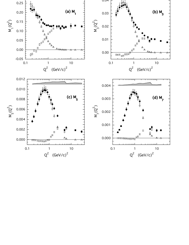
Figure 7: Total (inelastic + elastic) Nachtmann moments $M_{n}(Q^{2})$ (filled circles) [see Eq. (18)] extracted from the proton world data in the range $0.17\leq Q^{2}\leq 30$ (GeV/c)² for $n=1,3,5$ and $7$. Open squares and triangles correspond to the inelastic and elastic contributions, respectively. Statistical errors are reported for all the three terms; in case of the total moments the systematic errors are represented by the shaded bands.

IV Extraction of leading and higher twists

In this section we present our analysis of the moments $M_{n}(Q^{2})$ with $n>1$. We extract both the leading and higher twist contributions to the moments, including a determination of the effective anomalous dimensions.

Results for the first moment $M_{1}(Q^{2})$ were presented in Ref. M1p . There the highest $Q^{2}$-points [$Q^{2}>5~{}({\rm GeV/c})^{2}$] were used to obtain the singlet axial charge, which for the renormalization group invariant definition in the $\overline{{\rm MS}}$ scheme (which is adopted throughout this paper) gave: $a_{0}^{\rm inv}=0.145\pm 0.018(\mbox{{\rm stat.}})\pm 0.103(\mbox{{\rm sys.}})\pm 0.041({\rm low}x)\pm_{0.010}^{0.006}(\alpha_{s})$, where the first and second errors are statistical and systematic, the third is from the $x\to 0$ extrapolation, and the last is due to the uncertainty in $\alpha_{s}$. From the $Q^{2}$-dependence of the first moment the matrix elements of twist-4 operators were extracted, which allowed a precise determination of the color electric and magnetic polarizabilities of the proton (see Ref. M1p for details).

As has been discussed in Refs. Ricco1 ; SIM00 ; simula_g1 ; osipenko , the extraction of higher twists at large $x$ is sensitive to the effects of high-order pQCD corrections, for both the polarized and unpolarized cases. In particular, the use of the next-to-leading order (NLO) approximation for the leading twist is known to lead to unreliable results for the determination of the higher twists in the proton $F_{2}$ at large $x$ SIM00 . In this work we follow Refs. SIM00 ; simula_g1 ; osipenko , where the pQCD corrections beyond the NLO are estimated according to soft gluon resummation (SGR) techniques SGR and a pure non-singlet (NS) evolution is assumed for $n\geq 3$ . However, in contrast to Refs. SIM00 ; simula_g1 ; osipenko , where SGR was considered for the quark coefficient function only, we consistently add in this work the resummation of large-$n$ logarithms appearing also in the one-loop and two-loop NS anomalous dimensions. This was previously used in Ref. alpha to determine the strong coupling constant $\alpha_{s}(M_{Z}^{2})$ from the experimental moments of the proton $F_{2}$ structure function determined in Ref. osipenko .

Within the above framework, the Nachtmann moment of the leading twist part of the $g_{1}$ structure function, $\delta\eta_{n}(Q^{2})$, is (for $n\geq 3$) explicitly given by

$$\delta\eta_{n}(Q^{2}) = \delta A_{n}\left[\alpha_{s}(Q^{2})\right]^{\gamma_{n}^{{\rm NS}}}\left\{{\alpha_{s}(Q^{2})\over 4\pi}\delta R_{n}^{\rm NS}+e^{G_{n}(Q^{2})}\right.$$ (32)

$$\times \left.\left[1+{\alpha_{s}(Q^{2})\over 4\pi}\left(2C_{\rm DIS}^{({\rm NLO})}+\Delta\gamma_{\rm DIS}^{(1,{\rm NS})}\right)\right]\right\}~{}~{}~{}~{}$$

where the constant $\delta A_{n}$ is defined to be the $n$-th moment of the leading twist at the renormalization scale $\mu^{2}$, and $\gamma_{n}^{\rm NS}$ is the one-loop NS anomalous dimension. In Eq. (32) the quantity $\delta R_{n}^{\rm NS}$ is given by

$$\delta R_{n}^{\rm NS} = 2\left[\delta C_{n}^{({\rm NLO})}-C_{{\rm DIS}}^{({\rm NLO})}-C_{n,{\rm LOG}}^{({\rm NLO})}\right]$$ (33)

$$+ \Delta\gamma_{n}^{(1,{\rm NS})}-\Delta\gamma_{{\rm DIS}}^{(1,{\rm NS})}-\Delta\gamma_{n,{\rm LOG}}^{(1,{\rm NS})}$$

where

$$\Delta\gamma_{n}^{(1,{\rm NS})}\equiv\gamma_{n}^{(1,{\rm NS})}-{\beta_{1}\over\beta_{0}}\gamma_{n}^{\rm NS}$$ (34)

with $\gamma_{n}^{(1,{\rm NS})}$ being the two-loop NS anomalous dimension, $\beta_{0}=11-2N_{f}/3$, $\beta_{1}=102-38N_{f}/3$ and $N_{f}$ the number of active quark flavors at the scale $Q^{2}$.

In Eq. (33) $\delta C_{n}^{({\rm NLO})}$ is the NLO part of the quark coefficient function, which in the $\overline{{\rm MS}}$ scheme is given by

$$\delta C_{n}^{({\rm NLO})} = C_{F}\left\{S_{1}(n)\left[S_{1}(n)+{3\over 2}-{1\over n(n+1)}\right]\right.$$ (35)

$$\left.-~{}S_{2}(n)+{1\over 2n}+{1\over n+1}+{1\over n^{2}}-{9\over 2}\right\}$$

where $C_{F}=(N_{c}^{2}-1)/(2N_{c})$ and $S_{k}(n)=\sum_{j=1}^{n}1/j^{k}$. For large $n$ (corresponding to the large-$x$ region) the coefficient $C_{n}^{({\rm NLO})}$ is logarithmically divergent; indeed, since $S_{1}(n)=\gamma_{E}+\mbox{log}(n)+{\cal O}(1/n)$, where $\gamma_{E}=0.577216$ is the Euler-Mascheroni constant, and $S_{2}(n)=\pi^{2}/6+{\cal O}(1/n)$, one gets

$$\delta C_{n}^{({\rm NLO})} = C_{{\rm DIS}}^{({\rm NLO})}+C_{n,{\rm LOG}}^{({\rm NLO})}+{\cal O}(1/n)~{},$$ (36)

with

$$C_{\rm DIS}^{({\rm NLO})} = C_{F}\left[\gamma_{E}^{2}+{3\over 2}\gamma_{E}-{9\over 2}-{\pi^{2}\over 6}\right]~{},$$ (37)

and

$$C_{n,{\rm LOG}}^{({\rm NLO})} = C_{F}~{}\mbox{ln}(n)\left[\mbox{ln}(n)+2\gamma_{E}+{3\over 2}\right]~{}.$$ (38)

For the quantity $\Delta\gamma_{n}^{(1,{\rm NS})}$ in Eq. (34) one obtains

$$\Delta\gamma_{n}^{(1,{\rm NS})} = \Delta\gamma_{\rm DIS}^{(1,{\rm NS})}+\Delta\gamma_{n,{\rm LOG}}^{(1,{\rm NS})}+{\cal O}(1/n)~{},$$ (39)

where

$$\Delta\gamma_{\rm DIS}^{(1,{\rm NS})} = {C_{F}\over\beta_{0}}\left\{C_{F}\left[2\pi^{2}+32\tilde{S}(\infty)-4S_{3}(\infty)-{3\over 2}\right]\right.$$ (40)

$$+ \left.C_{A}\left[-{22\over 9}\pi^{2}-16\tilde{S}(\infty)-{17\over 6}\right]\right.$$

$$+ \left.N_{f}\left[{4\pi^{2}\over 9}+{1\over 3}\right]+\gamma_{E}\left(8K-4{\beta_{1}\over\beta_{0}}\right)\right.$$

$$+ \left.3{\beta_{1}\over\beta_{0}}\right\}~{},$$

and

$$\Delta\gamma_{n,{\rm LOG}}^{(1,{\rm NS})} = {C_{F}\over\beta_{0}}\left[8K-4{\beta_{1}\over\beta_{0}}\right]\mbox{ln}(n)~{},$$

with $C_{A}=N_{c}$, $\tilde{S}(\infty)=\sum_{j=1}^{\infty}(-1)^{j}S_{1}(j)/j^{2}=-0.751286$, $S_{3}(\infty)=1.202057$ and $K=C_{A}~{}(67/18-\pi^{2}/6)-5N_{f}/9$.

In Eq. (32) the function $G_{n}(Q^{2})$ is the key quantity of the soft gluon resummation. At next-to-leading log (NLL) accuracy one has

$$G_{n}(Q^{2})=\mbox{ln}(n)~{}G_{1}(\lambda_{n})+G_{2}(\lambda_{n})+O\left[\alpha_{s}^{k}\mbox{ln}^{k-1}(n)\right],~{}~{}$$ (42)

where $\lambda_{n}\equiv\beta_{0}~{}\alpha_{s}(Q^{2})~{}\mbox{ln}(n)/4\pi$ and

$$G_{1}(\lambda) = C_{F}{4\over\beta_{0}\lambda}\left[\lambda+(1-\lambda)\mbox{ln}(1-\lambda)\right]~{},$$

$$G_{2}(\lambda) = -C_{F}{4\gamma_{E}+3\over\beta_{0}}\mbox{ln}(1-\lambda)-C_{F}{8K\over\beta_{0}^{2}}\mbox{ln}(1-\lambda)$$ (43)

$$+ C_{F}{4\beta_{1}\over\beta_{0}^{3}}\mbox{ln}(1-\lambda)\left[1+{1\over 2}\mbox{ln}(1-\lambda)\right]~{}.$$

Note that the function $G_{2}(\lambda)$ is divergent for $\lambda\to 1$; this means that at large $n$ (i.e., large $x$) SGR cannot be extended to arbitrarily low values of $Q^{2}$. Therefore, to be sure that the SGR technique can be used reliably at NLL accuracy it is essential to check that $\lambda_{n}$ is small enough, which in our case means restricting the twist analysis to the $Q^{2}$-range above $0.8\div 1$ (GeV/c)².

It is straightforward to see that in the limit $\lambda_{n}\ll 1$ one has $G_{n}(Q^{2})\to\alpha_{s}(Q^{2})~{}[2~{}C_{n,{\rm LOG}}^{({\rm NLO})}+\Delta\gamma_{n,{\rm LOG}}^{(1,{\rm NS})}]/4\pi$, so that Eq. (32) reduces to the well-known NLO approximation. This implies that adopting the usual two-loop approximation for the running coupling constant $\alpha_{s}(Q^{2})$, the twist-2 expression (32) contains all the NLO effects and the resummation of all the large-$n$ logarithms beyond the NLO.

The different running of the leading twist induced by resummation effects beyond the NLO has been investigated in Ref. SIM00 for the unpolarized case, and in Ref. simula_g1 for the moments of the proton $g_{1}$ structure function. It was found that, with respect to the NLO approximation, SGR effects enhance significantly the $Q^{2}$-evolution of the leading twist moments at $Q^{2}\approx$ few (GeV/c)², and that such an enhancement increases as the order $n$ of the moment increases.

As far as power corrections are concerned, several higher-twist operators exist and mix under the renormalization group equations. Such mixings are rather involved and the number of mixing operators increases with the order $n$ of the moment. A complete calculation of the higher-twist anomalous dimensions is not yet available, and therefore one has to use specific models or some phenomenological ansatz.

An interesting model for higher twists is the renormalon model renormalon , which can be used as a guide to estimate the $x$-shape of the higher twists (or more precisely, of the twist-4 and twist-6 terms). The renormalon model contains only one free-parameter, which means that it predicts the dependence of the higher-twist contribution to the moments upon the order $n$ up to an overall unknown constant. It is also characterized by the fact that the renormalon anomalous dimensions are the same as the leading twist ones. However, in Refs. renormalon ; Ricco1 it was already found that the renormalon model cannot explain simultaneously the power corrections to the transverse and longitudinal channels. Moreover, several phenomenological extractions of higher-twist anomalous dimensions made in Refs. Ji ; Ricco1 ; SIM00 ; simula_g1 ; osipenko suggest that the latter may differ significantly from the leading-twist ones. Therefore, in this work we use the same phenomenological ansatz as adopted in Refs. Ji ; Ricco1 ; SIM00 ; simula_g1 ; osipenko (and in Ref. M1p for the $n=1$ moment), which does not exclude the renormalon picture, but is more general.

To be specific, the Nachtmann moments are analyzed in terms of the following twist expansion:

$$M_{n}^{N}(Q^{2})=\delta\eta_{n}(Q^{2})+{\rm HT}_{n}(Q^{2})~{},$$ (44)

where the higher-twist contribution ${\rm HT}_{n}(Q^{2})$ is comprised of twist-4 and twist-6 terms of the form

$${\rm HT}_{n}(Q^{2}) = \delta a_{n}^{(4)}\biggl{[}\frac{\alpha_{s}(Q^{2})}{\alpha_{s}(\mu^{2})}\biggr{]}^{\delta\gamma_{n}^{(4)}}\frac{\mu^{2}}{Q^{2}}$$ (45)

$$+ \delta a_{n}^{(6)}\biggl{[}\frac{\alpha_{s}(Q^{2})}{\alpha_{s}(\mu^{2})}\biggr{]}^{\delta\gamma_{n}^{(6)}}\frac{\mu^{4}}{Q^{4}}~{},$$

where the logarithmic pQCD evolution of the twist-$\kappa$ contribution is accounted for by the term $[\alpha_{s}(Q^{2})]^{\delta\gamma_{n}^{(\kappa)}}$ with an effective anomalous dimension $\delta\gamma_{n}^{(\kappa)}$, and the parameter $\delta a_{n}^{(\kappa)}$ represents the overall strength of the twist-$\kappa$ term at the renormalization scale $\mu^{2}$.

In Eq. (45) only twist-4 and twist-6 terms are included. In practice the number of higher-twist terms to be considered is mainly governed by the $Q^{2}$-range of the analysis. Indeed, as the latter is extended down to lower values of $Q^{2}$, more higher-twist terms are expected to contribute. Here we note that:   i) the inclusion of twist-4 and twist-6 terms works well for $Q^{2}\gtrsim 1$ (GeV/c)², as already found in the case of the unpolarized moments Ricco1 ; SIM00 ; osipenko , and   ii) our least-$\chi^{2}$ fitting procedure turns out to be sensitive to the presence of a twist-8 term only for $Q^{2}\lesssim 1$ (GeV/c)², where the resummation of high-order perturbative corrections may start to break down. Therefore, we limit ourselves to considering only twist-4 and twist-6 terms in the analyses for $Q^{2}\gtrsim 1$ (GeV/c)².

All the unknown parameters, namely the twist-2 coefficient $\delta A_{n}$, as well as the four higher-twist parameters $\delta a_{n}^{(4)},\delta\gamma_{n}^{(4)},\delta a_{n}^{(6)}$ and $\delta\gamma_{n}^{(6)}$, are for each order $n$ simultaneously determined from a $\chi^{2}$-minimization procedure in the $Q^{2}$ range between $1$ and $30$ (GeV/c)². Changing the minimum $Q^{2}$ value down to $0.7\div 0.8$ (GeV/c)² does not modify significantly the extracted values of the various twist parameters. On the other hand, increasing the minimum $Q^{2}$ up to $2$ (GeV/c)² leads to quite large uncertainties in the values of the twist parameters, due to a large decrease in the number of data points.

The strong coupling constant in this analysis has been chosen to be $\alpha_{s}(M_{Z}^{2})=0.118$, consistent with the twist analysis of the unpolarized moments made in Ref. osipenko . The (arbitrary) renormalization scale $\mu$ is set to $\mu=1$ GeV/c. We point out that the high-$Q^{2}$ subset of the unpolarized Nachtmann moments of Ref. osipenko were analyzed in Ref. alpha in order to extract the value of $\alpha_{s}(M_{Z}^{2})$, including SGR effects up to NLL accuracy. The value found, $\alpha_{s}(M_{Z}^{2})=0.1188\pm 0.0010(\mbox{stat.})\pm 0.0014(\mbox{sys.})$ (or $0.1188\pm 0.0017$ adding the errors in quadrature), was in full agreement with the latest Particle Data Group world-average value $\alpha_{s}(M_{Z}^{2})=0.1187\pm 0.0020$ PDG .

The fitting procedure provides the best-fit values of the twist parameters together with their statistical uncertainties. The systematic uncertainties are, on the other hand, obtained by adding the systematic errors to the experimental moments and repeating the twist extraction procedure. Our results, including the uncertainties for each twist term separately, are reported in Table 3 and in Fig. 8 . The ratio of the total higher-twist contribution, HT${}_{n}(Q^{2})$, to the leading twist term $\delta\eta_{n}(Q^{2})$, is shown in Fig. 9(a). Note that since the leading twist component of the moments is directly extracted from the data, no specific functional shape for the leading twist parton distributions is assumed in our analysis. In the same way also our extracted higher twists do not rely upon any assumption about their $x$-shape.

Table 3: Leading twist $\delta\eta_{n}$ and higher-twist parameters, appearing in Eq. (45), extracted from the Nachtmann moments for $n\geq 3$ at the scale $Q^{2}=1$ (GeV/c)². The first errors are statistical, while the upper and lower ones are systematic.

	$M_{3}$	$M_{5}$	$M_{7}$
$\delta\eta_{n}$	$0.0147\pm 0.0005_{-0.0023}^{+0.0025}$	$0.0057\pm 0.0008_{-0.0007}^{+0.0009}$	$0.0038\pm 0.0005_{-0.0002}^{+0.0003}$
$\delta a_{n}^{(4)}$	$0.020\pm 0.001_{-0.007}^{+0.008}$	$0.0155\pm 0.0007_{-0.0009}^{+0.0047}$	$0.0103\pm 0.0005_{-0.0016}^{+0.0092}$
$\delta\gamma^{(4)}$	$2.2\pm 0.3_{-0.9}^{+0.8}$	$2.3\pm 0.5_{-0.2}^{+0.5}$	$2.6\pm 0.4_{-0.1}^{+0.2}$
$\delta a_{n}^{(6)}$	$-0.012\pm 0.002_{-0.007}^{+0.006}$	$-0.0127\pm 0.0009_{-0.0053}^{+0.0015}$	$-0.0108\pm 0.0005_{-0.0053}^{+0.0008}$
$\delta\gamma^{(6)}$	$3.0\pm 0.6_{-1.5}^{+0.5}$	$2.4\pm 0.8_{-0.2}^{+0.1}$	$2.9\pm 0.5_{-0.2}^{+0.1}$

Figure 8: Results of the twist analysis for $n=1$ (adapted from Ref. M1p ) and for $n=3,5$ and $7$ obtained in this work. Open circles represent the Nachtmann moments, and the solid lines are fits to the moments using Eqs. (44), (45) and (32) with the parameters listed in Table 3. The twist-2 (dotted), twist-4 (dot-dashed), twist-6 (triple-dot-dashed) and total higher twist (dashed) contributions are shown separately. The errors indicated are statistical.

Figure 9: (a) Ratio of the total higher-twist [see Eq. (45)] to the leading twist given in Eq. (32). Dotted line - $M_{1}$ (from Ref. M1p ); triple-dot-dashed line - $M_{3}$; dashed line - $M_{5}$; solid line - $M_{7}$. (b) Ratio of the total higher twist to the leading twist obtained in the analysis of the unpolarized moments in Ref. osipenko .

Our main results for the higher twists in Figs. 8–9 can be summarized as follows:

• The extracted twist-2 term yields an important contribution in the whole $Q^{2}$-range of the present analysis; it is determined quite accurately with an uncertainty which does not exceed 15% (statistical) and 20% (systematic);

• The $Q^{2}$-dependence of the data leaves room for a higher-twist contribution which runs slower than a pure $1/Q^{2}$ dependence, or may even become negative at the lowest values of $Q^{2}$ and large $n$. This requires in Eq. (45) a twist-6 term with a sign opposite to that of the twist-4. As already noted in Refs. Ricco1 ; SIM00 ; simula_g1 , such opposite signs make the total higher-twist contribution smaller than its individual terms (see dashed lines in Fig. 8);

• The extracted values of the higher-twist anomalous dimensions appear to be significantly larger than the corresponding ones of the leading twist (viz., $\gamma_{n}^{\rm NS}=0.67,0.97,1.17$ for $n=3,5,7$, respectively, at $N_{f}=4$);

• The total higher-twist contribution is important for $Q^{2}\approx$ few (GeV/c)², and is still non-negligible even at $Q^{2}\simeq 10$ (GeV/c)² for the higher moments. Comparison with the higher twists extracted from the moments of the unpolarized $F_{2}$ structure function osipenko in Fig. 9 clearly shows that the total higher-twist contribution is significantly larger in the polarized case, as already observed in Ref. simula_g1 and also in agreement with the findings of Ref. Leader .

The extracted twist-2 contribution is given in Table 4 and in Fig. 10, where it is compared with several NLO parameterizations of spin-dependent parton distribution functions (PDFs) GRSV ; DS ; BB ; LSS . For $n=1$ the twist-2 moment obtained in Ref. M1p agrees well at large $Q^{2}$ with the results of Refs. BB ; LSS , whereas at lower $Q^{2}$ our findings are below the predictions of all the four PDF sets. We should note, however, that in Ref. M1p a next-to-next-to-next-to-leading order (N³LO) approximation was adopted, since for the $n=1$ moment the SGR effects are totally absent. This gives rise to a running of the leading twist which is faster than that at NLO. As $n$ increases, our extracted twist-2 runs faster around $Q^{2}\approx$ few (GeV/c)², in agreement with the findings of Refs. simula_g1 ; SIM00 ,i.e. the running is enhanced by SGR effects with respect to the NLO scheme adopted in Refs. GRSV ; DS ; BB ; LSS .

Note that at large $Q^{2}$ ($\gtrsim 10$ (GeV/c)²) the extracted twist-2 contributions for $n>1$ in Fig. 10 is systematically below the parameterizations in Refs. GRSV ; DS ; BB ; LSS , with the discrepancy increasing with the order $n$. This would imply PDFs lower than those of Refs. GRSV ; DS ; BB ; LSS at large $x$. Such an effect may at least partially be due to the neglect, or a different treatment, of higher-twist effects in the analyses of Refs. GRSV ; DS ; BB ; LSS , which were carried out in $x$-space (see e.g., Ref. Leader ). To fully unravel the origin of the above differences is, however, beyond the aim of the present paper.

Table 4: The extracted leading twist contribution $\eta_{n}(Q^{2})$ [see Eq. (32)], reported with statistical and systematic errors.

$Q^{2}~{}[$(GeV/c)${}^{2}]$	$\delta\eta_{1}(Q^{2})$	$\delta\eta_{3}(Q^{2})\times 10^{-2}$	$\delta\eta_{5}(Q^{2})\times 10^{-2}$	$\delta\eta_{7}(Q^{2})\times 10^{-2}$
1.00	$0.1127\pm 0.0030\pm 0.0109$	$1.47\pm 0.05\pm 0.24$	$0.57\pm 0.08\pm 0.08$	$0.380\pm 0.052\pm 0.048$
1.20	$0.1148\pm 0.0030\pm 0.0109$	$1.40\pm 0.04\pm 0.23$	$0.47\pm 0.06\pm 0.06$	$0.248\pm 0.034\pm 0.031$
1.40	$0.1162\pm 0.0030\pm 0.0108$	$1.35\pm 0.04\pm 0.22$	$0.41\pm 0.05\pm 0.05$	$0.193\pm 0.026\pm 0.024$
1.70	$0.1176\pm 0.0030\pm 0.0108$	$1.28\pm 0.04\pm 0.21$	$0.36\pm 0.05\pm 0.05$	$0.153\pm 0.021\pm 0.019$
2.40	$0.1195\pm 0.0037\pm 0.0135$	$1.18\pm 0.04\pm 0.19$	$0.29\pm 0.04\pm 0.04$	$0.109\pm 0.015\pm 0.014$
3.00	$0.1203\pm 0.0037\pm 0.0134$	$1.13\pm 0.03\pm 0.18$	$0.27\pm 0.04\pm 0.04$	$0.096\pm 0.013\pm 0.012$
3.50	$0.1208\pm 0.0037\pm 0.0134$	$1.10\pm 0.03\pm 0.18$	$0.25\pm 0.03\pm 0.03$	$0.088\pm 0.012\pm 0.011$
4.20	$0.1213\pm 0.0037\pm 0.0133$	$1.06\pm 0.03\pm 0.17$	$0.24\pm 0.03\pm 0.03$	$0.081\pm 0.011\pm 0.010$
5.00	$0.1217\pm 0.0037\pm 0.0133$	$1.03\pm 0.03\pm 0.17$	$0.23\pm 0.03\pm 0.03$	$0.075\pm 0.010\pm 0.009$
6.00	$0.1222\pm 0.0036\pm 0.0133$	$1.00\pm 0.03\pm 0.16$	$0.21\pm 0.03\pm 0.03$	$0.070\pm 0.010\pm 0.009$
8.40	$0.1229\pm 0.0036\pm 0.0132$	$0.95\pm 0.03\pm 0.16$	$0.20\pm 0.03\pm 0.03$	$0.062\pm 0.008\pm 0.008$
10.00	$0.1232\pm 0.0036\pm 0.0132$	$0.93\pm 0.03\pm 0.15$	$0.19\pm 0.02\pm 0.02$	$0.058\pm 0.008\pm 0.007$
15.50	$0.1239\pm 0.0036\pm 0.0132$	$0.88\pm 0.03\pm 0.14$	$0.17\pm 0.02\pm 0.02$	$0.051\pm 0.007\pm 0.006$
30.00	$0.1247\pm 0.0032\pm 0.0115$	$0.81\pm 0.03\pm 0.13$	$0.15\pm 0.02\pm 0.02$	$0.043\pm 0.006\pm 0.005$

Figure 10: The leading twist moments (open circles) extracted in the present analysis for $n\geq 3$ and in Ref. M1p for $n=1$, compared with the corresponding moments of various parton distribution sets: dotted GRSV ; triple-dot-dashed DS ; dashed BB ; solid LSS .

V Conclusions

We have presented a self-consistent analysis of world data on the proton $g_{1}$ structure function in the range $0.17<Q^{2}<30$ (GeV/c)², including recent measurements performed with the CLAS detector at Jefferson Lab fatemi . This analysis has made it possible to accurately compute for the first time the low-order moments of $g_{1}$ and study their evolution from small to large values of $Q^{2}$. Our analysis includes the latest experimental results from Jefferson Lab for the ratio $R=\sigma_{L}/\sigma_{T}$ and a new model for the transverse asymmetry $A_{2}$ in the resonance production regions, as well as the unpolarized cross sections measured recently in the resonance region at Jefferson Lab osipenko ; hallc .

Within the framework of the operator product expansion, we have extracted from the experimental moments at $Q^{2}\gtrsim 1$ (GeV/c)² the contributions of both leading and higher twists. Effects from radiative corrections beyond the next-to-leading order have been taken into account by means of soft-gluon resummation techniques.

The leading twist has been determined with good accuracy, allowing detailed comparisons to be made with various NLO polarized parton distribution functions obtained from global analyses in Bjorken-$x$ space. A faster running in $Q^{2}$ is observed in our twist-2 moments due to the inclusion of resummation effects beyond NLO. The twist-2 moments are also found to lie slightly below those calculated from the standard polarized PDFs, suggesting that the latter overestimate the leading twist at large $x$. This may reflect the different treatment of higher-twist effects in our analysis compared with those in the global PDF fits.

The contribution of higher twists to the polarized proton structure function $g_{1}$ is found to be significantly larger than for the unpolarized proton structure function $F_{2}$, although some cancellations between different twists occurs at low $Q^{2}$.

Improvements in the determination of both the leading and higher twist terms are expected to come with the availability of new CLAS data taken at Jefferson Lab with the 6 GeV electron beam, which will provide an extended kinematical coverage up to $Q^{2}\approx 5$ (GeV/c)². Beyond this, we anticipate significant progress in the measurement of polarized structure functions at higher $Q^{2}$ and over a larger range of $x$ with the upgrade of the Jefferson Lab electron beam to 12 GeV.

Appendix A Fit of the proton transverse asymmetry $A_{2}$

The parameterization of $A_{2}$ is based on an estimate of the polarized transverse structure function $g_{T}$ by means of resonance-background separation, where the resonance part is taken from a constituent quark (CQ) model Giannini , while the background is described according Wandzura-Wilczek (WW) prescription WW . As normalization, we use the Burkhardt-Cottingham (BC) sum rule BC , for each $Q^{2}$ value of the data. The BC sum rule implies that

$$\int_{0}^{1}dx\ g_{2}(x,Q^{2})=0$$ (46)

for any $Q^{2}$, where the integration includes also the elastic peak.

In practice it is more convenient to work with the purely transverse structure function $g_{T}$, which is defined as

$$g_{T}(x,Q^{2})=g_{1}(x,Q^{2})+g_{2}(x,Q^{2})$$ (47)

Decomposing $g_{T}$ into leading twist, elastic and higher twist terms, we can write

$$g_{T}(x,Q^{2}) = g_{T}^{\rm WW}(x,Q^{2})+g_{T}^{\rm el}(Q^{2})~{}\delta(1-x)$$ (48)

$$+ ~{}g_{T}^{\rm HT}(x,Q^{2})$$

where the first term represents the (twist-2) WW relation (which is found to be a good approximation in DIS), the second term represents the elastic peak contribution, and the third parameterizes the remaining (higher twist) part of $g_{T}$.

Next we make use of an ansatz which assumes that the first term in Eq. (48), $g_{T}^{\rm WW}(x,Q^{2})$, is due to the background contribution and the second term, $g_{T}^{\rm HT}(x,Q^{2})$, contains only the resonance part of the total cross section,

$$g_{T}^{\rm WW}(x,Q^{2}) = g_{T}^{\rm bkg}(x,Q^{2})\ ,$$ (49)

$$g_{T}^{\rm HT}(x,Q^{2}) = g_{T}^{\rm res}(x,Q^{2})\ .$$ (50)

This ansatz is motivated partly by duality arguments DUAL_OLD as well as by recent findings in polarized structure function studies, which suggest a picture in which the resonance peaks fluctuate around a smooth background extrapolated from the DIS regime. Clearly this model neglects the interference between resonances and the background, which can play an important role in the total cross section. However, given the absence of experimental guidance (at least above the two-pion production threshold), this approach is the minimal one suitable for the present analysis.

Using the WW relation WW , one can rewrite $g_{T}$ in Eq. (48) as

$$g_{T}(x,Q^{2}) = \int_{x}^{x_{\rm th}}\frac{dy}{y}g_{1}(y,Q^{2})$$ (51)

$$+ g_{T}^{\rm el}(Q^{2})\ \delta(1-x)\ +\ g_{T}^{\rm HT}(x,Q^{2})\ .$$

From the BC sum rule in Eq. (46) and the Fubini theorem Fubini we then find:

$$\int_{x}^{x_{\rm th}}dx/g_{T}^{\rm HT}(x,Q^{2})=g_{1}^{\rm el}(Q^{2})-g_{T}^{\rm el}(Q^{2})$$

$$=\frac{Q^{2}}{8M^{2}+2Q^{2}}G_{M}(Q^{2})(G_{M}(Q^{2})-G_{E}(Q^{2}))~{}~{}~{}~{}$$ (52)

where $G_{E}(Q^{2})$ and $G_{M}(Q^{2})$ are the Sachs proton electric and magnetic form factors.

The WW term $g_{T}^{\rm WW}$ is calculated from the phenomenological parameterization of $g_{1}$ given in Ref. simula_g1 , which is known to work well also in the resonance region and at the photon point ($Q^{2}=0$). Furthermore, target mass corrections are applied in order to remove the kinematical effects of working at finite $Q^{2}$,

$$g_{T}^{\rm WW-TMC} = \frac{1}{r^{2}}\frac{x}{\xi}\int_{\xi}^{\xi_{\rm th}}d\xi^{\prime}\ \frac{g_{1}(\xi^{\prime})}{\xi^{\prime}}$$ (53)

$$+ \frac{2M^{2}}{Q^{2}}\frac{x^{2}}{r^{3}}\int_{\xi}^{\xi_{\rm th}}d\xi^{\prime}\ \frac{g_{1}(\xi^{\prime})}{\xi^{\prime}}\log{\frac{\xi^{\prime}}{\xi}}\ ,~{}~{}~{}~{}$$

where $r=\sqrt{1+4M^{2}x^{2}/Q^{2}}$. The resonance part of $g_{T}$ is directly related to the longitudinal-transverse interference term of the resonance production cross section,

$$g_{T}^{\rm res}(W,Q^{2})=-\frac{\nu MK}{4\pi^{2}\alpha\sqrt{Q^{2}}}\sigma^{LT^{\prime}}(W,Q^{2})$$ (54)

where

$$\sigma^{LT^{\prime}}(W,Q^{2}) = \sum_{N^{*}}\pi\frac{M\sqrt{2Q^{2}}}{Wq^{*}}B(W)$$ (55)

$$\times S^{*}_{1/2}(Q^{2})A_{1/2}(Q^{2})\ .$$

Here the sum runs over all nucleon excited states $N^{*}$, $B(W)$ is the unit-area resonance shape described in the relativistic Breit-Wigner approximation,

$$B(W)=\frac{WM_{\rm res}}{\pi}\frac{\Gamma_{\rm res}}{(W^{2}-M_{\rm res}^{2})^{2}+M_{\rm res}^{2}\Gamma_{\rm res}^{2}}\ ,$$ (56)

and $q^{*}$ is the 3-momentum transfer in the resonance rest frame,

$$q^{*}=\Biggl{\{}Q^{2}+\frac{W^{2}-M^{2}-Q^{2}}{4W^{2}}\Biggr{\}}^{1/2}\ .$$ (57)

The helicity amplitude $A_{1/2}(Q^{2})$ is relatively well known for the most prominent resonances, while the longitudinal amplitude $S_{1/2}(Q^{2})$ is largely unexplored experimentally, apart from the $\Delta(1232)$ resonance for which some data do exist. Theoretical predictions for these amplitudes can be obtained from CQ models which successfully describe resonance mass spectra and some transverse electromagnetic couplings. We use the CQ model from Ref. Giannini for both the $A_{1/2}(Q^{2})$ and $S_{1/2}(Q^{2})$ amplitudes in order to calculate $g_{T}^{\rm res}$ in Eq. (54).

Unfortunately, the $Q^{2}$-evolution of the couplings $A_{1/2}(Q^{2})$ and $S_{1/2}(Q^{2})$ in CQ models depends strongly on the choice of the potential and other model parameters. In order to improve this description we apply the BC sum rule given in Eqs. (46) and (52) to the entire resonance part of $g_{T}^{\rm res}$. This amounts to modifying $g_{T}^{\rm res}$ by multiplying it by a factor

$$N(Q^{2})=\frac{g_{1}^{\rm el}(Q^{2})-g_{T}^{\rm el}(Q^{2})}{\int_{0}^{x_{\rm th}}dx\ g_{T}^{\rm res}(x,Q^{2})}\ .$$ (58)

Therefore, at each given $Q^{2}$ the BC sum rule defines the total area of the resonance structure function $g_{T}^{\rm res}$.

The asymmetry $A_{2}$ can then be directly related to $g_{T}$ according to

$$A_{2}(x,Q^{2})=\frac{\sqrt{Q^{2}}}{\nu}\frac{g_{T}(x,Q^{2})}{F_{1}(x,Q^{2})}~{}~{},$$ (59)

where $F_{1}(x,Q^{2})$ is the familiar unpolarized structure function. The final parameterization is shown in Fig. 11, compared with calculations of the MAID model from Ref. MAID . The MAID results represent a sum over a few exclusive channels which should be reliable when $W$ is not very large. New experimental data on $g_{2}$ in the resonance region at different $Q^{2}$ values are clearly needed.

Figure 11: Constituent quark model calculations of $A_{2}(W,Q^{2})$ in comparison with the MAID model predictions MAID at $Q^{2}=1.3$ (GeV/c)²: triangles show the calculations as described in the text; solid ($\pi$ production), dashed ($\pi$ and $\eta$) and dotted ($\pi$, $\eta$, $K\Lambda$ and $K\Sigma$) lines represent MAID model calculations. The dot-dashed curve indicates the upper Soffer limit on $A_{2}$.

In the DIS region data from Refs. SLAC-E143 ; SLAC-E155 ; SLAC-E155x ; SMC-NA47b suggest that $A_{2}$ is rather small, and can be described within the WW approach. In order to quantify the agreement and to estimate the systematic uncertainty, we plot in Fig. 12 the weighted difference between the data and the WW prescription,

$$\Delta A_{2}=\frac{A_{2}^{\rm exp}-A_{2}^{\rm WW}}{\delta_{A_{2}}^{2}}\ ,$$ (60)

where $\delta_{A_{2}}$ is the $A_{2}^{\rm exp}$ statistical error. One sees that the mean value within errors is compatible with zero, and the error of $4\times 10^{-2}$ has been estimated according the formula

$$\delta^{\rm sys}(A_{2})=\Biggl{[}\sum_{i}^{N}\frac{1}{\delta_{A_{2}}^{2}(x_{i},Q^{2}_{i})}\Biggr{]}^{-1/2}\sigma_{\Delta A_{2}}\ ,$$ (61)

where $\sigma_{\Delta A_{2}}$ is the width of the $\Delta A_{2}$ distribution and the sum runs over all available $A_{2}$ experimental points ($N$). Therefore, in the DIS kinematics, defined here as $W>2$ GeV, the asymmetry $A_{2}$ can be estimated through the WW formula within the systematic uncertainty of $\delta^{\rm sys}(A_{2})=4\times 10^{-2}$. However, taking into account target mass corrections, which affect the $g_{T}$ structure function also in the DIS region, one finally finds $\delta^{\rm sys}(A_{2})=1.6\times 10^{-2}$ [see Fig. 12].

Figure 12: Weighted difference between the experimental $A_{2}$ values and the WW prescription $A_{2}^{\rm WW}$ including the target mass corrections.

Appendix B KINEMATIC HIGHER TWISTS

In order to estimate contribution of the kinematic twists appearing in the expansion of the CN moments, we extract from our data the inelastic part of the $d_{2}$ moment, defined as

$$d_{2}(Q^{2})=\int_{0}^{1}dx\ x^{2}\Bigl{\{}3g_{T}(x,Q^{2})-g_{1}(x,Q^{2})\Bigr{\}}\ ,$$ (62)

where the structure function $g_{T}(x,Q^{2})$ is described in Appendix A. The extracted values of $d_{2}(Q^{2})$ are given in Table 5 and shown in Fig. 13.

Table 5: The inelastic part of $d_{2}(Q^{2})$ extracted from data (see text). The results are reported together with the statistical and systematic errors.

$Q^{2}~{}[$GeV${}^{2}]$	$d_{2}(Q^{2})\cdot 10^{-3}$
0.17	3.7 $\pm$ 1.6 $\pm$ 2.1
0.20	3.9 $\pm$ 0.8 $\pm$ 2.5
0.24	4.9 $\pm$ 1 $\pm$ 3.6
0.30	8 $\pm$ 1 $\pm$ 4.8
0.35	9.3 $\pm$ 0.9 $\pm$ 5.4
0.42	10.2 $\pm$ 2 $\pm$ 6.3
0.50	12.3 $\pm$ 1.8 $\pm$ 8
0.60	14.4 $\pm$ 1.4 $\pm$ 9
0.70	14.6 $\pm$ 1.2 $\pm$ 9.6
0.84	14.4 $\pm$ 1.2 $\pm$ 10
1.00	14.4 $\pm$ 1 $\pm$ 11
1.20	11.6 $\pm$ 1.2 $\pm$ 11
1.40	10 $\pm$ 1.2 $\pm$ 11
1.70	6.8 $\pm$ 1.5 $\pm$ 11
2.40	3.7 $\pm$ 1.3 $\pm$ 12
3.00	2.9 $\pm$ 1 $\pm$ 12
3.50	3.9 $\pm$ 0.5 $\pm$ 17
4.20	1.4 $\pm$ 1.1 $\pm$ 13
5.00	3.5 $\pm$ 1.6 $\pm$ 15
6.00	1.3 $\pm$ 1.3 $\pm$ 15
10.00	1.7 $\pm$ 1.2 $\pm$ 18
15.50	0.6 $\pm$ 0.7 $\pm$ 22
30.00	0.3 $\pm$ 0.9 $\pm$ 30

Figure 13: Extracted $d_{2}$ contribution to the first moment of the structure function $g_{1}$.

The lowest twist component in $d_{2}$ is twist-3, although higher twists can also contribute to $d_{2}$ at low $Q^{2}$. Note that only the inelastic part of $d_{2}$ is extracted; the elastic contribution has to be added separately for a twist analysis of $d_{2}$. The results indicate that at high $Q^{2}$ the values of $d_{2}(Q^{2})$ are consistent with a vanishing twist-3 contribution.

References

- (1) B.W. Filippone and X.D. Ji, Adv. Nucl. Phys. 26, 1 (2001); B. Lampe and E. Reya, Phys. Rep. 332, 1 (2000); S.D. Bass, hep-ph/0411005.
- (2) E. Bloom and F. Gilman, Phys. Rev. Lett. 25, 1140 (1970); Phys. Rev. D4, 2901 (1971).
- (3) A. De Rujula, H. Georgi and H. Politzer, Ann. Phys. (New York) 103, 315 (1977).
- (4) G. Ricco et al., Phys. Rev. C57, 356 (1998).
- (5) I. Niculescu et al., Phys. Rev. Lett. 85, 1186 (2000); Phys. Rev. Lett. 85, 1182 (2000).
- (6) C.S. Armstrong et al., Phys. Rev. D63, 094008 (2001).
- (7) S. Simula, M. Osipenko, G. Ricco and M. Taiuti, Phys. Rev. D65, 034017 (2002).
- (8) R. Fatemi et al., Phys. Rev. Lett. 91, 222002 (2003).
- (9) M. Osipenko et al., Phys. Rev. D67, 092001 (2003).
- (10) Y. Liang et al., nucl-ex/0410027, Jefferson Lab experiment E94-110.
- (11) M. Osipenko et al., Phys. Lett. B609, 259 (2005) [hep-ph/0404195].
- (12) H.D. Politzer, Phys. Rev. Lett. 30, 1346 (1973). D.J. Gross and F. Wilczek, Phys. Rev. Lett. 30, 1323 (1973).
- (13) J.M. Cornwall and R.E. Norton, Phys. Rev. 177, 2584 (1969).
- (14) S. Wandzura, Nucl. Phys. B122, 412 (1977). S. Matsuda and T. Uematsu, Nucl. Phys. B168, 181 (1980).
- (15) O. Nachtmann, Nucl. Phys. B63, 237 (1973).
- (16) M. Dasgupta and B.R. Webber, Phys. Lett. B382, 273 (1996). E. Stein et al., Phys. Lett. B376, 177 (1996). M. Maul et al., Phys. Lett. B401, 100 (1997).
- (17) G. Ricco et al., Nucl. Phys. B555, 306 (1999).
- (18) S.J. Brodsky and G.P. Lepage, Summer Institute on Particle Physics, July 1979, SLAC Report, Vol. 224, 1979; D. Amati et al., Nucl. Phys. B173, 429 (1980); G. Sterman, Nucl. Phys. B281, 310 (1987); S. Catani and L. Trentadue, Nucl. Phys. B327, 323 (1989); S. Catani et al., Nucl. Phys., B478, 273 (1996); S. Catani et al., JHEP 9807, 024 (1998). A. Vogt, Phys. Lett. B497, 228 (2001).
- (19) S. Simula, Phys. Lett. B493, 325 (2000).
- (20) S. Simula and M. Osipenko, Nucl. Phys. B675, 289 (2003).
- (21) A. Airapetian et al., Phys. Lett. B442, 484 (1998).
- (22) P.L. Anthony et al., Phys. Lett. B553, 18 (2003).
- (23) (a) P.L. Anthony et al., Phys. Lett. B493, 19 (2000); (b) Phys. Lett. B458, 529 (1999).
- (24) K. Abe et al., Phys. Rev. D58 112003 (1998); SLAC-PUB-7753 (1998).
- (25) G. Baum et al., Phys. Rev. Lett. 45, 2000 (1980); SLAC-PUB-3079 (1983).
- (26) (a) M.J. Alguard et al., Phys. Rev. Lett. 37, 1261 (1976); (b) Phys. Rev. Lett. 41, 70 (1978).
- (27) (a) B. Adeva et al., Phys. Rev. D58, 112001 (1998). (b) D. Adams et al., Phys. Rev. D56, 5330 (1997). (c) B. Adeva et al., Phys. Rev. D60, 072004 (1999); Erratum-ibid. D62, 079902 (2000).
- (28) J. Ashman et al., Nucl.Phys. B328, 1 (1989).
- (29) K. Abe et al., Phys. Lett. B452, 194 (1999).
- (30) A. Milsztajn et al., Z. Phys. C49, 527 (1991).
- (31) J. Soffer and O.V. Teryaev Phys. Lett. B490, 106 (2000).
- (32) A. Bodek et al., Phys. Rev. D20, 1471 (1979).
- (33) http://www.info.cern.ch/asd/cernlib/overview.html.
- (34) M. Gluck, E. Reya, M. Stratmann and W. Vogelsang, Phys. Rev. D63, 094005 (2001).
- (35) D. de Florian and R. Sassot, Phys. Rev. D62, 094025 (2000).
- (36) P.E. Bosted et al., Phys. Rev. C51, 409 (1995).
- (37) M.K. Jones et al., Phys. Rev. Lett. 84, 1398 (2000).
- (38) M. Osipenko et al., CLAS-NOTE-2003-001, (2003).
- (39) X. Ji and P. Unrau, Phys. Rev. D52, 72 (1995).
- (40) Particle Data Group, S. Eidelman et al., Phys. Lett. B592, 1 (2004).
- (41) E. Leader, A.V. Sidorov and D.B. Stamenov, Phys. Rev. D67, 074017 (2003).
- (42) J. Bluemlein and H. Boettcher, Nucl. Phys. B636, 225 (2002).
- (43) E. Leader, A.V. Sidorov and D.B. Stamenov, Eur. Phys. J. C23, 479 (2002); A.I. Sidorov, private communication.
- (44) M. Ferraris, M. M. Giannini, M. Pizzo, E. Santopinto and L. Tiator, Phys. Lett. B364 231 (1995).
- (45) S. Wandzura and F. Wilczek, Phys. Lett. B72, 195 (1977).
- (46) H. Burkhardt and W.N. Cottingham Annals Phys. (New York) 56, 453 (1970).
- (47) H. Harari, Phys. Rev. Lett. 20, 1395 (1969); P.G.O. Freund, Phys. Rev. Lett. 20, 235 (1968).
- (48) G. Fubini, Opere scelte, 2, 243 (1958).
- (49) D. Drechsel et al., Nucl. Phys. A645, 145 (1999); S.S. Kamalov et al., Phys. Rev. C64, 032201 (2001); Phys. Rev. Lett. 83, 4494 (1999).
- (50) D. Adams et al., Phys. Rev. D60, 072004 (1999), Erratum-ibid. D62, 079902 (2000).