Transverse-Momentum-Dependent Gluon Distributions and Semi-inclusive Processes at Hadron Colliders

Abstract

We study transverse-momentum-dependent (TMD) gluon distributions and factorization theorems for the gluon-initiated semi-inclusive processes at hadron colliders. Gauge-invariant TMD gluon distributions are defined, and their relations to the integrated (Feynman) parton distributions are explored when the transverse momentum is large. Through explicit calculations, soft-collinear factorization is verified at one-loop order for scalar particle production. Summation over large double logarithms is made through solving the Collins-Soper equation. We reproduce the known result in the limit that the transverse momentum of the scalar is large.

I Introduction

In recent years, there has been considerable experimental and theoretical interest in semi-inclusive hard processes, from which one hopes to learn important information about the nucleon structure and non-perturbative dynamics of quantum chromodynamics (QCD). Rigorous theoretical studies in this direction started with the classical work on semi-inclusive processes in $e^{+}e^{-}$ annihilation by Collins and Soper in ColSop81 , where a QCD factorization has been proved, and nonperturbative transverse-momentum-dependent (TMD) parton distributions and fragmentation functions were introduced ColSop81 ; ColSop81p . The approach has been applied to semi-inclusive Drell-Yan production at hadron colliders in ColSopSte85 and to semi-inclusive deep inelastic scattering (SIDIS) in MenOlnSop96 ; NadStuYua00 , in both cases with transverse momentum much larger than $\Lambda_{\rm QCD}$. Meanwhile, spin-dependent TMD parton distributions and fragmentation functions were introduced in various processes, which can generate polarization asymmetries in semi-inclusive scattering RalSop79 ; Siv90 ; Col93 ; Anselmino:1994tv ; MulTan96 . In the past few years, gauge properties of the TMD parton distributions have been investigated BroHwaSch02 ; Col02 ; BelJiYua03 ; BoeMulPij03 , and the result provided a firm theoretical basis for studying the TMD parton distributions. More recently, the factorization theorems for the semi-inclusive deep inelastic scattering (DIS) and Drell-Yan processes have been re-examined in the context of the gauge-invariant definitions JiMaYu04 ; JiMaYu04p ; ColMet04 .

In semi-inclusive DIS and Drell-Yan processes, the quark TMD distributions produce the dominant contribution, while the contribution from the gluon distributions is power-suppressed JiMaYu04 . However, as a fundamental observable of the nucleon, the gluon TMD distributions contain unique non-perturbative information, and contribute to a distinct class of semi-inclusive processesMulRod00 ; Bur04 ; BoeVog03 ; Anselmino04 . For example, a jet-jet correlation asymmetry in single-transversely-polarized-hadron-hadron scattering may reveal the role of the so-called gluon “Sivers function” BoeVog03 . Hence it is essential to have a thorough theoretical understanding of the gluon TMD distributions and related factorization theorems for gluon-related semi-inclusive processes. In general, however, QCD factorization for generic hard processes (e.g., heavy-flavor and jet production) at hadron colliders is far more complicated than that for DIS and Drell-Yan processes ColSopSte86 ; ColSopSte89 ; ColMet04 . As a first step, we consider here scalar-particle production at hadron colliders through gluon fusion. We assume that the scalar particle (e.g. Higgs boson) couples to gluons at the leading order of an effective theory. All-order QCD corrections are taken into account in a factorization theorem. This process is similar to Drell-Yan production in that the observed particles have no final-state strong interactions, and thus QCD factorization can be studied in a similar manner. In this paper, we focus on the region of low transverse momentum where the TMD parton distributions are relevant.

It is well-known that for a transverse momentum $\Lambda_{\rm QCD}^{2}\ll P_{\perp}^{2}\ll Q^{2}$ where $Q^{2}$ being some hard scale in the problem (the scalar particle mass square $M^{2}$ in the present case), there exist large logarithms of type $\alpha_{s}^{m}\ln^{2m-1}Q^{2}/P_{\perp}^{2}$ in high-order perturbative calculations. To have reliable predictions, we must re-sum these large logarithms DokDyaTro80 ; ParPet79 ; Ste87 ; CatTre89 . In the present framework, resummation can be achieved by solving the Collins-Soper evolution equation for the TMD parton distributions ColSop81 ; ColSopSte85 . We will illustrate how to achieve the resummation for scalar-particle production at the relevant transverse momentum.

One interesting example of the scalar particle is the standard model Higgs boson, whose discovery is among the most important endeavors for the future high-energy collider experiments. In the standard model, Higgs boson production at hadron colliders is dominated by the gluon fusion process: It couples to two gluons through quark loops, with the dominating contribution from the top quark loop. This coupling can be described by an effective theory Ellis75 ; Shifman:1979eb ; Dawson:1990zj ; Djouadi:1991tk This effective theory is valid at the heavy quark limit, and in practice it works very well at the Higgs mass range of $M_{H}<2M_{t}$ Kramer:1996iq . In the past few years, there have been extensive discussions about Higgs production in this effective theory approach, with the next-to-next-to-leading order corrections being calculated Harlander:2002wh ; Anastasiou:2002yz . Resummation of large logarithm at low transverse momentum was studied by various authors in the literature Catani:1988vd ; Hinchliffe:1988ap ; Kauffman:1991jt ; Yuan:1991we ; deFlorian:2000pr ; Berger:2002ut ; Kulesza:2003wn ; Bozzi:2003jy . In our study, we use the same effective theory for the coupling between the scalar and gluons. We start with the factorization analysis of scalar-particle production at small transverse momentum. For Higgs boson production at large transverse momentum, we compare our result to the previous calculations with the resummation effects at one-loop order Catani:1988vd ; Hinchliffe:1988ap ; Kauffman:1991jt ; Yuan:1991we . In our analysis, large logarithms will appear in the TMD parton distributions, and they are resummed by solving the corresponding Collins-Soper evolution equation. The resummation coefficient functions can be calculated directly from the factorization formula.

This paper is organized as follows. In Sec.II, we discuss TMD gluon distributions. First, we provide a gauge-invariant definition of the unpolarized distribution. We then calculate it to one-loop order in Feynman gauge. We show that the one-loop result is free of the soft divergence, and obeys the Collins-Soper evolution equation. In Sec. III, we discuss in detail the connection between TMD and integrated parton (quark and gluon) distributions. In Sec. IV, we consider semi-inclusive scalar particle production at hadron colliders through the gluon fusion process, where an effective gluon-scalar vertex is introduced. We calculate the differential cross section and illustrate factorization at one-loop order. The relevant hard and soft factors are also calculated. In Sec. V, resummation of large logarithms is performed by solving the relevant Collins-Soper equations. We conclude and discuss future prospects in Sec. VI.

II Transverse-momentum-dependent gluon distributions

In this section, we study transverse-momentum-dependent gluon distribution, which is an important ingredient for scalar-particle production at hadron colliders. The discussion follows closely our previous work on the quark TMD distributions in semi-inclusive DIS JiMaYu04 . We first provide a gauge-invariant definition of the spin-independent TMD gluon distribution. We then calculate it in perturbation theory to one-loop order, and show that it obeys the Collins-Soper evolution equation.

We focus the discussion on the unpolarized gluon TMD distributions. However, the results can easily be generalized to the polarized TMD gluon distributions MulRod00 ; Bur04 ; BoeVog03 ; Anselmino04 , with which one can study the various polarization asymmetries at hadron colliders. We leave those studies for future publications.

II.1 Gauge-Invariant Definition

According to the previous studies ColSop81 ; ColSop81p ; Col02 ; BelJiYua03 ; JiMaYu04 , a gauge invariant, spin-independent TMD gluon distributions can be defined through the following matrix element

$$xg(x,k_{\perp},\mu,x\zeta,\rho) = \int\frac{d\xi^{-}d^{2}\xi_{\perp}}{P^{+}(2\pi)^{3}}e^{-ixP^{+}\xi^{-}+i\vec{k}_{\perp}\cdot\vec{\xi}_{\perp}}$$ (1)

$$~{}~{}\times\frac{\left\langle P|{F_{a}^{+}}_{\mu}(\xi^{-},\xi_{\perp}){\cal L}^{\dagger}_{vab}(\xi^{-},\xi_{\perp}){\cal L}_{vbc}(0,0_{\perp})F_{c}^{\mu+}(0)|P\right\rangle}{S(\xi_{\perp},\mu,\rho)}\ ,$$

where we have included a soft factor following the TMD quark distributionsJiMaYu04 . In Sec. IIB, we will discuss the definition of the soft factor and its contribution. In the above equation $F^{\mu\nu}_{a}$ is the gluon field strength tensor, $F_{a}^{\mu\nu}=\partial^{\mu}A_{a}^{\nu}-\partial^{\nu}A_{a}^{\mu}-gf_{abc}A^{\mu}_{b}A^{\nu}_{c}$. We use the convention for the gauge coupling $D^{\mu}=\partial^{\mu}+igA^{\mu}$. Light-cone components are defined as $k^{\pm}=(k^{0}\pm k^{3})/\sqrt{2}$. Therefore $P^{+}$ is the light-cone momentum of the hadron, and $x$ is the momentum fraction carried by the gluon, while $k_{\perp}$ is the transverse momentum. ${\cal L}_{v}$ is the gauge link from the past,

$${\cal L}_{v}(\xi^{-},{\xi_{\perp}};-\infty) = P\exp\left(-ig\int_{-\infty}^{0}d\lambda v\cdot A(\lambda v+\xi)\right)$$ (2)

$$\times P\exp\left(-ig\int^{\infty}_{\xi_{\perp}}d\eta_{\perp}\cdot A_{\perp}(-\infty,\eta_{\perp})\right)\ ,$$

where $A^{\mu}=A^{\mu}_{c}t^{c}$ is the gluon potential in the adjoint representation, with $t^{c}_{ab}=-if_{abc}$. Four-vector $v$ is an off-light-cone vector $v=(v^{-},v^{+},v_{\perp}=0)$ where $v^{-}\gg v^{+}$. In principle, the gauge link is best taken along the light-cone direction. Such a light-cone gauge link, however, introduces the light-cone singularities ColSop81 ; Col02 . The gauge link is therefore chosen to be slightly off the light cone to regulate these singularities Col89 . With a non-light-like $v$, the TMD distribution depends on a new scalar $\zeta^{2}=(2v\cdot P)^{2}/v^{2}$. In light-cone coordinates, $\zeta^{2}=4(P^{+})^{2}v^{-}/v^{+}$ and is proportional to the hadron energy. Energy evolution for the TMD distributions is governed by the so-called Collins-Soper equation ColSop81 . $\mu$ is the standard renormalization scale. We use the dimensional regularization and modified minimum subtraction ($\overline{\rm MS}$) to take care of ultra-violate divergences.

The gauge link above can be derived in the same way as that in the quark distributionsBelJiYua03 . Its direction is chosen to start from $-\infty$, indicating its origin from initial-state interactions present in hadron-hadron scattering. This is similar to the gauge link in the TMD quark distributions appropriate for Drell-Yan production Col02 . [One can, of course, choose a gauge link pointing to the future to define a similar distribution relevant, for example, for DIS.] In nonsingular gauges, the transverse gauge link vanishes because gauge potentials fall off rapidly at space-time infinity BelJiYua03 . In a singular gauge, e.g. the light-cone gauge, gauge potentials do not vanish at space-time infinity, so we have to include the transverse gauge link to guarantee gauge invariance BelJiYua03 . In the following calculations, for simplicity, we will work in Feynman gauge in which the transverse gauge link does not contribute.

We are interested in only the leading-twist contribution. Therefore, we keep only the leading power in $1/\zeta^{2}$, and take the $\zeta^{2}\rightarrow\infty$ limit whenever it is convenient and there are no singularities.

Feynman rule for the vertex connecting the probing gluon and the gauge link ColSop81p is shown in Fig. 1. The first term comes from the gauge link, while the second one from the nonlinear part of the $F^{\mu\nu}$ tensor. In the following calculations, we present the results for the contributions from these two vertices as one term and label it as the gauge link contribution.

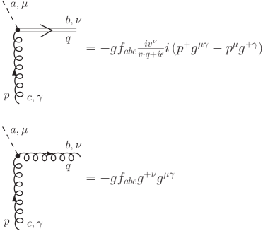
Figure 1: The Feynman rule for the TMD vertices. The first comes from the eikonal line and the second comes from the non-abelian term in the field strength tensor. In this calculation, the sum of the two will be lumped together and labelled by the gauge link.

II.2 One-loop Calculations Without Soft Factor

In this subsection, we calculate the unpolarized TMD gluon distribution in a gluon target in perturbative QCD to one-loop order, ignoring the soft contribution. According to the definition, the distribution is normalized to

$$g(x,k_{\perp})=\delta(x-1)\delta^{2}(k_{\perp})\ ,$$ (3)

at leading order. At one-loop order, we have both virtual and real corrections. We regulate the infrared (soft) divergences using dimensional regularization. Moreover, we introduce the off-shellness for the initial gluon, $p^{2}<0$, to regulate possible collinear divergences.

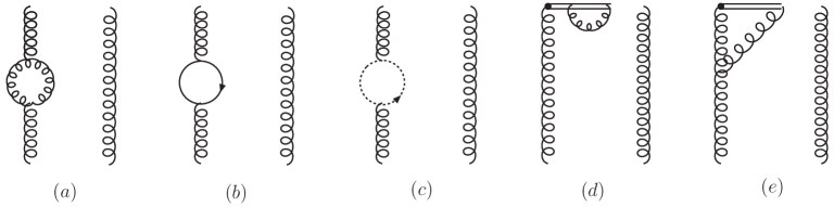
Figure 2: Virtual corrections to the TMD gluon distribution at one-loop order. The mirror diagrams are not shown.

The one-loop virtual diagrams are shown in Fig. 2, which are the self-energy diagrams for the gluon wave function and from the gauge link, and the vertex corrections. The contribution from Figs. 2(a), (b) and (c) has the form

$$g(x,k_{\perp})|_{\rm fig.2(a-c)}=\delta(x-1)\delta^{2}(k_{\perp})(Z_{G}-1)\ ,$$ (4)

where

$$Z_{G}=1+\frac{\alpha_{s}}{4\pi}\left[-\ln\frac{-p^{2}}{\mu^{2}}\left(\frac{5}{3}C_{A}-\frac{2}{3}N_{f}\right)+\frac{31}{9}C_{A}-\frac{10}{9}N_{f}\right]\$$ (5)

A factor of 2 has been included to account for the contributions from the conjugate diagrams. Here $C_{A}=N_{c}$, and $N_{f}$ is the number of the active quark flavors. Minimal subtraction has been made to remove the UV divergence. Collinear divergence is indicated by the dependence on the off-shellness of the gluon.

The contribution from Fig. 2(d) has the similar form, $\delta(x-1)\delta^{2}(k_{\perp})(Z_{W}-1)$, with

$$Z_{W}=1+\frac{\alpha_{s}C_{A}}{2\pi}\left[-\frac{2}{\epsilon_{\rm IR}}+\gamma_{E}+\ln\frac{1}{4\pi}\right]\ ,$$ (6)

where $1/\epsilon_{\rm IR}$ ($\epsilon_{\rm IR}=4-d$) pole comes from the soft divergence.

The contribution from Fig. 2(e) is $\delta(x-1)\delta^{2}(k_{\perp})(Z_{V}-1)$ with

$$Z_{V} = 1-\frac{\alpha_{s}C_{A}}{2\pi}\left[-\frac{4}{\epsilon_{\rm IR}^{2}}-\frac{2}{\epsilon_{\rm IR}}\left(\ln\frac{\zeta^{2}}{4\pi\mu^{2}}-2\ln\frac{-p^{2}}{4\pi\mu^{2}}-\gamma_{E}\right)+\frac{1}{2}\left(\ln^{2}\frac{\zeta^{2}}{4\pi\mu^{2}}-2\ln^{2}\frac{-p^{2}}{4\pi\mu^{2}}\right)\right.$$ (7)

$$~{}~{}\left.+\gamma_{E}\left(\ln\frac{\zeta^{2}}{4\pi\mu^{2}}-2\ln\frac{-p^{2}}{4\pi\mu^{2}}\right)-\ln\frac{\zeta^{2}}{-p^{2}}-\frac{1}{2}\ln\frac{\zeta^{2}}{\mu^{2}}+\frac{3}{2}-\frac{\gamma_{E}^{2}}{2}+\frac{7\pi^{2}}{12}\right]\ .$$

Here we have taken the limit $\zeta^{2}=(2v\cdot P)^{2}/v^{2}$ is much larger than any soft scale (e.g. $-p^{2}$). The result shows explicitly the double logarithmic dependence of the TMD distribution on $\zeta^{2}$. These double logarithms can be resummed using the Collins-Soper evolution equation, which will be discussed in Sec. IIE. The total contribution from the virtual diagrams is

$$g(x,k_{\perp},\mu,x\zeta)|_{\rm virtual}=\delta(x-1)\delta^{2}(k_{\perp})\left(Z_{G}+Z_{W}+Z_{V}-3\right)\ .$$ (8)

Again the virtual correction contains soft divergences.

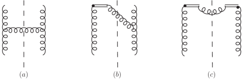
Figure 3: Same as Fig. 2 but for the real contributions.

Now we turn to the real corrections shown in Fig. 3. The contribution from Fig. 3(a) is

$$g(x,k_{\perp})|_{\rm fig.3(a)}=\frac{\alpha_{s}C_{A}}{\pi^{2}}\frac{1}{k_{\perp}^{2}-x(1-x)p^{2}}\left[\frac{1-x}{x}+x(1-x)+\frac{x}{2}\right]\ .$$ (9)

Fig. 3(b) contributes

$$g(x,k_{\perp},x\zeta)|_{\rm fig.3(b)}=\frac{\alpha_{s}C_{A}}{\pi^{2}}\left\{\frac{1}{k_{\perp}^{2}-x(1-x)p^{2}}\left[\frac{x}{(1-x)_{+}}-\frac{x}{2}\right]+\frac{1}{2}\frac{\mu^{\epsilon}}{k_{\perp}^{2}}\ln\frac{\zeta^{2}}{k_{\perp}^{2}}\delta(x-1)\right\}\ ,$$ (10)

where a factor of 2 has been included to account for the mirror diagrams. The plus function follows the definition in AltPar77 . The limit of $\zeta^{2}\rightarrow\infty$ has been taken whenever there is no divergence. The contribution from Fig. 3(c) can be calculated similarly,

$$g(x,k_{\perp})|_{\rm fig.3(c)}=-\frac{\alpha_{s}C_{A}}{2\pi^{2}}\frac{\mu^{\epsilon}}{k_{\perp}^{2}}\delta(x-1)\$$ (11)

The above contributions contain soft divergences as indicated by the $1/k_{\perp}^{2}$ term as $k_{\perp}^{2}\rightarrow 0$. We have to keep the pre-factors of these terms up to ${\cal O}(\epsilon)$, which can lead to finite contributions after Fourier transforming into the impact parameter $b$-space. The soft divergences from the real and virtual diagrams will eventually cancel, as we shall see.

II.3 Soft Factor

As in the case of TMD quark distributions, there are soft contributions from Figs. 2 and 3, signaled by soft divergences. These contributions can be extracted using the well-known Grammer-Yennie approximation GraYen73 . Here we follow the same procedure as for the quark distributions JiMaYu04 , and define the soft factor

$$S(b,\mu,\rho)=\frac{1}{(N_{c}^{2}-1)}\langle 0|{\cal L}_{\bar{v}cb^{\prime}}^{\dagger}(b_{\perp};-\infty){\cal L}_{vb^{\prime}a}^{\dagger}(-\infty;b_{\perp}){\cal L}_{vab}(0;-\infty){\cal L}_{\bar{v}bc}(-\infty;0)|\rangle\ ,$$ (12)

where $\bar{v}$ is another off-light-cone vector, $\bar{v}=(\bar{v}^{-},\bar{v}^{+},0)$ with $\bar{v}^{+}\gg\bar{v}^{-}$, and $\rho$ is defined as $\rho^{2}=v^{-}\bar{v}^{+}/v^{+}\bar{v}^{-}$. The same soft factor will appear in the factorization of semi-inclusive scalar particle production we shall see in Sec. IV.

At one-loop order, we have diagrams shown in Fig. 4 which are the same as those considered in JiMaYu04 , except for the color factor. Here we use dimensional regularization for the infrared divergence instead of a gluon mass. The final result is the same because the soft factor is free of infrared divergences.

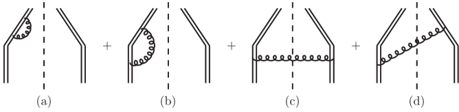
Figure 4: Soft contributions to the TMD gluon distribution at one-loop order.

The contribution from Fig. 4(a) is

$$\triangle_{\rm soft}g(x,k_{\perp})|_{\rm fig.4(a)}=-2\delta(x-1)\delta^{2}(k_{\perp})(Z_{W}-1)\ ,$$ (13)

where $Z_{W}$ is in Eq. (6). The contribution from Fig. 4(b) is

$$\triangle_{\rm soft}g(x,k_{\perp})|_{\rm fig.4(b)}=\delta(x-1)\delta^{2}(k_{\perp})\frac{\alpha_{s}C_{A}}{2\pi}\ln\rho^{2}\left(-\frac{2}{\epsilon_{\rm IR}}+\gamma_{E}+\ln\frac{1}{4\pi}\right)\ ,$$ (14)

where the UV divergence has been subtracted using $\overline{\rm MS}$ scheme. The contribution from Fig. 4(c) is

$$\triangle_{\rm soft}g(x,k_{\perp})|_{\rm fig.4(c)}=\delta(x-1)\frac{\alpha_{s}C_{A}}{\pi^{2}}\frac{\mu^{\epsilon}}{k_{\perp}^{2}}\ .$$ (15)

Fig. 4(d) gives,

$$\triangle_{\rm soft}g(x,k_{\perp})|_{\rm fig.4(d)}=-\delta(x-1)\frac{\alpha_{s}C_{A}}{2\pi^{2}}\ln\rho^{2}\frac{\mu^{\epsilon}}{k_{\perp}^{2}}\ .$$ (16)

The individual diagrams all have infrared divergences. However, they all cancel eventually. For example, the IR divergence from Fig. 4(a) cancels that from (c), while that in (b) cancels that in (d). The cancellation can best be seen from the impact parameter $b$-space expression. After Fourier transformation, we get

$$\triangle_{\rm soft}g(x,b,\mu,x\zeta,\rho)=\delta(x-1)\frac{\alpha_{s}C_{A}}{2\pi}\ln\left(\frac{\mu^{2}b^{2}}{4}e^{2\gamma_{E}}\right)\left[\ln\rho^{2}-2\right]\$$ (17)

We thus confirm that it is the same soft factor as in the quark distributions JiMaYu04 , except for the color factor.

We note that there are different definitions of the soft factor in the literature JiMaYu04 ; ColMet04 ; ColHau00 . The difference can be viewed as the scheme dependence. Final physical results do not depend on a particular definition.

II.4 TMD Gluon Distribution at One-Loop

Summarizing the results from the last two subsections, we get the gluon TMD distribution at one-loop order,

$$g(x,k_{\perp},\mu,x\zeta,\rho) = \delta(x-1)\delta^{2}(k_{\perp})\left[Z_{G}+Z_{V}-2+(Z_{W}-1)(\ln\rho^{2}-1)\right]$$ (18)

$$+\delta(x-1)\frac{\alpha_{s}C_{A}}{2\pi^{2}}\frac{\mu^{\epsilon}}{k_{\perp}^{2}}\left(\ln\frac{\zeta^{2}}{k_{\perp}^{2}}-\ln\rho^{2}+1\right)$$

$$+\frac{\alpha_{s}C_{A}}{\pi^{2}}\frac{1}{k_{\perp}^{2}-x(1-x)p^{2}}\left[\frac{x}{(1-x)_{+}}+\frac{1-x}{x}+x(1-x)\right]\ .$$

The individual terms have soft divergences which cancel out in the sum. In the impact parameter $b$-space, we define

$$g(x,b,\mu,x\zeta)=\int d^{2}k_{\perp}e^{i\vec{k}_{\perp}\cdot\vec{b}_{\perp}}g(x,k_{\perp},\mu,x\zeta)\$$ (19)

After Fourier transformation,

$$g(x,b,\mu,x\zeta) = \frac{\alpha_{s}C_{A}}{\pi}\left(\ln\frac{4}{-p^{2}b^{2}}-2\gamma_{E}\right)\left[\frac{x}{(1-x)_{+}}+\frac{1-x}{x}+x(1-x)\right]$$ (20)

$$~{}~{}+\frac{\alpha_{s}C_{A}}{\pi}\left[\left(\frac{x}{1-x}\ln\frac{1}{x(1-x)}\right)_{+}+\ln\frac{1}{x(1-x)}\left(\frac{1-x}{x}+x(1-x)\right)\right]$$

$$~{}~{}+\delta(x-1)\left\{\left(Z_{G}-1\right)+\frac{\alpha_{s}C_{A}}{2\pi}\left[-\frac{1}{2}\ln^{2}\left(\frac{\zeta^{2}b^{2}}{4}e^{2\gamma_{E}}\right)-\ln\frac{-p^{2}b^{2}}{4}e^{2\gamma_{E}}\right.\right.$$

$$~{}~{}\left.\left.+\ln\frac{\zeta^{2}b^{2}}{4}e^{2\gamma_{E}}+\ln\frac{\mu^{2}b^{2}}{4}e^{2\gamma_{E}}\left(\ln\rho^{2}-1\right)+\frac{1}{2}\ln\frac{\zeta^{2}}{\mu^{2}}-\frac{\pi^{2}}{2}-\frac{11}{2}\right]\right\}\ .$$

The $1/\epsilon_{\rm IR}$ poles have now disappeared. However, there are still collinear divergences as indicated by the dependence on $\ln(-p^{2})$. More interestingly, we have double logarithmic dependence on $\zeta^{2}$, the energy of the parenting gluon. We study this dependence in the next subsection.

II.5 Collins-Soper Evolution in Hadron Energy

From the above result, we see that the TMD gluon distribution depends on the energy of the parenting hadrons, through the variable $\zeta^{2}=(2v\dot{P})^{2}/v^{2}\approx 2(P^{+})^{2}v^{-}/v^{+}$. The energy evolution of the TMD parton distribution is controlled by the Collins-Soper evolution equation ColSop81 . In impact-parameter space, the Collins-Soper equation reads as

$$\zeta\frac{\partial}{\partial\zeta}g(x,b,x\zeta,\mu,\rho)=(K_{g}+G_{g})g(x,b,x\zeta,\mu,\rho)\ ,\$$ (21)

where $K$ and $G$ are soft and hard evolution kernels, respectively.

It is easy to check that the one-loop TMD gluon distribution indeed satisfies the Collins-Soper equation. The sum of $K+G$ can be extracted,

$$K_{g}+G_{g}=-\frac{\alpha_{s}C_{A}}{\pi}\ln\frac{x^{2}\zeta^{2}b^{2}}{4}e^{2\gamma_{E}-\frac{3}{2}}\ .$$ (22)

The soft part $K$ can be calculated from a definition similar to the quark case Col89 ; JiMaYu043 ,

$$K_{g}=-\frac{\alpha_{s}C_{A}}{\pi}\ln\frac{\mu^{2}b^{2}}{4}e^{2\gamma_{E}}\ ,$$ (23)

and thus the hard part $G_{g}$ can be solved from the sum. The $K$ and $G$ obey the renormalization group equation,

$$\mu\frac{\partial K_{g}}{\partial\mu}=-\mu\frac{\partial G_{g}}{\partial\mu}=-\gamma_{Kg}=-2\frac{\alpha_{s}C_{A}}{\pi}\$$ (24)

These evolution equations will be used to resum the large logarithms in the cross section in Sec. V.

III TMD Parton Distributions at Large Transverse Momentum

As emphasized in JiMaYu04 , it is nontrivial to generate the integrated (Feynman) parton distributions by integrating out the transverse momentum in the TMD distributions. The main difficulty is that new ultraviolet divergences emerge from the transverse momentum integration. However, there is another way to connect the two distributions ColSop81p : When the transverse momentum becomes large or the impact parameter becomes small, part of the TMD distributions are calculable from perturbative QCD, because at least one hard gluon is needed to generate the large momentum. The hard-gluon radiation leads to power-like behavior, e.g. $1/k_{\perp}^{2}$, for the unpolarized TMD distributions. Here Feynman parton distributions enter as the non-perturbative input in the QCD factorization analysis.

We consider the Fourier-transformed version of TMD distributions at small $b$. The factorization theorem reads ColSop81 ; ColSop81p ,

$$f_{i}(x,b,\mu,x\zeta,\rho)=\sum_{j}\int\frac{dy}{y}\tilde{C}_{i/j}\left(\frac{x}{y},\mu,\zeta,b,\bar{\mu}\right)f_{j}(y,\bar{\mu})\ ,$$ (25)

where $i,~{}j$ denote the flavor of the partons—quarks and gluons. The integrated distributions $f_{j}$ on the right-hand side depend on the longitudinal momentum fraction $x$ and the scale $\bar{\mu}$. $\tilde{C}_{i/j}$ are the coefficient functions and are calculable from perturbative QCD. In the following, we will verify the above formula and extract the coefficient functions at one-loop order.

We choose an on-shell quark target (with mass $m$) and an off-shell gluon target (with off-shellnes $p^{2}$) to regulate the collinear divergences. We need to calculate both the TMD and integrated parton distributions up to one-loop order. The collinear divergences in both distributions must be matched, and the subtracted coefficient functions are free of infrared divergences.

The coefficient functions $\tilde{C}_{i/j}$ have perturbation expansions in terms of the strong coupling constant $\alpha_{s}$. At leading order ($\alpha_{s}^{0}$), it is easy to see,

$$\tilde{C}_{q/q}^{(0)} = \tilde{C}_{g/g}^{(0)}=\delta(x-1)\ ,$$

$$\tilde{C}_{g/q}^{(0)} = \tilde{C}_{q/g}^{(0)}=0\ .$$ (26)

At one-loop, all receive non-trivial contributions. $\tilde{C}_{q/q}$ has been calculated before in JiMaYu04 , where a gluon mass was used to regulate the soft divergences. We have checked this calculation by using dimensional regularization and obtained the same result. For completeness, we quote the result here,

$$\tilde{C}_{q/q}^{(1)}\left(x,b^{2},\mu^{2},\bar{\mu}^{2},x^{2}\zeta^{2},\rho\right)$$

$$=\frac{\alpha_{s}}{2\pi}C_{F}\left\{(1-x)+\left(\frac{1+x^{2}}{1-x}\right)_{+}\ln\frac{4}{b^{2}\bar{\mu}^{2}}e^{-2\gamma_{E}}\right.$$

$$\left.+\delta(x-1)\left[\left(\frac{1}{2}-\ln\rho^{2}\right)\ln\frac{4}{b^{2}\mu^{2}}e^{-2\gamma_{E}}-\frac{1}{2}\ln^{2}\left(\frac{\zeta^{2}b^{2}}{4}e^{2\gamma_{E}-1}\right)-\frac{3+\pi^{2}}{2}\right]\right\}\ .$$ (27)

To calculate $\tilde{C}_{g/g}^{(1)}$, we need the integrated gluon distribution at one loop,

$$g^{(1)}(x,\bar{\mu}) = \frac{\alpha_{s}C_{A}}{\pi}\left\{\ln\frac{\bar{\mu}^{2}}{-p^{2}}{\cal P}_{gg}(x)+\left(\frac{x}{1-x}\ln\frac{1}{x(1-x)}\right)_{+}-\delta(x-1)\left(1-\frac{31}{36}+\frac{5N_{f}}{54}\right)\right.$$ (28)

$$~{}~{}~{}~{}~{}~{}~{}\left.+\left(\frac{1-x}{x}+x(1-x)\right)\ln\frac{1}{x(1-x)}\right\}\ ,$$

where ${\cal P}_{gg}(x)$ is the gluon splitting function,

$${\cal P}_{gg}(x)=\frac{x}{(1-x)_{+}}+\frac{1-x}{x}+x(1-x)+\delta(x-1)\beta_{0}\ ,$$ (29)

with $\beta_{0}=(11-2/3N_{f})/12$. From the above and one-loop TMD gluon distribution, the coefficient function for the gluon-gluon term is

$$\tilde{C}_{g/g}^{(1)}\left(x,b^{2},\mu^{2},\bar{\mu}^{2},x^{2}\zeta^{2},\rho\right)$$

$$=\frac{\alpha_{s}C_{A}}{\pi}\left\{{\cal P}_{gg}(x)\ln\frac{4}{b^{2}\bar{\mu}^{2}}e^{-2\gamma_{E}}+\delta(x-1)\left[\left(\beta_{0}+\ln\rho-\frac{1}{2}\right)\ln\frac{b^{2}\mu^{2}}{4}e^{2\gamma_{E}}\right.\right.$$

$$\left.\left.+\frac{3}{4}\ln\frac{\zeta^{2}}{\mu^{2}}-\frac{1}{4}\ln^{2}\left(\frac{\zeta^{2}b^{2}}{4}e^{2\gamma_{E}}\right)-\frac{\pi^{2}+7}{4}\right]\right\}\ ,$$ (30)

where the collinear divergences of the form $\ln(-p^{2})$ have been cancelled.

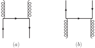
Figure 5: Quark splitting to gluon contribution to $\tilde{C}_{g/q}$ (a) and gluon splitting to quark $\tilde{C}_{q/g}$ (b).

The Feynman diagrams for the quark-gluon and gluon-quark splitting coefficient functions $\tilde{C}_{g/q}$ and $\tilde{C}_{q/g}$ are shown in Fig. 5(a) and (b). The TMD gluon distribution in a quark target is

$$g(x,k_{\perp})|_{\rm fig.5(a)}=\frac{\alpha_{s}C_{F}}{2\pi^{2}}\left[\frac{1+(1-x)^{2}}{x}\frac{1}{k_{\perp}^{2}+m^{2}}-\frac{2x(1-x)m^{2}}{(k_{\perp}^{2}+x^{2}m^{2})^{2}}\right]\ .$$ (31)

After Fourier-transforming into the impact parameter $b$-space, we have,

$$g(x,b)|_{\rm fig.5(a)}=\frac{\alpha_{s}C_{F}}{2\pi}\left[\frac{1+(1-x)^{2}}{x}\ln\left(\frac{4}{m^{2}b^{2}x^{2}}e^{-2\gamma_{E}}\right)-\frac{2(1-x)}{x}\right]\ .$$ (32)

The corresponding integrated gluon distribution is,

$$g(x,\bar{\mu})|_{\rm fig.5(a)}=\frac{\alpha_{s}C_{F}}{2\pi}\left[\frac{1+(1-x)^{2}}{x}\ln\frac{\bar{\mu}^{2}}{m^{2}x^{2}}-\frac{2(1-x)}{x}-x\right]\ .$$ (33)

Combining the above, we find the coefficient function,

$$\tilde{C}_{g/q}^{(1)}\left(x,b^{2},\bar{\mu}^{2}\right)=\frac{\alpha_{s}C_{F}}{2\pi}\left[\frac{1+(1-x)^{2}}{x}\ln\left(\frac{4}{b^{2}\bar{\mu}^{2}}e^{-2\gamma_{E}}\right)+x\right]\ .$$ (34)

Similarly, we find the coefficient function for finding a quark in a gluon target,

$$\tilde{C}_{q/g}^{(1)}\left(x,b^{2},\bar{\mu}^{2}\right)=\frac{\alpha_{s}}{4\pi}\left[\left(x^{2}+(1-x)^{2}\right)\ln\left(\frac{4}{b^{2}\bar{\mu}^{2}}e^{-2\gamma_{E}}\right)+2x(1-x)\right]\ .$$ (35)

These calculations can certainly be carried out to higher orders in $\alpha_{s}$.

IV Scalar-particle production through gluon fusion

It is difficult to study the gluon TMD distributions in semi-inclusive DIS because gluons do not have direct couplings with photons, and their contributions are power suppressed JiMaYu04 . However, we can access these distributions at hadron colliders through, for example, the heavy-quark pair or di-jet production. In these processes, the total transverse momentum of the pair or the di-jet provides information on the TMD parton distributions in the initial hadrons, and the gluon distributions could dominate at some kinematics.

An important question we have to address is the factorization of the QCD radiative corrections. Only when the factorization is established can we safely extract the TMD parton distributions from data. In this section, we will consider QCD factorization for the gluon initiated processes, with scalar-particle production as an example. The scalar particle here has a direct coupling to the gluons through an effective vertex. The transverse-momentum distribution of the produced scalars reflect partly the transverse-momentum dependence of the gluon densities in the nucleon. Our study can be extended to other gluon initiated semi-inclusive processes at hadron colliders.

The effective lagrangian for the gluon-scalar coupling is,

$${\cal L}_{eff}=-\frac{1}{4}g_{\phi}\Phi F^{a}_{\mu\nu}F^{a\mu\nu}\ ,$$ (36)

where $\Phi$ is the scalar field and $g_{\phi}$ is the effective coupling. For the standard model Higgs boson, the effective coupling can be derived from the full theory Ellis75 ; Shifman:1979eb . The above effective lagrangian has also been used Mueller:1989st to study the gluon saturation in nuclei.

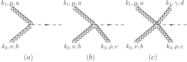
Figure 6: Vertices for the scalar particle coupling to the gluons. All labelled momenta are in.

From the above lagrangian, we can write down the basic vertices for the scalar particle coupling to the gluon potentials, shown in Fig. 6. The Feynman rule for the coupling with two gluons in Fig. 6(a) is

$$ig_{\phi}\delta_{ab}\left(k_{1}\cdot k_{2}g_{\mu\nu}-k_{1\nu}k_{2\mu}\right)\ .$$ (37)

And the coupling with three gluons in Fig. 6(b) reads

$$-g_{\phi}g_{s}f_{abc}\left[(k_{1}-k_{2})_{\rho}g_{\mu\nu}+(k_{2}-k_{3})_{\mu}g_{\rho\nu}+(k_{3}-k_{1})_{\nu}g_{\rho\mu}\right]\ .$$ (38)

Finally, the coupling with four gluons shown in Fig. 6(c) is

$$-ig_{\phi}g_{s}^{2} \left\{\right. f_{abe}f_{cde}\left(g_{\mu\rho}g_{\nu\gamma}-g_{\mu\gamma}g_{\nu\rho}\right)$$ (39)

$$+ f_{ace}f_{bde}\left(g_{\mu\nu}g_{\rho\gamma}-g_{\mu\gamma}g_{\nu\rho}\right)$$

$$+ \left.f_{ade}f_{bce}\left(g_{\mu\nu}g_{\rho\gamma}-g_{\mu\rho}g_{\nu\gamma}\right)\right\}\ .$$

Production of a single scalar particle has a cross section linear in $g_{\phi}^{2}$. We are interested in higher-order QCD corrections in $\alpha_{s}$.

Scalar-particle production at low transverse momentum depends on the TMD gluon distributions of the incident hadrons. A new feature for semi-inclusive processes is the dependence on the soft factor ColSop81 ; JiMaYu04 . In a factorized form, the cross section can be written as a product of the TMD parton distributions (or fragmentation functions), the soft factor $S$, and the hard factor $H$ ColSop81 ; JiMaYu04 ,

$$\frac{d^{3}\sigma(M^{2},P_{\perp},y)}{d^{2}P_{\perp}dy} = \sigma_{0}\int d^{2}k_{1\perp}d^{2}k_{2\perp}d^{2}\ell_{\perp}x_{1}g(x_{1},k_{1\perp},x_{1}\zeta_{1},\mu,\rho)x_{2}g(x_{2},k_{2\perp},x_{2}\zeta_{2},\mu,\rho)$$ (40)

$$\times S(\ell_{\perp},\mu,\rho)H(M^{2},\mu,\rho)\delta^{2}(\vec{k}_{1\perp}+\vec{k}_{2\perp}+\vec{\ell}_{\perp}-\vec{P}_{\perp})\ ,$$

where $\sigma_{0}$ is the leading-order scalar-particle production from two gluons,

$$\sigma_{0}=\frac{\pi g_{\phi}^{2}}{64}\frac{1}{1-\epsilon/2}\ .$$ (41)

Here the factor $(1-\epsilon/2)$ in the denominator comes from the polarization average of the initial gluons. The hard scale $M$ here denotes the mass of the scalar particle, and $y$ and $P_{\perp}$ are its rapidity and transverse momentum, respectively. At low-transverse momentum, the longitudinal-momentum fractions $x_{1}$ and $x_{2}$ for the two incident gluons can be approximately related to the scalar particle’s rapidity $y$ through $x_{1}=\sqrt{M^{2}/S}e^{y}$ and $x_{2}=\sqrt{M^{2}/S}e^{-y}$, where $S$ is the total center-of-mass energy squared $S=(P_{1}+P_{2})^{2}$. $\zeta_{1}$ and $\zeta_{2}$ are defined as $\zeta_{1}^{2}=4(v\cdot P_{1})/v^{2}$ and $\zeta_{2}^{2}=4(\bar{v}\cdot P_{2})/\bar{v}^{2}$, and $v$ and $\bar{v}$ are defined in the last section. $\rho$ as defined before, is a parameter to separate gluon contributions to the soft and hard factors.

The above factorization result is accurate at the leading power in $P_{\perp}^{2}/M^{2}$ at low transverse momentum. In the following, we will examine this factorization formula up to one-loop order using the perturbative TMD gluon distributions from the previous section. Through explicit computation, we obtain the one-loop result for the hard factor $H$. For arguments toward a factorization to all orders, we follow the discussion in ColSop81 ; JiMaYu04 .

In principle, the above factorization formula works only at the low transverse momentum region, and it breaks down at $P_{\perp}\sim M$, where one can no longer neglect the power corrections of $P_{\perp}^{2}/M^{2}$. However, it is useful to extrapolate the above factorization to all $P_{\perp}$, and convert it to the impact-parameter space. After Fourier transformation, the differential cross section can be written as,

$$\frac{d^{3}\sigma(M^{2},P_{\perp},y)}{d^{2}P_{\perp}dy} = \sigma_{0}\int\frac{d^{2}\vec{b}}{(2\pi)^{2}}e^{-iP_{\perp}\cdot b_{\perp}}W(x_{1},x_{2},b,M^{2})\ ,$$ (42)

where we define

$$W(x_{1},x_{2},b,Q^{2})=x_{1}g(x_{1},b,x_{1}\zeta_{1},\mu,\rho)x_{2}g(x_{2},b,x_{2}\zeta_{2},\mu,\rho)S(b,\mu,\rho)H(M^{2},\mu,\rho)\ .$$ (43)

The convolutions in the transverse-momentum space now reduce to products in the impact parameter $b$-space.

IV.1 Factorization At One Loop

In this subsection, we calculate the scalar-particle production to one-loop order to verify the factorization, and to extract the hard factor $H$. The gluon TMD distributions and soft factor have been calculated in Sec.II, where the gluon target has been put off-shell (by nonzero $-p^{2}$). In this section, it is more convenient to demonstrate the factorization by using the on-shell gluon target ($p^{2}=0$). It is straightforward to extend the results in Sec.II to the on-shell case. In the new scheme, the perturbative TMD gluon distribution is,

$$g(x,b,x\zeta,\mu,\rho) = \delta(x-1)$$ (44)

$$+\frac{\alpha_{s}C_{A}}{\pi}\left\{{\cal P}_{gg}(x)\left(-\frac{2}{\epsilon_{\rm IR}}-\gamma_{E}+\ln\frac{4}{4\pi\mu^{2}b^{2}}\right)\right.$$

$$~{}~{}~{}~{}\left.+\delta(x-1)\left[\left(\ln\rho+\beta_{0}-\frac{1}{2}\right)\ln\frac{b^{2}\mu^{2}}{4}e^{2\gamma_{E}}-\frac{1}{4}\ln^{2}\left(\frac{\zeta^{2}b^{2}}{4}e^{2\gamma_{E}}\right)\right.\right.$$

$$~{}~{}~{}~{}\left.\left.+\frac{3}{4}\ln\frac{\zeta^{2}}{\mu^{2}}-\frac{\pi^{2}+7}{4}\right]\right\}\ .$$

Here, $1/\epsilon_{\rm IR}$ indicates collinear divergence. The soft factor $S(b,\mu,\rho)$ was defined in Eq. (12). At one loop, the result in impact parameter space is

$$S(b,\mu,\rho)=\frac{\alpha_{s}C_{A}}{2\pi}\ln\left(\frac{b^{2}\mu^{2}}{4}e^{2\gamma_{E}}\right)\left(2-\ln\rho^{2}\right)\ .$$ (45)

These results will be used to verify the above factorization formula.

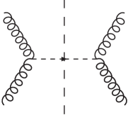
Figure 7: Scalar particle production at leading order.

At leading order, the Born diagram for the production cross section is shown in Fig.7. The calculation is straightforward, and we get

$$\frac{d\sigma}{d^{2}P_{\perp}dy}=\frac{\pi g_{\phi}^{2}}{64}\delta(x_{1}-1)\delta(x_{2}-1)\delta^{2}(P_{\perp})\ .$$ (46)

This leads to

$$W^{(0)}(x_{i},b)=\delta(x_{1}-1)\delta(x_{2}-1)\ ,$$ (47)

which can be clearly reproduced by the leading-order gluon distributions in gluon targets

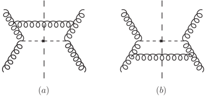
Figure 8: Real diagrams contribution to the scalar particle production through gluon fusion: part I.

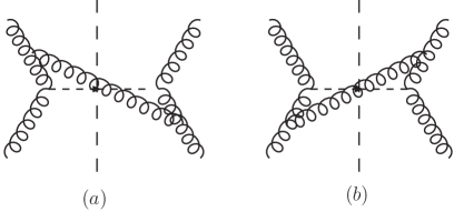
Figure 9: Real diagrams: part II.

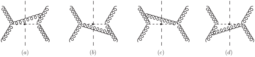
Figure 10: Real diagrams: part III.

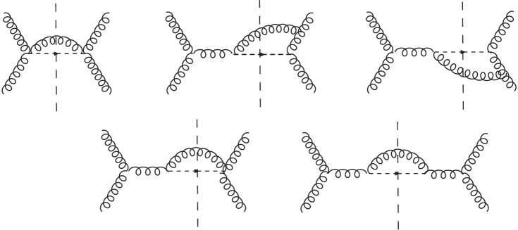
Figure 11: Power suppressed real diagrams.

At next-to-leading order, we have both real and virtual contributions. The real diagrams are shown in Figs. (8-11). Figure 8 represents the contributions from the gluon radiation from either gluons, while Fig. 9 for the interference between these radiations. Figure 10 includes the diagrams involving the three-gluon coupling with the scalar particle. The contribution from Fig. 8 is

$$\left.\frac{d\sigma}{d^{2}P_{\perp}dy}\right|_{\rm fig.8}=\sigma_{0}\frac{C_{A}\alpha_{s}}{\pi^{2}}\frac{\mu^{\epsilon}}{P_{\perp}^{2}}\left\{x_{1}\left[\frac{1-x_{1}}{x_{1}}+x_{1}(1-x_{1})+\frac{x_{1}}{2}\right]\delta(x_{2}-1)+(x_{1}\leftrightarrow x_{2})\right\}\$$ (48)

In the above result, we have kept the pre-factor up to ${\cal O}(\epsilon)$, because $1/P_{\perp}^{2}$ will lead to infrared divergences when Fourier-transforming to the impact parameter space. The contribution from Fig.  9 is,

$$\left.\frac{d\sigma}{d^{2}P_{\perp}dy}\right|_{\rm fig.9} = \sigma_{0}\frac{C_{A}\alpha_{s}}{\pi^{2}}\frac{\mu^{\epsilon}}{P_{\perp}^{2}}\left\{\left[\left(\frac{x_{1}}{(1-x_{1})_{+}}-\frac{x_{1}}{2}\right)+\frac{1}{2}\ln\frac{M^{2}}{P_{\perp}^{2}}\delta(x_{1}-1)\right]\delta(x_{2}-1)\right.$$ (49)

$$\left.+(x_{1}\leftrightarrow x_{2})\right\}\ ,$$

and the contribution from all diagrams in Fig. 10 is,

$$\left.\frac{d\sigma}{d^{2}P_{\perp}dy}\right|_{\rm fig.10} = \sigma_{0}\frac{C_{A}\alpha_{s}}{\pi^{2}}\frac{\mu^{\epsilon}}{P_{\perp}^{2}}\left\{\left(-\frac{x_{1}^{2}+x_{1}}{2}\right)\delta(x_{2}-1)+(x_{1}\leftrightarrow x_{2})\right\}\ .$$ (50)

The diagrams in Fig. 11 are power-suppressed at low-transverse momentum, although their contributions are leading when the transverse momentum is on the order of $M$. The sum of the contributions from all the real diagrams is

$$\left.\frac{d\sigma}{d^{2}P_{\perp}dy}\right|_{\rm real} = \sigma_{0}\frac{C_{A}\alpha_{s}}{\pi^{2}}\frac{\mu^{\epsilon}_{\rm IR}}{P_{\perp}^{2}}\left\{\left[x_{1}\left(\frac{x_{1}}{(1-x_{1})_{+}}+\frac{1-x_{1}}{x_{1}}+x_{1}(1-x_{1})\right)\right.\right.$$ (51)

$$\left.\left.+\frac{1}{2}\ln\frac{M^{2}}{P_{\perp}^{2}}\delta(x_{1}-1)\right]\delta(x_{2}-1)+(x_{1}\leftrightarrow x_{2})\right\}\ .$$

The above agrees with a corresponding result in Ref. Kauffman:1991jt . After Fourier-transforming to the impact parameter space, one finds,

$$W^{(1)}(x_{i},b,M^{2})|_{\rm real} = \frac{\alpha_{s}C_{A}}{\pi}\left\{\left[\left(-\frac{2}{\epsilon_{\rm IR}}-\gamma_{E}+\ln\frac{4}{4\pi\mu^{2}b^{2}}\right)\delta(x_{2}-1)x_{1}\left(\frac{x_{1}}{(1-x_{1})_{+}}\right.\right.\right.$$ (52)

$$\left.\left.+x_{1}(1-x_{1}+\frac{1-x_{1}}{x_{1}})\right)+(x_{1}\rightarrow x_{2})\right]$$

$$\left.+\delta(x_{1}-1)\delta(x_{2}-1)\left[\frac{4}{\epsilon^{2}_{\rm IR}}\right.-\frac{2}{\epsilon_{\rm IR}}\left(\ln\frac{M^{2}}{4\pi\mu^{2}}+\gamma_{E}\right)+\frac{1}{2}\ln^{2}\left(\frac{M^{2}}{4\pi\mu^{2}}\right)\right.$$

$$\left.\left.-\frac{1}{2}\ln^{2}\left(\frac{M^{2}b^{2}}{4}e^{2\gamma_{E}}\right)+\gamma_{E}\ln\frac{M^{2}}{4\pi\mu^{2}}+\frac{\gamma_{E}^{2}}{2}-\frac{\pi^{2}}{12}\right]\right\}\ .$$

The double and single poles above correspond to infrared divergences only.

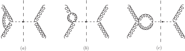
Figure 12: Virtual diagrams contribution to the scalar particle production through gluon fusion.

Now we turn to the virtual diagrams shown in Fig. 12. These diagrams contribute to the cross section as Dawson:1990zj ; Djouadi:1991tk

$$W(x_{i},b,M^{2})|_{\rm virtual} = \delta(x_{1}-1)\delta(x_{2}-1)\frac{\alpha_{s}C_{A}}{\pi}\left[-\frac{4}{\epsilon^{2}}+\frac{2}{\epsilon}\left(\ln\frac{M^{2}}{4\pi\mu^{2}}+\gamma_{E}\right)-\frac{1}{2}\ln^{2}\left(\frac{M^{2}}{4\pi\mu^{2}}\right)\right.$$ (53)

$$\left.-\gamma_{E}\ln\frac{M^{2}}{4\pi\mu^{2}}-\frac{\gamma_{E}^{2}}{2}+\frac{7\pi^{2}}{12}\right]\$$

The $1/\epsilon^{2}$ pole above cancels that from the real diagrams. The above result has ultra-violet divergences which comes from the composite gluon operator in the effective coupling. This divergence can be cancelled by a charge renormalization contribution,

$$W(x_{i},b,M^{2})|_{\rm charge}=\frac{\alpha_{s}C_{A}}{\pi}2\beta_{0}\left(\frac{M^{2}}{4\pi\mu^{2}}\right)^{-\epsilon/2}\left(-\frac{2}{\epsilon}+\gamma_{E}\right)\delta(x_{1}-1)\delta(x_{2}-1)\ .$$ (54)

where the extra factor is introduced so that renormalization scale is set at $\mu_{UV}^{2}=M^{2}$. The gluon wave function renormalization constant $Z_{A}=1$ to all orders in perturbation theory in the present scheme. By summing up all the contributions, we get $W(x_{i},b,M^{2})$ at one-loop order,

$$W^{(1)}(x_{i},b,Q^{2}) = \frac{\alpha_{s}C_{A}}{\pi}\left\{\left[x_{1}{\cal P}_{gg}(x_{1})\delta(x_{2}-1)\left(-\frac{2}{\epsilon}-\gamma_{E}+\ln\frac{4}{4\pi\mu^{2}b^{2}}\right)+(x_{1}\rightarrow x_{2})\right]\right.$$

$$+\left.\delta(x_{1}-1)\delta(x_{2}-1)\left[2\beta_{0}\ln\frac{b^{2}M^{2}}{4}e^{2\gamma_{E}}-\frac{1}{2}\ln^{2}\left(\frac{M^{2}b^{2}}{4}e^{2\gamma_{E}}\right)+\frac{\pi^{2}}{2}\right]\right\}\ .$$

The soft divergences have been cancelled between real and virtual diagrams, and there are remaining collinear divergences.

Now we can verify the factorization formula in Eqs. (40), (43), using the one-loop results in Eqs. (44), (45). After the subtractions, we obtain the hard factor at one loop,

$$H^{(1)}(M^{2},\mu^{2},\rho) = \frac{\alpha_{s}C_{A}}{\pi}\left[\ln\frac{M^{2}}{\mu^{2}}\left(2\beta_{0}+\frac{1}{2}\ln\rho^{2}-\frac{3}{2}\right)-\frac{3}{4}\ln\rho^{2}+\frac{1}{8}\ln^{2}\rho^{2}+\pi^{2}+\frac{7}{2}\right]\ ,$$

where a special coordinate system has been chosen: $x_{1}^{2}\zeta_{1}^{2}=x_{2}^{2}\zeta_{2}^{2}=\rho M^{2}$. Not only the collinear divergences in the cross section have been cancelled by the gluon distributions, the $b$-dependence has also been entirely isolated in the parton distributions and soft factor. The hard factor $H$ depends only on the hard scale $M^{2}$, the factorization scale $\mu$, and the parameter $\rho$. Thus, the factorization conjectured in Eq. (40) is verified to one-loop order. Furthermore, according to the general arguments provided in ColSop81 ; JiMaYu04 , all-order QCD corrections to scalar-particle production can be factorized in a similar way.

IV.2 Factorization at Small $b\ll 1/\Lambda_{\rm QCD}$

When $b$ is small, there is the standard QCD factorization in terms of Feynman parton distributions for $W(x_{i},b,M^{2})$ ColSopSte85 . In this subsection, we will try to recover this factorization, using the results in the last subsection.

According to ColSopSte85 , the cross section $W(x_{i},b,M^{2})$ at small $b$ can be written as,

$$W(x_{i},b,M^{2})=\int\frac{d\xi_{1}}{\xi_{1}}\frac{d\xi_{2}}{\xi_{2}}\xi_{1}g(\xi_{1},\mu)\xi_{2}g(\xi_{2},\mu)C_{gg}(\frac{x_{1}}{\xi_{1}},b,\mu,M^{2})C_{gg}(\frac{x_{2}}{\xi_{2}},b,\mu,M^{2})\ ,$$ (57)

where $g(x,\mu)$ is the usual gluon distribution, and the coefficient functions $C_{gg}$ is perturbative. They both depend on the factorization scale $\mu$, but the dependence cancels out in the product.

Using $W(x_{i},b,M^{2})$ from the last subsection, we can calculate the $C_{gg}$ to one-loop. The perturbative gluon distribution up to one-loop is

$$g(x)=\delta(x-1)+\frac{\alpha_{s}C_{A}}{\pi}{\cal P}_{gg}(x)\left(-\frac{2}{\epsilon}+\gamma_{E}+\ln\frac{1}{4\pi}\right)\ .$$ (58)

Subtracting the above from the one-loop $W(x_{i},b,M^{2})$, we have

$$C_{gg}(x,b,\mu,M^{2}) = \delta(x-1)+\frac{\alpha_{s}C_{A}}{\pi}\left\{x{\cal P}_{gg}(x)\ln\left(\frac{4}{b^{2}\mu^{2}}e^{-2\gamma_{E}}\right)\right.$$ (59)

$$\left.+\delta(x-1)\left[\beta_{0}\ln\left(\frac{b^{2}M^{2}}{4}e^{2\gamma_{E}}\right)-\frac{1}{4}\ln^{2}\left(\frac{M^{2}b^{2}}{4}e^{2\gamma_{E}}\right)+\frac{\pi^{2}}{4}\right]\right\}\ .$$

The $\mu$-dependence of the $C_{gg}$ function is controlled by the same evolution equation as for the gluon distribution, with the opposite sign. When $b^{2}M^{2}$ is large, one needs to re-sum the large double logarithms to all orders in perturbation theory. This is difficult to do systematically in the present formalism. However, this can be done straightforwardly in terms of the TMD factorization in the previous subsection.

V Resummation of Large Double Logarithms

The one-loop result for scalar-particle production shows that there exists large double logarithms in the hard scale $M^{2}$ (e.g., see Eq. (LABEL:higgstotal)). These large logarithms appear at every order of the perturbative expansion, $\alpha_{s}^{n}\ln^{2m}M^{2}/P_{\perp}^{2}$ where $m\leq n$ and $P_{\perp}$ is the transverse momentum. In order to make reliable predictions, one has to re-sum these large logarithms. In this section, we will follow the Collins-Soper-Sterman (CSS) framework ColSopSte85 to perform the resummation. The results can be used as a double check of the resummation studies in the literature for the standard model Higgs production at hadron colliders Hinchliffe:1988ap ; Kauffman:1991jt ; Yuan:1991we .

V.1 Collins-Soper-Sterman Resummation at Small b

According to the QCD factorization, the Fourier transformation of the cross section for scalar-particle production is

$$W(x_{i},b,M^{2})=x_{1}g(x_{1},b,\mu,\rho M^{2},\rho)x_{2}g(x_{2},b,\mu,\rho M^{2},\rho)S(b,\mu,\rho)H(M^{2},\rho,\mu)\$$ (60)

In the above equation we have set $x_{1}^{2}\zeta_{1}^{2}=x_{2}^{2}\zeta_{2}^{2}=\rho M^{2}$ in a special frame of coordinates. The $M^{2}$ dependence of $W$ can be studied through the following differential equation ColSopSte85 ,

$$\frac{\partial W(x_{i},b,M^{2})}{\partial\ln M^{2}}=(K+G^{\prime})W(x_{i},b,M^{2})\ ,$$ (61)

where $K$ and $G^{\prime}$ are soft and hard evolution kernels. The soft part $K$ depends on the scale $1/b^{2}$ and the renormalization scale $\mu$, while $G^{\prime}$ depends on the hard scale $M^{2}$ and $\mu$. $K$ can be calculated from the Collins-Soper evolution equation for the TMD gluon distributions discussed in Sec.IID. $G^{\prime}$ contains the contributions from the gluon distribution as well as from the hard factor $H$. From the result of the previous sections, the sum of $K$ and $G^{\prime}$ at one-loop order is,

$$K+G^{\prime}=-\frac{\alpha_{s}C_{A}}{\pi}\ln\left(\frac{M^{2}b^{2}}{4}e^{2\gamma_{E}-2\beta_{0}}\right)\ ,$$ (62)

where the $\rho$ dependence between various terms cancels out. Our previous result for $K$ at one loop is

$$K=K_{g}=-\frac{\alpha_{s}C_{A}}{\pi}\ln\frac{b^{2}\mu^{2}}{4}e^{2\gamma_{E}}\ ,$$ (63)

which is valid when $b$ is small enough. At large $b$, the perturbative expansion breaks down. The hard part $G^{\prime}$ is,

$$G^{\prime}=-\frac{\alpha_{s}C_{A}}{\pi}\left(\ln\frac{M^{2}}{\mu^{2}}-2\beta_{0}\right)\ .$$ (64)

Both the soft and hard parts $K$ and $G^{\prime}$ also obey the renormalization group equation ColSopSte85 ,

$$\frac{\partial K}{\partial\ln\mu}=-\frac{\partial G^{\prime}}{\partial\ln\mu}=-\gamma_{Kg}\ .$$ (65)

Resummation is done here by solving the above equations.

Integrating over $\ln M^{2}$ and $\ln\mu^{2}$, one finds ColSopSte85

$$W(x_{i},b,M^{2})=e^{-{\cal S}_{Sud}(M^{2},b,C_{1}/C_{2})}W(x_{i},b,C_{1}^{2}/C_{2}^{2}/b^{2})\ ,$$ (66)

where the Sudakov form factor is

$${\cal S}_{Sud}=\int_{C_{1}^{2}/b^{2}}^{C_{2}^{2}M^{2}}\frac{d\mu^{2}}{\mu^{2}}\left[\ln\left(\frac{C_{2}^{2}M^{2}}{\mu^{2}}\right)A(C_{1},\mu)+B(C_{1},C_{2},\mu)\right]\ .$$ (67)

Here $C_{1}$ and $C_{2}$ are two parameters of order one. The functions $A$ and $B$ can be expanded perturbatively $\alpha_{s}$, $A=\sum\limits_{i=1}^{\infty}A^{(i)}\left(\frac{\alpha_{s}}{\pi}\right)^{i}$ and $B=\sum\limits_{i=1}^{\infty}B^{(i)}\left(\frac{\alpha_{s}}{\pi}\right)^{i}$. They are related to the Collins-Soper evolution parameters by the following equation,

$$A(C_{1},\mu) = \frac{1}{2}\gamma_{Kg}(\mu)+\frac{1}{2}\beta\frac{\partial}{\partial g}K(C_{1},g(\mu))\ ,$$

$$B(C_{1},C_{2},\mu) = -K(C_{1},g(\mu))-G^{\prime}(1/C_{2},g(\mu))\ .$$ (68)

From Eqs. (63,64), we get the first expansion of $A$ and $B$ functions,

$$A^{(1)}=C_{A},~{}~{}~{}B^{(1)}=C_{A}\left[\ln\left(\frac{C_{1}^{2}}{4C_{2}^{2}}e^{2\gamma_{E}}\right)-2\beta_{0}\right]\ .$$ (69)

To complete the resummation, we use the factorization of $W(x_{i},b,C_{1}^{2}/C_{2}^{2}/b^{2})$ in terms of the integrated parton distributions discussed in Sec. IVB,

$$W\left(x_{i},b,\frac{C_{1}^{2}}{C_{2}^{2}b^{2}}\right) = \int\frac{d\xi_{1}}{\xi_{1}}\frac{d\xi_{2}}{\xi_{2}}C_{gg}\left(\frac{x_{1}}{\xi_{1}},b;\frac{C_{1}^{2}}{C_{2}^{2}b^{2}},\mu^{2}\right)C_{gg}\left(\frac{x_{2}}{\xi_{2}},b;\frac{C_{1}^{2}}{C_{2}^{2}b^{2}},\mu^{2}\right)$$ (70)

$$\times\xi_{1}g(\xi_{1},\mu)\xi_{2}g(\xi_{2},\mu)\ ,$$

where $C$ functions also have perturbation expansion in terms of $\alpha_{s}$, $C=\sum\limits_{i=0}^{\infty}C^{(i)}\left(\frac{\alpha_{s}}{\pi}\right)^{i}$. From the results in Sec. IVB, we get the first two terms of $C_{gg}$,

$$C_{gg}^{(0)} = \delta(x-1)$$

$$C_{gg}^{(1)} = C_{A}\left\{x{\cal P}_{gg}(x)\ln\left(\frac{4}{C_{1}^{2}}e^{-2\gamma_{E}}\right)\right.$$ (71)

$$~{}~{}~{}\left.+\delta(x-1)\left[\beta_{0}\ln\left(\frac{C_{1}^{2}}{4C_{2}^{2}}e^{2\gamma_{E}}\right)-\frac{1}{4}\ln^{2}\left(\frac{C_{1}^{2}}{4C_{2}^{2}}e^{2\gamma_{E}}\right)+\frac{\pi^{2}}{4}\right]\right\}\ .$$

It is easy to check that the above $C$ function for the gluon-gluon term can also be calculated from the following equation JiMaYu04

$$C_{gg}(x,b;\frac{C_{1}^{2}}{C_{2}^{2}b^{2}},\mu^{2})=x\tilde{C}_{gg}\left(x,b^{2},\mu_{g}^{2},\mu^{2},\rho\frac{C_{1}^{2}}{C_{2}^{2}b^{2}},\rho\right)\times\sqrt{S(b,\mu_{g}^{2},\rho)H(\frac{C_{1}^{2}}{C_{2}^{2}b^{2}},\mu_{g}^{2},\rho)}\ ,$$ (72)

with $\tilde{C}_{gg}$ from Eq.(30), and $S$ and $H$ from Eqs. (45), (LABEL:hardh) respectively. Similarly, the contribution from the quark distribution in the factorization form of Eq. (70) can also be calculated using the above equation with $\tilde{C}_{g/q}$ in Eq. (34). Since $\tilde{C}_{g/q}^{(0)}=0$, it is straightforward to get the expansion of $C_{g/q}$ up to one-loop order,

$$C_{g/q}^{(0)} = 0$$

$$C_{g/q}^{(1)} = \frac{C_{F}}{2}x\left[\frac{1+(1-x)^{2}}{x}\ln\left(\frac{4}{b^{2}\mu^{2}}e^{-2\gamma_{E}}\right)+x\right]\ .$$ (73)

Our final resummation result is the combination of Eqs. (66), (67), (70), (71) and (73).

V.2 Comparison with Previous Calculations

In the literature, the above coefficient functions have also been calculated by various authors Catani:1988vd ; Hinchliffe:1988ap ; Kauffman:1991jt ; Yuan:1991we . They are normally extracted from the comparison between the fixed-order results and the expansion of the resummation formula, and expressed with the so-called canonical parameters, with $C_{1}=2e^{-\gamma_{E}}$ and $C_{2}=1$. Choosing these specific values, our results for $A$, $B$, $C$ at one-loop order are,

$$A^{(1)}=C_{A},~{}~{}~{}B^{(1)}=-2\beta_{0}C_{A},~{}~{}~{}C_{gg}^{(1)}=C_{A}\frac{\pi^{2}}{4}\delta(x-1)\ .$$ (74)

$A^{(1)}$ and $B^{(1)}$ agree with the previous calculations Catani:1988vd ; Hinchliffe:1988ap ; Kauffman:1991jt , while $C^{(1)}$ lacks an additional term $11/4$. The difference comes from the effective coupling between the Higgs boson and gluons $g_{\phi}$ Dawson:1990zj ; Djouadi:1991tk

$$g_{H}=-\frac{1}{3{\cal V}}\frac{\alpha_{s}}{\pi}\left[1+\frac{11}{4}\frac{\alpha_{s}}{\pi}+\cdots\right]\ ,$$ (75)

where ${\cal V}$ is the vacuum expectation value of the Higgs field. The second term will contribute at one-loop order in $\alpha_{s}$ and modify the result of Eq. (53). Taking this into account, our results coincide with the previous calculations Hinchliffe:1988ap ; Kauffman:1991jt .

In Yuan:1991we , the full of dependence on $C_{1}$ and $C_{2}$ of the coefficient functions were also calculated for the standard model Higgs boson production. Our result on $B^{(1)}$ agrees with theirs, while $C^{(1)}$ does not .

VI Conclusion

In this paper, we have studied scalar-particle production at one-loop order to examine the factorization of the gluon initiated semi-inclusive processes at hadron colliders. We introduced and calculated the gauge-invariant TMD gluon distribution at one-loop order, and established their connections with the integrated parton distributions at small $b$. We verified the factorization theorem at one-loop order, where the cross section can be decomposed into products of TMD parton distributions, soft and hard factors. The large logarithms in the cross section were resummed following the CSS formalism, and the coefficient functions were obtained. The factorization to all orders in QCD coupling is assumed following the general arguments in ColSop81 ; JiMaYu04 .

The present study can be easily extended to the polarized gluon TMD distributions and their contributions to the spin asymmetries for the semi-inclusive processes. Scalar-particle production can also be generalized to other production processes, e.g., heavy-quark pairs and heavy quarkonium production, di-photon and di-hadron and photon-hadron production, and di-jet correlations. We will carry out further studies in future publications.

The present study of factorization for semi-inclusive processes can be extended to two-loop order, which can be used to compare with the NNLO calculation of the standard model Higgs production. It will be interesting to calculate the resummation coefficient functions from the present approach, and compare with the previous results obtained by the expansion method deFlorian:2000pr .

As a final remark, we consider the small-$x$ property of the gluon TMD distributions. From the results in Sec.II, we found that the TMD gluon distribution at small $x$ has the similar behavior as the integrated gluon distribution, where the small $x$ resummation is usually necessary. The so-called BFKL evolution equation Lipatov:1976zz is usually used to make the resummation. It will be interesting to examine whether the TMD gluon distributions obey such evolution equation at small $x$ Sterman:1995fz , and to explore the connection between the present approach and the so-called $k_{t}$-factorization approach Col91 . Phenomenologically, the small-$x$ effects are important for the Higgs boson and vector-boson production at LHC Berge:2004nt .

References

- (1) J. C. Collins and D. E. Soper, Nucl. Phys. B 193, 381 (1981) [Erratum-ibid. B 213, 545 (1983)]; Nucl. Phys. B 197, 446 (1982).
- (2) J. C. Collins and D. E. Soper, Nucl. Phys. B 194, 445 (1982).
- (3) J. C. Collins, D. E. Soper and G. Sterman, Nucl. Phys. B 250, 199 (1985).
- (4) R. Meng, F. I. Olness and D. E. Soper, Phys. Rev. D 54, 1919 (1996) [arXiv:hep-ph/9511311].
- (5) P. Nadolsky, D. R. Stump and C. P. Yuan, Phys. Rev. D 61, 014003 (2000) [Erratum-ibid. D 64, 059903 (2001)] [arXiv:hep-ph/9906280]; Phys. Rev. D 64, 114011 (2001) [arXiv:hep-ph/0012261].
- (6) J. P. Ralston and D. E. Soper, Nucl. Phys. B 152, 109 (1979).
- (7) J. C. Collins, Nucl. Phys. B 396, 161 (1993) [arXiv:hep-ph/9208213].
- (8) D. W. Sivers, Phys. Rev. D 41, 83 (1990); Phys. Rev. D 43, 261 (1991).
- (9) M. Anselmino, M. Boglione and F. Murgia, Phys. Lett. B 362, 164 (1995) [arXiv:hep-ph/9503290]; M. Anselmino and F. Murgia, Phys. Lett. B 442, 470 (1998) [arXiv:hep-ph/9808426].
- (10) P. J. Mulders and R. D. Tangerman, Nucl. Phys. B 461, 197 (1996) [Erratum-ibid. B 484, 538 (1997)] [arXiv:hep-ph/9510301]; D. Boer and P. J. Mulders, Phys. Rev. D 57, 5780 (1998) [arXiv:hep-ph/9711485].
- (11) S. J. Brodsky, D. S. Hwang and I. Schmidt, Phys. Lett. B 530, 99 (2002) [arXiv:hep-ph/0201296].
- (12) J. C. Collins, Phys. Lett. B 536, 43 (2002) [arXiv:hep-ph/0204004]; Acta Phys. Polon. B 34, 3103 (2003) [arXiv:hep-ph/0304122].
- (13) X. Ji and F. Yuan, Phys. Lett. B 543, 66 (2002) [arXiv:hep-ph/0206057]. A. V. Belitsky, X. Ji and F. Yuan, Nucl. Phys. B 656, 165 (2003) [arXiv:hep-ph/0208038];
- (14) D. Boer, P. J. Mulders and F. Pijlman, Nucl. Phys. B 667, 201 (2003) [arXiv:hep-ph/0303034].
- (15) X. Ji, J. P. Ma and F. Yuan, Phys. Rev. D 71, 034005 (2005) [arXiv:hep-ph/0404183].
- (16) X. Ji, J. P. Ma and F. Yuan, Phys. Lett. B 597, 299 (2004) [arXiv:hep-ph/0405085].
- (17) J. C. Collins and A. Metz, Phys. Rev. Lett. 93, 252001 (2004) [arXiv:hep-ph/0408249].
- (18) P. J. Mulders and J. Rodrigues, Phys. Rev. D 63, 094021 (2001) [arXiv:hep-ph/0009343].
- (19) M. Burkardt, Phys. Rev. D 69, 091501 (2004) [arXiv:hep-ph/0402014].
- (20) D. Boer and W. Vogelsang, Phys. Rev. D 69, 094025 (2004) [arXiv:hep-ph/0312320].
- (21) M. Anselmino, M. Boglione, U. D’Alesio, E. Leader and F. Murgia, Phys. Rev. D 70, 074025 (2004) [arXiv:hep-ph/0407100].
- (22) J. C. Collins, D. E. Soper and G. Sterman, Nucl. Phys. B 263, 37 (1986); Nucl. Phys. B 308, 833 (1988).
- (23) J. C. Collins, D. E. Soper and G. Sterman, Adv. Ser. Direct. High Energy Phys. 5, 1 (1988); in Perturbative QCD (A.H. Mueller, ed.) (World Scientific Publ., 1989).
- (24) Y. L. Dokshitzer, D. Diakonov and S. I. Troian, Phys. Lett. B 78, 290 (1978); Phys. Lett. B 79, 269 (1978); Phys. Rept. 58, 269 (1980).
- (25) G. Parisi and R. Petronzio, Nucl. Phys. B 154, 427 (1979).
- (26) G. Sterman, Nucl. Phys. B 281, 310 (1987).
- (27) S. Catani and L. Trentadue, Nucl. Phys. B 327, 323 (1989); Nucl. Phys. B 353, 183 (1991).
- (28) J. R. Ellis, M. K. Gaillard and D. V. Nanopoulos, Nucl. Phys. B 106, 292 (1976).
- (29) M. A. Shifman, A. I. Vainshtein, M. B. Voloshin and V. I. Zakharov, Sov. J. Nucl. Phys. 30, 711 (1979) [Yad. Fiz. 30, 1368 (1979)].
- (30) S. Dawson, Nucl. Phys. B 359, 283 (1991).
- (31) A. Djouadi, M. Spira and P. M. Zerwas, Phys. Lett. B 264, 440 (1991).
- (32) M. Kramer, E. Laenen and M. Spira, Nucl. Phys. B 511, 523 (1998) [arXiv:hep-ph/9611272].
- (33) R. V. Harlander and W. B. Kilgore, Phys. Rev. Lett. 88, 201801 (2002) [arXiv:hep-ph/0201206].
- (34) C. Anastasiou and K. Melnikov, Nucl. Phys. B 646, 220 (2002) [arXiv:hep-ph/0207004].
- (35) S. Catani, E. D’Emilio and L. Trentadue, Phys. Lett. B 211, 335 (1988).
- (36) I. Hinchliffe and S. F. Novaes, Phys. Rev. D 38, 3475 (1988).
- (37) R. P. Kauffman, Phys. Rev. D 44, 1415 (1991); Phys. Rev. D 45, 1512 (1992).
- (38) C. P Yuan, Phys. Lett. B 283, 395 (1992); C. Balazs and C. P. Yuan, Phys. Lett. B 478, 192 (2000) [arXiv:hep-ph/0001103]; Phys. Rev. D 63, 014021 (2001) [arXiv:hep-ph/0002032].
- (39) D. de Florian and M. Grazzini, Phys. Rev. Lett. 85, 4678 (2000) [arXiv:hep-ph/0008152]; Nucl. Phys. B 616, 247 (2001) [arXiv:hep-ph/0108273].
- (40) E. L. Berger and J. W. Qiu, Phys. Rev. D 67, 034026 (2003) [arXiv:hep-ph/0210135]; Phys. Rev. Lett. 91, 222003 (2003) [arXiv:hep-ph/0304267].
- (41) G. Bozzi, S. Catani, D. de Florian and M. Grazzini, Phys. Lett. B 564, 65 (2003) [arXiv:hep-ph/0302104].
- (42) A. Kulesza, G. Sterman and W. Vogelsang, Phys. Rev. D 69, 014012 (2004) [arXiv:hep-ph/0309264].
- (43) J. C. Collins, Adv. Ser. Direct. High Energy Phys. 5, 573 (1989) [arXiv:hep-ph/0312336]; in Perturbative QCD (A.H. Mueller, ed.) (World Scientific Publ., 1989).
- (44) G. Altarelli and G. Parisi, Nucl. Phys. B 126, 298 (1977).
- (45) G. J. Grammer and D. R. Yennie, Phys. Rev. D 8, 4332 (1973).
- (46) A. Idilbi, X. Ji, J. P. Ma and F. Yuan, Phys. Rev. D 70, 074021 (2004) [arXiv:hep-ph/0406302].
- (47) J. C. Collins and F. Hautmann, Phys. Lett. B 472, 129 (2000) [arXiv:hep-ph/9908467]; JHEP 0103, 016 (2001) [arXiv:hep-ph/0009286].
- (48) A. H. Mueller, Nucl. Phys. B 335, 115 (1990).
- (49) L. N. Lipatov, Nonabelian Sov. J. Nucl. Phys. 23, 338 (1976) [Yad. Fiz. 23, 642 (1976)]; E. A Kuraev, L. N. Lipatov and V. S. Fadin, Sov. Phys. JETP 44, 443 (1976) [Zh. Eksp. Teor. Fiz. 71, 840 (1976)]; E. A Kuraev, L. N. Lipatov and V. S. Fadin, Sov. Phys. JETP 45, 199 (1977) [Zh. Eksp. Teor. Fiz. 72, 377 (1977)]; I. I. Balitsky and L. N. Lipatov, Sov. J. Nucl. Phys. 28, 822 (1978) [Yad. Fiz. 28, 1597 (1978)].
- (50) G. Sterman, arXiv:hep-ph/9606312.
- (51) J. C. Collins and R. K. Ellis, Nucl. Phys. B 360, 3 (1991); S. Catani, M. Ciafaloni and F. Hautmann, Nucl. Phys. B 366, 135 (1991).
- (52) S. Berge, P. Nadolsky, F. Olness and C. P. Yuan, arXiv:hep-ph/0410375.