Abstract

In this article, we study the magnetic moment of the pentaquark state $\Theta^{+}(1540)$ as diquark-diquark-antiquark ($[ud][ud]\bar{s}$) state with the QCD sum rules in the external weak electromagnetic field (EFSR) and the light-cone QCD sum rules (LCSR) respectively. The numerical results indicate the magnetic moment is about $\mu_{\Theta^{+}}=-(0.11\pm 0.02)\mu_{N}$ for the EFSR and $\mu_{\Theta^{+}}\approx-(0.1-0.5)\mu_{N}$ for the LCSR. As the values obtained from the EFSR are more stable than the corresponding ones from the LCSR, $\mu_{\Theta^{+}}=-(0.11\pm 0.02)\mu_{N}$ is more reliable.

PACS : 12.38.Aw, 12.38.Lg, 12.39.Ba, 12.39.-x

Key Words: QCD Sum Rules, Magnetic moment, Pentaquark

1 Introduction

The observation of the new baryon state $\Theta^{+}(1540)$ with positive strangeness and minimal quark content $udud\bar{s}$ [1] has motivated intense theoretical investigations to clarify the quantum numbers and to understand the under-structures of the exotic state [2, 3]. Although the pentaquark state $\Theta^{+}(1540)$ can be signed to the top of the antidecuplet $\overline{10}$ with isospin $I=0$, the spin and parity have not been experimentally determined yet and no consensus has ever been reached on the theoretical side [2, 3]. The discovery has opened a new field of strong interaction and provides a new opportunity for a deeper understanding of the low energy QCD especially when multiquark states are involved. The magnetic moments of the pentaquark states are fundamental parameters as their masses, which have copious information about the underlying quark structures, can be used to distinguish the preferred configurations from various theoretical models and deepen our understanding of the underlying dynamics. Furthermore, the magnetic moment of the pentaquark state $\Theta^{+}(1540)$ is an important ingredient in studying the cross sections of the photo- or electro-production, which can be used to determine the fundamental quantum number of the pentaquark state $\Theta^{+}(1540)$, such as spin and parity [4, 8], and may be extracted from experiments eventually in the future.

There have been several works on the magnetic moments of the pentaquark state $\Theta^{+}(1540)$ [5, 6, 7, 8, 9, 10, 11, 12, 13, 14, 15], in this article, we take the point of view that the baryon $\Theta^{+}(1540)$ is a diquark-diquark-antiquark ($[ud][ud]\bar{s}$) state with the quantum numbers $J=\frac{1}{2}$ , $I=0$ , $S=+1$, and study its magnetic moment with the QCD sum rules in the external weak electromagnetic field (EFSR) and the light-cone QCD sum rules (LCSR) respectively [16, 17, 18]. Different quark configurations can be implemented with different interpolating currents, if the $u$ and $d$ quarks in the pentaquark state $\Theta^{+}(1540)$ are bound into spin zero, color and flavor antitriplet $\bar{3}$ diquarks, we can take the diquarks (for example, $\epsilon^{abc}u_{b}C\gamma_{5}d_{c}$ with $J^{P}=0^{+}$ and $\epsilon^{abc}u_{b}Cd_{c}$ with $J^{P}=0^{-}$ ) instead of the $u$ and $d$ quarks as the basic constituents to construct the interpolating currents.

The article is arranged as follows: we derive the EFSR and LCSR for the magnetic moment of the pentaquark state $\Theta^{+}(1540)$ in section II; in section III, numerical results and discussions; section IV is reserved for conclusion.

2 EFSR and LCSR

Although for medium and asymptotic momentum transfers the operator product expansion approach can be applied for the form factors and moments of wave functions, at low momentum transfer, the standard operator product expansion approach cannot be consistently applied, as pointed out in the early work on photon couplings at low momentum for the nucleon magnetic moments [17]. In Ref.[17], the problem was solved by using a two-point correlation function in an external electromagnetic field, with vacuum susceptibilities introduced as parameters for nonperturbative propagation in the external field, i.e. the QCD sum rules in the external field. As nonperturbative vacuum properties, the susceptibilities can be introduced for both small and large momentum transfers in the external fields. The alternative way is the light-cone QCD sum rules, which was firstly used to calculate the magnetic moments of the nucleons in Ref.[19]. For more discussions about the magnetic moments of the baryons in the framework of the LCSR approach, one can consult Ref.[20].

In the following, we write down the two-point correlation functions $\Pi_{EF\eta}(p)$ and $\Pi_{LC\eta}(p)$ for the EFSR and LCSR respectively [21],

$$\Pi_{EF\eta}(p) = i\int d^{4}xe^{ip\cdot x}\langle 0|T\{\eta(x){\bar{\eta}}(0)\}|0\rangle_{F_{\mu\nu}}\,,$$ (1)

$$= \Pi_{0}(p)+\Pi_{\mu\nu}(p)F^{\mu\nu}+\cdots\,,$$

$$\Pi_{LC\eta}(p,q) = i\int d^{4}x\,e^{ipx}\langle\gamma(q)|T\{\eta(x)\bar{\eta}(0)\}|0\rangle,$$ (2)

where

$$\eta_{1}(x) = {1\over\sqrt{2}}\epsilon^{abc}\left\{\left[u_{a}^{T}(x)C\gamma_{5}d_{b}(x)\right]\left[u_{c}^{T}(x)C\gamma_{5}d_{e}(x)\right]C\bar{s}^{T}_{e}(x)-(u\leftrightarrow d)\right\},$$ (3)

$$\eta_{2}(x) = {1\over\sqrt{2}}\epsilon^{abc}\left\{\left[u_{a}^{T}(x)Cd_{b}(x)\right]\left[u_{c}^{T}(x)Cd_{e}(x)\right]C\bar{s}^{T}_{e}(x)-(u\leftrightarrow d)\right\},$$ (4)

$$\eta(x) = \left\{t\eta_{1}(x)+\eta_{2}(x)\right\}.$$ (5)

Here the $\gamma(q)$ represents the external electromagnetic field $A_{\mu}(x)=\varepsilon_{\mu}e^{iq\cdot x}$, the $\varepsilon_{\mu}$ is the photon polarization vector and the field strength $F_{\mu\nu}(x)=i(\varepsilon_{\nu}q_{\mu}-\varepsilon_{\mu}q_{\nu})e^{iq\cdot x}$. The $\Pi_{0}(p)$ is the correlation function without the external field $F_{\mu\nu}$ and the $\Pi_{\mu\nu}(p)$ is the linear response term. The $a$, $b$, $c$ and $e$ are color indexes, the $C=-C^{T}$ is the charge conjugation operator, and the $t$ is an arbitrary parameter. The constituents $\epsilon^{abc}u_{b}^{T}(x)C\gamma_{5}d_{c}(x)$ represent the scalar diquarks with $J^{P}=0^{+}$ and $\epsilon^{abc}u_{b}^{T}(x)Cd_{c}(x)$ represent the pseudoscalar diquarks with $J^{P}=0^{-}$, we can denote the $\eta_{1}(x)$ and $\eta_{2}(x)$ by S-type and P-type interpolating current respectively according to the spin and parity of the constituent diquarks. They both belong to the antitriplet $\bar{3}$ representation of the color and flavor $SU(3)$ group, and can cluster together with diquark-diquark-antiquark structure to give the total spin and parity for the pentaquark state $\Theta^{+}(1540)$ $J^{P}={\frac{1}{2}}^{+}$ . The scalar diquarks correspond to the ${}^{1}S_{0}$ states of $ud$ quark system. The one-gluon exchange force and the instanton induced force can lead to significant attractions between the quarks in the $0^{+}$ channels [22]. The pseudoscalar diquarks do not have nonrelativistic limit, can be taken as the ${}^{3}P_{0}$ states.

At the level of hadronic degrees of freedom, the linear response term $\Pi_{\mu\nu}(p)$ can be written as

$$\Pi_{\mu\nu}(p)F^{\mu\nu}=i\int d^{4}xe^{ip\cdot x}\langle 0\,|\eta(x)\left\{-i\int d^{4}yA_{\mu}(y)J^{\mu}(y)\right\}\bar{\eta}(0)\,|\,0\rangle.$$ (6)

According to the basic assumption of current-hadron duality in the QCD sum rules approach [16], we insert a complete series of intermediate states satisfying the unitarity principle with the same quantum numbers as the current operator $\eta(x)$ into the correlation functions in Eq.(2) and Eq.(6) to obtain the hadronic representation. After isolating the double-pole terms of the lowest pentaquark states, we get the following results,

$$\Pi_{\mu\nu}(p)F^{\mu\nu} = -\int d^{4}x\int d^{4}y{d^{4}k\over(2\pi)^{4}}{d^{4}k^{\prime}\over(2\pi)^{4}}\sum_{ss^{\prime}}\frac{1}{m^{2}_{\Theta^{+}}-k^{2}-i\epsilon}\frac{1}{m^{2}_{\Theta^{+}}-{k^{\prime}}^{2}-i\epsilon}$$ (7)

$$e^{ip\cdot x}A_{\mu}(y)\langle 0|\eta(x)|ks\rangle\langle ks|J^{\mu}(y)|k^{\prime}s^{\prime}\rangle\langle k^{\prime}s^{\prime}|\bar{\eta}(0)|0\rangle+\cdots\,$$

$$= -F^{\mu\nu}f_{0}^{2}\frac{F_{1}(0)+F_{2}(0)}{4(m_{\Theta^{+}}^{2}-p^{2})^{2}}\{{\hat{p}}\sigma_{\mu\nu}+\sigma_{\mu\nu}{\hat{p}}\}+\cdots;$$

$$\Pi_{LC\eta}(p,q) = -f_{0}^{2}\varepsilon^{\mu}\frac{{\hat{p}}+m_{\Theta^{+}}}{p^{2}-m_{\Theta^{+}}^{2}}[F_{1}(q^{2})\gamma_{\mu}+\frac{i\sigma_{\mu\nu}q^{\nu}}{2m_{\Theta^{+}}}F_{2}(q^{2})]\frac{{\hat{p}}+{\hat{q}}+m_{\Theta^{+}}}{(p+q)^{2}-m_{\Theta^{+}}^{2}}+\cdots$$ (8)

$$= -\frac{f_{0}^{2}\left[F_{1}(q^{2})+F_{2}(q^{2})\right]}{(p^{2}-m_{\Theta^{+}}^{2})((p+q)^{2}-m_{\Theta^{+}}^{2})}{\hat{p}}{\hat{\varepsilon}}({\hat{p}}+{\hat{q}})+\cdots$$

$$= \Pi_{LC}(p,q)i\varepsilon_{\mu\nu\alpha\beta}\gamma_{5}\gamma^{\mu}\varepsilon^{\nu}q^{\alpha}p^{\beta}+\cdots.$$

Here we have used the fix-point gauge $x_{\mu}A^{\mu}(x)=0$, $A_{\mu}(y)=-{1\over 2}F_{\mu\nu}y^{\nu}$, and the definition $\langle 0|\eta(0)|\Theta^{+}(p)\rangle=f_{0}u(p)$. From the electromagnetic form factors $F_{1}(q^{2})$ and $F_{2}(q^{2})$ , we can obtain the magnetic moment of the pentaquark state $\Theta^{+}(1540)$,

$$\mu_{\Theta^{+}}=\left\{F_{1}(0)+F_{2}(0)\right\}\frac{e_{\Theta^{+}}}{2m_{\Theta^{+}}}.$$ (9)

The linear response term $\Pi_{\mu\nu}(p)$ in the weak external electromagnetic field $F_{\mu\nu}$ has three different Dirac tensor structures,

$$\Pi_{\mu\nu}(p)=\Pi_{EF}(p)\left\{\sigma_{\mu\nu}{\hat{p}}+{\hat{p}}\sigma_{\mu\nu}\right\}+\Pi_{1}(p)i\left\{p_{\mu}\gamma_{\nu}-p_{\nu}\gamma_{\mu}\right\}{\hat{p}}+\Pi_{2}(p)\sigma_{\mu\nu}\,.$$ (10)

The first structure has an odd number of $\gamma$-matrix and conserves chirality, the second and third have even number of $\gamma$-matrixes and violate chirality. In the original QCD sum rules analysis of the nucleon magnetic moments [17], the interval of dimensions (of the condensates) for the odd structure is larger than the interval of dimensions for the even structures, one may expect a better accuracy of the results obtained from the sum rules with the odd structure. In this article, the spin of the pentaquark state $\Theta^{+}(1540)$ is supposed to be $\frac{1}{2}$, just like the nucleon. As in our previous work [15], we can choose the first Dirac tensor structure $\left\{\sigma_{\mu\nu}{\hat{p}}+{\hat{p}}\sigma_{\mu\nu}\right\}$ for analysis. The phenomenological spectral density of the EFSR in Eq.(7) can written as,

$$\frac{\mbox{Im}\Pi_{EF}(s)}{\pi}={1\over 4}\{F_{1}(0)+F_{2}(0)\}f_{0}^{2}\delta^{\prime}(s-m_{\Theta^{+}}^{2})+C_{subtract}\delta(s-m_{\Theta^{+}}^{2})+\cdots\,,$$ (11)

where the first term corresponds to the magnetic moment of the pentaquark state $\Theta^{+}(1540)$, and is of double-pole. The second term comes from the electromagnetic transitions between the pentaquark state $\Theta^{+}(1540)$ and the excited states (or high resonances), and is of single-pole. Here we introduce the quantity $C_{subtract}$ to represent the electromagnetic transitions between the ground pentaquark state and the high resonances, it may have complex dependence on the energy $s$ and high resonance masses. However, we have no knowledge about the high resonances, even the existence of the ground pentaquark state $\Theta^{+}(1540)$ is not firmly established, which is in contrast to the conventional baryons, in those channels we can use the experimental data as a guide in constructing the phenomenological spectral densities [23]. In practical manipulations, we can take the $C_{subtract}$ as an unknown constant, and fitted to reproduce reliable values for the form factors $F_{1}(0)+F_{2}(0)$, we will revisit this subject in Eq.(19). The contributions from the higher resonances and continuum states are suppressed after Borel transform and not shown explicitly for simplicity. For the LCSR, we write down only the double-pole term explicitly in Eq.(8) which corresponds to the magnetic moment of the pentaquark state $\Theta^{+}(1540)$, and choose the tensor structure $\varepsilon_{\mu\nu\alpha\beta}\gamma_{5}\gamma^{\mu}\varepsilon^{\nu}q^{\alpha}p^{\beta}$ for analysis [5]. The contributions from the single-pole terms which concerning the excited and continuum states are suppressed after the double Borel transform, and not shown explicitly for simplicity.

The calculation of the operator product expansion in the deep Euclidean space-time region at the level of quark and gluon degrees of freedom is straightforward and tedious, here technical details are neglected for simplicity, once the analytical results are obtained, then we can express the correlation functions at the level of quark-gluon degrees of freedom into the following forms through dispersion relation,

$$\Pi_{EF}(P^{2}) = \frac{e_{s}}{\pi}\int_{m_{s}^{2}}^{s_{0}}ds\frac{{\rm Im}[A(s)]}{s+P^{2}}+e_{s}B(P^{2})+\cdots\,,$$ (12)

$$\Pi_{LC}(p,q) = e_{s}\int_{0}^{1}du\left\{\frac{1}{\pi}\int_{m_{s}^{2}}^{s_{0}}ds\frac{{\rm Im}[C(s)]}{s-up^{2}-(1-u)(p+q)^{2}}+D(p,q)\right\}+\cdots\,,$$ (13)

where

$$\frac{{\rm Im}[A(s)]}{\pi} = -\frac{(5t^{2}+2t+5)s^{4}}{2^{14}5!4!\pi^{8}}+\frac{(5t^{2}+2t+5)s^{3}m_{s}\chi\langle\bar{s}s\rangle}{2^{9}5!4!\pi^{6}}+\frac{(5+2t-7t^{2})s\langle\bar{q}q\rangle^{2}}{2^{9}3^{2}\pi^{4}}$$

$$-\frac{(5+2t-7t^{2})m_{s}\langle\bar{q}q\rangle^{2}\langle\bar{s}s\rangle\chi}{2^{7}3^{2}\pi^{2}}-\frac{(5t^{2}+2t+5)s^{2}}{2^{17}4!\pi^{6}}\langle\frac{\alpha_{s}GG}{\pi}\rangle,$$

$$B(P^{2}) = \frac{(5t^{2}+2t+5)\langle\bar{q}q\rangle^{4}}{2^{5}3^{3}P^{4}},$$

$$\frac{{\rm Im}[C(s)]}{\pi} = \frac{(5t^{2}+2t+5)s^{4}}{2^{12}5!4!\pi^{8}}-\frac{(5t^{2}+2t+5)s^{3}f\psi(u)}{2^{13}5!\pi^{6}}+\frac{(7t^{2}-2t-5)s\langle\bar{q}q\rangle^{2}}{2^{7}3^{2}\pi^{4}}$$

$$-\frac{(7t^{2}-2t-5)\langle\bar{q}q\rangle^{2}f\psi(u)}{2^{6}3\pi^{2}}+\frac{(5t^{2}+2t+5)s^{2}}{2^{15}4!\pi^{6}}\langle\frac{\alpha_{s}GG}{\pi}\rangle$$

$$-\frac{(5t^{2}+2t+5)sf\psi(u)}{2^{14}3\pi^{4}}\langle\frac{\alpha_{s}GG}{\pi}\rangle,$$

$$D(p,q) = -\frac{(5t^{2}+2t+5)\langle\bar{q}q\rangle^{4}}{2^{3}3^{3}\left(-up^{2}-(1-u)(p+q)^{2}\right)^{2}}.$$

From Eqs.(12-13), we can see that due to the special interpolating current $\eta(x)$ ( see Eqs.(3-5)), the $u$ and $d$ quarks which constitute the diquarks have no contributions to the magnetic moment though they have electromagnetic interactions with the external field, the net contributions to the magnetic moment come from the $s$ quark only, which is different significantly from the results obtained in Refs.[5, 15], where all the $u$, $d$ and $s$ quarks have contributions. In Refs.[5, 15], the diquark-triquark type interpolating current $J(x)$ is used,

$$J(x)={1\over\sqrt{2}}\epsilon^{abc}\left\{u^{T}_{a}(x)C\gamma_{5}d_{b}(x)\right\}\{u_{e}(x){\bar{s}}_{e}(x)i\gamma_{5}d_{c}(x)-d_{e}(x){\bar{s}}_{e}(x)i\gamma_{5}u_{c}(x)\}\,.$$ (14)

Although the diquark-diquark-antiquark type and diquark-triquark type configurations implemented by the interpolating currents $\eta(x)$ and $J(x)$ respectively can give satisfactory masses for the pentaquark state $\Theta^{+}(1540)$, the resulting magnetic moments are substantially different, once the magnetic moment can be extracted from the electro- or photo-production experiments, we can select the preferred configuration. In this article, we have neglected the contributions from the direct instantons as the effects are supposed to be small. In Ref.[24], the authors calculate the leading direct instanton contributions to the operator product expansion of the nucleon correlation function with the Ioffe current

$$J_{p}(x) = \epsilon^{abc}[u^{T}_{a}(x)C\gamma_{\alpha}u_{b}(x)]\gamma_{5}\gamma^{\alpha}d_{c}(x)$$

in an external electromagnetic field, and find the instanton contributions affect only the chiral odd sum rules which had previously been considered unstable. The general form of the proton current can be written as [25]

$$J_{p}(x,t) = \epsilon_{abc}\left\{\left[u_{a}^{T}(x)Cd_{b}(x)\right]\gamma_{5}u_{c}(x)+t\left[u_{a}^{T}(x)C\gamma_{5}d_{b}(x)\right]u_{c}(x)\right\},$$ (15)

in the limit $t=-1$, we recover the Ioffe current. In this article, we take the value of the $t$ to be $t=-1$ in Eq.(5). The pentaquark currents in Eqs.(3-5) have the analogous Dirac structure as the baryon current in Eq.(15), so the contributions from the direct instantons may not affect significantly about our analysis of the chiral even Dirac structure in Eq.(10). Furthermore, our previous work on the pentaquark mass using the interpolating current

$$J(x) = \epsilon^{abc}\epsilon^{def}\epsilon^{cfg}\{u_{a}^{T}(x)Cd_{b}(x)\}\{u_{d}^{T}(x)C\gamma_{5}d_{e}(x)\}C\bar{s}_{g}^{T}(x)$$

indicates the direct instantons have neglectable contributions [26]. The straightforward calculations and tedious analysis about the direct instanton contributions to the magnetic moment of the pentaquark state $\Theta^{+}(1540)$ will be our next work.

Here we will take a short digression and make some discussion about the condensates and light-cone amplitudes in Eqs.(12-13). The presence of the external electromagnetic field $F_{\mu\nu}$ induces three new vacuum condensates i.e. the vacuum susceptibilities in the QCD vacuum [17],

$$\langle{\overline{q}}\sigma_{\mu\nu}q\rangle_{F_{\mu\nu}}=e_{q}\chi F_{\mu\nu}\langle{\overline{q}}q\rangle\,,$$

$$g_{s}\langle\bar{q}G_{\mu\nu}q\rangle_{F_{\mu\nu}}=e_{q}\kappa F_{\mu\nu}\langle{\overline{q}}q\rangle\,,$$

$$g_{s}\epsilon^{\mu\nu\lambda\sigma}\langle{\overline{q}}\gamma_{5}G_{\lambda\sigma}q\rangle_{F_{\mu\nu}}=ie_{q}\xi F^{\mu\nu}\langle{\overline{q}}q\rangle\,,$$

where $e_{q}$ is the quark charge, the $\chi$, $\kappa$ and $\xi$ are the quark vacuum susceptibilities. The values with different theoretical approaches are different from each other, for a short review, one can see Ref.[28]. Here we shall adopt the values $\chi=-4.4\,\mbox{GeV}^{-2}$, $\kappa=0.4$ and $\xi=-0.8$ [17, 18, 27]. In calculation, we have neglected the terms which concern the $g_{s}\langle\bar{q}G_{\mu\nu}q\rangle$ and $g_{s}\epsilon^{\mu\nu\lambda\sigma}\langle{\overline{q}}\gamma_{5}G_{\lambda\sigma}q|0\rangle$ induced vacuum susceptibilities as they are suppressed by large denominators. The photons can couple to the quark lines perturbatively and nonperturbatively, which results in two classes of diagrams. In the first class of diagrams, the photons couple to the quark lines perturbatively through the standard QED, the second class of diagrams involve the nonperturbative interactions of photons with the quark lines, which are parameterized by the photon light-cone distribution amplitudes instead of the vacuum susceptibilities. In this article, the following two-particle photon light-cone distribution amplitude has contributions to the magnetic moment [18, 29],

$$\langle\gamma(q)|\bar{q}(x)\gamma_{\mu}\gamma_{5}q(0)|0\rangle = \frac{f}{4}e_{q}\epsilon_{\mu\nu\rho\sigma}\varepsilon^{\nu}q^{\rho}x^{\sigma}\int_{0}^{1}due^{iuqx}\psi(u)\,,$$ (16)

where the $\psi(u)$ is the twist–2 photon light-cone distribution amplitudes.

We make Borel transform with respect to the variable $P^{2}$ in Eq.(12) and double Borel transform with respect to the variables $p^{2}$ and $(p+q)^{2}$ in Eq.(13),

$$\Pi(M^{2})\equiv\lim_{n,P^{2}\rightarrow\infty}\frac{1}{\Gamma(n)}(P^{2})^{n}\left(-\frac{d}{dP^{2}}\right)^{n}\Pi(P^{2}),$$ (17)

$${{\cal B}}^{M_{1}^{2}}_{(p+q)^{2}}{{\cal B}}^{M_{2}^{2}}_{p^{2}}{\Gamma(n)\over[m^{2}-(1-u)(p+q)^{2}-up^{2}]^{n}}=(M^{2})^{2-n}e^{-{m^{2}\over M^{2}}}\delta(u-u_{0}),$$ (18)

with $M^{2}=P^{2}/n$ in Eq.(17) and $M^{2}=\frac{M_{1}^{2}M_{2}^{2}}{M_{1}^{2}+M_{2}^{2}}$, $u_{0}\equiv\frac{M_{1}^{2}}{M_{1}^{2}+M_{2}^{2}}$ in Eq.(18). Finally we obtain the sum rules,

$$\left\{F_{1}(0)+F_{2}(0)\right\}(1+CM^{2})f_{0}^{2}e^{-\frac{m^{2}_{\Theta^{+}}}{M^{2}}} = -4e_{s}AA,$$ (19)

$$\{F_{1}(0)+F_{2}(0)\}f_{0}^{2}e^{-\frac{m_{\Theta^{+}}^{2}}{M^{2}}} = -e_{s}BB,$$ (20)

where

$$AA = -\frac{(5t^{2}+2t+5)M^{12}E_{4}}{2^{14}5!\pi^{8}}+\frac{(5t^{2}+2t+5)m_{s}\chi\langle\bar{s}s\rangle M^{10}E_{3}}{2^{11}5!\pi^{6}}$$

$$+\frac{(5+2t-7t^{2})\langle\bar{q}q\rangle^{2}M^{6}E_{1}}{2^{9}3^{2}\pi^{4}}-\frac{(5+2t-7t^{2})m_{s}\langle\bar{q}q\rangle^{2}\langle\bar{s}s\rangle\chi M^{4}E_{0}}{2^{7}3^{2}\pi^{2}}$$

$$-\frac{(5t^{2}+2t+5)M^{8}E_{2}}{2^{16}4!\pi^{6}}\langle\frac{\alpha_{s}GG}{\pi}\rangle+\frac{(5t^{2}+2t+5)\langle\bar{q}q\rangle^{4}}{2^{5}3^{3}},$$

$$BB = \frac{(5t^{2}+2t+5)M^{12}E_{4}}{2^{12}5!\pi^{8}}-\frac{(5t^{2}+2t+5)M^{10}E_{3}f\psi(u_{0})}{2^{15}5\pi^{6}}$$

$$+\frac{(7t^{2}-2t-5)\langle\bar{q}q\rangle^{2}M^{6}E_{1}}{2^{7}3^{2}\pi^{4}}-\frac{(7t^{2}-2t-5)\langle\bar{q}q\rangle^{2}f\psi(u_{0})M^{4}E_{0}}{2^{6}3\pi^{2}}$$

$$+\frac{(5t^{2}+2t+5)M^{8}E_{2}}{2^{14}4!\pi^{6}}\langle\frac{\alpha_{s}GG}{\pi}\rangle-\frac{(5t^{2}+2t+5)f\psi(u_{0})M^{6}E_{1}}{2^{14}3\pi^{4}}\langle\frac{\alpha_{s}GG}{\pi}\rangle$$

$$-\frac{(5t^{2}+2t+5)\langle\bar{q}q\rangle^{4}}{2^{3}3^{3}},$$

$$E_{n} = 1-exp\left(-\frac{s_{0}}{M^{2}}\right)\sum_{k=0}^{n}\left(\frac{s_{0}}{M^{2}}\right)^{k}\frac{1}{k!}\,.$$

The Borel transform in Eq.(17) can not eliminate the contaminations to the correlation function from the single-pole terms, we introduce the parameter $C$ which proportional to the $C_{subtract}$ in Eq.(11) to the subtract the contaminations. We have no knowledge about the electromagnetic transitions between the pentaquark state $\Theta^{+}(1540)$ and the excited states (or high resonances), the $C$ can be taken as a free parameter, we choose the suitable values for $C$ to eliminate the contaminations from the single-pole terms to obtain the reliable sum rules. The contributions from the single-pole terms may as large as or larger than the double-pole term, in practical calculations, the $C$ can be fitted to give stable sum rules with respect to variations of the Borel parameter $M^{2}$ in a suitable interval. Taking the $C$ as an unknown constant has smeared the complex energy $s$ and high resonances masses dependence, which will certainly impair the prediction power. As final numerical results are insensitive to the threshold parameter $s_{0}$ and there realy exists a platform with the variations of the Borel parameter $M^{2}$, the predictions still make sense. The double Borel transform in Eq.(18) can eliminate the single-pole terms naturally; for more discussions about the double Borel transform, one can consult Ref.[30]. Furthermore, from the correlation function $\Pi_{0}(p)$ in Eq.(1), we can obtain the sum rules for the coupling constant $f_{0}$ [21],

$$f^{2}_{0}e^{-{m_{\Theta^{+}}^{2}\over M^{2}}}=CC,$$ (21)

$$CC = \frac{3(5t^{2}+2t+5)M^{12}E_{5}}{2^{11}7!\pi^{8}}+\frac{(5t^{2}+2t+5)m_{s}\langle\bar{s}s\rangle M^{8}E_{3}}{2^{10}5!\pi^{6}}+\frac{(1-t)^{2}M^{8}E_{3}}{2^{13}5!\pi^{6}}\langle\frac{\alpha_{s}GG}{\pi}\rangle$$

$$+\frac{(7t^{2}-2t-5)\langle\bar{q}q\rangle^{2}M^{6}E_{2}}{2^{9}3^{2}\pi^{4}}-\frac{(5t^{2}+2t+5)m_{s}\langle\bar{s}g_{s}\sigma Gs\rangle M^{6}E_{2}}{2^{14}3^{2}\pi^{6}}$$

$$+\frac{(7t^{2}-2t-5)m_{s}\langle\bar{s}s\rangle\langle\bar{q}q\rangle^{2}M^{2}E_{0}}{2^{6}3^{2}\pi^{2}}+\frac{(5t^{2}+2t+5)\langle\bar{q}q\rangle^{4}}{6^{3}}\,.$$

From above equations, we can obtain the sum rules for the form factor $F_{1}(0)+F_{2}(0)$,

$$\left\{F_{1}(0)+F_{2}(0)\right\}\left\{1+CM^{2}\right\}=-4e_{s}\frac{AA}{CC}\,,$$ (22)

$$\left\{F_{1}(0)+F_{2}(0)\right\}=-e_{s}\frac{BB}{CC}\,.$$ (23)

3 Numerical Results and discussions

In this article, we take the value of the parameter $t$ for the interpolating current $\eta(x)$ to be $t=-1$, which can give stable mass for the pentaquark state $\Theta^{+}(1540)$ (i.e. $m_{\Theta^{+}}\approx 1540~{}MeV$) with respect to the variations of the Borel mass $M^{2}$ in the considered interval $M^{2}=(2-3)GeV^{2}$ [21]. The parameters for the condensates are chosen to be the standard values, although there are some suggestions for updating those values, for reviews, one can see Ref.[31], $\langle\bar{s}s\rangle=(0.8\pm 0.1)\langle\bar{u}u\rangle$, $\langle\bar{q}q\rangle=\langle\bar{u}u\rangle=\langle\bar{d}d\rangle=-(240\pm 10MeV)^{3}$, $\langle\bar{s}g_{s}\sigma Gs\rangle=m_{0}^{2}\langle\bar{s}s\rangle$, $m_{0}^{2}=(0.8\pm 0.1)GeV^{2}$, $\chi=-(4.4\pm 0.4)GeV^{-2}$, $\langle\frac{\alpha_{s}GG}{\pi}\rangle=(0.33GeV)^{4}$, $m_{u}=m_{d}=0$ and $m_{s}=(140\pm 10)MeV$. Small variations of those condensates will not lead to large changes about the numerical values. The threshold parameter $s_{0}$ is chosen to vary between $(3.6-4.4)GeV^{2}$ to avoid possible contaminations from the high resonances and continuum states, which is shown in Fig.1 for $\langle\bar{s}s\rangle=0.8\langle\bar{u}u\rangle$, $\langle\bar{q}q\rangle=-(240MeV)^{3}$, $m_{0}^{2}=0.8GeV^{2}$, $\chi=-4.4GeV^{-2}$ and $m_{s}=140MeV$. In the EFSR, for $s_{0}=4.0GeV^{2}$ and $M^{2}=(2-5)GeV^{2}$, we obtain the values

$$F_{1}(0)+F_{2}(0) = -(0.18\pm 0.03)\,,$$

$$\mu_{\Theta^{+}} = -(0.18\pm 0.03)\frac{e_{\Theta^{+}}}{2m_{\Theta^{+}}}\,,$$ (24)

$$= -(0.11\pm 0.02)\mu_{N},$$

where the $\mu_{N}$ is the nucleon magneton. From the Table 1, we can see that although the numerical values for the magnetic moment of the pentaquark state $\Theta^{+}(1540)$ vary with theoretical approaches, they are small in general; our numerical results are consistent with most of the existing values of theoretical estimations in magnitude, however, with negative sign. In Eq.(22), the perturbative contributions are about $25\%$, the dominating contributions come from the dimension-6 quark condensates terms $\langle\bar{q}q\rangle^{2}$ , the contributions from the gluon condensate $\langle\frac{\alpha_{s}}{\pi}GG\rangle$, dimension-12 quark condensate $\langle\bar{q}q\rangle^{4}$ are very small and can be safely neglected. In calculation, other vacuum condensates are neglected due to the suppression of the large denominators, the truncation of the operator product expansion makes sense.

For the conventional ground state mesons and baryons, due to the resonance dominates over the QCD continuum contributions, the good convergence of the operator product expansion, and the useful experimental guidance on the threshold parameter $s_{0}$, we can obtain the fiducial Borel mass region. However, in the QCD sum rules for the pentaquark states, the spectral density $\rho(s)\sim s^{m}$ with $m$ larger than the corresponding ones in the sum rules for the conventional baryons, larger $m$ means stronger dependence on the continuum or the threshold parameter $s_{0}$ [32, 33]. In Eq.(21), due to the huge continuum contributions, the predicted mass increases with the continuum threshold $s_{0}$, the QCD sum rules cannot strictly indicate the existence of the resonance in the spectral function, the threshold parameter $s_{0}$ has to be fixed ad hoc or intuitively. In the finite energy sum rules (FESR) approach, the exponential weight function $exp(-\frac{s}{M^{2}})$ is replaced by $s^{n}$ in the numerical analysis. The FESR correlate the ground state mass and the QCD continuum threshold $s_{0}$, and separate the ground state and QCD continuum contributions from the very beginning, for some pentaquark currents, there happen exist reasonable stability regions $s_{0}$ [32]. The weight function $s^{n}$ enhances the continuum or the high mass resonances rather than the lowest ground state, we must make sure that only the lowest pole terms contribute to the FESR below the $s_{0}$, in some case, a naive stability region $s_{0}$ can not guarantee a physically reasonable value for the $s_{0}$ [33]. It is obviously, as QCD models, the Laplace sum rules and the FESR have both advantages and shortcomings. Although the quantities $f^{2}_{0}exp(-{m_{\Theta^{+}}^{2}\over M^{2}})$ in Eq.(19) and Eq.(21) have strong dependence on the continuum threshold parameter $s_{0}$, the dependence is eliminated in Eq.(22) which results in a net $s_{0}$ insensitivity; it is far from the ideal case, where the $f^{2}_{0}exp(-{m_{\Theta^{+}}^{2}\over M^{2}})$ are insensitive to the threshold parameter $s_{0}$. From Fig.2, we can see that for the Borel parameter $M^{2}=(2-5)GeV^{2}$, the contributions of the double-pole and single-pole terms below the threshold $s_{0}=4.0GeV^{2}$ are dominating, for example, the contributions of the continuum from the $s_{0}=4.0GeV^{2}$ to a large interval $s_{0}=20.0GeV^{2}$ will not exceed $30\%$ (comparing with the contributions below $s_{0}=4.0GeV^{2}$), the lowest pole terms dominance still hold and we have the fiducial Borel mass domain where the neglect of higher-order terms in the short-distance expansion is justified while the nucleon pole terms still dominate over the continuum.

In the EFSR, the Borel transform can not eliminate the contributions from the single-pole terms, on the other hand, we have no knowledge about the transitions between the ground states $\Theta^{+}(1540)$ state and excited states (or high resonances), in practical manipulations, we can introduce some free parameters which denote the contributions from the single-pole terms and subtract them. In choosing the parameter $C$ in Eq.(22), we must take care, in general, the $C$ can be chosen to give the stable sum rules with respect to the variations of the Borel parameter $M^{2}$. Although the uncertainty of the condensates, the neglect of the higher dimension condensates, the lack of perturbative QCD corrections, etc, will result in errors, we have stable sum rules for the magnetic moment, furthermore, small variations of the condensates will not result in large changes for the values, the predictions are qualitative at least. If the pentaquark state $\Theta^{+}(1540)$ can be interpolated by the linear superposition of the S-type and P-type diquark-diquark-antiquark current, $\eta(x)$, the predictions are quantitative and make sense. Comparing with Ref.[15], the EFSR with different interpolating currents (standing for different configurations) can lead to very different results for the magnetic moment, although they can both give satisfactory masses for the pentaquark state $\Theta^{+}(1540)$.

In the LCSR, the double Borel transform is supposed to eliminate the single-pole terms which concerning the contaminations from high resonances and continuum states, and gives stable sum rules with the variations of the Borel parameter $M^{2}$. However, that is not the case, from Fig.3, we can see that the LCSRs for the form factor $-[F_{1}(0)+F_{2}(0)]$ are sensitive to the threshold parameter $s_{0}$, when $s_{0}>4.0GeV^{2}$, the values of the form factor $-[F_{1}(0)+F_{2}(0)]$ decrease drastically with the increase of the Borel parameter $M^{2}$ and there will not appear the platform. For $s_{0}=3.8GeV^{2}$, $M^{2}=(2-5)GeV^{2}$, $\psi(u)=1$ and $f=0.028\mbox{GeV}^{2}$ [18, 29],

$$F_{1}(0)+F_{2}(0) = -(0.2-0.8)\,,$$

$$\mu_{\Theta^{+}} = -(0.2-0.8)\frac{e_{\Theta^{+}}}{2m_{\Theta^{+}}}\,,$$ (25)

$$\approx -(0.1-0.5)\mu_{N}.$$

In above equations, we take the maximal variation interval for the values of the form factor $F_{1}(0)+F_{2}(0)$.

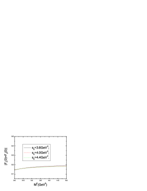
Figure 1: $|F_{1}(0)+F_{2}(0)|$ with the variations of the Borel Parameter $M^{2}$ for EFSR.

Figure 2: $|\frac{[\frac{AA}{CC}]_{s0=20.0GeV^{2}}-[\frac{AA}{CC}]_{s0=4.0GeV^{2}}}{[\frac{AA}{CC}]_{s0=4.0GeV^{2}}}|$ with the variations of the Borel Parameter $M^{2}$ for EFSR.

In the LCSR approach, the uncertainty of the photon light-cone distribution amplitudes, keeping only the lowest-twist few terms of two particles distribution amplitudes, the uncertainty of the condensates, the neglect of the higher dimension condensates, the lack of perturbative QCD corrections, etc, can lead to errors in the predictions. The LCSRs for the form factor $F_{1}(0)+F_{2}(0)$ ( see Eq.(23) and Eq.(25) ) are very sensitive to the values of the parameter $f$, small variations of the $f$ can lead to large changes for the magnetic moment, which is shown in Fig.4. The inclusion of the contributions from the direct instantons may improve the stability of the LCSR, to our knowledge, there exist no such type works on the magnetic moments of the baryon with the LCSR, this may be our next work. In this article, only the nonperturbative interactions of the photons with the $s$ quark line of the form $\langle\gamma(q)|\bar{q}(x)\gamma_{\mu}\gamma_{5}q(0)|0\rangle$ have contributions to the magnetic moment which is different significantly from the corresponding ones with the interpolating current $J(x)$ in Eq.(14), where all the non-local matrix elements $\langle\gamma(q)|\bar{q}(x)\sigma_{\mu\nu}q(0)|0\rangle$, $\langle\gamma(q)|\bar{q}(x)\gamma_{\mu}\gamma_{5}q(0)|0\rangle$, $\langle\gamma(q)|\bar{q}(x)\gamma_{\mu}q(0)|0\rangle$ have contributions to the magnetic moment, and result in more stable sum rules [5]. In the vector dominance model,

$$f\simeq\frac{f_{\rho}m_{\rho}}{g_{\rho}}\simeq 0.028GeV^{2},$$ (26)

with $g_{\rho}=5.5$ and $f_{\rho}=0.2GeV$. To the leading twist accuracy, the light-cone amplitude $\psi(u)$ is a constant which is set to be unity due to the normalization condition.

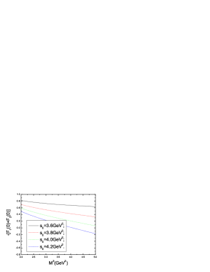
Figure 3: $-[F_{1}(0)+F_{2}(0)]$ with the variations of the Borel Parameter $M^{2}$ for LCSR.

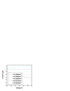
Figure 4: $|F_{1}(0)+F_{2}(0)|$ for different $f$ with the variations of the Borel Parameter $M^{2}$ for LCSR ($s_{0}=3.8GeV^{2}$).

We choose different tensor structures for analysis in different approaches i.e. the EFSR and the LCSR with the same interpolating current $\eta(x)$, the resulting different sum rules always lead to different predictions [5, 15]. The LCSRs with the interpolating current $\eta(x)$ depend heavily on the values of the parameter $f$ and sensitive to the threshold parameter $s_{0}$, the values obtain from the LCSR ( see Eq.(25)) are not as reliable as the corresponding ones from the EFSR ( see Eq.(24)). When the experimental measurement of the magnetic moment of the pentaquark state $\Theta^{+}(1540)$ is possible in the future, we might be able to test the theoretical predictions, select the preferred quark configurations.

Table 1: The values of $\mu_{\Theta^{+}}$ (in unit of $\mu_{N}$)

Reference	$\mu_{\Theta^{+}}$
	$(\mu_{N})$
[5]	0.12 $\pm$ 0.06
[6]	0.08 $\sim$ 0.6
[7]	0.2$\sim$0.3
[8]	0.2$\sim$0.5
[9]	0.08 or 0.23 or 0.19 or 0.37
[10]	0.4
[11]	0.38
[12]	-1.19 or -0.33
[13]	0.71 or 0.56
[14]	0.362
[15]	0.24$\pm$0.02
This Work	-(0.11$\pm$ 0.02)

4 Conclusion

In summary, we have calculated the magnetic moment of the pentaquark state $\Theta^{+}(1540)$ as diquark-diquark-antiquark ($[ud][ud]\bar{s}$) state with both the EFSR and LCSR. We choose different tensor structures for analysis in different approaches (i.e. the EFSR and the LCSR) with the same interpolating current , the resulting different sum rules always lead to different predictions [5, 15]. The EFSRs for the magnetic moment are stable with the variations of the Borel parameter $M^{2}$ and insensitive to the threshold parameter $s_{0}$ (See Fig.1 and Fig.2); the LCSRs in this work depend heavily on the values of the non-local matrix element $\langle\gamma(q)|\bar{q}(x)\gamma_{\mu}\gamma_{5}q(0)|0\rangle$, small variations of the values $f$ can result in large changes about the magnetic moments. The values from the EFSR are more reliable than the corresponding ones from the LCSR. The numerical results from the EFSR are consistent with most of the existing values of theoretical estimations in magnitude, however, with negative sign, $\mu_{\Theta^{+}}=-(0.18\pm 0.03)\frac{e_{\Theta^{+}}}{2m_{\Theta^{+}}}=-(0.11\pm 0.02)\mu_{N}$ . Comparing with Ref.[15], the EFSR with different interpolating currents (standing for different configurations) can lead to very different results for the magnetic moment, although they can both give satisfactory masses for the pentaquark state $\Theta^{+}(1540)$. If the pentaquark state $\Theta^{+}(1540)$ can be interpolated by the linear superposition of both S-type and P-type diquark-diquark-antiquark current $\eta(x)$, the predictions are quantitative and make sense. The magnetic moments of the baryons are fundamental parameters as their masses, which have copious information about the underlying quark structures, different substructures can lead to very different results. The width of the pentaquark state $\Theta^{+}(1540)$ is so narrow, when the small magnetic moment can be extracted from electro- or photo-production experiments eventually in the future, which may be used to distinguish the preferred configurations from various theoretical models, obtain more insight into the relevant degrees of freedom and deepen our understanding about the underlying dynamics that determines the properties of the exotic pentaquark states.

References

- [1] LEPS collaboration, T. Nakano et al , Phys. Rev. Lett. 91 (2003) 012002 ; DIANA Collaboration, V. V. Barmin et al , Phys. Atom. Nucl. 66 (2003) 1715 ; CLAS Collaboration, S. Stepanyan et al. , Phys. Rev. Lett. 91 (2003) 252001; CLAS Collaboration, V. Kubarovsky et al , Phys. Rev. Lett. 92 (2004) 032001; SAPHIR Collaboration, J. Barth et al , Phys. Lett. B572 (2003) 127; A. E. Asratyan, A. G. Dolgolenko and M. A. Kubantsev, Phys. Atom. Nucl. 67 (2004) 682; HERMES Collaboration, A. Airapetian et al , Phys. Lett . B585 (2004) 213; SVD Collaboration, A. Aleev et al , hep-ex/0401024; ZEUS Collaboration, S. V. Chekanov, hep-ex/0404007; CLAS Collaboration, H. G. Juengst, nucl-ex/0312019.
- [2] For example, D. Diakonov, V. Petrov and M. V. Polyakov, Z. Phys. A359 (1997) 305; R. Jaffe and F. Wilczek, Phys. Rev. Lett. 91 (2003) 232003; M. Karliner and H. J. Lipkin, Phys. Lett. B575 (2003) 249; S. L. Zhu, Phys. Rev. Lett. 91 (2003) 232002; J. Sugiyama, T. Doi and M. Oka, Phys. Lett. B581 (2004) 167; M. Eidemüller, Phys. Lett. B597 (2004) 314; T. W. Chiu and T. H. Hsieh, hep-ph/0403020; C. E. Carlson C. D. Carone, H. J. Kwee and V. Nazaryan, Phys. Rev. D70 (2004) 037501; E. Shuryak and I. Zahed, Phys. Lett. B589 (2004) 21; F. Huang, Z. Y. Zhang, Y. W. Yu and B. S. Zou, Phys. Lett. B586 (2004) 69; C. E. Carlson, C. D. Carone, H. J. Kwee and V. Nazaryan, Phys. Lett. B579 (2004)52; Y. S. Oh, H. C. Kim and S. H. Lee , Phys. Rev. D69 (2004) 014009; J. Haidenbauer and G. Krein, Phys. Rev. C68 (2003) 052201; F. Csikor, Z. Fodor, S. D. Katz and T. G. Kovacs, JHEP 0311 (2003) 070; T. D. Cohen, Phys. Lett. B581 (2004) 175; L. Ya. Glozman, Phys. Lett. B575 (2003) 18; N. Ishii, T. Doi, H. Iida, M.Oka, F. Okiharu, H. Suganuma, Phys. Rev. D71 (2005) 034001; N. Mathur, F.X. Lee, A. Alexandru, C. Bennhold, Y. Chen, S. J. Dong, T. Draper, I. Horvath, K. F. Liu, S. Tamhankar and J.B. Zhang, Phys. Rev. D70 (2004) 074508; F. Stancu and D. O. Riska, Phys. Lett. B575 (2003) 242; ; C. E. Carlson C. D. Carone, H. J. Kwee and V. Nazaryan, Phys. Lett. B573 (2003) 101 ; Z. G. Wang, W. M. Yang and S. L. Wan, hep-ph/0504151.
- [3] M. Oka, Prog. Theor. Phys. 112 (2004) 1; S. L. Zhu, Int. J. Mod. Phys. A19 (2004) 3439; S. L. Zhu, hep-ph/0410002; F. E. Close, hep-ph/0311087; B. K. Jennings and K. Maltman, Phys. Rev. D69 (2004) 094020; and references therein.
- [4] A. W. Thomas, K. Hicks and A. Hosaka, Prog. Theor. Phys. 111 (2004) 291.
- [5] P. Z. Huang, W. Z. Deng, X. L. Chen and S. L. Zhu, Phys. Rev. D69 (2004) 074004.
- [6] Q. Zhao, Phys. Rev. D69 (2004) 053009; Erratum-ibid. D70 (2004) 039901.
- [7] H. C. Kim and M. Praszalowicz, Phys. Lett. B585 (2004) 99.
- [8] S. I. Nam, A. Hosaka and H. C. Kim , Phys. Lett. B579 (2004) 43.
- [9] Y. R. Liu, P. Z. Huang, W. Z. Deng, X. L. Chen and S. L. Zhu, Phys. Rev. C69 (2004) 035205.
- [10] T. Inoue, V. E. Lyubovitskij, T. Gutsche and A. Faessler, hep-ph/0408057.
- [11] R. Bijker, M. M. Giannini and E. Santopinto, Phys. Lett. B595 (2004) 260.
- [12] K. Goeke , H. C. Kim , M. Praszalowicz and G. S. Yang , hep-ph/0411195.
- [13] D. K. Hong, Y. J. Sohn and I. Zahed, Phys. Lett. B596 (2004) 191.
- [14] P. Jimenez Delgado , hep-ph/0409128.
- [15] Z. G. Wang, W. M. Yang and S. L. Wan, J. Phys. G31 (2005) 703.
- [16] M. A. Shifman, A. I. Vainshtein and V. I. Zakharov, Nucl. Phys. B147 (1979) 385, 448.
- [17] B. L. Ioffe and A. V. Smilga Nucl. Phys. B232 (1984) 109 ; I. I. Balitsky and A. V. Yung, Phys. Lett. B129 (1983) 328.
- [18] I. I. Balitsky, V. M. Braun and A. V. Kolesnichenko, Sov. J. Nucl. Phys. 44 (1986) 1028 ; Nucl. Phys. B312 (1989) 509; V. L. Chernyak and I. R. Zhitnitsky, Nucl. Phys. B345 (1990) 137 ; V. L. Chernyak and A. R. Zhitnitsky, Phys. Rep. 112 (1984) 173.
- [19] V. M. Braun and I. E. Filyanov, Z. Phys. C44 (1989) 157.
- [20] T. M. Aliev, I. Kanik and M. Savci, Phys. Rev. D68 (2003) 056002 ; T.M. Aliev, A. Ozpineci and M. Savci. Phys. Rev. D66 (2002) 016002 , Erratum-ibid. D67 (2003) 039901; Phys. Rev. D65 (2002) 096004 ; Phys. Rev. D65 (2002) 056008 ; Phys. Lett. B516 (2001) 299 ; Nucl. Phys. A678 (2000) 443 ; T. M. Aliev and A. Ozpineci. Phys. Rev. D62 (2000) 053012.
- [21] R. D. Matheus, F. S. Navarra, M. Nielsen, R. Rodrigues da Silva and S. H. Lee, Phys. Lett. B578 (2004) 323.
- [22] A. De Rujula, H. Georgi and S. L. Glashow, Phys. Rev. D12 (1975) 147 ; T. DeGrand, R. L. Jaffe, K. Johnson and J. E. Kiskis, Phys. Rev. D12 (1975) 2060 ; G. ’t Hooft, Phys. Rev. D14 (1976) 3432 [Erratum-ibid. Phys. Rev. D18 (1978) 2199 ]; E. V. Shuryak, Nucl. Phys. B203 (1982) 93 ; T. Schafer and E. V. Shuryak, Rev. Mod. Phys. 70 (1998) 323 ; E. Shuryak and I. Zahed, Phys. Lett. B 589 (2004) 21.
- [23] M. Eidemuller, F. S. Navarra, M. Nielsen, R. Rodrigues da Silva, hep-ph/0503193.
- [24] M. Aw, M. K. Banerjee, H. Forkel, Phys. Lett. B454 (1999) 147; H. Forkel, hep-ph/0009274.
- [25] V. Chung, H. G. Dosch, M. Kremer, D. Scholl, Nucl. Phys. B197 (1982) 55; H. G. Dosch, M. Jamin and S. Narison, Phys. Lett. B220 (1989) 251.
- [26] Z. G. Wang, W. M. Yang, S. L. Wan, hep-ph/0501015.
- [27] V. M. Belyaev and Y. I. Kogan, Yad. Fiz. 40 (1984) 1035.
- [28] Z. G. Wang, J. Phys. G28 (2002) 3007.
- [29] V. M. Braun and I. E. Filyanov, Z. Phys. C48 (1990) 239; A. Ali and V. M. Braun, Phys. Lett. B359 (1995) 223; G. Eilam, I. Halperin and R. R. Mendel, Phys. Lett. B361 (1995) 137; P. Ball, V. M. Braun and N. Kivel, Nucl. Phys. B649 (2003) 263.
- [30] V. M. Belyaev, V. M. Braun, A. Khodjamirian and R. Rückl, Phys. Rev. D51 (1995) 6177; H. Kim, S. H. Lee and M. Oka, Prog. Theor. Phys. 109 (2003) 371; Z. G. Wang, W. M. Yang and S. L. Wan, Eur. Phys. J. C37 (2004) 223.
- [31] P. Colangelo and A. Khodjamirian, hep-ph/0010175; B. L. Ioffe, hep-ph/0502148.
- [32] R. D. Matheus, S. Narison, hep-ph/0412063.
- [33] W. Wei, P. Z. Huang, H. X. Chen, S. L. Zhu, hep-ph/0503166.