Abstract

A fully numerical method to calculate loop integrals, a numerical contour-integration method, is proposed. Loop integrals can be interpreted as a contour integral in a complex plane for an integrand with multi-poles in the plane. Stable and efficient numerical integrations an along appropriate contour can be performed for tensor integrals as well as for scalar ones appearing in loop calculations of the standard model. Examples of 3- and 4-point diagrams in 1-loop integrals and 2- and 3-point diagrams in 2-loop integrals with arbitrary masses are shown.

Moreover it is shown that numerical evaluations of the Hypergeometric function, which often appears in the loop integrals, can be performed using the numerical contour-integration method.

1 Introduction

In future collider experiments such as at the LHC and ILC, the standard model will be checked with very high precision and a signal of new physics will be searched for through a tiny difference between experimental measurements and theoretical predictions. The theoretical uncertainty must be, at least, one order of magnitude smaller than the experimental one. The theoretical prediction is obtained based on the perturbative calculation of the quantum field theories. The theoretical calculation of a higher order correction with one- or two-loops must be performed in order to meet with experimental requirements. A loop integration is one of the critical issues of a computation of these higher order corrections. Basically there are two methods to perform the loop integration, an analytical method and a numerical one. Though the analytical method gives, in principle, fast and stable results, for many cases it is hard to give a compact expression for the one-loop integral and it is very difficult to perform two-loop computations for the standard model with multiple energy scales.

Numerical methods have also been investigated to perform loop integrals. The symmetrical sampling method was proposed in [1] by Oyanagi et al. in 1988 and has been investigated through a series of papers[2, 3, 4]. Another numerical method, the hybrid method[5], has been proposed. It is to perform a part of the multi-dimensional integrations analytically up to the integrand being a logarithmic form. A remaining integration was performed numerically by Monte Carlo method. Both methods are tuned to calculate up to two-loop/three-point functions with arbitrary masses[6].

Recently another numerical methods using the Sato-Bernstein-Tkachov (SBT) relation is proposed and utilized intensively[10, 11, 12]. A recent review of the method using the SBT relation can be found in [13].

Yet another numerical method has been proposed by de Doncker[14], an ‘$\varepsilon$-algorithm’. This method takes the infinitesimal imaginary parameter appearing in a denominator of the loop integral at finite values, and takes its extrapolation to zero. It is demonstrated that this method can give precise results for a non-scalar one-loop/three-point digram[14].

We propose a new method of loop integrations such as a ‘numerical contour-integration (NCI) method’ in this report. The loop integral can be interpreted as a contour integral in a complex plane for integrands with multi-poles in the plane. We show that the stable and efficient numerical integrations along an appropriate contour for tensor integrals as well as scalar ones appear in loop calculations of the standard model. This method is applicable, so far, up to two-loop/three-point functions with arbitrary masses and arbitrary polynomials of Feynman parameters in the numerator of the integrand. The basic idea of this method and some numerical results are shown in this report.

2 Feynman parameter representation of tensor integrals

The tensor integral of a massless one-loop N-point graph with rank $M\leq N$ in a space-time dimension of $n=4-2\varepsilon$ can be written as,

$$T_{\underbrace{\mu\cdots\nu}_{M}}^{(N)} = \ \int\frac{d^{n}k}{(2\pi)^{n}i}\frac{k_{\mu}\cdots k_{\nu}}{A_{1}A_{2}\cdots A_{N}},$$

where

$$A_{i} = (k+s_{i})^{2}-m^{2}_{i}+i0,$$

$$s_{i} = \sum^{i}_{j=1}p_{j},~{}~{}s_{0}=0,$$

and $p_{i}$ is a four momentum of an $i$’th external particle (incoming), $k_{\mu}$ a loop momentum, and $m_{i}$ the internal masses. An infinitesimal imaginary part ($i0$) is included to obtain analyticity of the integral $T_{\mu\cdots\nu}^{(N)}$. The momentum integration can be done using Feynman’s parameterization which combines the propagators. After the momentum integration, an ultra-violet pole is subtracted under some renormalization scheme. Finally the tensor integral can be expressed using integrals of the type

$$I^{(N)}_{\underbrace{i\cdots k}_{M}} = \int[dx]\frac{x_{i}\cdots x_{k}}{\left(D_{N}-i0\right)^{N-2}},$$ (1)

where

$$\int[dx] = \int^{1}_{0}dx_{1}\int^{1-x_{1}}dx_{2}\cdots\int^{1-\sum^{N-1}_{i=1}x_{i}}dx_{N-1}.$$

An explicit form of the numerator, and a relation between $T_{\mu\cdots\nu}^{(N)}$ and $I^{(N)}_{i\cdots k}$, can be obtained straightforwardly depending on the diagram[15]. The remaining task is to perform the parametric integration of $I^{(N)}_{i\cdots k}$ in Eq.(1), which is called a tensor integral in this report. (When the numerator of the integrand is unity, it is called a scalar integral.)

3 one-loop/three-point

A general formula of the tensor integral for the one-loop/three-point function with arbitrary masses is[1]

$$I^{(3)} = \int_{0}^{1}dx\int_{0}^{1-x}dy\frac{f(x,y)}{D_{3}-i0},$$

$$D_{3} = (M_{1}x-M_{2}y)^{2}-rxy+m_{31}^{2}x+m_{32}^{2}y+m_{2}^{2},$$

where

$$r = s-(M_{1}+M_{2})^{2},$$

$$m_{31}^{2} = -M_{1}^{2}+m_{1}^{2}-m_{2}^{2},$$

$$m_{32}^{2} = -M_{2}^{2}+m_{3}^{2}-m_{2}^{2},$$

$$M_{1}^{2} = p_{1}^{2},$$

$$M_{2}^{2} = p_{2}^{2},$$

$$s = (p_{1}+p_{2})^{2}.$$

Figure 1: 1-loop/3-point diagram

A numerator of the integrand, $f(x,y)$, can be any polynomial of Feynman parameters $x$ and $y$ with rank $M\leq 3$. Momentum and mass assignments are shown in Figure 1.

The integration region is a 2-dimensional simplex with three sides. Those sides are

$$L_{x} = \{(x,y)|0\leq x\leq 1,y=0\},$$

$$L_{y} = \{(x,y)|x=0,0\leq y\leq 1\},$$

$$L_{xy} = \{(x,y)|y=1-x,0\leq x\leq 1\}.$$

Singular points (second pole) of the integrand form a parabola (or hyperbola), which is

$${\cal P} = \{(x,y)|D_{3}=0\}.$$

The focal point of the parabola is on the opposite side of the origin with respect to the parabola line. When one integration-variable is fixed, the remaining one-parameter integration may intersect a pole on the line ${\cal P}$. This integration can be done numerically as a contour integral along an appropriate contour with correct analyticity. For a stable integration, it must be avoided that the contour intersects more than one pole, or that a pole is at the end point of the contour. These requirements are satisfied by taking an appropriate coordinate system instead of a simple $(x,y)$ coordinate of Feynman parameters. Basically we take polar-coordinates with an origin on the side $L_{xy}$. Coordinate systems we used are categorized by the following cases;

1. ${\cal N}[(L_{x}\cup L_{y}\cup L_{xy})\cap{\cal P}]=0$:
   ${\cal N}[{\cal A}]$ are number of elements of a set ${\cal A}$. There is no singular points in the integration region. The origin is set at the nearest point to the line ${\cal P}$ on the side $L_{xy}$.

2. ${\cal N}[L_{xy}\cap{\cal P}]=1$ $\wedge$ ${\cal N}[(L_{x}\cup L_{y})\cap{\cal P}]=0$:
   The origin of the coordinate system is set at a point such as $\{L_{xy}\cap{\cal P}\}$. Though a pole is at the origin, the singularity is canceled out against the Jacobian on the numerator, i.e. the measure at the origin is zero in the polar-coordinates. Then the integration is free from singularities.

3. ${\cal N}[L_{xy}\cap{\cal P}]=2$ $\wedge$ ${\cal N}[(L_{x}\cup L_{y})\cap{\cal P}]=0$:
   The origin is set at the center of two elements of $\{L_{xy}\cap{\cal P}\}$. Then the contour along $r$ intersects the line ${\cal P}$ only once for any value of $\phi$. We can take an appropriate contour avoiding the pole with correct analyticity.

4. ${\cal N}[L_{xy}\cap{\cal P}]=2$ $\wedge$ ${\cal N}[L_{x}\cap{\cal P}]=2$ $\wedge$ ${\cal N}[L_{y}\cap{\cal P}]=2$:
   The integration region is divided into three regions by two lines, one connects between centers of two elements of $L_{xy}\cap{\cal P}$ and those of $L_{x}\cap{\cal P}$, the other connects between centers of two elements of $L_{xy}\cap{\cal P}$ and $L_{y}\cap{\cal P}$. The origins of the coordinate frames are set at the three corner of the simplex, $(0,0)$, $(1,0)$ and $(0,1)$. In each region, the contour along $r$ intersects the line ${\cal P}$ only once for any value of $\phi$. We can take an appropriate contour avoiding the pole with correct analyticity.

Numerical integrations are performed based on the ‘Good Lattice Point (GLP) Method[16]’, which uses a deterministic series of numbers. For smooth functions it shows very efficient convergence compared with a Monte Carlo integration based on random sampling. Moreover both imaginary and real parts can be integrated simultaneously.

Here we show several examples of one-loop/three-point functions.

• Case 1:$m_{1}=m_{3}=M_{1}=M_{2}=150$ GeV, $m_{2}=91$ GeV, $f(x,y)=1$.

  Table 1 $\sqrt{s}$ real/imag. analytic[17] NCI result error calls 310 real $0.1110\times 10^{-3}$ $0.110975\times 10^{-3}$ $0.23\times 10^{-10}$ 350 imag. $0.7162\times 10^{-4}$ $0.716174\times 10^{-4}$ 500 real $0.2285\times 10^{-5}$ $0.228498\times 10^{-5}$ $0.39\times 10^{-10}$ 350 imag. $0.4731\times 10^{-4}$ $0.473072\times 10^{-4}$ 1000 real $-0.6103\times 10^{-5}$ $-0.610293\times 10^{-5}$ $0.22\times 10^{-11}$ 582 imag. $0.1551\times 10^{-4}$ $0.155066\times 10^{-4}$

  This is an infrared-divergence free integral with only heavy particles involved. Very good agreements can be obtained between analytical results (formulae given in ref.[17]) and the NCI method as shown in the above table with only several hundred sampling points.

• Case 2:$m_{1}=m_{3}=M_{1}=M_{2}=m_{e}$, $\sqrt{s}=1000$ GeV, $f(x,y)=1$.

  Table 2 $m_{2}(GeV)$ real/imag. analytic[17] NCI results error calls $10^{-5}$ real $-0.641175\times 10^{-3}$ $-0.641175\times 10^{-3}$ $0.20\times 10^{-9}$ 6732 imag. $~{}0.115741\times 10^{-3}$ $~{}0.115740\times 10^{-3}$ $10^{-7}$ real $-0.907973\times 10^{-3}$ $-0.907973\times 10^{-3}$ $0.22\times 10^{-7}$ 6732 imag. $~{}0.144676\times 10^{-3}$ $~{}0.144674\times 10^{-3}$ $10^{-9}$ real $-0.117483\times 10^{-2}$ $-0.117479\times 10^{-2}$ $0.10\times 10^{-6}$ 28621 imag. $~{}0.173611\times 10^{-3}$ $~{}0.173618\times 10^{-3}$

  This is an infrared-divergent case with a fictitious photon mass of $10^{-5}$ to $10^{-9}$ GeV. Very good agreements can be obtained between analytical results and the NCI, even for the infrared-divergent case with several thousand sampling points.

• Case 3:$m_{1}=m_{3}=80$ GeV, $M_{1}=M_{2}=170$ GeV, $M_{2}=5$ GeV, $\sqrt{s}=357$ GeV
  

  Table 3 $f(x,y)$ real/imag. $FF\cite[cite]{[\@@bibref{}{ff}{}{}]}$ NCI results error calls $1$ real $-0.623169\times 10^{-4}$ $-0.623169\times 10^{-4}$ $0.18\times 10^{-14}$ 1567 imag. $~{}0.132340\times 10^{-4}$ $~{}0.132340\times 10^{-4}$ $x$ real $-0.171520\times 10^{-4}$ $-0.171520\times 10^{-4}$ $0.43\times 10^{-9}$ 1567 imag. $~{}0.579780\times 10^{-5}$ $~{}0.579780\times 10^{-5}$ $x^{2}$ real $-0.859550\times 10^{-5}$ $-0.859550\times 10^{-5}$ $0.13\times 10^{-9}$ 1567 imag. $~{}0.487062\times 10^{-5}$ $~{}0.487063\times 10^{-5}$ $x\times y$ real $-0.324021\times 10^{-5}$ $-0.324021\times 10^{-5}$ $0.11\times 10^{-9}$ 1567 imag. $~{}0.296541\times 10^{-6}$ $~{}0.296540\times 10^{-6}$

The tensor integration can be done as well as the scalar one as shown in Table 3. NCI results show a very good agreement with those from the $FF$ package[18] developed by van Oldenborgh.

4 one-loop/four-point

A general formula for the one-loop/four-point function with arbitrary masses is[3]

$$I^{(4)} = \int_{0}^{1}dz\int_{0}^{1-z}dy\int_{0}^{1-y-z}dx\frac{f(x,y,z)}{D_{4}-i0},$$

$$D_{4} = (M_{1}x-M_{2}y)^{2}-rxy+m_{41}^{2}x+m_{42}^{2}y+m_{43}^{2},$$

where

$$t = (p_{2}+p_{3})^{2},$$

$$u = (p_{1}+p_{3})^{2},$$

$$m_{41}^{2} = -M_{1}^{2}+m_{1}^{2}-m_{2}^{2}-z(s+u-2M_{1}^{2}-M_{2}^{2}-M_{3}^{2}),$$

$$m_{42}^{2} = -M_{2}^{2}+m_{3}^{2}-z(t+M_{2}^{2}-M_{3}^{2}),$$

$$m_{43}^{2} = m_{2}^{2}+(-M_{3}^{2}+m_{4}^{2}-m_{2}^{2})z+tz^{2}$$

A numerator of the integrand, $f(x,y,z)$, can be any polynomial of Feynman parameters, $x$, $y$ and $z$ with rank $M\leq 4$. Momentum and mass assignments are shown in Figure 2.

Figure 2: 1-loop/4-point diagram

The integration region is a 3-dimensional simplex. In order to perform the contour integral very efficiently in this three-dimensional integration-parameter space, we have introduced a new coordinate system as shown in Figure 3, named ‘Wedge coordinate system’.

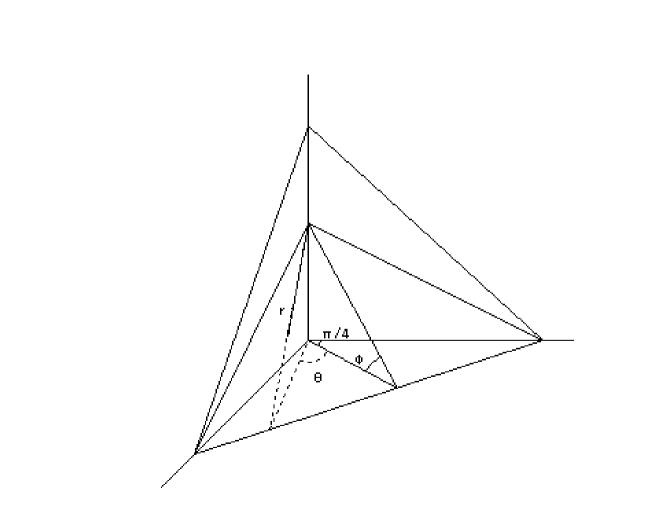
Figure 3: Parametrization of the wedge coordinate

A relation between an usual Cartesian coordinate system and the wedge coordinate system is given as

$$x = r\cos{\phi^{\prime}}\sin{\left(\theta+\frac{\pi}{4}\right)},$$

$$y = r\cos{\phi^{\prime}}\cos{\left(\theta+\frac{\pi}{4}\right)},$$

$$z = (r_{max}-r)\sin{\phi^{\prime}},$$

where

$$\tan{\phi^{\prime}} = \cos{\theta}\tan{\phi},$$

$$r_{max} = \sqrt{\frac{\tan^{2}{\phi}}{2}+\frac{1}{2\cos^{2}{\theta}}}.$$

The Feynman parameter integration now becomes

$$I^{(4)} = \int_{0}^{1}dz\int_{0}^{1-z}dy\int_{0}^{1-y}dx\frac{f(x,y,z)}{D_{4}-i0}$$

$$= \int_{0}^{r_{max}}dr\int_{-\pi/4}^{\pi/4}d\theta\int_{0}^{\tan^{-1}{\sqrt{2}}}d\phi~{}~{}r(r_{max}-r)\frac{\cos{\theta}\cos^{3}{\phi^{\prime}}}{\cos^{2}{\phi}}\frac{f(r,\theta,\phi)}{D_{4}-i0}.$$

When $\phi$ is fixed, the remaining integration region is a triangle. The intersection between this triangle and a hyper-surface which satisfies $D_{4}=0$ is a parabola (or hyperbola) similar to the one-loop/three-point case. The variable $r$ is extended into the complex plane. When both $\phi$ and $\theta$ are fixed, we can take an appropriate contour for $r$ which crosses a pole only once for any $\phi$ and $\theta$.

Here we show several examples of one-loop/four-point functions.

• Case 1:$e^{+}e^{-}\rightarrow W^{+}W^{-}$.
  $m_{1}=m_{3}=80$ GeV, $m_{2}=0$, $m_{4}=91$ GeV, $M_{1}=M_{2}=m_{e}$, $M_{3}=M_{4}=80$ GeV, $\sqrt{s}=500$ GeV, $\theta=\angle(P_{1},P_{4})$.

  Table 4 $\cos{\theta}$ real/imag. $FF\cite[cite]{[\@@bibref{}{ff}{}{}]}$ NCI results error calls $-0.5$ real $-0.459774\times 10^{-9}$ $-0.459774\times 10^{-9}$ $0.67\times 10^{-13}$ 1567 imag. $0.711583\times 10^{-9}$ $0.711582\times 10^{-9}$ $0.0$ real $-0.588538\times 10^{-9}$ $-0.588539\times 10^{-9}$ $0.10\times 10^{-12}$ 1567 imag. $0.962985\times 10^{-9}$ $0.962985\times 10^{-9}$ $0.5$ real $-0.849170\times 10^{-9}$ $-0.849167\times 10^{-9}$ $0.10\times 10^{-13}$ 2553 imag. $0.155695\times 10^{-8}$ $0.155695\times 10^{-8}$

  Though a massless particle (neutrino) appears in the loop in this case, this is infrared-divergence free. The NCI with several thousand sampling points gives very good agreement with $FF$.

• Case 2:$e^{+}e^{-}\rightarrow zz$.
  $m_{1}=m_{3}=m_{4}=m_{e}$, $m_{2}=91$ GeV, $M_{1}=M_{2}=m_{e}$, $M_{3}=M_{4}=91$ GeV, $\sqrt{s}=500$ GeV, $\theta=\angle(P_{1},P_{4})$.

  Table 5 $\cos{\theta}$ real/imag. $FF\cite[cite]{[\@@bibref{}{ff}{}{}]}$ NCI results error calls $-0.5$ real $-0.89532\times 10^{-9}$ $-0.89540\times 10^{-9}$ $0.54\times 10^{-12}$ $2M$ imag. $-0.23060\times 10^{-9}$ $-0.23049\times 10^{-9}$ $0.0$ real $-0.11548\times 10^{-8}$ $-0.11549\times 10^{-8}$ $0.78\times 10^{-11}$ $2M$ imag. $-0.33447\times 10^{-9}$ $-0.33433\times 10^{-9}$ $0.5$ real $-0.17129\times 10^{-8}$ $-0.17134\times 10^{-8}$ $0.96\times 10^{-11}$ $2M$ imag. $0.60873\times 10^{-9}$ $0.60862\times 10^{-9}$

  A light particle (an electron) exists in the loop in this case. Although it requires high statistics of about two million sampling points even by the GLP, the result shows good agreement with $FF$.

Though only scalar integrations are shown here, tensor integrations with an arbitrary polynomial in the numerator can be done as well.

5 two-loop/two-point

A general formula of the two-loop/two-point function with arbitrary masses is[4]

$$I^{(2)} = \int_{0}^{1}dx_{1}dx_{2}dx_{3}dx_{4}dx_{5}\delta\left(1-\sum_{i=1}^{5}x_{i}\right)\frac{f(x_{i})}{DC-i0},$$

where

$$D = -p^{2}\left(x_{5}\left(x_{1}+x_{3}\right)\left(x_{2}+x_{4}\right)+\left(x_{1}+x_{2}\right)x_{3}x_{4}+\left(x_{3}+x_{4}\right)x_{1}x_{2}\right)+C{\bar{M}}^{2},$$

$$C = \left(x_{1}+x_{2}+x_{3}+x_{4}\right)x_{5}+\left(x_{1}+x_{2}\right)\left(x_{3}+x_{4}\right),$$

$${\bar{M}}^{2} = \sum_{i=1}^{5}x_{i}m_{i}^{2},$$

and $m_{i}$ are the internal masses. A particle number assignment is shown in Figure 4. Here $f(x_{i})$ is any polynomial of Feynman parameters $x_{i}$ with rank $M\leq 2$.

Figure 4: 2-loop/2-point diagram

Feynman parameter integration with four independent variables must be performed after $x_{5}$ integration eliminates a delta-function. It is very hard to make any intuitive optimization for the integration because four-dimensional space is beyond our imagination. We simply employ the following coordinate system: At first one-point on the edge-simplex of $x_{1}+x_{2}+x_{3}+x_{4}=1$ is chosen. Then take a variable $r$ as a distance between a origin of the coordinate ($x_{1}=x_{2}=x_{3}=x_{4}=0$) and the point on a straight line from the origin to the point in the edge-simplex. This $r$ is extended into the complex plane and chosen to follow an appropriate contour to avoid singularities. Here we show two examples of two-loop/two-point functions.

• Case 1:$m_{1}=m_{2}=m_{3}=m_{4}=m_{0}=150$ GeV and $m_{5}=91.17$ GeV.

  Table 6
  $p^{2}/m_{0}^{2}$ real/imag. Kreimer[20] NCI results 2.0 real 2.664 2.6647(2) 4.0 real 25.85 25.87(2) 4.1 real 21.506 21.47(3) imag. 12.16 12.15(3) 4.3 real 15.246 15.19(3) imag. 17.013 17.29(3) 5.0 real 3.668 3.63(4) imag. 19.503 19.48(4) 7.0 real -6.7939 -6.78(4) imag. 13.918 13.89(4) 10.0 real -8.793 -8.792(1) imag. 8.865 8.846(1)

  In this case, integrations are done by Monte Carlo method using BASES[19]. NCI results show good agreement with the analytical results by Kreimer[20], within the statistical error of the Monte Carlo integration.

• Case 2:$m_{1}=1$ GeV, $m_{2}=2$ GeV, $m_{3}=4$ GeV, $m_{4}=5$ GeV, $m_{5}=3$ GeV.

  Table 7 $p^{2}(GeV^{2})$ real/imag. Bauberger et al.[21] NCI results 0.1 real -0.287238(3) -0.287240(6) 0.5 real -0.294592(3) -0.294594(6) 1.0 real -0.304521(3) -0.304523(6) 5.0 real -0.452520(3) -0.452527(9) 10.0 real -0.488153(2) -0.48807(5) imag. -0.353217(2) -0.35307(4) 50.0 real 0.173901(2) 0.17397(2) imag. -0.118080(2) -0.11805(2)

This is an example with a very simple mass assignment. The result of the NCI method is compared with that from the analytical calculation obtained by Bauberger and Böhm[21], and gives also very good agreement. The same example is treated using the SBT relation by Passarino and Uccirati[11] with very good agreement too.

Though only scalar integrations are shown here, tensor integrations with an arbitrary polynomial in the numerator can be done as well.

6 two-loop/three-point

Figure 5: 2-loop vertex diagram (non-planer type)

A general formula of the two-loop/three-point function (non-planar configuration) with arbitrary masses can be expressed as

$$I^{(3)} = \frac{1}{8}\int_{0}^{1}dz_{1}dz_{2}dz_{3}\delta\left(1-\sigma z\right)z_{1}z_{2}z_{3}\int_{-1}^{1}dy_{1}dy_{2}dy_{3}\frac{f(y_{i},z_{j})}{\left(D_{3}-i0\right)^{2}},$$

after some transformation of the original Feynman parametrization[6]. Here the denominator is

$$D_{3} = {}^{t}{\overrightarrow{y}}A{\overrightarrow{y}}+^{t}{\overrightarrow{b}}\cdot{\overrightarrow{y}}+c,$$

where

$${\overrightarrow{y}} = \left(\begin{array}[]{c}y_{1}\\ y_{2}\\ y_{3}\end{array}\right),$$

$$A = \frac{1}{4}\left(\begin{array}[]{ccc}-z_{1}^{2}(z_{2}+z_{3})s_{1}&z_{1}z_{2}z_{3}(-s_{1}-s_{2}+s_{3})/2&z_{1}z_{2}z_{3}(-s_{1}+s_{2}-s_{3})/2\\ z_{1}z_{2}z_{3}(-s_{1}-s_{2}+s_{3})/2&-z_{2}^{2}(z_{3}+z_{1})s_{2}&z_{1}z_{2}z_{3}(+s_{1}-s_{2}-s_{3})/2\\ z_{1}z_{2}z_{3}(-s_{1}+s_{2}-s_{3})/2&z_{1}z_{2}z_{3}(+s_{1}-s_{2}-s_{3})/2&-z_{3}^{2}(z_{1}+z_{2})s_{3}\end{array}\right),$$

$${\overrightarrow{b}} = \frac{1}{2}U\left(\begin{array}[]{c}z_{1}(m_{3}^{2}-m_{4}^{2})\\ z_{2}(m_{5}^{2}-m_{6}^{2})\\ z_{3}(m_{2}^{2}-m_{1}^{2})\end{array}\right),$$

$$c = \frac{1}{4}U\left[z_{1}s_{1}+z_{2}s_{2}+z_{3}s_{3}-2(m_{3}^{2}+m_{4}^{2})z_{1}-2(m_{5}^{2}+m_{6}^{2})z_{2}-2(m_{1}^{2}+m_{2}^{2})z_{3}\right],$$

$$U = z_{1}z_{2}+z_{2}z_{3}+z_{3}z_{1},$$

and $s_{i}=p_{i}^{2}$, and $m_{i}$ are the internal masses. Here ${}^{t}{\overrightarrow{v}}$ gives a transposed vector of ${\overrightarrow{v}}$. For the $y$ integration, we employ the SBT relation as

$$\frac{1}{D_{3}^{2}} = \frac{1}{\beta}\left[1+\frac{1}{2}~{}^{t}\left({\overrightarrow{y}}-{\overrightarrow{\eta}}\right)\cdot{\overrightarrow{\partial}_{y}}\right]\frac{1}{D_{3}},$$

$$\beta = c-\left({}^{t}{\overrightarrow{b}}A^{-1}{\overrightarrow{b}}\right),$$

$${\overrightarrow{\eta}} = -A^{-1}{\overrightarrow{b}}$$

$${\overrightarrow{\partial}_{y}} = \left(\frac{\partial~{}~{}}{\partial y_{1}},\frac{\partial~{}~{}}{\partial y_{2}},\frac{\partial~{}~{}}{\partial y_{3}}\right).$$

The $y_{i}$ are left as real variables. In order to avoid singularities in $\beta^{-1}$ and $D_{3}^{-1}$, the $z_{i}$ are extended into the complex plane. After the $z_{3}$ integration to eliminate the $\delta$-function, the polar coordinates, $z_{1}=r_{z}\sin\theta_{z},~{}z_{2}=r_{z}\cos\theta_{z}$ are introduced. This $r_{z}$ is extended into the complex plane and chosen along an appropriate contour to avoid singularities. Here we show one example of a two-loop/three-point function.

• $m_{1}=m_{2}=m_{4}=m_{5}=150$ GeV, $m_{3}=m_{6}=91.17$ GeV, and $s1=s2=150^{2}~{}{\rm GeV}^{2}$.

  Table 8

  $s_{3}/m_{1}^{2}$	Fujimoto et al.[6]	NCI results
  4.5	$2.09(2)\times 10^{-9}$	$2.049(2)\times 10^{-9}$
  5	$1.43(1)\times 10^{-9}$	$1.464(2)\times 10^{-9}$
  12	$-8.37(3)\times 10^{-10}$	$-8.24(4)\times 10^{-10}$
  20	$-5.61(3)\times 10^{-10}$	$-5.60(1)\times 10^{-10}$

The Monte Carlo integration package, BASES, is used for the numerical integration. The results agree well with those in refs.[6, 22]

Though only scalar integrations are shown here, tensor integrations with arbitrary polynomial in the numerator can be done as well.

7 Numerical evaluations of the Hypergeometric functions

So far we discussed in previous sections loop-integrals in the standard model with arbitrary masses. In this section we would like to treat a massless theory such as QCD. A general one-loop/four-point function in a massless theory can be expressed by the following tensor integrals:

$$I^{(4)}(s,t;n_{x},n_{y},n_{z}) = \left(4\pi\mu^{2}\right)^{-\varepsilon_{IR}}\int_{0}^{1}dx~{}dy~{}dz\frac{x^{n_{x}}y^{n_{y}}z^{n_{z}}}{(D_{4}-i0)^{2-\varepsilon_{IR}}},$$

$$D_{4} = -xzs-y(1-x-y-z)t,$$

where $s=(p_{1}+p_{2})^{2}$, and $t=(p_{1}+p_{4})^{2}$. Here we set all particles massless. In order to cure an infrared divergence, the space-time dimension is set to be $n=4+2\varepsilon_{IR}$ after the $\overline{MS}$ renormalization. The tensor integration can be done analytically and be represented by a finite number of terms with Beta and Hypergeometric functions as[23];

$$I^{(4)}(s,t;n_{x},n_{y},n_{z})=\frac{1}{s~{}t}\frac{B(n_{x}+\varepsilon_{IR},n_{y}+n_{z}+\varepsilon_{IR})}{1-\varepsilon_{IR}}$$

$$\times \biggl{[}\left(\frac{-{\tilde{t}}}{4\pi\mu^{2}}\right)^{\varepsilon_{IR}}\left(\frac{-t}{s}\right)^{n_{x}}\frac{n_{x}}{\prod_{j=1}^{n_{x}}({n_{x}}-j+\varepsilon_{IR})}B(1+n_{z},n_{x}+n_{y}+\varepsilon_{IR})$$

$$\times {{}_{2}F_{1}}\left(1+n_{x},n_{x}+n_{z}+\varepsilon_{IR},1+n_{x}+n_{y}+n_{z}+\varepsilon_{IR},-\frac{{\tilde{u}}}{{\tilde{s}}}\right)$$

$$+ \left(\frac{-{\tilde{s}}}{4\pi\mu^{2}}\right)^{\varepsilon_{IR}}\sum_{l=0}^{n_{x}}\left(\frac{-s}{t}\right)^{l}\frac{\prod_{j=1}^{l}(l-j-n_{x})}{\prod_{j=1}^{l}(l-j+\varepsilon_{IR})}B(1+n_{y},l+n_{z}+\varepsilon_{IR})$$

$$\times {{}_{2}F_{1}}\left(1+l,l+n_{z}+\varepsilon_{IR},1+l+n_{y}+n_{z}+\varepsilon_{IR},-\frac{{\tilde{u}}}{\bar{t}}\right)\biggr{]},$$

$${{\tilde{s}}} = s+i0,$$

$${{\tilde{t}}} = t+i0,$$

$${\bar{t}} = t-i0,$$

$${{\tilde{u}}} = u+i0=(p_{1}+p_{3})^{2}+i0.$$

For the infrared-finite case, evaluation of the loop integral can be done if we can perform the numerical calculation of the Hypergeometric function of a type

$${{}_{2}F_{1}}\left(1+l,l+m,1+l+m+n,z\right) = \frac{\Gamma(1+l+m+n)}{\Gamma(l+m)\Gamma(1+n)}\int_{0}^{1}d\tau\frac{\tau^{l+m-1}(1-\tau)^{n}}{(1-z\tau)^{1+l}}$$

where $l,m,n>0$ are integer numbers and $z$ a complex variable. This integration can be performed easily using the NCI.

$l$	$m$	$n$	real/imag.	$Mathematica\cite[cite]{[\@@bibref{}{mathematica}{}{}]}$	NCI	calls
1	1	1	real	$-0.1453322029\times 10^{-1}$	$-0.1453322029\times 10^{-1}$	4149
			imag.	$-0.1507964474\times 10^{0~{}~{}}$	$-0.1507964474\times 10^{0~{}~{}}$
1	2	3	real	$0.8417767168\times 10^{-1}$	$0.8417767169\times 10^{-1}$	4149
			imag.	$-0.2290221044\times 10^{0~{}~{}}$	$-0.2290221044\times 10^{0~{}~{}}$
2	1	1	real	$0.1087664688\times 10^{-1}$	$0.1087664688\times 10^{-1}$	4149
			imag.	$0.2638937829\times 10^{-1}$	$0.2638937829\times 10^{-1}$
2	3	4	real	$-0.2890568082\times 10^{-1}$	$-0.2890568082\times 10^{-1}$	6732
			imag.	$0.5578978464\times 10^{-1}$	$0.5578978464\times 10^{-1}$
3	1	2	real	$-0.1026721798\times 10^{-1}$	$-0.1026721798\times 10^{-1}$	6732
			imag.	$-0.5654866776\times 10^{-2}$	$-0.5654866776\times 10^{-2}$
3	4	5	real	$0.8121358824\times 10^{-2}$	$0.8121358824\times 10^{-2}$	6732
			imag.	$-0.1274636264\times 10^{-1}$	$-0.1274636264\times 10^{-1}$

Table 9 numerical calculation of the Hypergeometric function at $z=10$.

The results from the NCI method with the GLP numerical integration at $z=10+i0$ are shown in Table 9 comparing them with those obtained by $Mathematica$[24]. The ten-digit agreement with $Mathematica$ can be obtained with only four to seven thousand sampling points in the GLP.

8 Summary

We have developed a fully numerical method, named ‘numerical contour integration (NCI)’ method, to calculate loop integrals. Loop integrals can be interpreted as a contour integral in a complex plane for an integrand with multi-poles in the plane. For the one-loop/three-point case with arbitrary masses in the standard model, both scalar and tensor integrals have been obtained by the NCI method with five to seven digits accuracy. For the one-loop/four point case, scalar integrals have been calculated with about 0.1% accuracy. For the above two cases, the ‘Good Lattice Point’ method is used for the numerical integration. Those results are compared with analytical calculation or $FF$ and show a very good agreement. The NCI method has been applied also to two-loop integrals. For two- and three-point integrals at the two-loop level, it is demonstrated that the NCI method can give numerical results of the loop integrals with good accuracy using the Monte Carlo integration package BASES. Those results show a good agreement with previous calculations. The extension to the general tensor cases is straight forward, since the NCI is a purely numerical method. Moreover it is shown that the numerical evaluation of the Hypergeometric function, which appears in the one-loop/four-point tensor-integrals in massless QCD, has been performed with ten-digit accuracy using the GLP method.

Authors would like to thank Drs. J. Fujimoto, T. Ishikawa and Y. Shimizu for continuous discussions on this subject and their useful suggestions. We are grateful to Prof. J. Vermaseren for his proofreading the manuscript which improved the English very much.

This work was supported in part by the Ministry of Education, Science and Culture under the Grant-in-Aid No. 11206203 and 14340081.

References

• [1] Y. Oyanagi, T. Kaneko, T. Sasaki, S. Kawabata, Y. Shimizu, “How to Calculate One-Loop Diagram”, in ‘Perspective of Particle Physics’, ed. S. Matsuda et al., World Scientific (1988) p.369, KEK-Preprint 88-6.
• [2] J. Fujimoto, Y. Shimizu, K. Kato, Y. Oyanagi, “Numerical Approach to One-loop Integrals”, in ‘Proc. of the International Conference on Computing in High Energy Physics ’91’, ed. Y. Watase and F. Abe, Universal Academy Press inc., (1991) p407,
• [3] J. Fujimoto, Y. Shimizu, K. Kato, Y. Oyanagi, Prog. Theor. Phys. 87 (1992),1233.
• [4] J. Fujimoto, Y. Shimizu, K. Kato, Y. Oyanagi, ”Numerical Approach to loop Integrals”, in ‘New Computing Techniques in Physics Research II’, ed. D. Perret-Gallix, World Scientific, (1992) p625.
• [5] J. Fujimoto, Y. Shimizu, K. Kato, Y. Oyanagi, “Numerical Approach to Two-loop Integrals”, KEK-Preprint 92-213.
• [6] J. Fujimoto, Y. Shimizu, K. Kato, T. Kaneko, Int. Journ. of Mod. Phys. C6 (1995) 525.
• [7] M. Sato, “Theory of prehomogeneous vector spaces (Algebraic part)” (The English translation of Sato’s lecture from Shintani’s Note(1970)), Nagoya Math. J. 120 (1990),1.
• [8] L.N. Bernstein, Functional Analysis and its Applications 6 (1972) 66.
• [9] F.V. Tkachov, Nucl. Instrum. Methods A389 (1997) 309.
• [10] G. Passarino, Nucl. Phys. B629 (2001) 257,
A. Ferroglia, M. Passera, G. Passarino, S. Uccirati, Nucl. Phys. B650 (2003) 162; ibid., B680 (2004) 199.
• [11] G. Passarino, S. Uccirati, Nucl. Phys. B629 (2002) 97.
• [12] M.M. Weber, Acta Phys. Polonica B55 (2004) 2655.
• [13] S. Uccirati, Acta Phys. Polonica B55 (2004) 2573.
• [14] E. de Doncker, Y. Shimizu, J. Fujimoto, F. Yuasa, K. Kaugars, L. Cucos, J. Van Voorst, Nucl. Instrum. Methods A534 (2004) 269.
• [15] See section 5 in G. Bélanger, F. Boudjema, J. Fujimoto, T. Ishikawa, T. Kaneko, K. Kato, Y. Shimizu, hep-ph/0308080.
• [16] For example, see I.H. Sloan, S. Joe, “Lattice Methods for Multiple Integration”, Oxford Univ. Press, Oxford, 1994.
• [17] J. Fujimoto, M. Igarashi, N. Nakazawa, Y. Shimizu, K. Tobimatsu, Suppl. Prog. Theor. Phys. 100 (1990) 1.
• [18] G.J. van Oldenborgh, Compute. Phys. Commun. 58 (1991) 1.
• [19] S. Kawabata, Comp. Phys. Commun. 41 (1986) 127; ibid., 88 (1995) 309.
• [20] Numbers are obtained though a private communication with D. Kreimer. His calculation is performed based on the method described in D. Kreimer, Phys. Lett. B273 (1991) 277.
• [21] S. Bauberger, M. Böhm, Nucl. Phys. B445 (1995) 25.
• [22] D. Kreimer, Phys. Lett. B292 (1992) 341,
A. Frink, U. Kilian, D. Kreimer, Nucl. Phys. B488 (1997) 426.
• [23] Y. Kurihara, J. Fujimoto, T. Ishikawa, K. Kato, S. Kawabata, T. Munehisa, H. Tanaka, Nucl. Phys. B654 (2003) 301.
• [24] $Mathematica$ ver.5.0, Wolfram Reserach, Inc.