Abstract

The dynamics of five dimensional Wilson line phases at finite temperature is studied in the one-loop approximation. We show that at temperatures of order $T\sim 1/L$, where $L$ is the length of the compact space, the gauge symmetry is always restored and the electroweak phase transition appears to be of first order.

Particular attention is devoted to the study of a recently proposed five dimensional orbifold model (on $S^{1}/{\bf Z}_{2}$) where the Wilson line phase is identified with the Higgs field (gauge-Higgs unification). Interestingly enough, an estimate of the leading higher-loop “daisy” (or “ring”) diagram contributions to the effective potential in a simple five dimensional model, seems to suggest that the electroweak phase transition can be studied in perturbation theory even for Higgs masses above the current experimental limit of 114 GeV. The transition is still of first order for such values of the Higgs mass. If large localized gauge kinetic terms are present, the transition might be strong enough to give baryogenesis at the electroweak transition.

1 Introduction

Theories in extra dimensions are interesting alternatives to more standard four-dimensional (4D) extensions of the Standard Model (SM). In particular, there has recently been a lot of interest in theories with compact extra dimensions at the TeV scale [2]. On the theoretical side they are, among other things, a possible framework to solve the gauge hierarchy problem and, from a more phenomenological point of view, they would potentially be tested at the Large Hadron Collider (LHC).

A particularly interesting scenario provided by theories in extra dimensions is the possibility of identifying the Higgs field with the internal component of a gauge field [3]. Several models of this sort have recently been considered, with [4] or without [5, 6] supersymmetry, in various set-ups. Models invoking this scenario, given the origin of the Higgs field, are sometimes called models with gauge-Higgs unification. Electroweak symmetry breaking occurs radiatively in these theories, and is equivalent to a Wilson line symmetry breaking [7, 8, 9], since the vacuum expectation value (VEV) of the Higgs field is proportional to the value of the Wilson line phase. In minimal 5D non-supersymmetric single-Higgs models, the Higgs potential is entirely radiatively generated and non-local in the extra dimensions. The models are highly predictive and the gauge hierarchy problem is solved. Matter can also be introduced in this set-up, with the possibility of naturally having a hierarchy of fermion masses [6]. Although some problems have still to be solved before getting a completely realistic model, theories with gauge-Higgs unification are definitely an interesting framework for physics beyond the SM.

Aim of the present paper is to study in some detail the dynamics of 5D Wilson line phases at finite temperature, focusing in particular to the study of the Higgs potential in minimal $S^{1}/{\bf Z}_{2}$ orbifold models with gauge-Higgs unification. By studying the one-loop effective potential, we find that the gauge symmetry broken by the Wilson lines is always restored at temperatures of order $T\sim 1/L$, where $L$ is the length of $S^{1}$, in agreement with previous results [11]. The behaviour of the effective potential at finite temperature is different from that usually expected in 4D or higher dimensional theories. This is best seen by looking at the dependence on the temperature of the mass of the field representing the order parameter of the phase transition. At high temperatures, it is known that the leading boson and fermion contributions to that mass are proportional in 4D to $T^{2}$ [12], whereas in extra dimensional theories with $n$ compact toroidal dimensions they are proportional to $(LT)^{n}T^{2}$ [13], where $L$ is the length of the extra circles, taken all equal, for simplicity. In our model the order parameter is given by the VEV of the Wilson line phase. Its non-local nature is responsible for a radically different behaviour at high temperatures: the fermion contribution is exponentially suppressed with the temperature, whereas the boson contribution has a leading term proportional to $T/L$, plus terms exponentially suppressed with $T$. The mass of the Wilson line phase at zero temperature is radiatively induced and proportional to $1/L^{2}$; when the latter is negative, a symmetry breaking is generated, but then at temperatures of order $T\sim 1/L$ a phase transition occurs and the symmetry is restored. This will always happen, due to the presence of the bosonic contribution of the 5D gauge fields. The phase transition is analytically studied in a general framework, in presence of bulk bosons and fermions with generic couplings to the Wilson line phase. The transition is predicted to typically be of first order, with a strength which decreases as the fermion couplings increase. The appeareance of a first-order phase transition is essentially due to the presence of a term which is cubic in the Wilson line phase. The latter arises only from the contributions of massless 5D bosons. The phase transition takes place at temperatures of the same order of the compactification scale and thus well below the UV cut-off scale $\Lambda$ of the model.

Having established the generic presence of a first-order phase transition around $T\sim 1/L$ for Wilson line based models, we study some properties of the electroweak transition occurring in 5D models of gauge-Higgs unification. For definiteness, we focus to the particular model (and its generalizations) proposed in ref. [6].

Before summarizing our results, it might be useful to review very briefly the nature of the electroweak phase transition — and how it can reliably be studied — in the SM [15]. The latter properties are known to essentially depend on the value of the Higgs quartic coupling $\lambda$, or equivalently on the Higgs mass $M_{H}$. For $M_{H}<M_{W}$, the transition is always of the first order, with a strength that is inversely proportional to the Higgs mass [16, 17]. In this regime, the SM phase transition can reliably be computed in perturbation theory, although the resummation of an infinite class of certain IR divergent higher loop diagrams (so called “daisy” or “ring” diagrams) has to be performed. Also in the SM case, the presence of a first-order phase transition can be traced back to the presence of a term in the potential which is cubic in the Higgs field. Since the effective potential is generally a gauge-dependent quantity, care has to be taken in the gauge-fixing procedure [18] or a gauge-invariant formalism has to be advocated [19]. Around the critical temperature, perturbation theory is less and less reliable as $M_{H}$ approaches $M_{W}$. For $M_{H}\gtrsim M_{W}$, perturbation theory breaks down and one has to consider non-perturbative methods, such as lattice computations. The latter seem to indicate that in this regime of Higgs masses, the SM does not actually have a phase transition but rather a crossover, since the Higgs and the confining phase are continuously connected [20].

One of the main motivations to study the detailed nature of the electroweak phase transition in the SM has been the realization that, under certain assumptions (namely a sufficiently strong CP violation and first order phase transition), it could satisfy the necessary requirements for baryogenesis [21]. Given the actual bounds on the value of the Higgs mass and amount of CP violation in the SM, it has definitively established that the SM phase transition is unable to give a successful baryogenesis.

Let us now come back to analyze our results. In the model discussed in ref. [6], the Higgs mass is predicted and its value is typically $M_{H}<M_{W}/2$. In this regime, it is reasonable to compare our results with those obtained in the SM at one-loop level, for the same value of Higgs and top mass. We find that the electroweak phase transition is of first order, with a strength that is inversely proportional to the Higgs mass, similarly to what happens in the SM (see figures 5-8).

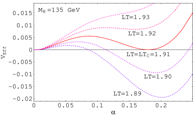
(a)	(b)

Figure 16: (a) Effective potential (for $M_{H}=135\,\textrm{GeV}$) at various temperatures. (b) Detail near the phase transition (localized gauge kinetic terms).

When 5D bulk fermions in very large representations of the gauge group are inserted, so that realistic values of the Higgs mass can be obtained, the first order phase transition becomes weaker and weaker (see figures 9-12). On the other hand, one can get realistic values of the Higgs (and top) mass also by introducing large localized gauge kinetic terms, as discussed in ref. [6]. In this case the strength of the phase transition is considerably increased (see figures 13-16) and could be strong enough to produce a reasonable baryogenesis. A definite result can however be established only by a more careful study of the phase transition, which includes the study of sphalerons and of the possible sources of CP violation in our 5D set-up.

As we have already mentioned, all our results, for any value of $M_{H}<M_{W}$ or $M_{H}\geq M_{W}$, are based on perturbative studies, obtained by computing the one-loop Higgs effective potential. In light of the importance of the correct gauge-fixing procedure, of the higher-loop daisy contributions and of the breakdown of perturbation theory for $M_{H}\gtrsim M_{W}$ in the SM, it is natural to ask if and to what extent one can trust our perturbative one-loop results. To this aim, we show that our 5D one-loop Higgs effective potential is considerably stable under radiative corrections. First of all, we establish that the 5D one-loop Higgs effective potential is gauge independent, by studying a class of background field gauges. This is expected, since the effective action typically fails to be gauge invariant away from its minima, but at tree-level in our model any VEV of the Higgs field is a good minimum, being absent any potential at this order.

We give support to the idea that the phase transition can safely be studied in perturbation theory in Wilson line based models by computing the leading IR divergent daisy contributions to the Wilson line effective potential in a simple 5D model compactified on $S^{1}$. By a comparison between the naïve one-loop thermal mass with the one-loop improved one — obtained by resumming an infinite class of daisy diagrams — we are able to establish that the leading daisy diagrams give a small correction up to temperatures of order $T\sim 1/L$ (see figure 19 (a)) and start to give a relevant contribution only at temperatures of order $T\sim 10/L$ or higher. We take these results as a strong evidence that perturbation theory in 5D models with gauge-Higgs unification is valid also around the critical temperature. The same comparison of one-loop naïve and improved thermal masses is performed in the 4D theory obtained by a trivial dimensional reduction of the 5D model, where only the Kaluza-Klein (KK) zero modes of the fields are retained. This truncation spoils the higher dimensional symmetries responsible for the finiteness of the Wilson line effective potential and indeed, as expected, daisy diagram contributions are larger (see figure 19 (b)).

The paper is organized as follows. In section 2 we show the main features of one-loop effective potentials of Wilson line phases, namely their UV finiteness, gauge independence, high temperature behaviour and establish the generic presence of a first-order phase transition. In section 3 we study the electroweak phase transition in the model of ref. [6], which we briefly review in subsection 3.1. In section 4, the leading higher loop daisy diagrams in an $U(1)$ model coupled with scalars and compactified on $S^{1}$ (and its corresponding model trivially reduced in 4D) are computed. Our conclusions are reported in section 5. Finally, we collect in an appendix all the formulae regarding the contribution to the Wilson line effective potential of bulk fields, with or without possible localized couplings.

2 The Wilson line dynamics at finite temperature

The form of the one-loop effective potential at $T=0$ for Wilson line phases on $S^{1}$ or $S^{1}/{\bf Z}_{2}$ orbifold models is well-known [8, 24]. The non-local nature of Wilson lines imply that their potential is completely UV finite, modulo irrelevant constant vacuum energy terms. This is the most important property of these potentials, which makes the idea of identifying the Higgs field with a Wilson line phase such an interesting proposal to solve the gauge hierarchy problem. We consider below only the effective potential for a single Wilson line phase. Effective potentials for multiple Wilson line phases, however, do not present any problem and are easily obtained by a generalization of that of a single Wilson line phase (see e.g. refs. [8, 25, 26]).

In this class of models, gauge invariance severely constrains the couplings of the gauge field component $A_{5}$ with other fields. In particular, any bulk field couples to $A_{5}$ only through the minimal gauge coupling. In a suitable basis for the fields, each mode $(i)$ couples diagonally with $A_{5}$, giving rise to a simple shift of their KK mass (see e.g. appendix A of ref. [6] for details; all our conventions and notations are as in ref. [6]): $m^{(i)}=(n+q^{(i)}\alpha)/R$, where $n$ is the KK level of the state, $q^{(i)}$ is the charge eigenvalue of the mode $(i)$ and $\alpha$ ($0\leq\alpha\leq 1$) is the VEV of the Wilson line phase. It is related to the zero mode $H$ of $A_{5}$ by the relation $H=2i\alpha/(g_{4}R)$, where $g_{4}$ is the 4D gauge coupling constant, related to the dimensionful 5D gauge coupling constant as follows: $g_{4}=g_{5}/\sqrt{L}$, with $L=2\pi R$.

The effective potential at finite temperature, in the imaginary time formalism, is obtained from that at zero temperature by simply compactifying the Euclidean time direction on a circle of radius $1/(2\pi T)$, where $T$ is the temperature. Fields satisfying Bose/Fermi statistic must be taken to satisfy periodic/anti-periodic boundary conditions along the Euclidean time direction. The bosonic and fermionic contributions to the one-loop Wilson line effective potential at finite temperature are then easily evaluated. For each bosonic and fermionic degree of freedom with charge $q$ and bulk mass term $M$, one has

$$V(T,q\alpha)=\frac{(-)^{2\eta}T}{2}\sum_{k,m=-\infty}^{+\infty}\int\!\frac{d^{3}p}{(2\pi)^{3}}\log\bigg{\{}p^{2}+\bigg{[}2\pi(m+\eta)T\bigg{]}^{2}+M_{k}^{2}(q\alpha)\bigg{\}}\,,$$ (2.1)

where $M_{k}^{2}(q\alpha)=M^{2}+(k+q\alpha)^{2}/R^{2}$ are the masses of the states at KK level $k$, including a possible bulk mass term $M$, $m$ are the Matsubara frequencies and $\eta=0$ or 1/2 for bosons and fermions, respectively. It is important to recall that eq.(2.1) is valid not only for compactifications on $S^{1}$ but also on orbifolds, such as $S^{1}/{\bf Z}_{2}$. In the latter case, the effect of the parity projection in the diagonal basis for the fields amounts simply to reducing the number of physical degrees of freedom with a given charge $q$ with respect to the Wilson line phase. We collect in the appendix several equivalent ways in which one can compute the effective potential (2.1). Notice that eq.(2.1) is valid also for gauge fields $A_{M}$ $(M=0,1,2,3,5)$; in this case one has to take into account a multiplicity factor equal to 3, the number of transverse polarization of a 5D gauge field. Moreover, the gauge contribution is gauge independent. We will discuss in more detail this important aspect in next subsection.

2.1 Gauge independence of the effective potential

The effective potential $V(H_{0})$ in standard spontaneously broken gauge theories, such as the SM, where $H_{0}$ is the VEV of the Higgs field, is generally gauge-dependent [12]. This is easily seen at one-loop level, where the effective potential is obtained by evaluating a trace. In this case one can see, working for instance in an $R_{\xi}$-gauge, that the contributions of the would-be Goldstone bosons, ghosts and longitudinal gauge bosons, outside the minimum for the Higgs field, do not cancel anymore and leave a non-trivial $\xi$-dependent, and thus gauge dependent, term.

In gauge-Higgs unification models, where the Higgs field is identified with the KK zero mode of the gauge field $A_{5}$, such problem does not occur, at least at one-loop level. This is expected since at tree level $A_{5}$ is a modulus, namely any constant value of this field satisfies the equations of motion. In order to show more explicitly the gauge independence of the one-loop effective potential, we define in the following a class of gauge-fixing Lagrangians ${\cal L}_{\xi}$ that are a sort of generalization of the 4D t’Hooft background gauges:

$${\cal L}_{\xi}=-\frac{1}{\xi}{\rm Tr}\,\big{(}\bar{D}_{\mu}A^{\mu}+\xi\bar{D}_{5}A^{5}\big{)}^{2}\,,$$ (2.2)

where $\mu=0,1,2,3$ runs over the 4D directions and $\bar{D}_{M}=\partial_{M}+ig_{5}[\bar{A}_{M},.]$ is the covariant derivative in terms of the classical field configuration $\bar{A}_{M}=\delta_{M5}\alpha/(g_{5}R)\hat{t}$, $\hat{t}$ being the direction in group space where the VEV is aligned. For $\xi=1$, the gauge-fixing term (2.2) reduces to the usual 5D background field gauge commonly used in the literature, to derive the one-loop effective potential of Wilson line phases [8]; for $\xi=0$, we instead get the 4D Landau gauge $\partial_{\mu}A^{\mu}=0$, whereas for $\xi\rightarrow\infty$, eq.(2.2) gives $\bar{D}_{5}A^{5}=0$; the latter condition is precisely the unitary gauge in which all would-be Goldstone bosons associated to the non-linearly realized gauge symmetries are decoupled, as we will see more explicitly in the following. From a 4D point of view, eq.(2.2) is precisely the gauge-fixing term defining an $R_{\xi}$-gauge for the infinite gauge symmetry groups associated to all KK levels of the 5D gauge fields $A_{\mu}(x,y)$. The full 5D Lagrangian for the gauge fields is then

$${\cal L}=-\frac{1}{2}{\rm Tr}\,\big{(}F_{MN}F^{MN}\big{)}+{\cal L}_{\xi}+{\cal L}_{gh}\,,$$ (2.3)

where ${\cal L}_{gh}$ is the ghost Lagrangian associated to the gauge-fixing (2.2):

$${\cal L}_{gh}=-{\rm Tr}\,\big{[}\omega^{*}(\bar{D}_{\mu}D^{\mu}+\xi\bar{D}_{5}D^{5})\omega\big{]}\,.$$ (2.4)

It is not difficult to derive the quadratic Lagrangian, in momentum space, for the gauge, scalar and ghost fields $A_{\mu}$, $A_{5}$ and $\omega$. As discussed before, the only non-trivial task is to derive the linear combination of fields that couples diagonally with $A_{5}$, in which base the effect of the background is simply to shift the KK level of the mode. For definiteness (and because this will be the case we analyze mostly), we consider an $SU(3)$ gauge theory on the orbifold $S^{1}/{\bf Z}_{2}$, where $SU(3)$ is broken by the orbifold parity to $SU(2)_{L}\times U(1)_{Y}$ and thus to $U(1)_{EM}$ by the Wilson line phase $\alpha$. The quadratic Lagrangian of this model reads, in momentum space,

$${\cal L}_{quad.}= \sum_{i=1,2}\sum_{n=-\infty}^{+\infty}\bigg{[}A_{\mu,n}^{(i)^{\dagger}}\Delta_{\mu\nu,n}^{(i)}A_{\nu,n}^{(i)}+A_{5,n}^{(i)^{\dagger}}\Delta_{55,n}^{(i)}A_{5,n}^{(i)}+\omega_{n}^{(i)\dagger}\Delta_{55,n}^{(i)}\omega_{n}^{(i)}\bigg{]}+$$ (2.5)

$$\sum_{i=3,4}\sum_{n=0}^{+\infty}\bigg{[}A_{\mu,n}^{(i)}\Delta_{\mu\nu,n}^{(0)}A_{\nu,n}^{(i)}+A_{5,n}^{(i)}\Delta_{55,n}^{(0)}A_{5,n}^{(i)}+\omega_{n}^{(i)*}\Delta_{55,n}^{(0)}\omega_{n}^{(i)}\bigg{]}\,.$$

In eq.(2.5), the fields $(A_{\mu}^{(1,2)},A_{5}^{(1,2)},\omega^{(1,2)})$ represent the linear combination of fields that couples diagonally to the Higgs field, with charge $q=1,2$. The fields $(A_{\mu}^{(3,4)},A_{5}^{(3,4)},\omega^{(3,4)})$, instead, do not couple to $A_{5}$. The explicit form of these linear combinations of fields, in terms of the usual $SU(3)$ Gell-Mann field decompositions, can be found in Appendix A.3 of ref. [6]. Notice that due to the different ${\bf Z}_{2}$ parities of $A_{\mu}$ and $A_{5}$, we have $A_{5,0}^{(3)}=A_{\mu,0}^{(4)}=\omega_{0}^{(4)}=0$. The inverse propagators are

$$\Delta_{\mu\nu,n}^{(q)}= \eta_{\mu\nu}\bigg{[}p^{2}+\frac{(n+q\alpha)^{2}}{R^{2}}\bigg{]}+\frac{1-\xi}{\xi}p_{\mu}p_{\nu}\,,\ \ \ \ \ \ \ q=0,1,2,$$

$$\Delta_{55,n}^{(q)}= p^{2}+\xi\frac{(n+q\alpha)^{2}}{R^{2}}\,,\hskip 108.12054ptq=0,1,2,$$ (2.6)

where $p^{2}=p_{\mu}p^{\mu}$. It is clear from eq.(2.6) that when $\xi\rightarrow\infty$, all scalar fields $A_{5,n}$ decouple from the theory, with the only exception of $A_{5,0}^{(4)}$, namely the Higgs field. It is now easy to establish the independence on the parameter $\xi$ of the one-loop effective potential. Indeed, for each KK mode level $n$ and charge $q$, the gauge, scalar and ghost contributions give a total factor

$$\frac{\Delta_{55,n}^{(q)}}{\bigg{[}\Delta_{55,n}^{(q)}\,{\rm det}\,\Delta_{\mu\nu,n}^{(q)}\,\bigg{]}^{1/2}}=\sqrt{\xi}\bigg{(}p^{2}+\frac{(n+q\alpha)^{2}}{R^{2}}\bigg{)}^{-\frac{3}{2}}\,,$$ (2.7)

where the determinant in eq.(2.7) is meant to be taken only on the $4\times 4$ polarization matrix of the gauge fields. Aside from the irrelevant $\sqrt{\xi}$ factor, which is reabsorbed in the functional measure, all the non-trivial $\xi$-dependence in eqs.(2.6) cancels out in eq.(2.7), leaving an effective contribution of three scalar degrees of freedom with twist $q$. As stated before, this equals the total contribution of a 5D gauge field $A_{M}$ with the same twist.

The gauge independence of the potential is trivially extended at finite temperature. Indeed, in the imaginary time formalism, eq.(2.7) still holds, the only modification being given by the Matsubara frequency modes, that are all integer-valued for gauge, scalar and ghost fields.

2.2 High temperature behaviour

The one-loop effective potential for Wilson line phases at finite temperature has been computed in ref. [11] (see also ref. [27]), where it has been shown that at temperatures of order $T\sim 1/L$ the symmetry is restored. Its high temperature behaviour is peculiar, as can be seen by studying the bosonic and fermionic contribution to the Higgs thermal mass at $\alpha=0$:

$$M_{H}^{2}(T,\alpha=0)=\bigg{(}\frac{g_{4}R}{2}\bigg{)}^{2}\,\frac{\partial^{2}V}{\partial\alpha^{2}}\bigg{|}_{\alpha=0}\;.$$ (2.8)

For $T\gg 1/L$, the mass (2.8) can easily be extracted from eq.(A.3), using the known asymptotic behaviour of Bessel functions for large values of their argument. For massless bosonic and fermionic bulk fields ($M=0$ in eq.(A.3)) with twist $q$, one finds respectively

$$M_{H}^{2}(T,0)= \frac{g_{4}^{2}}{16\pi^{2}}\left(\frac{2}{3}\pi^{2}q^{2}n_{B}\right)\frac{T}{L}\bigg{\{}1+O\bigg{[}(LT)^{\frac{3}{2}}e^{-2\pi LT}\bigg{]}\bigg{\}}\,,$$ (2.9)

$$M_{H}^{2}(T,0)= -\frac{g_{4}^{2}}{16\pi^{2}}\left(2\sqrt{2}\pi^{2}q^{2}n_{F}\right)\frac{T}{L}(LT)^{\frac{3}{2}}e^{-\pi LT}\bigg{[}1+O\left(\frac{1}{LT}\right)\bigg{]}\,,$$ (2.10)

where $n_{B}$ and $n_{F}$ denote the effective number of bosonic and fermionic degrees of freedom of the field. The exponential terms appearing in eqs.(2.9), (2.10) and the linear temperature dependence of the boson contribution are a characteristic feature of the non-local nature of the Higgs potential. They are different from the typical contributions expected for models in extra dimensions where one gets a thermal mass of order $LT^{3}$ [13], or for the 4D Standard Model, in which the Higgs thermal mass, at high temperatures, goes like $T^{2}$.

The leading high temperature dependence of the one-loop thermal mass can be understood by studying the UV behaviour of the one-loop mass correction at zero temperature. Since this is in general quadratically divergent, power counting implies that its leading finite temperature contribution will be of order $T^{2}$. This counting can also be used in models in extra dimensions. Since at a given $T$, the effective number of KK modes contributing to the thermal ensemble is roughly given by $LT$, one would generally get a leading high temperature contribution to the thermal mass of order $(LT)T^{2}=LT^{3}$, in agreement with ref. [13]. For Wilson line potentials, however, the analysis is different, since they are finite at zero temperature, with a one-loop mass saturated by the compactification scale $1/L^{2}$, times $g_{4}^{2}/(16\pi^{2})$, a 4D loop factor. The non-local nature of the potential is such that all Matsubara mode contributions, but the zero mode one, are exponentially suppressed at high temperatures. The only relevant contribution arises then from bosons, which admit a zero Matsubara mode. Consequently, the thermal mass has a linear dependence on $T$, reproducing the leading term in eq.(2.9). Since the effective number of KK modes contributing in the thermal ensemble is still $LT$, eq.(2.9) can alternatively be understood as the sum of the one-loop, zero temperature, mass corrections of the $(LT)$ KK modes: $(LT)/L^{2}=T/L$. The naïve power counting argument, applied instead to a truncated sum of KK modes, would predict the wrong $LT^{3}$ dependence. In fact, a naïve truncation of the KK sum would spoil the shift symmetry $\alpha\rightarrow\alpha+1$ of the Wilson line phase, resulting also in a fake divergent zero temperature effective potential.

The high T contribution to the Higgs thermal mass of massive bulk fields, with mass $M$, is further exponentially suppressed. In particular, for $M\gg 1/L$, the linear dependence on $T$ appearing in the first term in eq.(2.9) is suppressed by a factor $e^{-ML}$. The same is true for the whole effective potential, as is clear from eq.(A.3). The effective potential is thus exponentially insensitive to UV physics and completely determined by the light 5D degrees of freedom.

Given the high $T$ behaviour of the bosonic and fermionic contributions to the Higgs mass in eqs.(2.9) and (2.10), we can establish on quite general grounds that if a gauge symmetry breaking occurs at $T=0$, namely $M^{2}(T=0,\alpha=0)<0$, it will be restored at a sufficiently high temperature when $M^{2}(T,\alpha=0)\geq 0$. Since Wilson line effective potentials are gauge invariant, $V(-\alpha)=V(\alpha)$, and thus $\alpha=0$ is always an extremum of the potential. Consequently, at sufficiently high $T$, $\alpha=0$ turns to a minimum of the potential, at least locally.

2.3 Properties of the phase transition

An analytical study of the nature of the phase transition occurring in Wilson line based models is not totally straightforward, due to the non-local nature of the order parameter. The essential features of the transition, however, can quantitatively be studied by properly approximating the exact one-loop formulae for the potential appearing in the appendix.

As we will show, the phase transition is typically of first order and is related to the presence of a cubic term in the bosonic contribution of the effective potential. This is very similar to what happens, for instance, in the SM, where a cubic term in the Higgs field appearing in the effective potential at finite temperature is responsible for the generation of a first-order phase transition, for sufficiently low values of the Higgs mass. The cubic term in the Wilson line phase $\alpha$ appears from a high temperature expansion of the bosonic contribution in, say, eq.(A.3). For massless fields with $M=0$, charge $q_{B}$ and for $LT>1$, we can safely drop all Matsubara modes but the zero mode in the sum over $m$ appearing in eq.(A.3). For each degree of freedom, the resulting potential is

$$V_{B}(T,\alpha)\simeq-\frac{T}{\pi^{2}L^{3}}\sum_{\tilde{k}=1}^{\infty}\frac{\cos(2\pi\tilde{k}q_{B}\alpha)}{\tilde{k}^{4}}\,.$$ (2.11)

Interestingly enough, the potential (2.11) admits a very simple polynomial expression in $\alpha$, which can be found by carefully Taylor expanding it in powers of $\alpha$. Since a naïve expansion in $\alpha$ would lead to the appearance of an infinite number of ill-defined sums, a regularization has to be taken to give a meaning to the resulting expression. We will use in the following the $\zeta$-function regularization, according to which $\zeta(-2n)=\sum_{k=1}^{\infty}k^{2n}=0$ for all positive integers $n$. As a consequence, in the expansion of the cosine function in eq.(2.11), all terms but the first three, constant, quadratic and quartic in $\alpha$, vanish. All the odd derivatives in the expansion vanish since $\zeta(-2n+1)$ is finite for $n>0$, but care has to be taken for the third derivative. The latter in fact does not vanish, due to the relation

$$\lim_{x\rightarrow 0^{+}}\sum_{n=1}^{\infty}\frac{\sin(nx)}{n}=\frac{\pi}{2}\,.$$ (2.12)

This is at the origin of the $\alpha^{3}$ term in the expansion of the potential (2.11). It only arises for massless 5D bosonic fields, since for massive fields the sum over $n$ is absolutely convergent, resulting in a trivially vanishing third derivative of the potential.

Putting all terms together and recalling that $\zeta(0)=-1/2$, one gets

$$V_{P}(T,\alpha)=-\frac{\pi^{2}T}{3L^{3}}\bigg{[}\frac{1}{30}-(q_{B}\alpha)^{2}+2(q_{B}\alpha)^{3}-(q_{B}\alpha)^{4}\bigg{]}\,.$$ (2.13)

The expressions (2.11) and (2.13) are identical for $0\leq\alpha\leq 1/q_{B}$. Since $V_{P}(T,q_{B}\alpha=0)=V_{P}(T,q_{B}\alpha=1)$, by periodically extending $V_{P}$ to all values of $\alpha$, one gets a complete identity between the two expressions. Indeed, it is straightforward to check that the Fourier series of the polynomial (2.13) agrees with eq.(2.11). Notice that the $\alpha^{3}$ term is a non-analytic term, since it corresponds to a $(H^{\dagger}H)^{3/2}$ operator, when written in a manifestly gauge-invariant form.

Let us now study how the phase transition schematically occurs in a model with one massless 5D gauge boson and fermion, with charge respectively $q_{B}$ and $q_{F}$ with respect to $\alpha$. We take $q_{F}>q_{B}$, because in this case the analysis is further simplified, as we will see. There is no need to specify, in this simple set-up, which is the underlying theory which gives rise to these fields and to the Wilson line. As a consequence, the analysis is general and it can be applied for any gauge group and compact space ($S^{1}$ or $S^{1}/{\bf Z}_{2}$).

At zero temperature, the effective potential is given by the first row in eq.(A.1) with $M=0$. By summing the fermionic and bosonic contributions, we get

$$V(0,\alpha)=\frac{3}{4\pi^{2}L^{4}}\sum_{\tilde{k}=1}^{\infty}\frac{\big{[}8\cos(2\pi\tilde{k}q_{F}\alpha)-3\cos(2\pi\tilde{k}q_{B}\alpha)\big{]}}{\tilde{k}^{5}}\,.$$ (2.14)

The potential is unstable at $\alpha=0$ and develops a minimum at $\alpha\simeq 1/(2q_{F})$, where the “Higgs mass” is approximately given by

$$M_{H}^{2}\simeq\frac{g_{4}^{2}}{16\pi^{2}}\frac{1}{L^{2}}24q_{F}^{2}\zeta(3)\,,$$ (2.15)

where, as rough approximation, we have neglected the bosonic contribution in eq.(2.15). At finite temperature, as we have already discussed, the fermion contribution is less and less relevant, resulting in a phase transition for $T\sim 1/L$. The transition is more efficiently studied by starting from temperatures slightly above the critical one, when $TL>1$. In this regime, it is a good approximation to use the high temperature expansion for the potential. The bosonic contribution has been already computed and gives rise to the polynomial potential (2.13) multiplied by a multiplicity factor of 3. The fermionic contribution, unfortunately, does not admit a simple finite polynomial expansion which accurately approximates the exact one-loop result, like the bosonic case. As such, a rough approximation will be used to put it in a simple polynomial form. By expanding the modified Bessel functions and retaining only the modes $m=0,-1$ and $\tilde{k}=1$ in eq.(A.3), we roughly get

$$V_{F}(T,\alpha)\simeq\frac{4\sqrt{2}}{L^{4}}(LT)^{5/2}e^{-\pi LT}\cos(2\pi q_{F}\alpha)\,.$$ (2.16)

No $\alpha^{3}$ term arises from the fermion contribution. If we expand the cosine in eq.(2.16) and retain only terms up to $\alpha^{4}$ we see that the effective potential for $LT>1$, resulting by summing $V_{B}$ and $V_{F}$, has the schematic form

$$\frac{L^{4}}{\pi^{2}}V(T,q\alpha)\simeq a(x)\,\alpha^{2}-b(x)\,\alpha^{3}+c(x)\,\alpha^{4}\,,$$ (2.17)

where $x=LT$ and

$$a(x) = q_{B}^{2}x-8q_{F}^{2}\sqrt{2}x^{5/2}e^{-\pi x}\,,$$

$$b(x) = 2xq_{B}^{3}\,,$$ (2.18)

$$c(x) = q_{B}^{4}x+\frac{8}{3}q_{F}^{4}\sqrt{2}\pi^{2}x^{5/2}e^{-\pi x}\,.$$

Eq.(2.17) is valid for $0\leq\alpha\leq 1/(2q_{F})$, which is the relevant range in $\alpha$ for the study of the phase transition. The analysis of the latter for potentials like eq.(2.17) is standard (see e.g. ref. [28]). For $x>>1$, the potential admits only a minimum at $\alpha=0$. As the temperature decreases, an inflection point appears at $T=T_{1}$, below which a non-trivial minimum and maximum appear. The critical temperature $T_{C}$ is defined as the temperature when $V(T_{C},q\alpha_{min}(T_{C}))=0$, namely when the non-trivial minimum is as deep as the minimum at zero. This is given by the largest root of the equation $b^{2}(x_{C})-4a(x_{C})c(x_{C})=0$ which, for $q_{F}>q_{B}$, is nearly equivalent to the vanishing of the term $a(x)$ in eq.(2.17). The critical temperature has only a logarithmic dependence on the charges $q_{B}$ and $q_{F}$ and is of order $1/L$, as mentioned. At $T=T_{C}$, we get

$$\alpha_{min}(x_{C})=\frac{b(x_{C})}{2c(x_{C})}\simeq\frac{6q_{B}}{\pi^{2}q_{F}^{2}}\,.$$ (2.19)

Below the critical temperature $T_{C}$, $\alpha_{min}(T)$ becomes the new global minimum of the potential. The value $|H(T_{C})|/T_{C}=2\alpha_{min}(T_{C})/(g_{4}RT_{C})$ is one of the relevant parameters to study, if one wants to get baryogenesis at the electroweak phase transition (see e.g. ref. [29]). One necessary (but not sufficient) requirement is that $|H(T_{C})|/T_{C}>1$, otherwise sphalerons at $T<T_{C}$ would wash out any previously generated baryon asymmetry [21]. It is also a good parameter to measure the strength of the first-order phase transition. Since the Higgs mass (2.15) is proportional to $q_{F}$, whereas $\alpha_{min}(x_{C})\sim q_{B}/q_{F}^{2}$ and $T_{C}\sim 1/L$, we conclude that

$$\frac{|H(T_{C})|}{T_{C}}\sim\frac{q_{B}}{q_{F}^{2}}\,.$$ (2.20)

The strength of the first-order phase transition is inversely proportional to $q_{F}^{2}$ and hence to the value of the Higgs mass.

In presence of several massless bosonic and fermionic fields, with charges $q_{B,i}$ and $q_{F,i}$, the potential can still be put in the form (2.17), provided that one substitutes in eqs.(2.18) $q_{B}^{k}\rightarrow\sum_{i}n_{B,i}q_{B,i}^{k}$ and $q_{F}^{k}\rightarrow\sum_{i}n_{F,i}q_{F,i}^{k}$, where $n_{B(F),i}$ are the multiplicities of the bosons and fermions with charges $q_{B(F),i}$ ($k=2,3,4$).

For more generic field configurations, such as massive bulk fermions, localized fields or localized gauge kinetic terms, the analytical study of the phase transition is more involved and one has to rely on numerical methods to safely establish its nature. However, since the coefficient $b(x)$ multiplying the $\alpha^{3}$ term in eq.(2.17) will still be non-vanishing (unless the model has no massless bosons coupled to the Wilson line phase), we expect that the phase transition will be of first order. We show in next section that this is what generally happens for the model of ref. [6], by numerically studying the one-loop Higgs potential in a more complicated setting. We will also see that the analytical studies performed in this subsection are still approximately valid.

3 The electroweak phase transition in gauge-Higgs models

In this section, we want to establish the nature of the electroweak phase transition in models with gauge-Higgs unification based on 5D orbifolds. We will consider in particular the model constructed in ref. [6] and study if and how the electroweak phase transition occurs in it and some of its extensions.

3.1 Review of the model

The model of ref. [6] is based on a 5D gauge theory with gauge group $G=SU(3)_{c}\times SU(3)_{w}$ on an $S^{1}/{\bf Z}_{2}$ orbifold. The ${\bf Z}_{2}$ orbifold projection is embedded non-trivially only in the electroweak $SU(3)_{w}$ gauge group, by means of the matrix

$$P=e^{i\pi\lambda_{3}}=\left(\matrix{-1&0&0\cr 0&-1\;\;\,&0\cr 0&0&1\cr}\;\right)\;,$$ (3.1)

where $\lambda_{a}$ are the $SU(3)$ Gell-Mann matrices, normalized as ${\rm Tr}\,\lambda_{a}\lambda_{b}=2\delta_{ab}$. The twist (3.1) breaks the electroweak gauge group in 4D to $SU(2)\times U(1)$. The massless 4D fields are the gauge bosons $A_{\mu}^{a}$ in the adjoint of $SU(2)$ and a charged scalar doublet $H$, the Higgs field, arising from the internal components $A_{5}^{a}$ of the gauge field. A VEV for $A_{5}^{a}$ induces an additional spontaneous symmetry breaking to $U(1)_{EM}$. Following ref. [6], we can take

$$\langle A_{5}^{a}\rangle=\frac{2\alpha}{g_{5}R}\,\delta^{a7}\,,$$ (3.2)

corresponding to a purely imaginary Higgs VEV $\langle H\rangle=2i\alpha/(g_{4}R)$, where $\alpha$ is a Wilson line phase, $0\leq\alpha\leq 1$, and $g_{4}=g_{5}/\sqrt{L}$ is the 4D weak coupling constant.

The exact symmetry $\alpha\rightarrow\alpha+1$ prevents the appearance of any local potential for the Higgs field, at any order in perturbation theory. The only allowed potential terms for the Higgs are non-local in the extra dimension (Wilson lines) and thus free of any divergence [30]. Despite the model is a non-abelian gauge theory in 5D, and thus non-renormalizable, the Higgs potential is insensitive to UV physics and thus calculable. The gauge hierarchy problem is automatically solved in these models.

Introducing matter fields in this set-up is a non-trivial task. One possibility is to introduce massive 5D bulk fermions and massless localized chiral fermions, with a mixing between them, so that the matter fields are identified as the lowest KK mass eigenstates. In this way, a realistic pattern of Yukawa couplings can be obtained [6].

The electroweak phase transition occurs in these models because the radiatively induced one-loop Higgs potential, at zero temperature, is unstable at $\alpha=0$, in presence of matter fields. In the broken phase, the mass of the matter fields is exponentially suppressed in terms of the bulk fermion masses $M_{i}$. Since the contribution to the Higgs potential of massive 5D bulk fermions is also exponentially suppressed in $M_{i}$, effectively the electroweak phase transition is driven by the lightest bulk fermion, the one giving rise, through its mixing with the corresponding localized chiral fermion, to the top quark and top Yukawa coupling. In this sense, the electroweak phase transition is driven by the top quark. We hence focus in the following to the study of the contribution to the Higgs effective potential at finite temperature, given by the gauge fields and by a single bulk fermion, coupled to the boundary fermions which give rise to the top quark. Subsequently, in order to get more realistic values for the Higgs and top mass, as well as for the compactification scale $1/R$, we will consider some extensions of this minimal model, as already suggested in ref. [6].

The bulk 5D fermion that has the correct quantum number to couple with the (conjugate) top quark is the symmetric representation ${\bf 6}$ of $SU(3)_{w}$. More precisely, the matter fermion of this basic construction is as follows. We introduce a couple of bulk fermions $\Psi$ and $\tilde{\Psi}$ with opposite ${\bf Z}_{2}$ parities, in the representation $(\bar{\bf 3},{\bf 6})$ of $SU(3)_{c}\times SU(3)_{w}$. At the orbifold fixed points, we have a left-handed doublet $Q_{L}=(t_{L},b_{L})^{T}$ and a right-handed fermion singlet $t_{R}$ of $SU(2)\times U(1)$. They are located respectively at $y=0$ and $y=L/2$, the two boundaries of the segment $S^{1}/{\bf Z}_{2}$. The parity assignments for the bulk fermions allow for a bulk mass term $M$ mixing $\Psi$ and $\tilde{\Psi}$, as well as boundary couplings $e_{1,2}$ with mass dimension $1/2$ mixing the bulk fermion $\Psi$ to the boundary fermions $Q_{L}$ and $t_{R}$. The matter Lagrangian reads

$$\mathcal{L}_{\rm mat}= \Big{[}\bar{\Psi}\,i\hskip 3.0pt\raisebox{1.0pt}{$/$}D_{5}\,\Psi+\tilde{\bar{\Psi}}\,i\hskip 3.0pt\raisebox{1.0pt}{$/$}D_{5}\,\tilde{\Psi}+\Big{(}\bar{\Psi}M\tilde{\Psi}+\mathrm{h.c.}\Big{)}\Big{]}$$ (3.3)

$$+\,\delta(y)\Big{[}\bar{Q}_{L}\,i\hskip 3.0pt\raisebox{1.0pt}{$/$}D_{4}\,Q_{L}+\Big{(}e_{1}\bar{Q}_{R}^{c}\psi+\mathrm{h.c.}\Big{)}\Big{]}$$

$$+\,\delta(y-\frac{L}{2})\Big{[}\bar{t}_{R}\,i\hskip 3.0pt\raisebox{1.0pt}{$/$}D_{4}\,t_{R}+\Big{(}e_{2}\bar{t}_{L}^{c}\chi+\mathrm{h.c.}\Big{)}\Big{]}\,,$$

where $\psi$ and $\chi$ are the doublet and singlet $SU(2)$ components of the bulk fermion $\Psi$, $\hskip 3.0pt\raisebox{1.0pt}{$/$}D_{4}$ and $\hskip 3.0pt\raisebox{1.0pt}{$/$}D_{5}$ denote the $4D$ and $5D$ covariant derivatives so that $\hskip 3.0pt\raisebox{1.0pt}{$/$}D_{5}=\hskip 3.0pt\raisebox{1.0pt}{$/$}D_{4}+i\gamma_{5}D_{5}$. The exact spectrum of the bulk-boundary fermion system defined by the Lagrangian (3.3) can be determined by solving a complicated trascendental equation. The lighest state is however massless, as long as $\alpha=0$. For $\alpha\neq 0$, the mass $M_{top}$ of the lightest state, that we identify with the top quark, is dynamically generated by non-local Wilson-lines operators, whose coefficients are exponentially suppressed by the bulk mass term $M$. The $W$ mass equals $M_{W}=\alpha/R$, whereas the Higgs mass is radiatively induced and equals

$$M_{H}^{2}(\alpha_{min})=\bigg{(}\frac{g_{4}R}{2}\bigg{)}^{2}\,\frac{\partial^{2}V}{\partial\alpha^{2}}\bigg{|}_{\alpha=\alpha_{min}}\;,$$ (3.4)

with $V(\alpha)$ the zero temperature Higgs effective potential and $\alpha_{min}$ its minimum with the lowest value of $\alpha$. This is typically the global minimum of the potential in the broken phase and is also the first one appearing during the electroweak phase transition. Even when $\alpha_{min}$ is only a local minimum, semiclassical analysis have shown that its tunneling decay rate is negligibly small, leading to a practically stable minimum [25].

Finally, let us comment on the range of validity of this theory as an effective field theory. Using naïve Dimensional Analysis (NDA), we can estimate the UV cut-off scale $\Lambda$ to be given by the scale in which the $5D$ gauge couplings become strong. Using respectively the strong $SU(3)_{c}$ and weak $SU(3)_{w}$ coupling constants, one gets $\Lambda_{c}\sim 10/R$ and $\Lambda_{w}\sim 100/R$ [6].

3.2 Results

We report below our study of the electroweak phase transition in the model of ref. [6] and its generalizations. The results, including all the figures, have been obtained by a numerical computation of the exact one-loop relations reported in the appendix.

3.2.1 Only bulk fields

This is the simplest set-up, in which we consider gauge fields and a couple of bulk fields, with opposite ${\bf Z}_{2}$ parities, in the representation $({\bf 6},\bar{\bf 3})$ of $SU(3)_{w}\times SU(3)_{c}$. No boundary fermions are introduced.

Figure 1: Compactification radius as function of the Higgs mass (only bulk fields).

In this theory, a first order phase transition appears for $\lambda\leq 2.1$, where $\lambda=ML/2$ is the properly rescaled bulk fermion mass, while outside this range no symmetry breaking occurs. The critical temperature of the transition is $T_{C}\sim 1/L$.

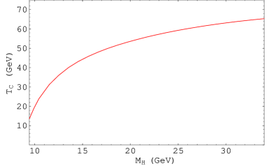
(a)	(b)

Figure 2: (a) Critical temperature and (b) position of the minimum at $T=0$ and at $T=T_{C}$, as function of the Higgs mass (only bulk fields).

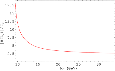
(a)	(b)

Figure 3: (a) Phase transition strength and (b) latent heat as function of the Higgs mass (only bulk fields).

We report in figures 1 and 2 how the compactification radius, the critical temperature and the minimum of the potential (at $T=0$ and at $T=T_{C}$) depend on the Higgs mass, whose value depends on $\lambda$. In figure 3 (a), we plot $|H(T_{C})|/T_{C}$ as function of $M_{H}$. The phase transition is strongly first order, as expected for such low values of $M_{H}$. In figure 3 (b), we plot the latent heat as function of $M_{H}$ (normalized in units of the critical temperature), whose expression is given by

$$\Delta Q=\left.T\frac{\partial}{\partial T}V(T,\alpha_{min})\right|_{T=T_{C}}-\left.T\frac{\partial}{\partial T}V(T,\alpha=0)\right|_{T=T_{C}}\,.$$ (3.5)

For simplicity, we normalize the effective potential so that $V(\alpha=0,T)=0$, in which case the second term in eq.(3.5) vanishes.

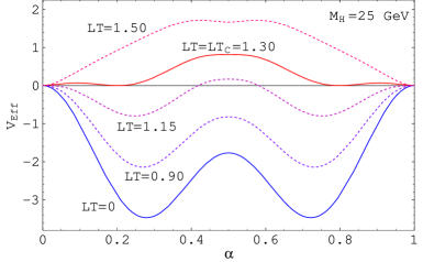
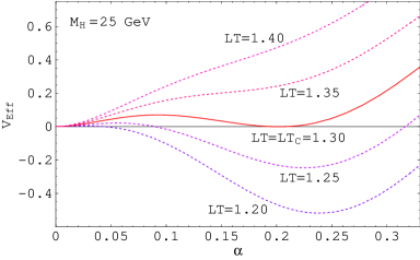
(a)	(b)

Figure 4: (a) Effective potential (for $M_{H}=25\,\textrm{GeV}$) at various temperatures. (b) Detail near the phase transition (only bulk fields).

Finally, in figure 4 we show the shape of the effective potential, for $M_{H}=25\,\textrm{GeV}$, at various temperatures.

For high values of $M_{H}$ (which correspond to low values of the bulk fermion mass $\lambda$), the behaviour of $\alpha_{min}(T_{C})$ and $|H(T_{C})|/T_{C}$ in figures 2 (b) and 3 (a) can be understood by applying the considerations of subsection 2.3. Around the critical temperature the potential (2.17) has only a mild dependence on $\lambda$, at least for $\lambda\lesssim 1.5$, since as first approximation it implies only the shift $\pi LT\rightarrow\sqrt{4\lambda^{2}+(\pi LT)^{2}}$ in eq.(2.16). Hence, although the Higgs mass at $T=0$ is sensibly dependent on $\lambda$, $\alpha_{min}$ and $|H(T_{C})|/T_{C}$, as computed in eqs.(2.19) and (2.20), are essentially independent of $M_{H}$ for low values of $\lambda$ (high values of $M_{H}$).

For larger values of $\lambda$, both $T_{C}$ and $M_{H}$ starts to exponentially depend on $\lambda$, resulting in a linear dependence of $T_{C}$ on $M_{H}$. On the contrary, $\alpha_{min}(T_{C})$ remains still constant. These behaviours are roughly reproduced by the left part of figures 2 (b) and 3 (a).

3.2.2 Inclusion of boundary fermions

We now add the boundary fermions, namely the doublet $Q_{L}$ and the singlet $t_{R}$, as in eq.(3.3). The relevant formulae for the effective potential in presence of boundary fields are found in the appendix, eqs.(A.7). Since the potential does not significantly depend on the bulk-to-boundary coupling $\epsilon_{i}$, the crucial dependence being given by the bulk fermion mass $\lambda$, we have set $\epsilon_{2}=\epsilon_{1}$ and fixed the overall scale by the requirement of having $M_{top}=45\,\mathrm{GeV}$. The effective potential is studied for $0.85\leq\lambda\leq 1.85$. Again, the electroweak phase transition is of first order, with a critical temperature of order $1/L$ (see Figs. 5-8).

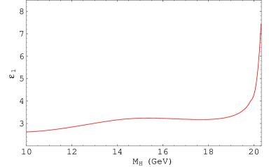
(a)	(b)

Figure 5: (a) Values of the $\epsilon_{1}$ coupling and (b) compactification radius as function of the Higgs mass (inclusion of boundary fermions).

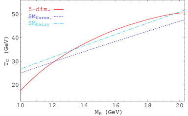
(a)	(b)

Figure 6: (a) Critical temperature and (b) position of the minimum at $T=0$ and at $T=T_{C}$, as function of the Higgs mass (inclusion of boundary fermions).

(a)	(b)

Figure 7: (a) Phase transition strength and (b) latent heat as function of the Higgs mass (inclusion of boundary fermions).

For comparison, in figures 6 (a) and 7, we plotted the critical temperature, $|H(T_{C})|/T_{C}$ and the latent heat as function of the Higgs mass for both the 5D model and the SM, with $M_{top}=45\,\textrm{GeV}$. For the SM case, we plot both the naïve one-loop ($SM_{Unres.}$) and one-loop improved ($SM_{Daisy}$) results, the latter obtained by resumming the leading daisy diagrams [16, 17]. For such low values of the Higgs mass, $10\div 20$ GeV, the SM effective potential is well described by its one-loop approximation.

Even when boundary fermions are inserted, the behaviour of $\alpha_{min}(T_{C})$ and $|H(T_{C})|/T_{C}$ reported in Figures 6 (b) and 7 (a) is very similar to that found in the previous case with only bulk fermions. This is explained by recalling, as already mentioned, that the potential has a small dependence on the bulk-to-boundary couplings $\epsilon_{i}$. All the analytical considerations performed at the end of section 3.2.1 are then approximately valid also in this case.

(a)	(b)

Figure 8: (a) Effective potential (for $M_{H}=18\,\textrm{GeV}$) at various temperatures. (b) Detail near the phase transition (inclusion of boundary fermions).

3.2.3 Theory with high rank bulk fermions

One of the main problems of models based on gauge-Higgs unification is the predicted too low value for the Higgs mass. A possibility to solve this problem is given by the introduction of additional bulk fermions, which do not couple to the localized matter fields, in high rank representations of $SU(3)_{w}$ [6].

(a)	(b)

Figure 9: (a) Value of the $\epsilon_{1}$ coupling and (b) compactification radius, as function of the Higgs mass (high rank bulk fermions).

We consider in the following the electroweak phase transition that one obtains in a 5D model where, in addition to the fields introduced in section 3.2.2, one considers a massive bulk fermion in the completely symmetric rank $8$ representation of $SU(3)_{w}$ and singlet of $SU(3)_{c}$. The mass of this fermion has been fixed to $\lambda_{HR}=2.15$. The bulk-to-boundary couplings $\epsilon_{i}$ have been fixed requiring that $M_{top}=45\,\mathrm{GeV}$, with $\epsilon_{2}=0.5\,\epsilon_{1}$. The effective potential is studied for $1.6\leq\lambda\leq 2.4$. For $\lambda>1.79$ (which corresponds to $M_{H}>125\,\textrm{GeV}$), $\alpha_{min}$ is the global minimum of the potential, which turns to a local minimum for smaller values of $\lambda$. Our results are summarized in figures 9-12.

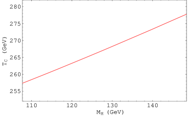
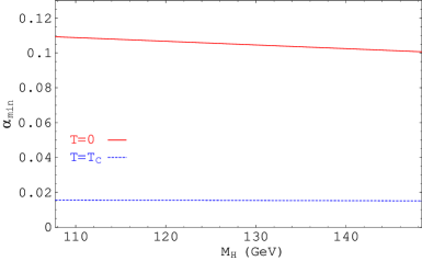
(a)	(b)

Figure 10: (a) Critical temperature and (b) position of the minimum at $T=0$ and at $T=T_{C}$, as function of the Higgs mass (high rank bulk fermions).

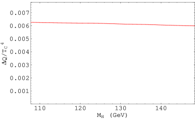
(a)	(b)

Figure 11: (a) Phase transition strength and (b) latent heat as function of the Higgs mass (high rank bulk fermions).

The Higgs mass can now reach realistic values (although the top mass is still too low). As is clear from figure 11 (a), a very weak first order phase transition is found in this model with $T_{C}\sim 1/L$.

This behaviour can be understood by means of our general analysis of section 2.3. The fermionic potential is dominated by the high rank fermion whose mass is fixed. Since $M_{H}$ varies only with $\lambda$, the small dependence on $M_{H}$ in figures 10 (b) and 11 is easily understood. The decreasing of the strength of the phase transition with the rank is clear by noting that

$$\alpha_{min}(T_{C})\sim\frac{\sum_{i}n_{i}q_{i}^{2}}{\sum_{i}n_{i}q_{i}^{4}}\,,$$ (3.6)

where $i$ runs over all the fermion components with charge $q_{i}$ and multiplicity $n_{i}$, arising from the decomposition of the rank $r$ bulk fermion.

Fermions in too high-rank representations can not be considered, since the value of the UV cut-off $\Lambda_{w}$ rapidly decreases as $r$ increases, restricting the range of validity of the effective theory [6]. No comparison with the SM is given, since for such values of the Higgs mass, perturbation theory breaks down close to the critical temperature.

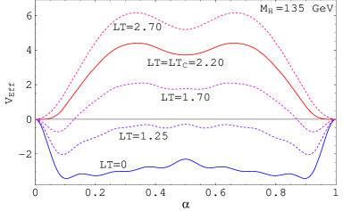
(a)	(b)

Figure 12: (a) Effective potential (for $M_{H}=135\,\textrm{GeV}$) at various temperatures. (b) Detail near the phase transition. The effective potential is multiplied by $10^{4}$ with respect to the (a) diagram (high rank bulk fermions).

3.2.4 Theory with localized gauge kinetic terms

An interesting possibility that is allowed by symmetries in our 5D model is the introduction of localized gauge kinetic terms. These have a significant effect on the phenomenology of models based on gauge-Higgs unification. In particular, they represent another option, in alternative to the introduction of fermions in high rank representations, to get realistic values for the Higgs mass. Interestingly enough, their presence also allow to get acceptable values for the top mass. As a drawback, they break the custodial symmetry, leading to too large deviations for the $\rho$ parameter.

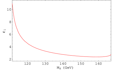
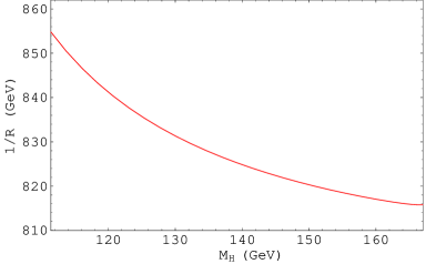
(a)	(b)

Figure 13: (a) Value of the $\epsilon_{1}$ coupling and (b) compactification radius as function of the Higgs mass (localized gauge kinetic terms).

We introduce localized gauge kinetic terms at only one fixed point of $S^{1}/{\bf Z}_{2}$, since this is the most phenomenological convenient option. In the notation of ref. [6], we take $c_{1}\equiv c=6$ and $c_{2}=0$. The gauge contribution to the Higgs effective potential, in presence of localized kinetic terms, is reported in eq.(A.11) of the appendix. The fermions are as in section 3.2.2. The bulk-to-boundary couplings $\epsilon_{i}$ are chosen so that the top quark mass is $110\ \mathrm{GeV}$, with $\epsilon_{2}=\epsilon_{1}$. The effective potential is studied for $0.8\leq\lambda\leq 1.9$. Interestingly enough, despite the high value of the Higgs mass obtained in this case, $110\div 170$ GeV (see figures 13 and 14), the phase transition is still of first order and is also moderately strong, with $|H(T_{C})|/T_{C}\sim 0.7$ (see figure 15 (a)). Since this is of order one, it might be strong enough to avoid that sphalerons in the broken phase wash out the previously generated baryon asymmetry (see footnote 8). The critical temperature in this model is $\sim 2/L$ (see figures 13 (b) and 14 (a)).

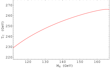
(a)	(b)

Figure 14: (a) Critical temperature and (b) position of the minimum at $T=0$ and at $T=T_{C}$, as function of the Higgs mass (localized gauge kinetic terms).

The behaviour of the phase transition for large values of $c$ is analytically harder to be studied than the previous cases, since the localized gauge field contribution (A.11) plays a crucial role. By expanding the total gauge field contribution, we have been able to establish that the first two terms of the potential in an $\alpha$ expansion, namely the quadratic and cubic term in eq.(2.17), scales like $a(x)\sim 1/c$ and $b(x)\sim c^{-3/2}$. We have not been able to find the asymptotic behaviour for large $c$ of the quartic coupling, which seems to be negative. Neglecting the quartic coupling arising from the bosonic potential, we find that the critical temperature depends only logarithmically on $c$ and $\alpha_{min}(T_{C})\sim 1/\sqrt{c}$. Since $g_{5}\sim g_{4}\sqrt{Lc}$, we get $H(T_{C})/T_{C}\sim 1/c$. Our numerical analysis confirm the decrease of the phase transition strenght with $c$, but numerically we find $|H(T_{C})|/T_{C}\sim 1/c^{1/2\div 1}$, which indicates that the bosonic quartic coupling cannot be totally neglected and result in a slightly stronger first-order phase transition.

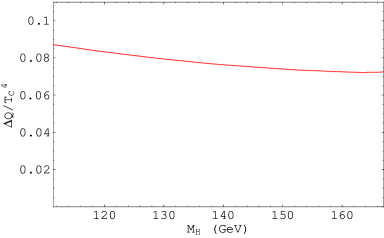
(a)	(b)

Figure 15: (a) Phase transition strength and (b) latent heat as function of the Higgs mass (localized gauge kinetic terms).

4 Estimate of higher-loop corrections

All the analysis performed in this paper about the electroweak phase transition is based on the computation of a one-loop effective potential. Aim of this section is to estimate the leading higher loop contributions and determine the range of validity of our one-loop analysis.

It is known that the most important higher loop contributions to the effective potential in 4D theories generally arise from certain IR divergent diagrams, known as “daisy” or “ring” diagrams [12] (see figure 17).

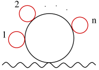
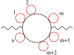
(a)	(b)

Figure 17: Examples of higher loop daisy diagrams contributing to the mass of the Wilson line phase. Solid and wavy lines represent respectively the charged scalar and the Wilson line phase. For simplicity, we have omitted the arrows in the charged scalar propagators.

As shown in ref. [33], the latter are all easily resummed by adding and subtracting to the Lagrangian the one-loop (thermal) mass correction for any field present in the Lagrangian. One then defines a new propagator by adding the thermal mass to the tree level one, and consider the other (opposite) term as a one-loop mass insertion. Such procedure has been performed both at one [16] and two-loop level [17] in the SM. Interestingly enough, the two-loop improved SM effective potential turns out to give results very similar to that computed by numerical results based on lattice simulations even for values of $M_{H}$ close to (but less than) $M_{W}$, in which case perturbation theory is expected to be a bad approximation.

In the following, we will give an estimate of the contribution of daisy diagrams for models where the order parameter is a Wilson line phase, as in theories with gauge-Higgs unification. For simplicity, we focus on a particularly simple model, scalar QED in 5 dimensions, compactified on a circle $S^{1}$ of length $L=2\pi R$. The Lagrangian is

$${\cal L}=(D_{M}\Phi)^{\dagger}D^{M}\Phi-\frac{\lambda_{5}}{4}(\Phi^{\dagger}\Phi)^{2}-\frac{1}{4}F_{MN}F^{MN}\,,$$ (4.1)

where $\Phi$ is a complex scalar field with periodic boundary conditions: $\Phi(2\pi R)=\Phi(0)$. Our aim is to study the effective potential for the Wilson line phase $\alpha=A_{5}g_{5}R$, in the approximation in which the dimensionless 4D gauge coupling $g_{4}\ll\lambda$, with $\lambda=\lambda_{5}/L$. At one-loop order, the effective potential $V(\alpha,T)$ is given by one of the relations reported in the appendix, eqs.(A.3), (A.1) or (A.6), with $d=3$, $M=0$, $\eta=0$ and a factor of 2 taking into account the two scalar degrees of freedom. At higher order, the leading contributions arise from the daisy diagrams drawn in figure 17. Since $g_{4}\ll\lambda$, we can consistently neglect the daisy diagrams involving one-loop mass corrections induced by the gauge field and consider only the one arising from the quartic coupling $\lambda$ (see figure 18).

Let us denote by $I_{n}$ the $(n+1)$-loop daisy diagrams obtained by summing all possible $n$ one-loop mass insertions at zero external 5D momentum and define an effective parameter $\gamma(n)=I_{n}/I_{n-1}$; if there exists some $n$ for which $\gamma(n)\sim 1$ or higher, perturbation theory breaks down and all daisy diagrams must be resummed. It is not difficult to compute $\gamma(n)$ for $n\gg 1$. In this limit, one has to compute only the diagrams (b) in figure 17, since they have a combinatorial factor proportional to $n$, whereas the diagrams (a) have a constant combinatorial factor. Moreover, the $n$ one-loop mass insertions, namely the “small” bubbles in red in figure 17, decouple from the computation and one has only to compute the finite “big” bubble, the one in black in figure 17 (b). We get

$$\gamma(n)\simeq-\left[\frac{LM_{1-loop}(T,\alpha)}{2\pi}\right]^{2}\frac{\sum_{m,k}\bigg{[}(k+\alpha)^{2}+(LT)^{2}m^{2}\bigg{]}^{\frac{-2n-1}{2}}}{\sum_{m,k}\bigg{[}(k+\alpha)^{2}+(LT)^{2}m^{2}\bigg{]}^{\frac{-2n+1}{2}}}\,.$$ (4.2)

In eq.(4.2), $M^{2}_{1-loop}(T,\alpha)$ is the one-loop finite thermal mass correction for the field $\Phi$ which, for $\lambda\gg g$, is given only by the diagram in figure 18 and reads

$$M^{2}_{1-loop}(T,\alpha)=\frac{(LT)T^{2}\lambda}{4\pi^{2}}\sum_{\tilde{k}=1}^{\infty}\sum_{\tilde{m}=-\infty}^{\infty}\frac{\cos(2\pi\alpha\tilde{k})}{\bigg{[}\tilde{m}^{2}+(LT)^{2}\tilde{k}^{2}\bigg{]}^{3/2}}\,.$$ (4.3)

Figure 18: The one-loop mass correction $M^{2}_{1-loop}$ to the charged scalar $\Phi$, induced by the $\lambda(\Phi^{\dagger}\Phi)^{2}$ coupling.

The mass correction (4.3) is defined in a regularization in which only the finite terms arising from the compactification are left, neglecting the UV divergence taken to be equal to that obtained in non-compact 5D space. This is technically achieved by dropping the Poisson resummed $\tilde{k}=0$ term in eq.(4.3). We immediately recognize from eq.(4.2) that for $\alpha\simeq 0$, the leading contribution to $I_{n}$ is given by the KK and Matsubara zero modes $k=m=0$, which give rise to $|\gamma(n)|\sim 1/\alpha^{2}$. The very low values of the Wilson line phase $\alpha$ are the most affected by daisy diagrams, as is obvious by the fact that IR divergences in the diagrams $I_{n}$ appear precisely in the limit $\alpha\rightarrow 0$. A more transparent estimate of the relevance of resumming daisy diagrams can be performed in the two extreme limits when $LT\ll 1$ and $LT\gg 1$. In these two limits, and for sufficiently high $n$, $\gamma(n)\simeq\gamma$ is independent of $n$. For $LT\ll 1$, we can approximate the double sum in eq.(4.2) by taking $k=0$ and substituting the sum over the Matsubara modes with an integral. Viceversa, in eq.(4.3), we can take $\tilde{m}=0$, retain only the sum over the modes $\tilde{k}$ and fix $\alpha=0$. In this way, we get, for $LT\ll 1$,

$$\gamma\simeq-\frac{\lambda\,\zeta(3)}{4\pi^{2}L^{2}}\frac{1}{(\frac{\alpha}{R})^{2}}=-\frac{M^{2}_{1-loop}(0,0)}{M^{2}_{tree}}\,,$$ (4.4)

where $M_{tree}^{2}=(\alpha/R)^{2}$ is the tree-level mass of the lowest KK mode for the field $\Phi$. Daisy diagrams start to be relevant when the thermal mass is of the same order (or higher) than the tree-level one.

For very high temperatures, $LT\gg 1$, the double sums in eq.(4.2) are well approximated by the leading term $k=m=0$, whereas in the mass correction (4.3) we can approximate the sum over $\tilde{m}$ with an integral (setting again $\alpha=0$) and sum over all $\tilde{k}$. One gets, for $LT\gg 1$,

$$\gamma\simeq-\frac{\lambda LT}{48\pi^{2}}\frac{1}{\alpha^{2}}\,.$$ (4.5)

As eq.(4.4), eq.(4.5) can be written as the ratio of the thermal mass at high temperatures over the tree-level mass $M^{2}_{tree}$. In fact, as a rough estimate, obtained by taking $k=m=0$ in the two double sums in eq.(4.2), one sees that at any temperature $\gamma\sim-M^{2}_{1-loop}/M^{2}_{tree}$.

Once established the necessity of considering higher-loop daisy diagrams for sufficiently low values of the Wilson line phase $\alpha$, let us resum all these diagrams by following the procedure outlined in ref. [33]. Since $\gamma<0$, one can expect some cancellation between daisy diagrams of different order, resulting in a decrease of the effect of the daisy resummation procedure. This is indeed what happens, as we will see. As briefly discussed before, along the lines of ref. [33], the resulting one-loop improved effective potential $V_{imp}(T,\alpha)$ is obtained by one of the relations reported in the appendix, eqs.(A.3), (A.1) or (A.6), but by taking $M=M_{1-loop}(T,0)$ instead of $M=0$. From eq.(A.6), for instance, one gets

$$V_{imp}(T,\alpha)=-\frac{4LT^{5}}{(2\pi)^{5/2}}\sum_{\tilde{k}=1}^{\infty}\sum_{\tilde{m}=-\infty}^{\infty}\frac{\cos(2\pi\tilde{k}\alpha)}{\big{[}\tilde{m}^{2}+(LT\tilde{k})^{2}\big{]}^{\frac{5}{2}}}B_{5/2}\bigg{(}\frac{M_{1-loop}(T,0)}{T}\sqrt{\tilde{m}^{2}+(LT\tilde{k})^{2}}\bigg{)}.$$ (4.6)

A good estimate of the higher-order daisy contributions at any temperature is performed by comparing the Wilson line thermal mass obtained from $V_{imp}(T,\alpha)$ with that derived from $V(T,\alpha)$. We denote them respectively $M^{2}_{imp}(T,\alpha)$ and $M^{2}(T,\alpha)$ (not to be confused with $M^{2}_{1-loop}(T,\alpha)$ in eq.(4.3), which is the thermal mass of the field $\Phi$). We plot in figure 19 (a) $M^{2}_{imp}(T,\alpha)$ and $M^{2}(T,\alpha)$ as function of $\alpha$ for $\lambda\sim 1$ and for $LT\sim 1$. As can be seen, the two behaviours are very similar, with deviations which are at most of about 10$\%$ for $\alpha=0$. As expected, the maximal deviation is found for values of $\alpha\simeq 0$. We find that at low temperatures ($LT\sim 1/10$), the maximal deviations (at $\alpha=0$) are of order of a few $\%$, whereas at high temperatures ($LT\sim 10$) they are of order $30\%$. Notice that, although this model does not have a phase transition in the Wilson line parameter, $LT\sim 1$ is in the range of the critical temperature where the phase transition occurs in such kind of models, as we have explicitly seen in sections 2 and 3. From our analysis we thus find that the leading higher-loop daisy diagrams give small corrections to the effective potential. This can be taken as an evidence of the fact that perturbation theory in our 5D models is still valid at $T\sim T_{C}$. On the contrary, for very high temperatures $(LT>>10)$, the one-loop improved potential starts to significantly differ from the naïve one-loop potential. This is particularly evident from the equivalent expression of the potential given in eq.(A.3). At very high temperatures, the naïve one-loop potential is entirely dominated by the Matsubara zero mode $m=0$, proportional to $T$, whereas the one-loop improved potential, due to the non-vanishing argument in the function $B_{2}$ appearing in eq.(A.3), is exponentially suppressed in $LM\simeq\sqrt{LT}$. The discrepancy that one finds between the two potentials starts however to be very large for temperatures which are well above the cut-off scale $\Lambda$. As discussed in footnote 6, it is meaningless to consider such range of temperatures in an effective field theory approach.

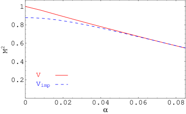
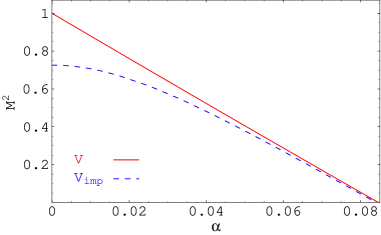
(a)	(b)

Figure 19: (a) Thermal masses in 5D, from the one-loop naïve potential (red solid line) and the one-loop improved one (blue dashed line). (b) Thermal masses in the reduced 4D model, from the one-loop naïve potential (red solid line) and the one-loop improved one (blue dashed line). In both cases the normalization is such that $M^{2}(\alpha=0,T)=1$.

It is useful to compare the contribution of daisy diagrams for the 5D $U(1)$ model above with that of the 4D model arising by trivial dimensional reduction, where all the massive KK modes are neglected. By denoting with $a$ and $\phi$ the properly normalized zero mode components of $A_{5}$ and $\Phi$, one gets the following 4D Lagrangian:

$${\cal L}=(D_{\mu}\phi)^{\dagger}D^{\mu}\phi+\frac{1}{2}(\partial_{\mu}a)(\partial^{\mu}a)-g^{2}\,a^{2}\,\phi^{\dagger}\phi-\frac{\lambda}{4}(\phi^{\dagger}\phi)^{2}-\frac{1}{4}F_{\mu\nu}F^{\mu\nu}\,.$$ (4.7)

The trivial dimensional reduction spoils the 5D Wilson line nature of $\alpha$, breaking the shift symmetry $\alpha\rightarrow\alpha+1$. Let us study the effective potential $V(\alpha)$ for the VEV of the field $a$ ($\langle a\rangle=\alpha/(gR)$). The contribution of $\Phi$ to $V(\alpha)$ is the standard one for a massive scalar field at finite temperature [12]. One has, neglecting terms independent of $\alpha$,

$$V(T,\alpha)=V(0,\alpha)+\frac{T^{4}}{\pi^{2}}\int_{0}^{\infty}\!dx\,x^{2}\log\bigg{[}1-e^{-\sqrt{x^{2}+(\alpha/RT)^{2}}}\bigg{]}\,.$$ (4.8)

In eq.(4.8), $V(0,\alpha)$ is the zero temperature effective potential, which is UV divergent. In the $\overline{{\rm MS}}$ regularizatrion scheme, it reads

$$V(0,\alpha)=\frac{\alpha^{4}\pi^{2}}{2L^{4}}\bigg{[}\log\left(\frac{\alpha^{2}}{R^{2}\mu^{2}}\right)-\frac{3}{2}\bigg{]}\,,$$ (4.9)

where $\mu$ is the renormalization scale.

The one-loop improved potential is obtained by substituting in eq.(4.8) the tree-level mass with the one-loop improved one, computed in the 4D reduced model. For $g\ll\lambda$, this simply amounts to shifting $(\alpha/R)^{2}\rightarrow(\alpha/R)^{2}+\lambda T^{2}/12$. We plot the thermal masses obtained by the one-loop naïve and improved potentials in figure 19 (b) for $LT\sim 1$, $\lambda\sim 1$ and setting $\mu=1/R$, which is the scale above which our effective theory breaks down. The comparison between figures 19 (a) and (b) clearly indicates that the 5D model is less sensitive to higher-loop effects than the 4D reduced theory, although both models are not much sensitive to the daisy resummation procedure for $\alpha\gtrsim 0.05$.

Let us now comment on the daisy diagram contributions to the Higgs effective potential in 5D gauge-Higgs unification models where no fundamental scalars are present. Fermion loops do not give rise to IR divergencies since the Matsubara modes are half integers and there is always an effective non-vanishing thermal mass. Moreover, chiral symmetry implies that fermion mass corrections are always proportional to their tree-level mass and thus they vanish in the IR limit of vanishing mass. There is then no need of resumming daisy diagrams for fermions. Gauge invariance forbids the appearance of any thermal mass correction to the transverse polarization of gauge bosons which are also unaffected by the daisy resummation procedure. The Higgs field itself, $H$, does not have tree-level self-interactions and hence does not give any higher-loop contribution to its potential in the daisy approximation. Finally, we are left with the longitudinal components $A_{0}$ of the gauge fields, that acquire a non-vanishing thermal mass correction (Debye mass); the corresponding contributions to the Higgs potential have to be daisy-resummed. We expect that the latter will be of the same order of magnitude as the one we have estimated in our simple 5D model defined by the Lagrangian (4.1).

As it happens in the SM, we might expect that the resummation of daisy diagrams in our 5D model leads to a change in the cubic term of the approximate Wilson line potential (2.17). However, since transverse gauge bosons are not unaffected by daisy diagrams, this shift would only lead to a slight change of the potential, which will still predict a first-order phase transition.

As final remark, note that the absence of a tree-level potential in Wilson line based models permits to evade Weinberg’s rough argument for the necessity of the breakdown of perturbation theory around the phase transition [34]: since the tree-level potential appearing in generic quantum field theories is temperature independent, perturbative corrections (which are instead temperature-dependent) cannot give rise to a drastic change in the potential (as needed for a phase transition), unless perturbation theory breaks down.

5 Conclusions

We have studied various aspects of the dynamics of Wilson line phases at finite temperature. From a more theoretical viewpoint, we have first of all shown that the one-loop effective potential is gauge invariant, contrary to ordinary effective potentials in non-abelian gauge theories in 4D, including the SM. We have also pointed out that the non-local nature of the Wilson line potential, which already ensures its finiteness at zero temperature at all orders in perturbation theory, is responsible for its mild dependence on quantum corrections at finite temperature. We have established this result by computing the one-loop improved thermal mass — obtained by resumming certain IR divergent higher loop diagrams — with the naïve one in a given 5D model, and showing that the improvement obtained by the resummation is small. This gives strong evidence that in models in which the order parameter is given by a Wilson line phase (models of gauge-Higgs unification), perturbation theory generally holds at least up to the critical temperature $T_{C}\sim 1/L$. Of course, it would be interesting and reassuring to establish this result by performing a systematic study of higher loop corrections for these 5D models.

At a more phenomenological level, we have studied how the phase transition occurs in Wilson line based models, showing that this is typically of first-order. We have then focused our attention to a particular model [6], in which the Wilson line phase transition is identified with the electroweak phase transition. In this model, unless some generalizations are considered, the Higgs mass is always predicted to be too low: $M_{H}<M_{W}/2$. In this range, the transition is strongly of first order, similarly to what happens for the SM in the same regime of parameters.

Introducing bulk fermions in large representations of the $SU(3)_{w}$ gauge group allow for reasonable Higgs masses. In this case, the first order phase transition is very weak and most likely unable to give a successful electroweak baryogenesis. Another possible option to increase the Higgs mass is obtained by introducing large localized gauge kinetic terms. Interestingly enough, the first order phase transition is now considerably stronger than in the previous case and it might even be sufficiently strong for electroweak baryogenesis.

We tacitly assumed in our paper that the dynamics of Wilson line phases at finite temperature is decoupled from that of space-time itself, namely that the mechanism stabilizing the internal direction does not alter our analysis or takes place at temperatures higher than the critical temperature $T_{C}$. Since the compactification scale is of the same order of $T_{C}$, it would be interesting to see in some concrete model of radius stabilization if this assumption can actually be verified.

Appendix A Explicit form of the potential

A.1 Bulk fields contribution

There are various ways of computing eq.(2.1) for bulk fields. For generality, we will report in the following the result that one obtains in $d$ non-compact dimensions. A possible computation is to disentangle the $T=0$ and $T\neq 0$ terms in eq.(2.1) and compute the $T$-dependent term as usually done in 4D for each KK state. In this case, one simply gets (see i.e. [12, 17])

$$V(T,q\alpha)=V(T=0,q\alpha)+(-)^{2\eta}\,T\sum_{k=-\infty}^{+\infty}\int\!\frac{d^{d}p}{(2\pi)^{d}}\log\bigg{[}1-(-)^{2\eta}e^{-\frac{\sqrt{p^{2}+M_{k}^{2}}}{T}}\bigg{]}\,,$$ (A.1)

where $p^{2}$ denotes the $d$ dimensional non-compact momentum square.

Other useful and more explicit forms of the potential are obtained by using the relation ${\rm tr}\,\log A=-\int_{0}^{\infty}dt/t\,{\rm tr}\,e^{-tA}$ in eq.(2.1), valid up to irrelevant constants. Subsequently, one can use the Poisson resummation formula

$$\sum_{n=-\infty}^{+\infty}e^{-\pi t(n+a)^{2}}=\frac{1}{\sqrt{t}}\sum_{\tilde{n}=-\infty}^{+\infty}e^{-\frac{\pi\tilde{n}^{2}}{t}}e^{2i\pi\tilde{n}a}\,.$$ (A.2)

The above formula can be applied in eq.(2.1) to the KK modes $k$, to the Matsubara ones $m$, or to both, resulting in different but equivalent ways of computing the effective potential. In the three cases, one gets, respectively:

$$V(T,q\alpha)=\frac{2T(-)^{2\eta-1}}{(2\pi)^{\frac{d+1}{2}}L^{d}}\sum_{\tilde{k}=1}^{\infty}\sum_{m=-\infty}^{\infty}\frac{\cos(2\pi\tilde{k}q\alpha)}{\tilde{k}^{d+1}}B_{\frac{d+1}{2}}\bigg{[}L\tilde{k}\sqrt{M^{2}+[2\pi(m+\eta)T]^{2}}\bigg{]}\,,\\$$ (A.3)

where

$$B_{\frac{d+1}{2}}(x)\equiv x^{\frac{d+1}{2}}K_{\frac{d+1}{2}}(x)$$ (A.4)

and $K_{n}$ are the modified Bessel functions. By Poisson resumming over $m$, we get

$$V(T,q\alpha) = (-)^{2\eta-1}\frac{L}{\pi(2\pi)^{\frac{d}{2}}}\sum_{\tilde{k}=1}^{\infty}\frac{\cos(2\pi\tilde{k}q\alpha)}{(L\tilde{k})^{d+2}}B_{\frac{d+2}{2}}(LM\tilde{k})+$$

$$2(-)^{2\eta-1}\sum_{k=-\infty}^{\infty}\sum_{\tilde{m}=1}^{\infty}(-)^{2\tilde{m}\eta}\left(\frac{T}{\tilde{m}\sqrt{2\pi}}\right)^{d+1}\!\!B_{\frac{d+1}{2}}\bigg{(}\frac{M_{k}\tilde{m}}{T}\bigg{)}\,,$$

where a Poisson resummation over $k$ has been performed in the first term ($\tilde{m}=0$). Finally, by Poisson resumming in both indices, one finds

$$V(T,q\alpha) = (-)^{2\eta-1}\frac{LT^{d+2}}{\pi(2\pi)^{\frac{d}{2}}}\sum_{\tilde{k}=1}^{\infty}\sum_{\tilde{m}=-\infty}^{\infty}(-)^{2\eta\tilde{m}}\bigg{[}\tilde{m}^{2}+(LT\tilde{k})^{2}\bigg{]}^{-\frac{d+2}{2}}$$ (A.6)

$$B_{\frac{d+2}{2}}\bigg{[}\frac{M}{T}\sqrt{\tilde{m}^{2}+(LT\tilde{k})^{2}}\bigg{]}\cos(2\pi\tilde{k}q\alpha)\,.$$

In eqs.(A.3),(A.1) and (A.6) an irrelevant $\alpha$-independent term has always been omitted. All these relations also hold for vanishing bulk mass term, $M=0$, by noticing that $\lim_{x\rightarrow 0}B_{\alpha}(x)=2^{\alpha-1}\Gamma(\alpha)$, where $\alpha$ is any positive integer or half-integer number.

A.2 Boundary-bulk fields contribution

The contribution to the Higgs effective potential of bulk and boundary fields mixed as in eq.(3.3) is substantially more involved than that of purely bulk fields. One has essentially to compute $V(T,q\alpha)$ directly from eq.(2.1), where $M_{k}^{2}$ are the mass eigenvalues of the bulk-boundary system. It turns out that the full contribution can be written as a sum of a purely bulk contribution and a remaining boundary term. For the matter Lagrangian (3.3), the bulk contribution is that given by the bulk fermions $\Psi$ and $\tilde{\Psi}$ with $e_{1}=e_{2}=0$, whereas the boundary contribution is a simple generalization of the one found in ref. [6] at $T=0$:

$$V_{u}(T,\alpha) = -\frac{8T}{\pi^{2}L^{3}}\sum_{m=-\infty}^{+\infty}\int_{0}^{\infty}dx\,x^{2}\ln\Bigg{[}\prod_{i=1}^{2}\mathrm{Re}\bigg{[}1+\delta_{i2}\frac{{\epsilon_{2}}^{2}}{2\widetilde{x}_{\lambda}}f_{0}(\widetilde{x}_{\lambda},0)$$

$$+\frac{{\epsilon_{i}}^{2}}{2^{\delta_{i2}}\widetilde{x}_{\lambda}}f_{0}(\widetilde{x}_{\lambda},2\alpha)\bigg{]}+\prod_{i=1}^{2}\mathrm{Im}\bigg{[}\frac{{\epsilon_{i}}^{2}}{2^{\delta_{i2}}\widetilde{x}}f_{1}(\widetilde{x}_{\lambda},2\alpha)\bigg{]}\Bigg{]},$$

$$V_{d}(T,\alpha) = -\frac{8T}{\pi^{2}L^{3}}\sum_{m=-\infty}^{+\infty}\int_{0}^{\infty}dx\,x^{2}\ln\Bigg{[}\prod_{i=1}^{2}\mathrm{Re}\bigg{[}1+\delta_{i1}\frac{{\epsilon_{1}}^{2}}{2\widetilde{x}_{\lambda}}f_{0}(\widetilde{x}_{\lambda},\alpha)\bigg{]}\Bigg{]}\,.$$ (A.7)

In eq.(A.7), $\lambda=ML/2$ and $\epsilon_{1,2}=\sqrt{L}e_{i}/2$ are dimensionless parameters defined from the bulk mass $M$ and mixing terms $e_{i}$ appearing in eq.(3.3),

$$\widetilde{x}^{2}\equiv x_{0}^{2}+x^{2}\quad\textrm{and}\quad\widetilde{x}_{\lambda}^{2}\equiv(x_{0}^{2}+x^{2}+\lambda^{2}),$$ (A.8)

and $x_{0}=(m+1/2)\pi LT$ is the properly rescaled Matsubara frequence for a fermion. The functions $f_{0,1}$ are defined as in ref. [6]:

$$f_{0}(\widetilde{x}_{\lambda},\alpha) = \sum_{n=-\infty}^{\infty}\frac{1}{\widetilde{x}_{\lambda}+i\pi(n+\alpha)}=\coth(\widetilde{x}_{\lambda}+i\pi\alpha)\;,$$ (A.9)

$$f_{1}(\widetilde{x}_{\lambda},\alpha) = \sum_{n=-\infty}^{\infty}\frac{(-1)^{n}}{\widetilde{x}_{\lambda}+i\pi(n+\alpha)}=\sinh^{-1}(\widetilde{x}_{\lambda}+i\pi\alpha)\;.$$ (A.10)

In presence of localized gauge kinetic terms, the gauge field contribution is given by the sum of the purely bulk term and an additional boundary term. The latter, for a field which couples diagonally with the Higgs field with charge $q$, can be written as

$$V_{g}^{c_{i}}(T,q\alpha)=\frac{6T}{\pi^{2}L^{3}}\sum_{m=-\infty}^{+\infty}\int_{0}^{\infty}\!\!dx\,x^{2}\ln\left[\prod_{i=1}^{2}\mathrm{Re}\left[1+c_{i}\widetilde{x}f_{0}(\widetilde{x},q\alpha)\right]-\prod_{i=1}^{2}\mathrm{Re}\left[c_{i}\widetilde{x}f_{1}(\widetilde{x},q\alpha)\right]\right],$$ (A.11)

with $\widetilde{x}$ defined as in eq.(A.8), but with $x_{0}=m\pi LT$.

References

- [1]
-
[2]
I. Antoniadis,
Phys. Lett. B 246 (1990) 377;
I. Antoniadis, C. Munoz, M. Quiros, Nucl. Phys. B 397 (1993) 515 [hep-ph/9211309];
I. Antoniadis, S. Dimopoulos, A. Pomarol, M. Quiros, Nucl. Phys. B 544 (1999) 503;
A. Delgado, A. Pomarol, M. Quiros, Phys. Rev. D 60 (1999) 095008 [hep-ph/9812489]. -
[3]
N. S. Manton,
Nucl. Phys. B 158 (1979) 141;
D. B. Fairlie, Phys. Lett. B 82 (1979) 97; J. Phys. G 5 (1979) L55;
P. Forgacs, N. S. Manton, Commun. Math. Phys. 72 (1980) 15;
S. Randjbar-Daemi, A. Salam, J. Strathdee, Nucl. Phys. B 214 (1983) 491;
N. V. Krasnikov, Phys. Lett. B 273 (1991) 246;
H. Hatanaka, T. Inami, C. Lim, Mod. Phys. Lett. A 13 (1998) 2601 [hep-th/9805067]. -
[4]
L. J. Hall, Y. Nomura, D. R. Smith,
Nucl. Phys. B 639 (2002) 307
[hep-ph/0107331];
G. Burdman, Y. Nomura, Nucl. Phys. B 656 (2003) 3 [hep-ph/0210257];
N. Haba, Y. Shimizu, Phys. Rev. D 67 (2003) 095001 [hep-ph/0212166];
K. w. Choi et al., JHEP 0402 (2004) 037 [arXiv:hep-ph/0312178];
I. Gogoladze, Y. Mimura, S. Nandi, Phys. Lett. B 560 (2003) 204 [hep-ph/0301014];
ibid. 562 (2003) 307 [hep-ph/0302176]; Phys. Rev. D 69 (2004) 075006. -
[5]
G. R. Dvali, S. Randjbar-Daemi, R. Tabbash,
Phys. Rev. D 65 (2002) 064021
[hep-ph/0102307];
I. Antoniadis, K. Benakli, M. Quiros, New J. Phys. 3 (2001) 20 [hep-th/0108005];
C. Csaki, C. Grojean, H. Murayama, Phys. Rev. D 67 (2003) 085012 [hep-ph/0210133];
C. A. Scrucca, M. Serone, L. Silvestrini and A. Wulzer, JHEP 0402 (2004) 049. - [6] C. A. Scrucca, M. Serone, L. Silvestrini, Nucl. Phys. B 669 (2003) 128 [hep-ph/0304220].
- [7] J. Scherk and J. H. Schwarz, Phys. Lett. B 82 (1979) 60.
- [8] Y. Hosotani, Phys. Lett. B 126 (1983) 309; ibid. 129 (1983) 193; Ann. Phys. 190 (1989) 233.
-
[9]
E. Witten,
Nucl. Phys. B 258 (1985) 75;
L. E. Ibáñez, H. P. Nilles, F. Quevedo, Phys. Lett. B 187 (1987) 25. - [10] K. Agashe, R. Contino and A. Pomarol, “The minimal composite Higgs model,” arXiv:hep-ph/0412089.
- [11] C. L. Ho and Y. Hosotani, Nucl. Phys. B 345 (1990) 445.
- [12] L. Dolan and R. Jackiw, Phys. Rev. D 9 (1974) 3320.
- [13] K. R. Dienes, E. Dudas, T. Gherghetta and A. Riotto, Nucl. Phys. B 543 (1999) 387.
- [14] J. R. Espinosa, M. Losada and A. Riotto, “Symmetry nonrestoration at high temperature in little Higgs models,” arXiv:hep-ph/0409070.
- [15] D. A. Kirzhnits, JETP Lett. 15 (1972) 529 [Pisma Zh. Eksp. Teor. Fiz. 15 (1972) 745]; D. A. Kirzhnits and A. D. Linde, Phys. Lett. B 42 (1972) 471.
- [16] M. E. Carrington, Phys. Rev. D 45 (1992) 2933.
- [17] P. Arnold and O. Espinosa, Phys. Rev. D 47 (1993) 3546 [Erratum-ibid. D 50 (1994) 6662] [arXiv:hep-ph/9212235].
- [18] M. Laine, Phys. Lett. B 335 (1994) 173 [arXiv:hep-ph/9406268].
- [19] W. Buchmuller, Z. Fodor and A. Hebecker, Phys. Lett. B 331 (1994) 131 [arXiv:hep-ph/9403391]; Nucl. Phys. B 447 (1995) 317 [arXiv:hep-ph/9502321]; A. Hebecker, “The Electroweak phase transition,” arXiv:hep-ph/9506418.
- [20] K. Kajantie, M. Laine, K. Rummukainen and M. E. Shaposhnikov, Phys. Rev. Lett. 77 (1996) 2887 [arXiv:hep-ph/9605288].
-
[21]
V. A. Kuzmin, V. A. Rubakov and M. E. Shaposhnikov,
Phys. Lett. B 155 (1985) 36;
A. G. Cohen, D. B. Kaplan and A. E. Nelson, Ann. Rev. Nucl. Part. Sci. 43 (1993) 27 [arXiv:hep-ph/9302210]. -
[22]
C. Grojean, G. Servant and J. D. Wells,
“First-order electroweak phase transition in the standard model with a low
cutoff,”
arXiv:hep-ph/0407019;
S. W. Ham and S. K. Oh, Phys. Rev. D 70 (2004) 093007 [arXiv:hep-ph/0408324];
D. Bodeker, L. Fromme, S. J. Huber and M. Seniuch, “The baryon asymmetry in the standard model with a low cut-off,” arXiv:hep-ph/0412366. - [23] M. Carena, A. Megevand, M. Quiros and C. E. M. Wagner, “Electroweak baryogenesis and new TeV fermions,” arXiv:hep-ph/0410352.
- [24] M. Kubo, C. S. Lim and H. Yamashita, Mod. Phys. Lett. A 17, 2249 (2002).
- [25] N. Haba, M. Harada, Y. Hosotani and Y. Kawamura, Nucl. Phys. B 657 (2003) 169 [Erratum-ibid. B 669 (2003) 381] [arXiv:hep-ph/0212035].
- [26] N. Haba and T. Yamashita, JHEP 0402 (2004) 059 [arXiv:hep-ph/0401185].
- [27] K. Shiraishi, Z. Phys. C 35 (1987) 37.
- [28] G. W. Anderson and L. J. Hall, Phys. Rev. D 45 (1992) 2685.
- [29] M. Quiros, “Finite temperature field theory and phase transitions,” arXiv:hep-ph/9901312.
-
[30]
N. Arkani-Hamed et al.,
Nucl. Phys. B605 (2001) 81
[hep-ph/0102090];
A. Masiero, C. A. Scrucca, M. Serone, L. Silvestrini, Phys. Rev. Lett. 87 (2001) 251601 [hep-ph/0107201]. - [31] M. Serone and A. Wulzer, “Orbifold resolutions and fermion localization,” arXiv:hep-th/0409229.
-
[32]
K. Kajantie, M. Laine, K. Rummukainen and M. E. Shaposhnikov,
Nucl. Phys. B 466 (1996) 189 [arXiv:hep-lat/9510020];
F. Csikor et al., Nucl. Phys. B 474 (1996) 421. - [33] R. R. Parwani, Phys. Rev. D 45 (1992) 4695 [Erratum-ibid. D 48 (1993) 5965].
- [34] S. Weinberg, Phys. Rev. D 9 (1974) 3357.