Simulated annealing for generalized Skyrme models

Abstract

We use a simulated annealing algorithm to find the static field configuration with the lowest energy in a given sector of topological charge for generalized $SU(2)$ Skyrme models. These numerical results suggest that the following conjecture may hold: the symmetries of the soliton solutions of extended Skyrme models are the same as for the Skyrme model. Indeed, this is verified for two effective Lagrangians with terms of order six and order eight in derivatives of the pion fields respectively for topological charges $B=1$ up to $B=4$. We also evaluate the energy of these multi-skyrmions using the rational maps ansatz. A comparison with the exact numerical results shows that the reliability of this approximation for extended Skyrme models is almost as good as for the pure Skyrme model. Some details regarding the implementation of the simulated annealing algorithm in one and three spatial dimensions are provided.

I Introduction

The Skyrme model Skyrme1961 was originally formulated to provide a description of baryons as topological solitons of finite energy emerging in the framework of a nonlinear theory of weakly coupled pions fields. Nowadays, this idea is partly supported by the $1/N_{c}$ analysis 'tHooft1974 ; Witten1979 , according to which the low-energy limit of QCD could be represented by an effective theory of infinitely many mesons fields whose derivatives appear to all-orders. Since little is known about the exact form of such a Lagrangian, significant efforts have been made to formulate in a simple way Skyrme-like effective Lagrangians Jackson1985 ; Marleau1990 . It was then possible to improve the phenomenological predictions for the spherically symmetric skyrmion with unit topological charge $(B=1)$ DubeMarleau1990 ; Jackson1991 with higher order Lagrangians, whereas only a relative accord with experimental data was achieved with the original Skyrme model Adkins1983 .

On the other hand, analysis based on axially symmetric ansatz Kopeliovich1987 ; Bratten1988 and full numerical studies Bratten1990 ; Battye19971 ; Battye19972 have shown that the angular distribution of static Skyrme fields is not accurately reproduced by the spherically symmetric hedgehog ansatz in the general context of topological charges $B>1$. For the case of models containing higher order terms, not much is known for these $B>1$ and the angular configuration of skyrmions needs to be investigated in greater details. A few steps towards this has been made in Kopeliovich1987 and more recently in Floratos2001 for a Skyrme model extended to order six in derivatives of the pion fields assuming an axially symmetric solution.

In this work, we use a simulated annealing algorithm to minimize the static energy functional of order six and order eight extended Skyrme models for baryonic numbers $B=1$ to $B=4$, following the approach in Hale2000 where this numerical method was used to solve the Skyrme model. No specific ansatz is used to get the minimum energy solutions. The essence of simulated annealing (SA) relies on the analogy that can be made with a solid which is slowly cooled down, stating that if thermal equilibrium is achieved at each temperature during the cooling process, the solid will eventually reach its ground state. The first application of this idea to optimization problems like the minimization of energy functionals has been demonstrated in Kirkpatrick1983 . We use a similar strategy where SA describes the cooling process of our system and a Metropolis algorithm Metropolis1953 brings it into thermal equilibrium. The main advantage of this method over other techniques is that it only involves the energy density and there is no need to write or solve directly a set of differential equations that become more complex as the order of the Lagrangian increases.

The exact soliton solutions that we obtain with the SA algorithm also constitute a valuable comparison tool to study the rational maps approximation for Skyrme fields in the case of generalized models. This approximation works quite well for the Skyrme model Houghton1998 ; Battye2002 , and one might conjecture that a rational map based ansatz would accurately depict the solutions of extended Skyrme models in general. Interestingly, it has been demonstrated that adding a sixth order term in derivatives of the pion fields to the Skyrme Lagrangian does not compromise the reliability of the rational maps ansatz Floratos2001 . Conversely, when a pion mass term is introduced, the symmetries of the skyrmions differ from those of the original Skyrme model for higher topological sectors Battye2004 , making the use of rational maps inappropriate. Thus, it is pertinent to test further this ansatz for other extensions of the Skyrme model.

In the next section, we give a brief account on the structure of the Skyrme model and some of its extensions. Then, in section III, we review the rational maps ansatz and use it to write a static energy functional for generalized Skyrme models. As an aside, we introduce a new positivity constraint on the models proposed in DubeMarleau1990 ; Jackson1991 in section IV. Comparison with rational maps ansatz requires a finite order Lagrangian, which motivates our choice to restrict our analysis to order-six and order-eight models. Section V provides a rather detailed description of the SA algorithm we use in three spatial dimensions, leading to exact soliton solutions, and the one we use in one spatial dimension to minimize the radial energy functional of the skyrmion, where the angular dependence has already been integrated out as a result of the use of rational maps. Finally, we discuss the validity and the limits of our SA results in section VI, where we also draw conclusions concerning the symmetries of the skyrmions we obtain and the reliability of the rational maps ansatz.

II Generalized Skyrme models

The $SU(2)$ Skyrme model Lagrangian density for zero pion mass takes the form

$$\mathcal{L}_{S}=-\frac{F_{\pi}^{2}}{16}~{}\mathrm{Tr}L_{\mu}L^{\mu}+\frac{1}{32e^{2}}~{}\mathrm{Tr}f_{\mu\nu}f^{\mu\nu},$$ (1)

where $L_{\mu}=U^{{\dagger}}\partial_{\mu}U$ is a left-handed chiral current and $f_{\mu\nu}\equiv\left[L_{\mu},L_{\nu}\right]$. The $SU(2)$ chiral field $U$ is a matrix whose degrees of freedom can be parametrized in terms of the $\sigma$ and $\bm{\pi}$ fields using $U=\frac{2}{F_{\pi}}(\sigma+i\bm{\tau}\cdot\bm{\pi})$ with $\sigma^{2}+\bm{\pi}^{2}=\frac{F_{\pi}^{2}}{4}$, providing then a link with a nonlinear pion theory. The first term in (1) coincides with the nonlinear sigma model which admits soliton solutions that are unstable with regard to a scale transformation. Skyrme proposed to add a term of order four in derivatives of the pion fields, the second term in (1), to stabilize the solitons and account for nucleon-nucleon interactions via pion exchange. The parameter $F_{\pi}$ is the pion decay coupling and $e$ is a constant dimensionless coupling. Both parameters are usually fixed using nucleon properties. Choosing an appropriate change of variables, we rewrite from hereon the Lagrangian density (1) using units of length $(2\sqrt{2})/(eF_{\pi})$ and of energy $F_{\pi}/(2\sqrt{2}e)$ leading to

$$\mathcal{L}_{S}=\mathcal{L}_{1}+\frac{1}{2}~{}\mathcal{L}_{2}=\left(-\frac{1}{2}~{}\mathrm{Tr}L_{\mu}L^{\mu}\right)+\frac{1}{2}\left(\frac{1}{16}~{}\mathrm{Tr}f_{\mu\nu}f^{\mu\nu}\right).$$ (2)

To obtain finite energy solutions, the field configuration $U$ must respect the boundary condition $U\rightarrow\mathbf{1}$ at spatial infinity, stating that this map from $R^{3}$ to $SU(2)$ goes to the trivial vacuum for asymptotically large distances. Each mapping $U$ is characterized by an integer topological invariant, the winding number. Skyrme associated this conserved quantity with the baryon number

$$B=-\frac{1}{24\pi^{2}}\int d^{3}x~{}\epsilon_{ijk}\mathrm{Tr}\left(L_{i}L_{j}L_{k}\right).$$ (3)

From physical grounds, the order-four stabilizing term added by Skyrme in (1) is somewhat arbitrary as it leads to a chiral theory which is expected to be valid only at low momenta. So, the search for an effective Lagrangian more appropriate for the description of low-energy QCD properties prompted naturally the inclusion of higher-order terms in derivatives of the pion fields to the Skyrme model. But even writing the most general higher-order Lagrangian rapidly becomes a cumbersome task as the number of terms increases with the number of derivatives let alone finding any solutions. In view of this difficulty, we choose to consider only a class of tractable models defined in Marleau1990 . The reason for such a choice will be explained in the next sections. For now, let us mention that chiral symmetry is preserved to all-orders in derivatives of the pion fields. Following this scheme, the most general Lagrangian $\mathcal{L}$ takes the form

$$\mathcal{L}=\sum_{m=1}^{\infty}h_{m}\mathcal{L}_{m}$$ (4)

where

$$\mathcal{L}_{1} =-\frac{1}{2}~{}\mathrm{Tr}\left(L_{\mu}L^{\mu}\right),$$ (5)

$$\mathcal{L}_{2} =\frac{1}{16}~{}\mathrm{Tr}\left(f^{\mu\nu}f_{\mu\nu}\right),$$ (6)

$$\mathcal{L}_{3} =-\frac{1}{32}~{}\mathrm{Tr}\left(f_{\mu\nu}f^{\nu\lambda}f_{\lambda}^{~{}\mu}\right),$$ (7)

are respectively terms of order two, four and six in derivatives of the pion fields. Any higher-order Lagrangians can be written in terms of $\mathcal{L}_{1},\mathcal{L}_{2}$ and $\mathcal{L}_{3}$ according to the recursion formula

$$\mathcal{L}_{m}=-\mathcal{L}_{1}\mathcal{L}_{m-1}+\mathcal{L}_{2}\mathcal{L}_{m-2}-\frac{1}{3}\mathcal{L}_{3}\mathcal{L}_{m-3}\quad\text{for}\quad m>3$$ (8)

or using a generating function Marleau2001 . For our 3D simulations, it is convenient to parametrize the four degrees of freedom by $\phi_{m}$ with $m=0,1,2,3$  such that $\phi_{m}\phi_{m}=1.$ These fields are related to the $\sigma$ and pion fields according to $(\phi_{0},\phi_{1},\phi_{2},\phi_{3})=\frac{2}{F_{\pi}}(\sigma,\bm{\pi}).$ The previous Lagrangians then take the form

$$\mathcal{L}_{1} =\partial_{\mu}\phi_{m}\partial^{\mu}\phi_{m},$$ (9)

$$\mathcal{L}_{2} =-\frac{1}{2}~{}\left[(\partial_{\mu}\phi_{m}\partial^{\mu}\phi_{m})^{2}-(\partial_{\mu}\phi_{m}\partial_{\nu}\phi_{m})^{2}\right],$$ (10)

$$\mathcal{L}_{3} =\frac{1}{2}~{}(\partial_{\mu}\phi_{m}\partial^{\mu}\phi_{m})^{3}-\frac{3}{2}~{}(\partial_{\mu}\phi_{m}\partial^{\mu}\phi_{m})(\partial_{\nu}\phi_{n}\partial_{\lambda}\phi_{n})^{2}$$ (11)

$$+(\partial_{\mu}\phi_{m}\partial_{\nu}\phi_{m})(\partial^{\nu}\phi_{n}\partial^{\lambda}\phi_{n})(\partial_{\lambda}\phi_{l}\partial^{\mu}\phi_{l}).$$

The static energy density emerging from those Lagrangians can be written in terms of three invariants $a,b$ and $c$

$$\mathcal{E}_{1} =a+b+c=\mathrm{Tr}\ D$$

$$\mathcal{E}_{2} =ab+bc+ca=\frac{1}{2}\{\left(\mathrm{Tr}\ D\right)^{2}-\mathrm{Tr}\ D^{2}\}$$

$$\mathcal{E}_{3} =3abc=3\det\ D$$

and

$$\mathcal{E}_{m}=\mathcal{E}_{1}\mathcal{E}_{m-1}-\mathcal{E}_{2}\mathcal{E}_{m-2}+\frac{1}{3}\mathcal{E}_{3}\mathcal{E}_{m-3}\quad\text{for}\quad m>3.$$

Manton has shown that these invariants have a simple geometrical interpretation Manton1987 . They correspond to the eigenvalues of the strain tensor $D_{ij}=\partial_{i}\phi_{m}\partial_{j}\phi_{m}$ in the theory of elasticity, i.e. the square of the length changes of the images of any orthonormal system in the space manifold $R^{3}$ under the conformal map $U$ onto the group manifold $SU(2)\cong S^{3}$. Accordingly, $\mathcal{E}_{1}$, $\mathcal{E}_{2}$ and $\mathcal{E}_{3}$ may be interpreted as $\sum\left(\text{length}\right)^{2}$, $\sum\left(\text{area}\right)^{2}$ and $3\left(\text{volume}\right)^{2}$. The total energy density associated with a model can then be recast as

$$\mathcal{E}=\sum_{m=1}^{\infty}h_{m}~{}\mathcal{E}_{m}=\frac{\left(b-c\right)^{3}\chi(a)+\left(c-a\right)^{3}\chi(b)+\left(a-b\right)^{3}\chi(c)}{\left(b-a\right)\left(c-b\right)\left(c-a\right)}$$ (12)

where

$$\chi(x)\equiv\sum_{m=1}^{\infty}h_{m}x^{m}.$$

Let us now introduce the hedgehog ansatz

$$U_{0}(\mathbf{{x})=}\exp\left[i\tau_{i}\hat{x}_{i}F(r)\right],$$ (13)

where the $\tau_{i}$ are the three Pauli matrices and the $\hat{x}_{i}$ are the three components of a radial unit vector. This form (13) is known to minimize the static energy of $B=1$ skyrmions. The exact solution requires the numerical computation of the chiral angle $F(r)$. Using this ansatz for general Lagrangians (4), we may write the static energy density $\mathcal{E}$ which is at most quadratic in $F^{\prime}$

$$\mathcal{E}=3\chi(a)+(b-a)\chi^{\prime}(a),$$ (14)

since the hedgehog ansatz, $a=c\equiv\sin^{2}F/r^{2}$ and $b\equiv(F^{\prime})^{2}$ . The Skyrme model corresponds to the particular case $\chi(x)=\chi_{S}(x)\equiv x+x^{2}/2$. Minimizing (14) using the Euler-Lagrange equation leads to

$$0=\chi^{\prime}(a)\left[F^{\prime\prime}+2\frac{F^{\prime}}{r}-2\frac{\sin F\cos F}{r^{2}}\right]+a\chi^{\prime\prime}(a)\left[-2\frac{F^{\prime}}{r}+(F^{\prime})^{2}\frac{\cos F}{\sin F}+\frac{\sin F\cos F}{r^{2}}\right].$$ (15)

This differential equation is at most of degree two, thus computationaly tractable. Such a requirement was first proposed in Marleau1990 . In fact, the Skyrme model or any model made up of a linear combination of $\mathcal{L}_{1},\mathcal{L}_{2}$ and $\mathcal{L}_{3}$ satisfy this condition so in a sense, the models we are interested in are their natural extensions. As we shall see, the SA algorithm minimizes energy functionals directly, and therefore there is no need to invoque Euler-Lagrange formalism and to write down the corresponding differential equations.

The hedgehog ansatz is particularly useful for the $B=1$ solutions, which have been shown to possess spherical symmetry. This is not the case for higher topological sectors whose symmetries are fortunately well approximated by the rational maps ansatz.

III Rational maps ansatz for skyrmions

It has been shown Battye19971 ; Battye2001 by numerical work that the static Skyrme solitons of charge $1<B\leq 22$ are not radially symmetric. In that context, the hedgehog ansatz needs to be replaced by a more general ansatz in order to reproduce the specific angular distributions of multi-skyrmions. Hopefully, there exists an ansatz based on rational maps Houghton1998 which constitutes a very good approximation for $B>1$ skyrmions.

One of the aims of this paper is to evaluate the static energy of $B=1$ to $B=4$ skyrmions using the rational maps ansatz, and then compare these results with the exact numerical ones we obtain for several chiral models. This strategy will give us keen information on the reliability of the ansatz for certain extended Skyrme models, which is currently unknown, in particular for a model comprising an order eight extension. A correspondence between exact and rational maps solutions would then allow one to determine the symmetries of an exact numerical solution from the analysis of the matching rational map.

A priori there seems to be no reason why the rational map ansatz should provide good approximation for solutions of extended models unless these models are numerically very close to the Skyrme model. However, looking at the energy density (12), one realizes that when the two invariants $a$ and $c$ (which are identified with the angular distribution in our case) are equal, $\mathcal{E}$ becomes linear in $b.$ Otherwise the contribution of each term $\mathcal{E}_{m}$ would have been of order $b^{m-2}.$ Since rational maps are conformal maps they preserved the relation $a=c$ in which case only terms in the energy density which are at most linear in $b$ survive and presumably this would correspond to an energically favoured configuration. So one might conjecture that the soliton solutions for the class of models defined in Marleau1990 are well represented by the rational map ansatz or that rational map solutions would remain well suited approximation for extended models as long as they belong to this particular class of models. This is the main motivation to compare rational maps inspired solutions with the exact numerical solutions for such models.

To briefly review the rational maps ansatz, let us introduce the coordinates $(r,z,\bar{z})$ parametrizing a point $\mathbf{x}$ in $R^{3}$, where $r=|\mathbf{{x}|}$ is the distance from the origin, and $z=\tan(\theta/2)\exp(i\phi)$ and $\bar{z}$, its complex conjugate, encode the angular dependance. Following Houghton, Manton and Sutcliffe Houghton1998 , we approximate the structure of skyrmions by a real chiral angle $F(r)$, satisfying the boundary conditions $F(0)=\pi$ and $F(\infty)=0$, and an ansatz $U(r,z)$ based on rational maps

$$R(z)=\frac{p(z)}{q(z)},$$ (16)

written in terms of polynomials $p$ and $q$ having no common factors. The degree $N=\mathrm{max}[\mathrm{deg}(p),\mathrm{deg}(q)]$ of the map corresponds to the baryonic number $B$ of the soliton. Given such maps, the Skyrme fields take the form

$$U(r,z)=\exp\left[\frac{iF(r)}{1+|R|^{2}}~{}\begin{pmatrix}1-|R|^{2}&~{}2\bar{R}\\ 2R&~{}|R|^{2}-1\end{pmatrix}\right].$$ (17)

Substituting (17) in the energy density of the Skyrme model and integrating over the angular degrees of freedom, we find the energy functional

$$E_{S}=-\int\mathcal{L}_{S}~{}d^{3}x=4\pi\int\left(r^{2}F^{\prime}(r)^{2}+2N(F^{\prime}(r)^{2}+1)\sin^{2}F(r)+\mathcal{I}~{}\frac{\sin^{4}F(r)}{r^{2}}\right)dr,$$ (18)

where $N=B$ is the topological number

$$N\equiv\frac{1}{4\pi}\int\left(\frac{1+|z|^{2}}{1+|R|^{2}}\left|\frac{dR}{dz}\right|\right)^{2}\frac{2i~{}dzd\bar{z}}{(1+|z|^{2})^{2}}$$ (19)

and $\mathcal{I}$ denotes the integral

$$\mathcal{I}\equiv\frac{1}{4\pi}\int\left(\frac{1+|z|^{2}}{1+|R|^{2}}\left|\frac{dR}{dz}\right|\right)^{4}\frac{2i~{}dzd\bar{z}}{(1+|z|^{2})^{2}}~{}.$$ (20)

One recognizes the angular distribution of the baryonic density

$$\rho(z,\bar{z})=\left(\frac{1+|z|^{2}}{1+|R|^{2}}\left|\frac{dR}{dz}\right|\right)^{2}$$

and the element of solid angle $\sin\theta d\theta d\phi=\frac{2i~{}dzd\bar{z}}{(1+|z|^{2})^{2}}$. The minimization of the energy (18) requires that we first find the rational map that minimizes (20) for a given degree $N$ and then find the chiral angle $F(r)$ by minimizing the energy in (18). For the Skyrme model, the rational maps approximation gives an energy accurate within $1\%$ or $2\%$ compared with exact numerical results, except for the $B=1$ radially symmetric skyrmion where the ansatz yields the exact result.

To study extensions of the Skyrme model in topological sectors $B>1$ with the rational maps ansatz, we need to modify the expression for the energy density (14)

$$\mathcal{E}=\sum_{m=1}^{\infty}h_{m}a^{m-1}\left[3a+m(b-a)\right],$$

with $a,b$ and $c$ now given by the more general expressions

$$a =c=a_{F}\rho(z,\bar{z})\qquad\text{with}\qquad a_{F}=\frac{\sin^{2}F}{r^{2}}$$ (21)

$$b =(F^{\prime})^{2}$$ (22)

where the angular dependence is no longer trivial. Note that the angular distribution of the energy density is entirely included in $\rho(z,\bar{z})$, and powers of $a$ can take into account the angular distribution of any given rational maps ansatz. Working with the notation $\chi(x)=\sum_{m=1}^{\infty}h_{m}x^{m}$, the static energy of the skyrmion is then written

$$E=4\pi\left(\frac{F_{\pi}}{2\sqrt{2}e}\right)\int_{0}^{\infty}r^{2}dr\int\frac{2i~{}dzd\bar{z}}{4\pi(1+|z|^{2})^{2}}~{}[3\chi(a_{F}\rho(z,\bar{z}))+(b-a_{F}\rho(z,\bar{z}))\chi^{\prime}(a_{F}\rho(z,\bar{z}))].$$ (23)

The integrals over the angular degrees of freedom present in (23) are not trivial in general. The angular dependence is however easy to isolate when $\chi(x)$ is a polynomial, in which case we need to evaluate

$$I_{m}^{N}\equiv\frac{1}{4\pi}\int\frac{2i~{}dzd\bar{z}}{(1+|z|^{2})^{2}}\left(\rho(z,\bar{z})\right)^{m}.$$ (24)

All the angular dependence for a given choice of rational map is then contained in the integrals (24), leading to the following expression for the static energy (or the mass) of the skyrmion

$$E=4\pi\left(\frac{F_{\pi}}{2\sqrt{2}e}\right)\int_{0}^{\infty}r^{2}dr~{}(3\chi_{1}(a_{F})+b\chi_{2}^{\prime}(a_{F})-a\chi_{1}^{\prime}(a_{F}))$$ (25)

where

$$\chi_{1}(a) =\sum_{m=1}^{\infty}h_{m}a_{F}^{m}I_{m}^{N}$$ (26)

$$\chi_{2}(a) =\sum_{m=1}^{\infty}h_{m}a_{F}^{m}I_{m-1}^{N}.$$ (27)

Since we want to compare general solutions with those of the Skyrme model, we use as a starting point the rational maps that minimize the energy for the Skyrme model. Thus, for the topological sectors $N=2$, $N=3$ and $N=4$, the symmetries of the rational maps ansatz are, respectively, toroidal, tetrahedral and cubic, corresponding to the maps

$$R(z)=z^{2},$$ (28)

$$R(z)=\frac{\sqrt{3}az^{2}-1}{z(z^{2}-\sqrt{3}a)},$$ (29)

where $a=\pm i$,

$$R(z)=\frac{z^{4}+2\sqrt{3}iz^{2}+1}{z^{4}-2\sqrt{3}iz^{2}+1}.$$ (30)

According to (25), we need first here to evaluate the angular integrals (24) for $1\leq m\leq 4$ and $1\leq N\leq 4$ in order to proceed with the minimization procedure involved in the determination of $F(r)$. In the case of spherical symmetry $R(z)=z$, it is trivial to show that $I_{m}^{1}=1$ for all $m$. The numerical values of the integrals $I_{m}^{N}$ for the topological sectors $N=2$, $N=3$ and $N=4$ are presented in table 1.

$I_{m}^{N}$	$N=2$	$N=3$	$N=4$
$m=1$	$2$	$3$	$4$
$m=2$	$5.808$	$13.577$	$20.650$
$m=3$	$19.025$	$75.997$	$118.244$
$m=4$	$65.901$	$484.868$	$719.720$

Table 1: Numerical values of the angular integrals $I_{m}^{N}$ defined in (24) for rational maps of degree $N=2$ (toroidal symmetry), $N=3$ (tetrahedral symmetry) and $N=4$ (cubic symmetry).

IV Positivity constraints

As a guiding principle in our choice of models (or weights $h_{m}$), we require that the energy density of the models constructed out of linear combinations of $\mathcal{L}_{m}$ be positive. Since one of the purposes of this work is to compare exact solutions with the rational maps approximation in order to easily identify the symmetries of the solutions, a second constraint must be imposed on the models. As illustrated in the last section, the rational maps approximation is calculable only for models with a finite number of $\mathcal{L}_{m}$ where the angular dependence can be integrated out. For calculational purposes, we shall therefore limit the analysis here to the most simple extended models: order-six and order-eight Lagragians, i.e. $m<5$ in (4), although we did briefly explore other higher-order models. Finally, the solutions should be stable against a scale transformation, i.e. there must be a mechanism which prevents the skyrmions from shrinking to zero size. These three simple requirements prove themselves to be quite restrictive in practice, narrowing substantially the possibilities for the higher weights, in particular $h_{4}$ in the order-eight Lagrangian. In fact, contrary to what one might suspect, taking positive $h_{m}$ does not guarantee the existence of a positive energy solution. Proceeding first by trial and error to set the value of $h_{4}$, we encountered systematically non positive energy densities in most of our numerical calculations. Indeed it was quite difficult to obtain models with a positive energy density when the $\chi(a)$ series has a polynomial form and its last term is of order eight or more in derivatives of the pion fields.

So, we have to take a closer look at the positivity constraint. Jackson, Weiss and Wirzba Jackson1991 first established a set of rules for extended models. For positivity, they must obey

$$\chi^{\prime}(x)\geq 0~{}\text{ and }~{}3\chi(x)-x\chi^{\prime}(x)\geq 0~{}\text{ for }~{}x\geq 0,$$

which are sufficient but not necessary conditions for positivity and may be accompagnied by other conditions such as chiral symmetry restauration Jackson1991 to construct viable models. These constraints however only apply in the context of the $B=1$ spherically symmetric hedgehog solution. This is clearly not appropriate for our numerical analysis where no specific ansatz or symmetries are imposed.

Let us recall the most general form of the energy density for a model defined by a function $\chi$

$$\mathcal{E}=\frac{\left(b-c\right)^{3}\chi(a)+\left(c-a\right)^{3}\chi(b)+\left(a-b\right)^{3}\chi(c)}{\left(b-a\right)\left(c-b\right)\left(c-a\right)}$$ (31)

Note that both the hedgehog and rational maps ansatz assume uniform angular energy distribution which means that in these cases, two of the invariants are equal. Without loss of generality, we take

$$0\leq a\leq b\leq c.$$

$\mathcal{E}$ in (31) is positive if

$$\chi(b)\geq\alpha^{3}\chi(a)+\left(1-\alpha\right)^{3}\chi(c)$$ (32)

where $\alpha=\frac{c-b}{c-a}$ and $0\leq\alpha\leq 1$. But if (32) is true, then

$$\chi(b)\geq\left(\alpha\chi^{\frac{1}{3}}(a)+\left(1-\alpha\right)\chi^{\frac{1}{3}}(c)\right)^{3}\geq\alpha^{3}\chi(a)+\left(1-\alpha\right)^{3}\chi(c)$$

or

$$\chi^{\frac{1}{3}}(b)\geq\alpha\chi^{\frac{1}{3}}(a)+\left(1-\alpha\right)\chi^{\frac{1}{3}}(c)~{}.$$

The last condition is obeyed if $\chi^{\frac{1}{3}}(x)$ is a positive and concave function over an interval which includes $a,b$ and $c$. There are other instances where the condition is satified, e.g. if $\chi^{\frac{1}{3}}(x)$ is a negative and convex function over the interval including $a,b$ and $c$. Note that $\chi(a),\chi(b)$ and $\chi(c)$ may not have the same sign in general, and for arbitrary $a,b,c$ checking positivity analytically is not possible. Here, since the first term in $\chi(x)$ corresponds to the nonlinear $\sigma$ term, $h_{1}$ is taken to be positive and at least for small values of $x,$ $\chi(x)$ is positive and $\chi^{\frac{1}{3}}(x)$ must be concave. So we shall explore models where $\chi^{\frac{1}{3}}(x)$ remains positive and concave.

It is trivial to show that all order-six models with positive weights $h_{1},h_{2}$ and $h_{3}$ obey this positivity constraint. Our numerical analysis was indeed free of problems related to energy positivity. As mentioned before, the problem of energy positivity began to arise when we added a term of order eight. It was nonetheless possible to construct a model that satisfies the constraint. An appropriate value for $h_{4}$ was first set by trial and error, checking numerically that the energy density was positive everywhere. The models we study in this work are defined by the functions $\chi(x)\equiv\sum_{m=1}^{\infty}h_{m}x^{m}$ with

$$\text{Skyrme}:$$

   (33)

or the Lagrangians $\mathcal{L}\equiv\sum_{m=1}^{\infty}h_{m}\mathcal{L}_{m}$ where $\mathcal{L}_{4}=-\frac{4}{3}\mathcal{L}_{1}\mathcal{L}_{3}+\mathcal{L}_{2}^{2}$.

Using the concavity constraint on $\chi^{\frac{1}{3}}(x)$, it is now easy to see that $h_{4}$ must be negative in an order-eight model. However in principle, the highest order term is responsible for the stability against a scale transformation, and a negative $h_{4}$ in this model would allow the soliton to shrink to zero size unless another mechanism brings stability. It turns out that our numerical approach provides such a mechanism naturally. The solutions are found by discretizing space and by construction the soliton size cannot be smaller than the lattice spacing while having a finite baryon number. So what we are looking for is a finite size solution that minimizes energy. The solutions may not be a global minimum in energy for the order-eight model but they could be very close to solutions of more physically relevant models. For example, the eight-order model may be seen as an approximation of the model having the rational form defined by

$$\chi_{R}(x)=x+\frac{x^{2}}{6}\frac{120+43x}{40+x}$$ (34)

or the Lagrangian

$$\mathcal{L}_{R}(x)=\mathcal{L}_{1}+\frac{x^{2}}{6}\frac{120+43x}{40+x}$$

which in turns has positive energy solutions that are stable against scale transformations. Unfortunately, the solutions for such a model cannot be compared directly with rational maps solutions and this is why we only considered finite polynomial form for $\chi$ in the first place. For comparison, the solutions for the model $\chi_{R}$ will also be presented.

V Simulated annealing algorithm

Despite the numerous attractive features that characterize topological nuclear theories like the Skyrme model, it is not an easy task to extract their solutions. This drawback is partly due to the nonlinear structure of such models. Therefore, one must rely on numerical methods to accomplish the minimization of energy functionals in these cases.

In the following section, we first describe how SA works by presenting its structure and its most important features in a problem independent way. Then, we review our implementation of the SA algorithm, inspired by the guidelines stated in Hale2000 , for two different strategies we have used to solve the Skyrme model and some of its generalizations. In the one dimensional case, the angular dependence of the energy functional is integrated out with an appropriate rational maps ansatz, then the SA algorithm is used to find the chiral angle function $F(r)$ leading to the minimal value for the static energy of the skyrmion. This is by no mean the most straightforward numerical technique to get the exact solution nor is it the most commonly used or the fastest but it will provide here an estimate of the kind of accuracy the SA algorithm can achieve. Then, the exact solutions will be evaluated using a three dimensional implementation of the SA algorithm.

V.1 Simulated annealing and the Metropolis algorithm

The SA algorithm is an optimization tool that proves to be usefull in several problems. In the case of a classical field theory, we are interested in the field configuration $\phi_{min}(x)$ which gives the lowest value of an energy functional

$$E=\int_{M}d^{n}x~{}\mathcal{E}(x,\phi(x),\phi^{\prime}(x)),$$ (35)

where $\mathcal{E}$ is the energy density. The solution $\phi_{min}(x)$ is found over all the configurations $\phi(x)$ satisfying some topological boundary conditions on the manifold $M$. Using the Euler-Lagrange formalism, the minimal value of $E$ would correspond to the solution of a differential equation generated from (35). Conversely, working with the SA algorithm does not require to write and solve differential equations which makes it particularly useful if these turn out too complex. The field configuration $\phi_{min}(x)$ is the result of a Monte-Carlo process, an iterative improvement technique.

In its simplest form, the iterative process starts with a given system in a known configuration with respect to a cost function like (35). Each step of the process corresponds to a random rearrangement operation applied to some parts of the system. If the rearrangement of the configuration leads to a lower value of the cost function, it is accepted and the next iterative step starts with this new configuration. On the other hand, if the rearranged configuration makes the value of the cost function rise, it is rejected and we put the system back in its former configuration. Iterations are made until no further downhill improvements on the cost function can be found. This technique is not completely reliable though, because it is frequent to observe searches get stuck in a local minimum of the cost function, rather than the global one we seek.

In 1983, Kirkpatrick, Gellat and Vecchi Kirkpatrick1983 introduced the SA algorithm in the framework of iterative processes. Their aim was to improve the convergence towards the global minimum of a cost function. Using the analogy between the cost function and a solid that is slowly cooled down, they proposed to add a temperature to the problem. The idea is simple. First, heat the system to a certain temperature $T$ and run the Metropolis algorithm to bring the system into thermal equilibrium. Then, allow the temperature to decrease slowly insuring thermal equilibrium at each step during the cooling process. In the limit of a sufficiently low temperature, the solid will reach its ground state. Equivalently, one will find the minimal energy configuration $\phi_{min}(x)$ of the functional (35) in this limit.

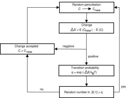
Figure 1: Logical scheme of the Metropolis algorithm.

The Metropolis algorithm Metropolis1953 was originally developped in 1952 to accurately simulate a group of atoms in equilibrium at a given temperature. The logical scheme of this algorithm is shown in figure 1. At each step of the iterative process, a random rearrangement of the configuration is made leading to a modification $\Delta E$ of the cost function. If the cost is lowered by this rearrangement $\Delta E\leq 0$, it is accepted and the next iterative step starts with the new configuration. If the rearrangement increases the cost $\Delta E>0$, it is not automatically rejected. Instead, a probability factor $q=\exp(-\Delta E/k_{B}T)$ constructed out of the cost modification $\Delta E$ is compared with a random number in the interval $[0,1]$. If the factor $q$ is greater than the random number, the new configuration is accepted, otherwise it is rejected. So, it becomes statistically more difficult for a rearranged configuration with $\Delta E>0$ to be accepted as the temperature $T$ decreases. This scheme can be applied directly to a cost function like (35).

Let us now state a number of important aspects to keep in mind when implementing an SA algorithm. (i) The initial temperature must be chosen with care. If one starts a simulation with the temperature set too high, the soliton may unwind. Also, the overall running time will be longer because of the increased number of cooling steps then needed. On the other hand, if the initial temperature is set too low, the system may stabilize in a local minimum when it is sufficiently cooled down. (ii) The cooling schedule must be smooth enough. It has been shown by Geman and Geman Geman that if the temperature decreases according to a logarithmic rule, the convergence to the global minimium of the system is guaranteed. However, faster cooling schemes can produce reliable results too. (iii) It is important that the initial guess for the field configuration possesses the winding number of the solution we seek. If it is not the case, the formation of isolated lumps of baryonic density is likely to occur as the simulation progresses. In our three dimensional simulations, we initialize the lattice with an appropiate degree rational map. (iv) The conservation of the baryonic number must be imposed explicitly in three dimensional simulations. This is done by adding a Lagrange multiplier to the action. This object tends to reject a trial configuration that compromises the quality of the topological integer, even if this configuration implies a lower value of the cost function. In the one dimensional case, this is not an issue since the conservation of the baryonic number is assured by the boundary conditions on the chiral angle $F(r)$.

The details concerning the sampling method we use and our criterion for the determination of thermal equilibrium will be discussed shortly.

V.2 One dimensional simulated annealing and rational maps

In our one dimensional approach, we first integrate out the angular dependence of the skyrmion using the rational maps ansatz. Then, SA finds the chiral angle $F(r)$ leading to a minimal value of the energy functional for generalized Skyrme models (25). To do this, we need a lattice that represents the radial degree of freedom $r$ in a discretized manner. In this context, the conservation of the topological integer $N$ is guaranted by the boundary conditions $F(0)=\pi$ and $F(\infty)=0$ and the degree $N$ of the rational map $R(z).$

To minimize the energy functional of a model, we need to compute $F(r)$ on the lattice. The energy and the baryonic number are evaluated halfway between two adjacent points of the lattice, $r_{i}$ and $r_{i+1}$. The value that the chiral angle and its derivative take there are given by

$$F(r_{i+1/2}) =\frac{F(r_{i})+F(r_{i+1})}{2}~{},$$ (36)

$$\frac{dF(r_{i+1/2})}{dr} =\frac{F(r_{i+1})-F(r_{i})}{dr}~{},$$ (37)

where $dr=r_{i+1}-r_{i}$. A cell represents the space between two adjacent lattice points. One assigns to each cell a value of energy and baryonic density as calculated at its center $r_{i+1/2}$.

SA relies on an iterative random process. To ensure that the sampling in space of field configurations is performed correctly, we must efficiently rearrange $F(r)$ during the simulation. We choose to perturbate randomly just one discrete value of $F(r)$ at each iteration, namely the one corresponding to the point $r_{i}$. Doing so, the energy and baryonic density of the two cells sharing the point $r_{i}$ are modified. This alteration of $F(r_{i})$ is then accepted or rejected according to the Metropolis algorithm. Explicitely, a random change of $F(r_{i})$ takes the form

$$F(r_{i})\longrightarrow F(r_{i})+A\cos(2\pi n),$$ (38)

where $A$ is the maximal amplitude of the change and $n$ is a random number in the interval $[0,1]$. An appropriate and efficient sampling will occur if $A$ is adjusted dynamically during the simulation so that $50\%$ of the new configurations are rejected. This strategy implies that $A$ decreases linearly with temperature $T$.

To implement an SA algorithm properly, thermal equilibrium must be reached at each temperature of the cooling scheme. The strategy we use is based on a statistical chain composed of a given number of iterations. The chain has a length set to 10 times the number of points on the lattice. This has the following statistical consequence. When the algorithm has done a number of random perturbations corresponding to the length of the chain, the value of $F(r)$ has been modified approximately 10 times at each point of the lattice. To state that thermal equilibrium is reached, we compare the lowest energy value encountered in the chain $E_{\mathrm{min}}$ and the sum of the energies obtained at each iteration of the chain $\sum_{\mathrm{tries}}E_{\mathrm{try}}$ to their equivalent in the previous chain. If these two values are higher in the present chain than in the previous, thermal equilibrium has been reached and the temperature may be lowered. In other words, another chain must be started at the same temperature as long as

• $E_{min}$ of the present chain $<$ $E_{min}$ of the previous chain or,

• $\sum_{\mathrm{tries}}E_{\mathrm{try}}$ of the present chain $<$ $\sum_{\mathrm{tries}}E_{\mathrm{try}}$ of the previous chain.

Figure 2: Temperature as a function of the cooling steps according to four different schemes. The curve which is distinct from the three others corresponds to a logarithmic scheme, i.e. of the form $T_{i}=0.95~{}T_{i-1}$. The other curves represent cooling schemes possessing the structure $T_{i}=T_{i-1}(X-i)/X$, where $X$ is fixed to $300$, $350$ and $400$, respectively from bottom to top.

Every time thermal equilibrium is achieved, the temperature is decreased according to a cooling schedule. In our one dimensional simulations, we use a logarithmic cooling because the computational cost is not an issue. This kind of schedule decreases the temperature by a fixed ratio at each step, for example $T_{i}=0.95~{}T_{i-1}$, presented on figure 2. In practice, faster cooling schemes can be used without negative impact on the quality of the global minimum obtained. Experience has shown that such a faster scheme can take the form $T_{i}=T_{i-1}(X-i)/X$, where $X$ is a constant factor, which still leads to reliable results. We have set the initial temperature to $T_{\mathrm{ini}}=1$ in all our one dimensional simulations. This value was obtained by trial and error while comparing the quality of the minimization.

To speed up the minimization process, we have even implemented an adaptive lattice. The simulation is started with a reasonably low number of points and a chiral angle which is a linear interpolation between $F(0)=\pi$ and $F(150)=0$. Typically, 100 points are used to cover the lattice that has 150 units of length $2\sqrt{2}/(eF_{\pi})$. When a global minimum is found, additional lattice points are added where the energy is concentrated and the temperature is set to its initial value $T_{\mathrm{ini}}=1$ before SA starts again. This procedure is repeated until the desired precision on the solution for $F(r)$ is achieved, corresponding to a lattice of approximately 650 points. However, this adaptive procedure is only practical in the one dimensional case, where the computational cost is relatively low. In three dimensional SA, computational time and computer memory considerations become important constraints. So, cooling the system several times to achieve the most convenient lattice spacing would not constitute an advantage in that case.

V.3 Three dimensional simulated annealing

The three dimensional SA algorithm is used to find exact solitonic solutions. This approach is a full field simulation where no constraints on the symmetries of the solution are imposed. Here are some important aspects of our three dimensional implementation.

The lattice we use is composed of $80\times 80\times 80$ points equally spaced by $0.12$ units of length $2\sqrt{2}/(eF_{\pi})$. This lattice spacing is somewhat large, but is a good compromise in regard to reducing the computational time. The cartesian axes go from $-4.8$ units to $4.8$ units in the $x$, $y$ and $z$ coordinates. This finite volume can cause undesirable numerical effects on the edge of the lattice. To significantly reduce these, we use a lattice with periodic boundaries. In this case the skyrmion interacts with itself over the boundaries, but its structure is not altered. The skyrmion only suffers a slight increase in energy.

Figure 3: Maximal amplitude $A$ of the random perturbations done on 3D field vectors as a function of temperature for the Skyrme model.

Because of topology, each lattice point is characterized by a four-component field $\phi_{m}$ which satisfies $\phi_{m}\phi_{m}=1$. As a consequence, perturbing the configuration by random rotations must also preserve the length of $\phi_{m}$, as explained in Hale2000 . These rotations are parametrized in terms of three random Euler angles. For computational purposes, we only consider small perturbations for one of the angles by limiting the random values to an upper bound $A$. Covering the whole solid angle is ensured by multiple rotations if needed. We adjust dynamically the parameter $A$ during the cooling process so that $60\%$ of the perturbations performed on the field $\phi_{m}$ are rejected. Starting with $T_{\mathrm{ini}}=0.02$ and using a cooling schedule of the form $T_{i}=T_{i-1}(300-i)/300$, where $i$ is a cooling step, the amplitude $A$ drops linearly with temperature (figure 3). This ensures that the rearrangements will not be too large as the temperature decreases, thus respecting the SA scheme.

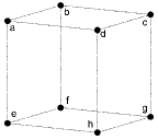
Figure 4: A cubic cell from the 3D lattice. This cell has a volume of $(0.12)^{3}$ units $(2\sqrt{2}/(eF_{\pi}))^{3}$. We identify its vertices with indices for further reference. The $x$, $y$ and $z$ axes are assigned in the directions of the segments $\overline{eh}$, $\overline{ef}$ and $\overline{ea}$ respectively.

To sample the fields on the lattice, we use again the concept of cell (figure 4). An iteration in the statistical chain starts with the random selection of a cell. Then, each of the eight vertices (lattice points) of the cell undergoes a rotation of the field. These rearrangements modify the energy and baryonic densities calculated at the center of the current cell and at the center of the 26 neibourghing cells, each of them having at least one lattice point in common with the randomly modified cell. We then use the Metropolis criterion to analyse the effect of the rotations on the energy of the 27 cells subsystem. If the acceptance criterion is confirmed, the changes affecting the eight lattice points are all accepted otherwise they are all rejected.

To compute the energy and baryonic densities at the center of a cell, one must rely on a linear interpolation using the value of the field at each of the eight vertices of the cell. Then, the energy density is evaluated at the center of the cell and the contribution to the total energy is obtained by mutiplying the density by the volume of the cell, $(0.12)^{3}$. Unfortunately, the linear interpolation does not preserve the relation $\phi_{m}\phi_{m}=1$, so we have to scale the fields following the interpolations. For example, the derivative at the center of a cell in the $x$ direction, refering to figure 4, is given by

$$\left.\frac{\partial\phi}{\partial x}\right|_{\text{~{}center}}=\frac{1}{0.12}~{}\left\{\text{Scaled}\left(\frac{1}{4}~{}[\phi(c)+\phi(d)+\phi(g)+\phi(h)]\right)-\text{Scaled}\left(\frac{1}{4}~{}[\phi(a)+\phi(b)+\phi(e)+\phi(f)]\right)\right\}~{}.$$

In our 3D simulations, we need to introduce a procedure to ensure that the baryonic number of the field configuration is conserved throughout the cooling process. A convenient way is to add a Lagrange multiplier to the action. This piece filters only appropriate random perturbations generated by the Metropolis algorithm. The Lagrange multiplier will tend to reject rearrangements compromising the quality of the calculated topological integer, regardless of their effect on the value of the energy functional being minimized. To help the convergence of SA towards the global minimium of the desired topological sector, we initialize the lattice with a field configuration that is already in the sector of interest. We use a rational map ansatz of adequate degree to generate an initial field configuration. In fact, the precise form of the initialization ansatz does not matter, as long as its degree $N=B$. For simplicity, we use the ansatz $R(z)=z^{N}$. Such a configuration possesses radial symmetry for $N=1$ and toroidal symmetry for $N>1$.

VI Numerical results and discussion

First, let us take a look at our results for the static energies and baryonic numbers presented in table 2. For the models considered in this work, we note that adding a positive (negative) weight $h_{m}$ leads to an increase (decrease) in the static energy of the skyrmion which depends on the size of $h_{m}$. For example, considering that $h_{4}$ is small compared to $h_{3}$, such a feature could explain the slight difference between the energies of the order-six and the order-eight models. Also, comparing the ratios $E_{N>1}/E_{1}$, multi-skyrmions solutions of extended models appear to be more stable than for the Skyrme model, for a greater part of their energy is used to create solitonic bound states. However, we cannot at this point confirm that these patterns are generic features and that they will hold for other extensions. Again, we recall that the results of the order-eight model should be taken with care, since the solutions are not global minima. The global minima which would lead to negative energy and a zero-size soliton is prevented by a finite lattice spacing. But the order-eight model and its solutions should be considered here as good approximations for more elaborate models such as (34) as can be seen from table 2.

	$\chi_{S}$ (Skyrme)			$\chi_{O6}$ (order 6)		$\chi_{O8}$ (order 8)		$\chi_{R}$ (all orders)
	RM	3D	3D Hale2000	RM	3D	RM	3D	RM	3D
$B_{1}$	0.9999	0.9974	1.0015	0.9999	0.9984	1.0000	0.9995	0.9999	0.9994
$E_{1}$	103.1306	103.091	104.45	129.9757	130.828	129.2987	130.242	129.3145	130.156
$B_{2}$	1.9999	1.9981	2.0030	2.0000	1.9995	2.0000	1.9998	—	1.9996
$E_{2}$	202.3558	198.139	199.17	253.2955	245.568	252.0314	244.542	—	244.609
$E_{2}/E_{1}$	1.9621	1.9219	1.9068	1.9488	1.8770	1.9492	1.8776	—	1.8793
$B_{3}$	3.0000	2.9981	3.0042	2.9999	2.9997	3.0000	2.9999	—	2.9998
$E_{3}$	297.5660	288.641	291.11	369.3230	354.405	367.7119	352.940	—	352.906
$E_{3}/E_{1}$	2.8853	2.7998	2.7870	2.8415	2.7089	2.8439	2.7099	—	2.7114
$B_{4}$	4.0001	3.9989	4.0048	3.9999	3.9997	4.0000	3.9997	—	3.9997
$E_{4}$	380.7257	377.281	375.50	467.3910	455.805	465.4414	454.205	—	454.190
$E_{4}/E_{1}$	3.6917	3.6597	3.5950	3.5960	3.4840	3.5997	3.4874	—	3.4895

Table 2: Results of SA in one dimension using the rational map ansatz (RM) and in three dimensions (3D) for the Skyrme model and extensions defined in (33, 34). For the Skyrme model the 3D results are compared with those of ref. Hale2000 . $B_{N}$ and $E_{N}$ are the computed baryonic number and energy for the soliton configuration with winding number $N$ respectively. The unit of energy is $F_{\pi}/(2\sqrt{2}e)$.

Figure 5: Chiral angles obtained with one dimensional SA for the Skyrme model and extensions of order six and order eight in the topological sector $B=1$. The lower curve corresponds to the $F(r)$ of the Skyrme model. The two higher-order extensions we have studied lead to superposed chiral angles decreasing slower that the one of the Skyrme model.

$\qquad\qquad B=1\qquad\qquad\qquad\qquad B=2\qquad\qquad\qquad\qquad\quad B=3\qquad\qquad\qquad\qquad B=4$

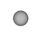
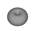
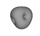
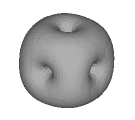
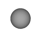
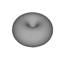
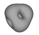
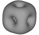
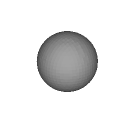
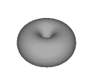
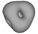
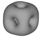
Figure 6: Plots of constant baryonic density ($0.0001$) obtained using three dimensional SA. From top to bottom are shown the results of the Skyrme model, the order-six extension and the order-eight extension.

The increase in the static energy of generalized skyrmions relative to those of the Skyrme model reflects itself in the structure of such solutions. The plots of constant baryonic density illustrated on figure 6 clearly show that extended skyrmions occupy a greater volume. This fact can also be supported by the rational maps approximation with one dimensional SA calculations (see the chiral angles in figure 5). The plots of figure 6 also strongly suggest that the symmetries of extended skyrmions are the same as those of the Skyrme model.

	Skyrme	Order 6	Order 8	Rational Model
$B=1$	$0.04$	$0.65$	$0.72$	$0.65$
$B=2$	$2.13$	$3.15$	$3.06$	—
$B=3$	$3.09$	$4.21$	$4.19$	—
$B=4$	$0.91$	$2.54$	$2.47$	—

Table 3: Differences in percent ($\%$) between the static energies of the solutions obtained using the rational maps ansatz and the ones obtained using three dimensional SA.

Let us now make quantitative remarks regarding the reliability of the rational maps ansatz. According to the conclusions of Houghton1998 , the rational maps ansatz should lead to computed static energies of $B>1$ for the original Skyrme model that are larger by a few percent compared to the exact solutions. Indeed, using the data of table 2, we see that this is true for the Skyrme model, as well as for the two extensions we have considered. The differences between the two approaches are reported in table 3. It seems that adding new terms to the Skyrme model slightly compromises the reliability of the rational maps ansatz. However, the discrepancies are quite moderate and the rational maps approximation remain valid for extensions of the Skyrme model. Therefore, both baryonic density plots and the comparison with rational map ansatz indicate that the solutions of the Skyrme model and those of the generalized models we have studied are characterized by a similar angular distribution, i.e. the same symmetries.

Even if SA leads to satisfying soliton solutions, some numerical features that are inherent to the simulation occur and it is important to review their effects on our results. First of all, we note that despite what we expected, the static energies of the $B=1$ solitons in the 1D and 3D schemes do not exactly coincide. This is mostly due to a larger spacing of the 3D lattice, which must be imposed in regard to computational time and memory. Moreover, the finite volume of the 3D (periodic) lattice induces an error estimated at $1\%$  Hale2000 , because the soliton interacts with itself over the boundaries. Another source of error is due the non logarithmic nature of our cooling schedule which amounts to about $0.1\%$. Finally, an error of the order of $0.3\%$ is expected to arise as a result of the way we evaluate the derivatives on the finite spacing lattice.

For the sake of completeness, we now compare our 3D results (table 2) with existing calculations. For the Skyrme model, previous calculations that were performed using several approaches, for example an axially symmetric ansatz Bratten1988 ; Kopeliovich1987 , a relaxation method Bratten1990 ; Battye19971 ; Battye19972 and more recently SA Hale2000 are in accord with the results presented in this work. Kopeliovich and Stern Kopeliovich1987 and Floratos et al. Floratos2001 have also analyzed some Skyrme model extensions up to order six but the choice of weights $h_{3}$ and $h_{4}$ are different so our model cannot be compared directly. However, their solutions exhibit the same symmetries as in figure 6. The remaining results of table 2 are completely new.

Even if the results that we have obtained so far support the rational map conjecture proposed in this work, its general character needs to be investigated in greater detail. There are indeed indications that a simple modification to the Lagrangian may change the form of the soliton, e.g. adding a mass term Battye2004 . As a starting point, one could analyze other extended models obeying the positivity constraints presented in section IV. The SA algorithm is particurlarly well suited to this kind of problem since there is no need to handle complex differential equations. It could also be interesting to add a pion mass term or to study models having different structures, for example a contribution coming from the rotational energy of the skyrmion. In fact, the versatility of the SA algorithm makes it possible to study a large variety of models. Some investigations along these paths are already under way.

References

- (1) T. H. R. Skyrme, Proc. Roy. Soc. Lond. A260, 127 (1961).
- (2) G. ’t Hooft, Nucl. Phys. B72, 461 (1974).
- (3) E. Witten, Nucl. Phys. B160, 57 (1979).
- (4) A. Jackson, A. D. Jackson, A. S. Goldhaber, G. E. Brown, and L. C. Castillejo, Phys. Lett. B154, 101 (1985).
- (5) L. Marleau, Phys. Lett. B235, 141 (1990).
- (6) S. Dubé, L. Marleau, Phys. Rev. D41, 1606 (1991).
- (7) A. D. Jackson, C. Weiss, and A. Wirzba, Nucl. Phys. A529, 741 (1991).
- (8) G. S. Adkins, C. R. Nappi, and E. Witten, Nucl. Phys. B228, 552 (1983).
- (9) V.B. Kopeliovich and B.E. Stern, Zh. EKsp. Teor. Fiz. 45. 165 (1987); JETP Lett. 45,203 (1987).
- (10) E. Braaten and L. Carson, Phys. Rev. D38, 3525 (1988).
- (11) E. Braaten, S. Townsend, and L. Carson, Phys. Lett. B235, 147 (1990).
- (12) R. A. Battye, P. M. Sutcliffe, Phys. Rev. Lett. 79, 363 (1997).
- (13) R. A. Battye, P. M. Sutcliffe, Phys. Lett. B391, 150 (1997).
- (14) I. Floratos, B. Piette, Phys. Rev. D64, 045009 (2001).
- (15) M. Hale, O. Schwindt, and T. Weidig, Phys. Rev. E62, 4333 (2000).
- (16) S. Kirkpatrick, C. D. Gellat, and M. P Vecchi, Science 220, 671 (1983).
- (17) N. Metropolis, A. W. Rosenbluth, M. N. Rosenbluth, and A. H. Teller, J. Chem. Phys. 21, 1087 (1953).
- (18) C. J. Houghton, N. S. Manton, and P. M Sutcliffe, Nucl. Phys. B510, 507 (1998).
- (19) R. A. Battye, P. M. Sutcliffe, Phys. Rev. Lett. 86, 3989 (2001).
- (20) L. Marleau, J.F. Rivard, Phys. Rev. D63, 036007 (2001).
- (21) N.S. Manton, Commun. Math. Phys. 111, 469 (1987).
- (22) R. A. Battye, P. M. Sutcliffe, Rev. Math. Phys. 14, 29 (2002).
- (23) R. A. Battye, P. M. Sutcliffe, Nucl. Phys. B705, 384 (2005)
- (24) S.Geman, D.Geman, IEEE Trans. Pattern. Anal. Mach. Intell. 26, 721 (1984).