Strings with a confining core in a Quark-Gluon Plasma

Abstract

We consider the intersection of N different interfaces interpolating between different $Z_{N}$ vacua of an SU(N) gauge theory using the Polyakov loop order parameter. Topological arguments show that at such a string-like junction, the order parameter should vanish, implying that the core of this string (i.e. the junction region of all the interfaces) is in the confining phase. Using the effective potential for the Polyakov loop proposed by Pisarski for QCD, we use numerical minimization technique and estimate the energy per unit length of the core of this string to be about 2.7 GeV/fm at a temperature about twice the critical temperature. For the parameters used, the interface tension is obtained to be about 7 GeV/fm². Lattice simulation of pure gauge theories should be able to investigate properties of these strings. For QCD with quarks, it has been discussed in the literature that this $Z_{N}$ symmetry may still be meaningful, with quark contributions leading to explicit breaking of this $Z_{N}$ symmetry. With this interpretation, such QGP strings may play important role in the evolution of the quark-gluon plasma phase and in the dynamics of quark-hadron transition.

Key words: quark-hadron transition, relativistic heavy-ion collisions, early universe, strings

I Introduction

Physics of quark-gluon plasma (QGP) and the quark-hadron phase transition has become a very active area of research in recent years. There are several reasons for this. The most important motivation comes from the ongoing, and upcoming, relativistic heavy-ion collision experiments where it is widely believed that a hot dense region of QGP will be created. This will provide the opportunity for a controlled study of high temperature phase of a theory as rich as QCD, as well as the dynamics of phase transition in a relativistic quantum field theory. Such studies are especially important for the early universe where the universe was in the QGP phase until it was about few microseconds old. Many studies have been carried out about possible observational implications of the quark-hadron phase transition in the early universe. Further, lattice results have given a control on the understanding from the theory side and the stage is set for confronting observations with lattice results for deeply non-perturbative regime of the quark-hadron phase transition.

This richness of QCD is manifested in non-trivial phases and structures allowed by the theory in various regimes of temperature, chemical potential, and other control parameters (some of which may be primarily of theoretical importance, such as quark masses). Even the perturbative regime of high temperature QGP phase has non-trivial vacuum structure as seen by using the expectation value of the Polyakov loop $l(x)$ as the order parameter for the confinement-deconfinement phase transition [1]. This order parameter transforms non-trivially under the center $Z(3)$ of the color SU(3) group and is non-zero above the critical temperature $T_{c}$. This breaks the global $Z(3)$ symmetry spontaneously above $T_{c}$, while the symmetry is restored below $T_{c}$ in the confining phase where this order parameter vanishes.

In the QGP phase, due to spontaneous breaking of the discrete $Z(3)$ symmetry, one gets domain walls (interfaces) which interpolate between different $Z(3)$ vacua. The properties and physical consequences of these $Z(3)$ interfaces have been discussed in the literature [2]. (Though, we mention that it has also been suggested that these interfaces should not be taken as physical objects in the Minkowski space [3]. Similarly, it has also been subject of discussion whether it makes sense to talk about this $Z(3)$ symmetry in the presence of quarks [4].) The presence of quarks can be interpreted as leading to explicit breaking of $Z(3)$ symmetry, lifting the degeneracy of different $Z(3)$ vacua [5, 6, 7]. In this approach, with quarks, $Z(3)$ interfaces become unstable and move away from the region with the unique true vacuum. We will take this interpretation to be valid for the case with quarks. Though our main discussion will be for the pure gauge theory which we discuss first. Later we will comment on the situation with quarks.

We will consider specific configurations of $Z(3)$ interfaces, namely the intersection of all three different interfaces in the high temperature deconfining phase. (For general SU(N) case one will consider the intersection of N different $Z(N)$ interfaces.) Topological arguments then show that at the line-like intersection of these interfaces, the order parameter $l(x)$ should vanish. This leads to a topological string configuration with core of the string being in the confining phase. It is important to note that such a string has exactly reverse physical behavior compared to the standard QCD string. The QCD string exists in the confining phase, connecting quarks and antiquarks, or forming baryons, glueballs etc. Inside the QCD string energy density is high enough, and distance scales small enough, that the core region behaves as a deconfined region. In contrast the string we are discussing exists in the high temperature deconfined phase. Its core is characterized by restored $Z(3)$ symmetry, implying that it is in the confined phase. To differentiate it with the standard QCD string, we call this string configuration the QGP string. It is also important to note that although the standard QCD string breaks by creating quark-antiquark pairs, the QGP string cannot break as it originates from topological arguments. This QGP string, thus should either form closed loops, or it should end at the boundary separating the deconfined phase from the confined phase.

To estimate the physical properties of such a string configuration for QCD, we use the effective potential proposed by Pisarski [6, 7] (see, also ref. [8]) for the Polyakov loop $l(x)$. Using this Polyakov loop model, we estimate the energy per unit length of the QGP string to be about 2.7 GeV/fm at a temperature about $2T_{c}$. The interface tension is found to be about 7 GeV/fm² at this temperature.

It is clear that the structure of this QGP string is similar to the standard axionic string which forms at the junction of axionic domain walls [9]. The consequences of the QGP string therefore can be determined following those discussions. Presence of quarks can then be taken in terms of explicit $Z(3)$ symmetry breaking. This will lead to decay of $Z(3)$ interfaces along with rapid decay of the associated strings. One important difference with the axionic strings is that the axionic strings are supposed to be produced at the Pecci-Quinn symmetry breaking transition, with symmetry broken in the low temperature phase. Thus the standard picture of string formation in a phase transition is applicable. In contrast, for the QGP strings, symmetry is always broken in the high temperature phase, it gets restored below $T_{c}$, the QCD transition temperature. The formation of these QGP strings thus will be of a different nature. Further, this string network will melt away below $T_{c}$. Another difference between the present case and the standard axionic models is that, as we will see below, for the axionic models the central bump in the effective potential is higher than the barrier between different $Z(N)$ vacua. In those axionic models, one can therefore restrict the order parameter $|\phi|\sim\phi_{0}$, where $\phi_{0}$ is approximately the value of the order parameter corresponding to the absolute minimum of the effective potential. This reduces the problem effectively to that for a scalar field with a disconnected vacuum manifold. The solution for kink solitons are well known in such models. In contrast, for the present case the situation is reversed. Here the barrier between different $Z(N)$ vacua is much higher than the central bump. Thus, here the problem cannot be reduced to that of the standard scalar kink soliton and as we will explain, the discussion of appropriate domain wall solution becomes much more involved.

Presence of such strings should have strong effects on the properties of the QGP phase as well as on the dynamics of the quark-hadron phase transition. With pre-existing string network with confining core, the transition to the confining phase should begin from regions near the string. This is certainly true for a first order transition, where the string network will make heterogeneous nucleation, with bubbles of confining phase forming at these QGP strings, more dominant compared to the conventional homogeneous nucleation. Even for a second order transition, the transition may not remain uniform, and may proceed from the strings outward. We hope to discuss the effects of such a modified picture of phase transition on baryon inhomogeneity generation for the early universe as well as for relativistic heavy ion collision experiments in a future work.

The paper is organized in the following manner. In section II, we briefly review the Polyakov loop model of Pisarski and discuss the topological arguments leading to the existence of the QGP string. In section III, we discuss the numerical technique and the properties of the $Z(3)$ interface. Section IV discusses junctions of these interfaces, i.e. the profile of the QGP string. We also comment here on the effect of quarks on these solutions. Section V presents conclusions.

We mention here that the string-like junction of these $Z(N)$ interfaces for an SU(N) theory has been discussed in ref.[10], but with a completely different interpretation [10]. In ref.[10] these intersections are identified with the space-like world lines of color magnetic monopoles in the context of confinement by monopole condensation.

II The Polyakov loop model

As we mentioned above, we will focus on pure SU(N) gauge theory and later discuss the case with quarks. In this case, an order parameter for the confinement-deconfinement phase transition is the Polyakov loop $l(x)$ which is defined as,

$$l(x)=\frac{1}{N}tr\Bigl{(}Pexp\Bigl{(}ig\int^{\beta}_{0}A_{0}(x,\tau)d\tau\Bigr{)}\Bigr{)}.$$ (1)

Here $P$ denotes path ordering, $g$ is the gauge coupling, $\beta=1/T$, with $T$ being the temperature, $A_{0}(x,\tau)$ is the time component of the vector potential at spatial position $x$ and Euclidean time $\tau$. $l(x)$ is thus a complex scalar field. Under a global $Z(N)$ symmetry transformation, $l(x)$ transforms as,

$$l(x)\rightarrow exp\bigl{(}\frac{2\pi in}{N}\bigr{)}l(x),~{}~{}n=0,1,..(N-1).$$ (2)

For temperatures above the critical temperature $T_{c}$, in the deconfining phase, the expectation value of the Polyakov loop $l_{0}=<l(x)>$ is non-zero corresponding to the finite free energy of isolated test quarks. This breaks the $Z(N)$ symmetry spontaneously. At temperatures below $T_{c}$, in the confining phase, $l_{0}$ vanishes, thereby restoring the $Z(N)$ symmetry [1]. We now restrict to the case of QCD with $N=3$ and take the effective theory for the Polyakov loop as proposed by Pisarski (see ref. [6, 7] for details), given by the following effective Lagrangian density,

$$L=\frac{N}{g^{2}}|\partial_{\mu}l|^{2}T^{2}-V(l).$$ (3)

Here, $N=3$ and $V(l)$ is the effective potential for the Polyakov loop given by,

$$V(l)=\Bigl{(}-\frac{b_{2}}{2}|l|^{2}-\frac{b_{3}}{6}\bigl{(}l^{3}+(l^{*})^{3}\bigr{)}+\frac{1}{4}\bigl{(}|l|^{2}\bigr{)}^{2}\Bigr{)}b_{4}T^{4}.$$ (4)

$l_{0}$ is then given by the absolute minimum of $V(l)$. Normalization of $l(x)$ is chosen such that $l_{0}\rightarrow 1$ as $T\rightarrow\infty$. Values of various parameters in Eqs.(3),(4) are fixed in ref.[7] by making correspondence to lattice results. We make the same choices, and give those values below.

The values of various parameters in Eq.(4) are fixed to reproduce lattice results [11] for pressure and energy density of pure SU(3) gauge theory. For pure gauge theory we will use the same parametrization as is chosen in ref.[12] where the coefficient $b_{3}$ and $b_{4}$ has been taken as, $b_{3}=2$ and $b_{4}=0.6061$. We will take the same value of $b_{2}$ for real QCD (with three massless quark flavors), while the value of $b_{4}$ will be rescaled by a factor of $47.5/16$ to account for the extra degrees of freedom relative to the degrees of freedom of pure gauge theory, as in ref.[12]. The temperature dependent coefficient $b_{2}(T)$ has been taken from ref.[12, 7] which is expressed in terms of the ratio $r$ ($=T/T_{c}$) as, $b_{2}(r)=(1-1.11/r)(1+0.265/r)^{2}(1+0.300/r)^{3}-0.487$. With the coefficients chosen as above, the expectation value of the order parameter approaches to $x=b_{3}/2+\frac{1}{2}\sqrt{b_{3}^{2}+4~{}b_{2}(T=\infty)}$ for temperature $T\rightarrow\infty.$ As in ref.[7], we will use the normalization such that the expectation value of the order parameter $l_{0}$ goes to unity for temperature $T\rightarrow\infty$, hence the fields and the coefficients are rescaled as $l\rightarrow l/x,b_{2}(T)\rightarrow b_{2}(T)/x^{2},b_{3}\rightarrow b_{3}/x$ and $b_{4}\rightarrow b_{4}~{}x^{4}$ to ensure proper normalization of $l_{0}$.

By writing $l=|l|e^{i\theta}$ we see that the $b_{3}$ term in Eq.(4) gives a $cos(3\theta)$ term, leading to $Z(3)$ degenerate vacua for non-zero values of $l$, that is for $T>T_{c}$. With the choice of parameters as above, the value of $T_{c}$ is $\sim 182$ MeV. The $Z(3)$ interface solution will correspond to a planar solution (say in the x-y plane) where $l$ starts at one of the minimum of $V(l)$ at $z=-\infty$ and ends up at the other minimum of $V(l)$ at $z=+\infty$. These $Z(3)$ interfaces have been extensively discussed in the literature [2].

Consider now the junction of all three different $Z(3)$ interfaces, say with the line like junction being along the z axis. The interfaces then will be perpendicular to the x-y plane. It is immediately clear that as one considers a closed loop in the physical space encircling the z axis, then one encircles $l=0$ point in the complex $l$ plane. It is then obvious from the continuity of $l$ that $l$ must vanish along the z axis. This is the standard argument for topological string solutions (more specifically axionic strings, though situation here is somewhat different due to large barrier height, as discussed below). These are topological strings and hence cannot break. Note that, in contrast the standard QCD string can break by creating quark-antiquark pairs.

The potential given in Eq.(4), leads to a weak first order transition. We show the plot of $V(l)$ in $\theta=0$ direction in Fig.1a for a value of temperature $T=185$ MeV. This shows the metastable vacuum at $l=0$. To see the $Z(3)$ structure of the vacuum we plot the potential $V(l)$ as a function of $\theta$ for fixed $|l|=l_{0}$, where $l_{0}$ corresponds to the absolute minimum of $V(l)$. This is shown in Fig.1b. An important thing to note from Fig.1a,b, is that the height of the barrier between different $Z(3)$ vacua is much higher than the height of the barrier between the metastable vacuum at $l=0$ and the true vacuum. This situation is in complete contrast to the standard axionic models where the central bump is higher than the barrier between different $Z(N)$ vacua. In those axionic models, one can therefore restrict $|l|\sim\l_{0}$ which reduces the problem effectively to that with a scalar field with a disconnected vacuum manifold. The solution for kink solitons are well known in such models.

Such a solution cannot be found here, as the height of barrier between the $Z(3)$ vacua is much higher than the central bump. At high temperatures the ratio of the heights of the $Z(3)$ barrier and the central bump reduces, but it still remains much larger than 1. In Fig.2a we show the surface plot of the potential $V(l)$ in Eq.(4) in the complex $l$ plane for $T=400MeV$. Plot range in the $V$ axis is restricted to make the $Z(3)$ barriers and the central bump distinctly visible. To compare this situation with a standard axionic model case (with same $Z(3)$ symmetry), we show in Fig. 2b the potential in Eq.(4) with the coefficient $b_{2}$ multiplied by 100. This raises the central bump higher than the $Z(3)$ barriers. For a potential like in Fig.2b the $Z(3)$ domain wall solution is physically clear as the order parameter interpolates between the different $Z(3)$ vacua through the (smaller) barrier in the valley. In contrast, in Fig.2a, the lowest potential energy path from one $Z(3)$ vacuum to another goes through the origin $l=0$. It may give the impression that the $Z(3)$ interface will have $l=0$ in the middle of the interface. If that was true then it will imply that these $Z(3)$ interfaces have confining regions in the middle, which will not be in agreement with other studies of $Z(3)$ interfaces for QCD [2]. However, as we will discuss in the next section, the actual domain wall, which is a solution of the field equations, cannot have $l=0$ inside it. Still, a potential like in Fig.2a, makes it impossible to reduce the Lagrangian of Eq.(3) to an effective Lagrangian with kink solutions (as in the case of axionic models), and one has to find numerical techniques to determine the appropriate interface solution. We discuss this in the next section.

III Numerical techniques and the $Z(3)$ interface profile

First let us see general properties of the interface solution for the effective potential shown in Fig.2a. We are interested in time independent solutions. (This is in the absence of quarks. With quarks, $Z(3)$ symmetry will be explicitly broken, so there will not be any time independent interface or string solutions.) For a planar wall in the x-y plane we can write down the field equation as

$$\frac{d^{2}l_{i}}{dz^{2}}=\frac{g^{2}}{NT^{2}}\frac{\partial V(l_{1},l_{2})}{\partial l_{i}},$$ (5)

where we have written $l=l_{1}+il_{2}$. Using generalization of standard techniques [13], we interpret $z$ as time, and $l_{1}$ and $l_{2}$ as the two dimensional position space for a particle which is moving under the influence of potential = $-V(l_{1},l_{2})(\frac{g^{2}}{NT^{2}})$. Domain wall solution will then correspond to the particle trajectory which for $z\rightarrow-\infty$ approaches one of the minima of $V(l)$, while for $z\rightarrow+\infty$ it approaches a different minima of $V(l)$.

Fig.3 shows the plot of the inverted potential, i.e. $-V(l_{1},l_{2})$. Minima of $V$ now become maxima of $-V$. Again, to show the shape of the potential clearly, we have restricted the range of plot for negative values. As we mentioned above, the domain wall solution will correspond to the particle trajectory starting at the top of one of the hills, say, at $P$, and ending at the top of another hill, say at $Q$. With this picture it becomes immediately obvious that the domain wall solution cannot go through $l=0$. The particle starting at $P$, and rolling down to $l=0$ cannot turn back to end up at $Q$. It will rather go to the other side and roll away downward, as shown by the dashed curve in Fig.3. To end up at $Q$, the trajectory must loop back before reaching $l=0$, as shown by the solid curve in Fig.3. Thus, $l$ must remain non-zero inside the domain wall.

What we have described above is a simple generalization of the basic idea of how domain wall solution is found for a real scalar field. For real scalar field, one can numerically determine the solution of the field equation by tuning up the initial starting point of the particle (i.e. the field value), depending on whether the solution overshoots, or undershoots at large time (i.e. large $z$) [13]. However, for complex $l$, this tuning up of the initial condition becomes very difficult to determine depending on the nature of large time (large $z$) behavior of the solution. One will need to tune up both components $l_{1}$ and $l_{2}$ appropriately, depending on the details of large $z$ behavior, and it becomes very difficult to develop suitable criterion for this. This is certainly an interesting problem to develop suitable numerical scheme for numerically solving the differential equations to determine the domain wall solution for this type of potential.

In the absence of such a technique to determine the solution of the differential equation, we resort to numerical minimization of the energy to determine the appropriate solutions. Such a method is in general difficult to implement as one needs to be reasonably certain that one has not found a local minimum of the energy functional. The only way is to try different initial configurations with varying lattice sizes, and variational parameters, and see whether one gets the same final configuration. We have carried out such tests in our numerical minimization and we believe our results are trustworthy from this point of view.

For time independent case, the energy density from Eq.(3),(4) is,

$${\cal E}=\frac{NT^{2}}{g^{2}}|\bigtriangledown l|^{2}+V(l).$$ (6)

For the planar domain wall solution (say in x-y plane), this energy density is integrated along the z axis to get the energy per unit area $E_{W}$ of the wall. For string solution along z axis (discussed in the next section), this energy density is integrated in the x-y plane to get the energy per unit length $E_{S}$ of the string. Numerical minimization of $E_{W}$ (and $E_{S}$ respectively) is carried out as described below.

For the energy minimization, we have used a code as was used in ref.[14]. To determine the domain wall solution we only need to consider the profile of $l$ in one dimension (along $z$), so we restrict the two dimensional simulation of ref.[14] to one dimension. We fix the values of $l$ at the two boundaries of the one dimensional lattice as $l=l_{01}$ and $l=l_{02}$ where $l_{01}$ and $l_{02}$ are the values of $l$ corresponding to the two distinct minima of $V(l)$. For the intermediate lattice points we use an interpolating configuration between these two values. For small physical size of the lattice we use linear interpolation from one boundary to the other boundary, while for a large physical size of the lattice (compared to wall thickness) we use linear interpolation in a smaller, central portion of the lattice. In both situations we get the same final configuration for the interface. (If we use linear interpolation for the entire large lattice also then the minimization program gets trapped in some local minimum of energy converging to a configuration which has much larger energy.) We use a large lattice with 10⁴ points, with lattice spacing being 0.002 fm. The physical size of the one-dimensional lattice is then 20 fm. In this case we used linear interpolation for the middle 10 fm portion of the lattice for the initial configuration. Field configuration is then fluctuated at each lattice point, while fixing the boundary points, and energy is minimized. The configuration with the lowest value of energy is finally accepted (when the energy almost settles down to a definite value) as the correct profile of the interface and corresponding energy is taken as the energy (per unit area) of the domain wall. In the following we explain the essential aspects of this energy minimization technique [14].

We have used over relaxation technique for energy minimization, as in ref.[14], which we have found to be very efficient for our case. This consists in first determining the most favorable fluctuation in the field at a given site by fluctuating field there and considering the change in the energy density. The most suitable fluctuation corresponds to the minimum of the parabola which passes through these values of energy densities (corresponding to fluctuated values of the field). Then the actual change in the field is taken to be larger (by a certain factor) than this most suitable fluctuation. We have found that changing this factor in the range of 0.01 - 0.03 worked best for our case.

The minimization code has been tested with two dimensional lattice for finding the configuration of a standard U(1) global string, with a complex scalar order parameter $\phi$ [14]. Initial configuration of $\phi$ is chosen to be a winding number one, azimuthally symmetric configuration with some initial function for $|\phi(r)|$. We then minimize the energy and determine $\phi(r)$ which gives the lowest energy configuration. It is found that even if the initial profiles for $\phi(r)$ prescribed are very different (for example we have tried out triangular form for $\phi(r)$) , after about 200 iterations, $\phi(r)$ converges to the exact solution as obtained by numerically solving the field equations using a Runge- Kutta algorithm of fourth order accuracy.

Fig.4 shows the profile for the domain wall solution for $T=400MeV$. The surface tension of the wall in this case is found to be about 7 GeV/fm². Note that $l$ remains non-zero in the profile of the wall, as we argued above. As $T$ approaches $T_{c}$, the heights of the barriers between different $Z(3)$ vacua become much higher compared to the central bump (in Fig.2a). In such a situation, as one can see from Fig.3, in order to end up at Q, starting from P, the particle trajectory will have to loop back from a point which gets closer to the origin. This is indeed what we see in our numerical simulation also. We find that as $T$ approaches $T_{c}$, the value of $l$ in the middle of the domain wall profile becomes very small, but it always remains non-zero. We use $T=400$ MeV to get the profile of the domain wall (and the QGP string) to show distinctly non-zero $l$ profile for the wall. We mention here that, as mentioned in ref. [7], the parameter values used here are not valid for high temperatures. Our purpose here is not to be very precise about the numbers we get but about the qualitative aspects of the solutions we get. Also, the energies etc. we get may be correct up to factors of order unity.

IV Junctions of $Z(3)$ interfaces, the string profile

We now consider a configuration which corresponds to the junction of three different $Z(3)$ interfaces. As we discussed above, by considering a closed loop in the physical space encircling this junction, we see that the order parameter encircles $l=0$ point in the complex $l$ plane. From the continuity of $l$, it then follows that $l$ must vanish along the line forming the junction of the interfaces. This, therefore, leads to a topological string configuration whose core is in the confining phase.

To determine the profile of this QGP string, we use the numerical minimization as described in the previous section, with a two dimensional lattice. We have used a 600 $\times$ 600 lattice, with lattice spacing being 0.01 fm. The physical size of the lattice is then 6 fm $\times$ 6 fm. The string is taken to be perpendicular to the lattice, with the lattice giving a cross-section of the string, as well as the interfaces attached to it. We start with a trial configuration which has isotropic variation of $\theta$ (as appropriate for the conventional U(1) string), with the magnitude of $l$ vanishing at the center of the lattice. For the trial configuration we take the radial profile of $|l|$ such that it is zero at the center of the lattice and increases to the vacuum value of $l$ exponentially with a typical distance scale of few fm. We know that for the $Z(3)$ string, $\theta$ variation will not remain isotropic, it will become concentrated in the three domain walls whose junction will be the string. Thus we cannot fix the field at the boundary of the two dimensional lattice during minimization procedure. If we do not fix field anywhere and carry out the minimization, then string leaves the lattice due to asymmetric interface lengths (for a square lattice which we use). To handle this problem, we fix the center of the string [14]. The center of the string (where $l=0$) is chosen to lie at the middle of an elementary lattice square. We then fix $l$ at the four lattice points forming this particular lattice square. Everywhere else $l$ is fluctuated, and the energy is minimized to get lowest energy string profile. Since $l$ is fixed only for a very tiny elementary square (with lattice step being 0.01 fm), it causes negligible error in the determination of the correct string profile and string energy.

Fig.5 shows the surface plot of $-l$ showing clearly the string, connected to three interfaces. We thus see that despite very different barrier ratios for the potential in Eq.(4) and the standard axionic case (as shown in Fig.2a,2b), the string configuration is very similar to the standard axionic string connected to the $Z(3)$ interfaces. Determination of the energy of the string in this case becomes ambiguous due to the contribution of the energy of the interfaces. To separate out the string core energy contribution we use the following method. For the two dimensional cross-section of string profile, we obtain the net energy $E(r)$ within radius $r$ starting from the center of the string by integrating ${\cal E}$ in Eq.(6) for the configuration of Fig.5 inside a circle of radius $r$, with the center of the circle being at the center of the string. $E(r)$ will get contribution from the core of the string initially, but for large $r$ the contribution of interface energy will dominate. We can then parametrize $E(r)$ as follows,

$$E(r)=E_{0}(r),~{}~{}~{}0<r<r_{0}$$ (7)

$$E(r)=E_{0}(r_{0})+3\sigma(r-r_{0}),~{}~{}~{}r>r_{0}$$ (8)

Here, $E_{0}(r)$ denotes the core energy contribution which should be the dominant contribution up to some distance $r_{0}$. Beyond $r_{0}$, the linear contribution of interfaces becomes significant. By plotting $E(r)$ vs. $r$, we can get $\sigma$ as well as the core energy $E_{0}(r_{0})$. Fig.6 shows this plot. We have fitted the large $r$ part of the plot with a straight line. Its slope is found to be about 23 GeV/fm², giving the value of $\sigma\simeq 7.7$ GeV/fm² in reasonably good agreement with our numerical estimate for the wall tension given in the previous section. The core energy $E_{0}(r_{0})$ is found to be about 2.7 GeV/fm.

Let us now come back to the issue of quarks and the $Z(3)$ symmetry. The effect of quarks on this $Z(3)$ symmetry and $Z(3)$ interfaces etc. has been discussed in detail in the literature [4, 5]. It has been suggested that in the presence of quarks, the $Z(3)$ symmetry becomes meaningless, and there is no sense in talking about $Z(3)$ interfaces etc. [4]. It has also been advocated in many papers, that one can take the effect of quarks in terms of explicit breaking of $Z(3)$ symmetry [5, 6, 7]. In such a case, the interfaces will survive, though they do not remain solutions of time independent equations of motion. It has been argued in ref.[7] that the effects of quarks in terms of explicit symmetry breaking may be small, and the pure glue Polyakov model may be a good approximation. We will therefore assume that the effects of quarks is either negligible, or it just contributes explicit symmetry breaking terms which can make the interface and the string solution time dependent, but not invalid.

With the explicit symmetry breaking, the interfaces and string will develop dynamics, for example, the interfaces will start moving away from the direction where true vacuum exists. The string will also not have three interfaces forming symmetrically around it, and hence will start moving in some direction. Such motions may cause important differences on long time behavior (as for the axionic strings), but for short time it may be immaterial. This is because strings and domain walls anyway move around after formation due to the fact that they have large tensions and at the time of formation they almost never form in symmetric configurations. Thus the initial time dynamics of these $Z(3)$ interfaces and QGP string may not be much distinct from the case when there is no explicit $Z(3)$ symmetry breaking. This should be the situation appropriate for relativistic heavy-ion collisions. Of course the issue of initial time here is subtle as the strings exist in the high temperature phase, compared to the standard axionic strings which exist in the low temperature phase. Effects of these strings and their properties for pure gauge theories could be investigated by lattice simulations. As elaborated above, these strings, which are embedded in the QGP phase, have confining core. Because of this these strings can affect the dynamics of quark-hadron phase transition in important ways. It is possible that, as the transition temperature is approached from above, string cores may swell, and trigger the transition process. For a first order transition, the string with its confining core will act as an ideal site for bubble nucleation. This type of situation is often seen in condensed matter systems. For example in a nematic liquid crystal system when the system is heated back to the isotropic phase, with strings existing in the nematic phase, bubbles of isotropic phase nucleate primarily on top of the string defects. Same thing should happen here also. As the confining core exists inside the QGP strings, nucleation of a bubble on top of strings requires smaller free energy barrier to be overcome by thermal fluctuations. We thus expect that instead of homogeneous nucleation of bubbles one should get bubble nucleation happening on top of the entire QGP string network. We hope to investigate some of these possibilities in a future work.

V conclusions

We have discussed special configurations of junctions of $Z(N)$ interfaces for an SU(N) gauge theory and have shown that these correspond to topological strings which have confining phase in the core. Using the Polyakov loop model of Pisarski [6] for QCD, we have estimated the energy of this QGP string to be about 2.7 GeV/fm for a temperature about $2T_{c}$. Lattice simulation of pure gauge theories should be able to investigate properties of these strings. With the interpretation that quark contributions lead to explicit breaking of this $Z_{N}$ symmetry [5, 6, 7], such QGP strings may play important role in the evolution of the quark-gluon plasma phase and in the dynamics of quark-hadron transition.

As these strings exist in the high temperature phase (the $Z(3)$ symmetry being restored at low temperatures), formation and evolution of these strings will have unconventional features. The dynamics of a first order quark-hadron transition for a QGP region infested with these QGP strings with confining cores may be very different from the conventional scenarios. Even for a second order transition, due to large inhomogeneities present in the form of this string network, it is possible that the transition may proceed from the strings outward. It will be interesting to investigate if baryon inhomogeneities can be generated in this way even if the transition is of second order (or a cross-over). We hope to address these issues in a future work.

ACKNOWLEDGEMENTS

We are very thankful to Sanatan Digal, Rajarshi Ray, Supratim Sengupta, Soma Sanyal, Balram Rai, V. Sunil Kumar, and V.K. Tiwari for useful discussions and comments. We especially thank Amit Kundu, B.K. Patra, and Aporva Patel for early discussions on this subject.

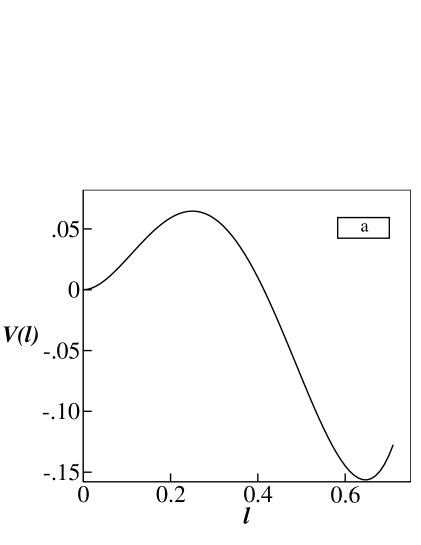
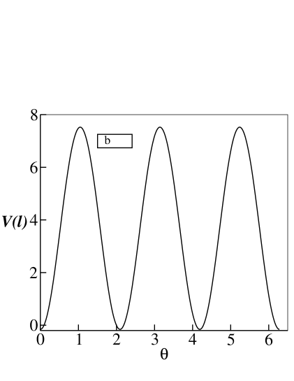
FIG. 1.:

(a) shows the plot of $V(l)$ in $\theta=0$ direction for $T\simeq 185MeV$. In (a) and (b), plots of $V$ are given in units of $T_{c}^{4}$. The value of critical temperature $T_{c}=182MeV$. The plot shows the metastable vacuum at $l=0$. The $Z(3)$ structure of the vacuum can be seen in (b) in the plot of the potential $V(l)$ as a function of $\theta$ for fixed $|l|=l_{0}$. Here, $l_{0}$ corrseponds to the abosute minimum of $V(l)$.

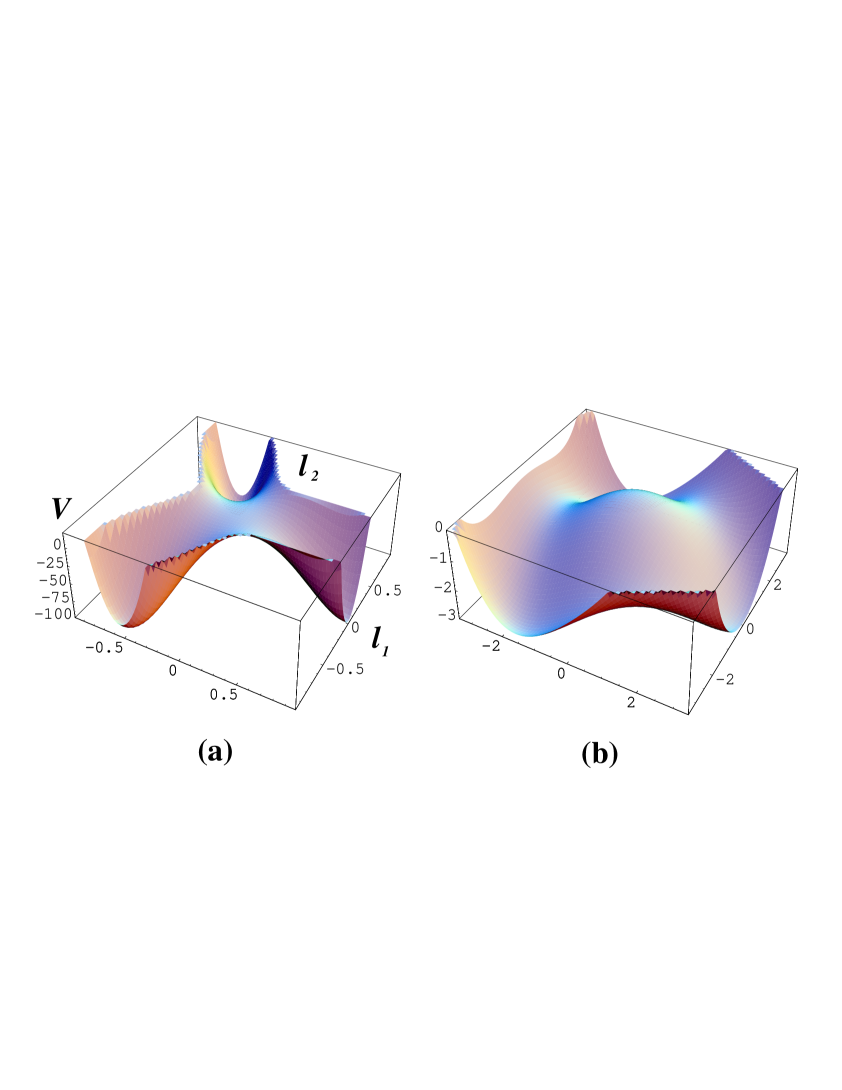
FIG. 2.:

(a) shows the surface plot of the potential $V(l)$ (in units of $T_{c}^{4}$) in Eq.(4) in the complex $l$ plane for $T=400MeV$. Plot range in the $V$ axis is restricted to make the $Z(3)$ barriers and the central bump distinctly visible. It is clearly seen that the barrier between different $Z(3)$ vacua is higher than the central bump. To compare this situation with a standard axionic model case (with same $Z(3)$ symmetry), we show in (b) the plot of the potential (divided by $10^{4}$) in Eq.(4) with the coefficient $b_{2}$ multiplied by 100. This makes the barrier between different $Z(3)$ vacua lower than the central bump.

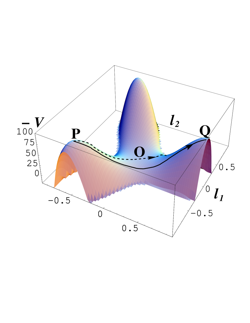
FIG. 3.:

Plot of the inverted potential, i.e. $-V(l_{1},l_{2})$. Again, to show the potential shape clearly, plot range is restricted for negative values. The domain wall solution will correspond to the particle trajectory starting at the top of one of the hills, say, at $P$, and ending at the other hill, say at $Q$. The patricle starting at $P$, and rolling down to $l=0$ (point O in the figure) cannot turn back to end up at $Q$. It will rather go to the other side and roll away downwards, as shown by the dashed curve in the figure. To end up at $Q$, the trajectory must loop back before reaching $l=0$, as shown by the solid curve in Fig.3.

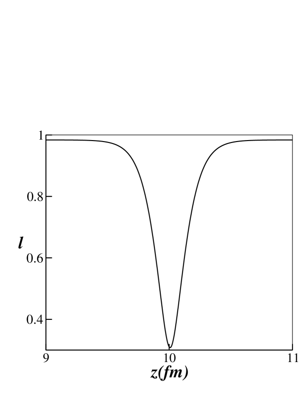
FIG. 4.:

The profile for the domain wall solution (centered near $z=10$ fm) for $T=400MeV$. Note that $l$ remains non-zero inside the wall, with the lowest value of $l$ being about 0.3. Wall thickness (where $l\simeq$ 0.9) is seen to be about 0.5 fm.

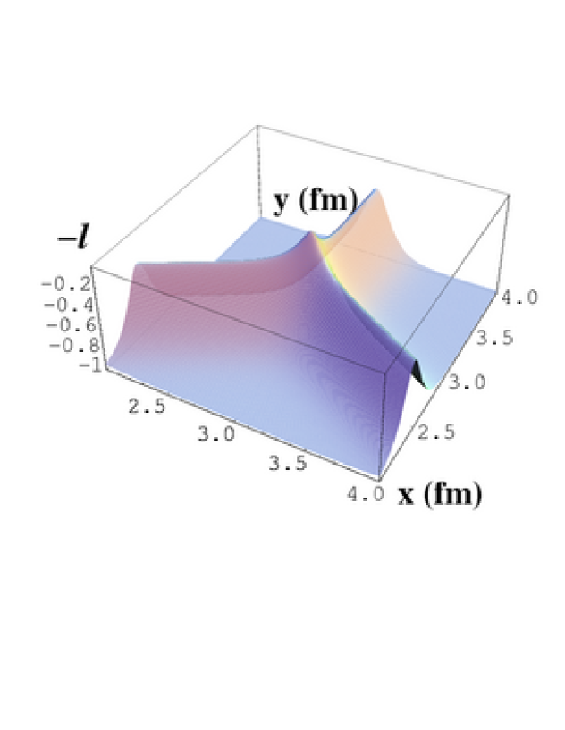
FIG. 5.:

Surface plot of $-l$ for a small portion of the two dimensional lattice showing clearly the profile of the string, connected to three interfaces.

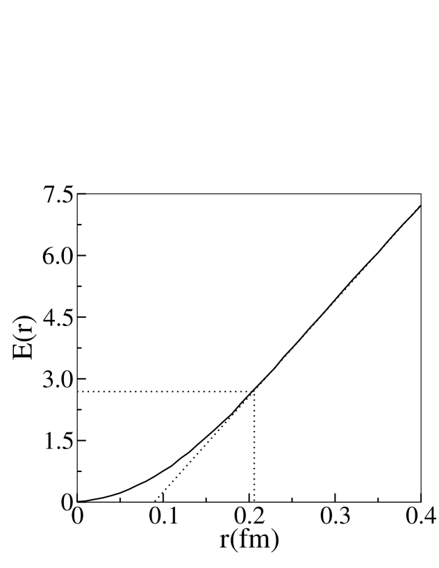
FIG. 6.:

Plot of $E(r)$ in GeV/fm vs. $r$. Simulation results are shown by the solid curve. Dashed line shows the fitting of the large $r$ part of the plot with a straight line. Its slope is found to be about 23 GeV/fm² giving the value of $\sigma\simeq 7.7$ GeV/fm². The core energy $E_{0}(r_{0})=E(r_{0})$ (Eq.(8)) is identified to be equal to $E(r)$ at the value of $r$ where $E(r)$ starts deviating (for decreasing $r$) from the linear fit shown by the dashed line. This is shown in the figure, with $E_{0}$ found to be about 2.7 GeV/fm.

REFERENCES

- [1] L.D. McLerran and B. Svetitsky, Phys. Rev. D24, 450 (1981); B. Svetitsky, Phys. Rept. 132,1 (1986).
- [2] T. Bhattacharya, A. Gocksch, C.K. Altes, and R.D. Pisarski, Nucl. Phys. B383, 497 (1992); S.T. West and J.F. Wheater, Nucl. Phys. Proc. Suppl. 47, 535 (1996); J. Boorstein and D. Kutasov, Phys. Rev. D51, 7111 (1995).
- [3] A.V. Smilga, Annals Phys. 234, 1 (1994).
- [4] V.M. Belyaev, Ian I. Kogan, G.W. Semenoff, and Nathan Weiss, Phys. Lett. B277, 331 (1992);
- [5] C.P. Korthals Altes, hep-th/9402028
- [6] R.D. Pisarski, Phys. Rev. D62, 111501 (2000); ibid, hep-ph/0101168.
- [7] A. Dumitru and R.D. Pisarksi, Phys. Lett. B 504, 282 (2001); Phys. Rev. D 66, 096003-1 (2002); Nucl. Phys. A698, 444 (2002).
- [8] D. Diakonov and M. Oswald, hep-ph/0403108
- [9] S. Chang, C. Hagmann, and P. Sikivie, Phys. Rev. D59, 023505 (1999); M.C. Huang and P. Sikivie, Phys. Rev. D32, 1560 (1985).
- [10] A. Kovner, Phys. Lett. B 509, 106 (2001).
- [11] G. Boyd, J. Engels, F. Karsch, E. Laermann, C. Legeland, M. Lutgemeier, and B. Petersson, Nucl. Phys. B469, 419 (1996); M. Okamoto et al. Phy. Rev. D60, 094510 (1999).
- [12] O. Scavenious, A. Dumitru, and J. T. Lenaghan, Phys. Rev. C66, 034903 (2002)
- [13] S. Coleman, Aspects of symmetry, (Cambridge University Press, 1985).
- [14] A.M. Srivastava, Phys. Rev. D 47, 1324 (1993).