Abstract

In this paper an analytical solution for the high energy scattering amplitude is suggested. This solution has several unexpected features:(i) the asymptotic amplitude is a function of dipole sizes and, therefore, this amplitude shows the gray disc structure at high energy, instead of black disc behaviour which was expected; (ii) the amplitude approaches the asymptotic limit in the same way as the solution to the Balitsky-Kovchegov equation does ($\propto\,\exp(-CY^{2})$ ), but the coefficient $C$ in eight times smaller than for the Balitsky-Kovchegov equation; (iii) the process of merging of two dipoles into one, only influences the high energy asymptotic behaviour by changing the initial condition from $Z(Y;[u_{i}=1])=1$ to $Z(Y;[u_{i}=1-\gamma_{0,i}])=1$. The value of $\gamma_{0}$ is determined by the process of merging of two dipoles into one. With this new initial condition the Balitsky-JIMWLK approach describes the high energy asymptotic behaviour of the scattering amplitude without any modifications recently suggested.

1 Introduction

Our approach to high energy interactions in QCD is based [1, 2] on the BFKL Pomeron [3] and on the reggeon-like diagram technique which takes into account the interactions of BFKL Pomerons [4, 5, 6]. It is well known [7, 8, 9] that the Pomeron diagrams technique can be re-written as a Markov processes [10] for the probability of finding a given number of Pomerons at fixed rapidity $Y$.

However, the colour dipole model provides an alternative approach [11], in which we can replace the non-physical probability to find several Pomerons, by the probability to find a given number of dipoles. It has been shown that everything we had know about high energy interactions can be re-written in the leading $N_{c}$ approximation ($N_{c}$ is the number of colours),in probabilistic approach[11, 12, 13] using dipoles and their interactions. In this approach assuming that we neglect the correlations inside the target, we have a non-linear evolution equation (Balitsky-Kovchegov equation [14, 15], see Ref. [12, 16] for alternative attempts).

The alternative approaches based on the idea of strong gluonic fields [17], or on the Wilson loops approach [14], lead to a different type of theory which is, at first sight, not related to Pomeron interactions. For example the JIMWLK equation [18] appears to be quite different to the Balitsky-Kovchegov equation. However, it has been shown that the Balitsky- JIMWLK approach, is the same as the method based on the dipole model in the leading $N_{c}$ approximation (see Ref. [19, 20]). The further development of the Balitsky - JIMWLK formalism, as well as a deeper understanding the interrelations of this formalism with the old reggeon - like technique based on the BFKL Pomerons and their interactions, is under investigation [20, 21, 22] and we hope for more progress in this direction. Although, the Balitsky-Kovchegov equation is widely used for phenomenology, it has a very restricted region of applicability [23, 24, 25], since it has been derived assuming that only the process of the decay of one dipole into two dipoles is essential at high energy. As was shown by Iancu and Mueller [23] (see also Refs. [24, 25, 26, 27, 28, 29]), a theory neglecting the merging of two dipoles, is not only incorrect, but that the corrections from the process of annihilation of two dipoles into one dipole should be taken into account, to satisfy the unitarity constraint in the $t$-channel of the processes. This, in spite of the fact that there is a $1/N^{2}_{c}$ suppression in the framework of the dipole approach.

A number of papers has been circulated recently [26, 27, 28, 29, 19] in which the key problem of how to include the annihilation of dipoles without losing the probabilistic interpretation of the approach is discussed.

In this paper we find the asymptotic solution to the high energy amplitude using the approach of Ref. [28]. The paper is organized as follows. In the next introductory section we discuss the dipole approach in $1/N^{2}_{c}$ approximation, and consider the main equations which we wish to solve in this paper. We also discuss the statistical interpretation of these equations which play a major role in our method of searching for the solution. The section 3 is devoted to solving the simplified toy model where the interaction does not depend on the size of interacting dipoles. We find here that the large parameters of the problem allow us to use the semi-classical approach for analyzing the solution. In section 4 we find the asymptotic behaviour of the high energy amplitude in the dipole approach including Pomeron loops. We discuss how the amplitude high energy approaches this solution. In the short last section we summarize our results.

2 Generating functional and statistical approach

2.1 Dipole model in $1/N^{2}_{c}$ approximation

The first question that we need to consider is, can we use the dipole approach for calculating $1/N^{2}_{c}$ correction. At first sight the answer is negative . Indeed, Mueller and Chen showed in Ref. [30] that the term of order $\bar{\alpha}_{S}/N^{2}_{c}$ cannot be rewritten as dipole interaction (see Ref. [20], in which this result is demonstrated in the framework of the JIMWLK approach). We consider two dipole rescattering given by Fig. 1. In the leading order in $N_{c}$, the gluon can be emitted by a quark (or antiquark) of one dipole, and should be absorbed by an antiquark (quark) of the same dipole, as is shown in Fig. 1-a. In the next to the leading order in $N_{c}$ the interaction of two dipoles has the form [30, 20]:

$$\frac{\bar{\alpha}_{S}}{N^{2}_{c}}\,\int\,d^{2}z\,K\left(\vec{x}_{1},\vec{y}_{1};\vec{x}_{2},\vec{y}_{2};\vec{z}\right)\,\,\langle T(\vec{x}_{1},\vec{y}_{1}\,x_{2},\vec{y}_{2})\rangle$$ (2.1)

where $T(\vec{x}_{1},\vec{y}_{1}\,x_{2},\vec{y}_{2})$ is the interaction operator for two dipoles, $\bar{\alpha}_{S}=N_{c}\alpha_{S}/\pi$ and

$$K\left(\vec{x}_{1},\vec{y}_{1};\vec{x}_{2},\vec{y}_{2};\vec{z}\right)\,\,=\,\,\left(\frac{(\vec{x}_{1}-\vec{z})_{i}}{(\vec{x}_{1}-\vec{z})^{2}}\,\,-\,\,\frac{(\vec{y}_{1}-\vec{z})_{i}}{(\vec{y}_{1}-\vec{z})^{2}}\right)\,\times\,\left(\frac{(\vec{x}_{2}-\vec{z})_{i}}{(\vec{x}_{2}-\vec{z})^{2}}\,\,-\,\,\frac{(\vec{y}_{2}-\vec{z})_{i}}{(\vec{y}_{2}-\vec{z})^{2}}\right)\,=$$ (2.2)

$$=\,\,\frac{1}{2}\,\left(K(\vec{x}_{2},\vec{y}_{1};\vec{z})\,\,+\,\,K(\vec{x}_{1},\vec{y}_{2};\vec{z})\,\,-\,\,K(\vec{x}_{1},\vec{x}_{2};\vec{z})\,\,-\,\,K(\vec{y}_{1},\vec{y}_{2};\vec{z})\right)$$ (2.3)

where

$$K(\vec{x},\vec{y};\vec{z})\,\,\,=\,\,\frac{(\vec{x}\,-\,\vec{y})^{2}}{(\vec{x}\,-\,\vec{z})^{2}\,\,(\vec{y}\,-\,\vec{z})^{2}}$$ (2.4)

Eq. (2.3) has been discussed in Ref. [31] in the context of the odderon structure in the JIMWLK -approach. The first two terms in Eq. (2.3) describe the emission of a gluon by two dipoles $x_{2}-y_{1}$ and $x_{1}-y_{2}$ (see Fig. 1-b). The configuration in which quark $x_{1}$ (antiquark $y_{1}$) and antiquark $y_{2}$ (quark $x_{2}$) creates a colorless pair is certainly suppressed by factor $1/N^{2}_{c}$. However, after being created dipoles $x_{2}-y_{1}$ and $x_{1}-y_{2}$, will interact as two dipoles in the leading $N_{c}$ approximation (compare Fig. 1 -a and Fig. 1-b). Indeed, the topology of this term is the same as two cylinders . Therefore for the first two terms we can replace $\langle T(\vec{x}_{1},\vec{y}_{1}\,x_{2},\vec{y}_{2})\rangle$ by the product $\langle T(\vec{x}_{1},y_{2})\rangle\,\,\langle\,T(\vec{x}_{2},\vec{y}_{1})\rangle$.

The second two terms in Eq. (2.3) stem from the possibility of two quarks rescattering with a suppression of $1/N^{2}_{c}$. This interaction leads to a quite different topology (see Fig. 1-c), which cannot be treated as two independent parton showers. This new configuration with non-cylindric topology should be treated separately using the so called BKP equation [33], and it is called multi-reggeon Pomeron. Such Pomerons have been studied long ago (see Refs. [34, 35]) and to the best of our knowledge, the intercepts of these $n$-reggeon Pomerons turn out to be smaller than the intercept of $n$ cylindrical configurations (in our case $n=2$).

Therefore, we conclude that we can use the dipole model to even calculate $1/N^{2}_{c}$ corrections. This analysis is supported by direct calculation in Ref. [6], where it is shown that the triple BFKL Pomeron vertex calculated by Bartels in Ref. [4] generates $1/N^{2}_{c}$ corrections which can be rewritten as dipole interactions.

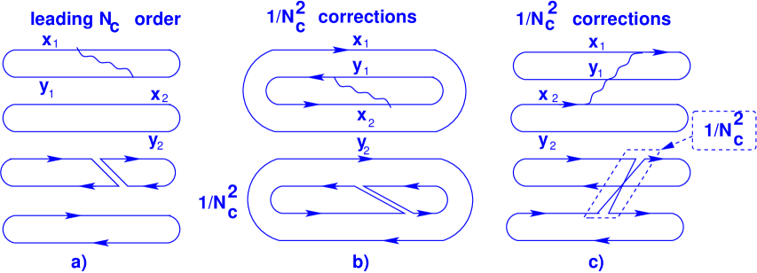
Figure 1: Two dipole rescattering in leading $N_{c}$ order (Fig. 1-a) and $1/N^{2}_{c}$ corrections (Fig. 1-b and Fig. 1-c).Fig. 1-b shows the $1/N^{2}_{c}$ corrections due to re-grouping of the dipoles. This contribution has the same topology as the leading $N_{c}$ order diagram (see Fig. 1-a. Fig. 1-c corresponds to interaction of two quarks from the different dipoles. This contribution has a different topology than Fig. 1-a, and has to be assigned to so called multi-reggeon Pomerons (see for example Ref. [35].

2.2 Main equations

In this section we will discuss the main equations of Ref. [28] paying our attention to their statistical interpretations.

In Ref.[11] the generating functional which characterizes the system of interacting dipoles was introduced, it is is defined as

$$Z\left(Y\,-\,Y_{0};\,[u]\right)\,\,\equiv\,\,$$ (2.5)

$$\equiv\,\,\sum_{n=1}\,\int\,\,P_{n}\left(Y\,-\,Y_{0};\,x_{1},y_{1};\,x_{2},y_{2};\,\dots;x_{i},y_{i};\dots;x_{n},y_{n}\right)\,\,\prod^{n}_{i=1}\,u(x_{i},y_{i})\,d^{2}\,x_{i}\,d^{2}\,y_{i}$$

where $u(x_{i},y_{i})\equiv u_{i}$ is an arbitrary function of $x_{i}$ and $y_{i}$. $P_{n}$ is a probability density to find $n$ dipoles with the size $x_{i}-y_{i}$, and with impact parameter $(x_{i}+y_{i})/2$. Directly from the physical meaning of $P_{n}$ and definition in Eq. (2.5) it follows that the functional (Eq. (2.5)) obeys the condition

$$Z\left(Y\,-\,Y_{0};\,[u=1]\right)\,\,=\,\,1\,.$$ (2.6)

The physical meaning of (Eq. (2.6)) is that the sum over all probabilities is one.

The functional $Z$ has a very direct analogy in the statistical approach: i.e. the characteristic ( generating ) function $\phi(\mathbf{s})$ in Ref. [10]. For $P_{n}$ we have a typical birth-death equation which can be written in the form:

$$\frac{\partial\,P_{n}(\dots,x_{i},y_{i};\dots)}{\partial Y}\,\,\,=$$

$$= \,\,-\sum_{i}\ \Gamma_{1\to 2}\bigotimes\left(P_{n}(\dots,x_{i},y_{i};\dots)\,\,-\,\,\,P_{n-1}(\dots,x_{i},y_{i};\dots)\right)$$

$$\,\,-\sum_{i\neq k}\,\Gamma_{2\to 1}\bigotimes\left(P_{n}(\dots,x_{i},y_{i};\dots)\,-\,P_{n+1}(\dots;x_{i},y_{i};\dots;x_{k},y_{k};\dots)\right)$$

$$\,\,-\sum_{i\neq k}\,\Gamma_{2\to 3}\bigotimes\left(P_{n}(\dots,x_{i},y_{i};\dots;x_{k},y_{k};\dots)\,-\,P_{n-1}(\dots,x_{i},y_{i};\dots;x_{k},y_{k};\dots)\right)$$

In Eq. (2.2) $\Gamma_{1\to 2}$ is the vertex for the process of decay of one dipole with size $x-y$, into two dipoles with sizes $x-z$ and $y-z$. This vertex is well known and it is equal to

$$\Gamma_{1\to 2}\,\,\,=\,\,\bar{\alpha}_{S}\,K(\vec{x},\vec{y};\vec{z})$$ (2.8)

The vertex for the process of transition of two dipoles with sizes $x_{1}-y_{1}$ and $x_{2}-y_{2}$ into three dipoles with sizes $x_{1}-y_{2}$,$z-y_{1}$ and $x_{2}-z$ has been discussed in Ref. [28] and has the form

$$\Gamma_{2\to 3}\,\,=\,\,\frac{\bar{\alpha}_{S}}{2\,N^{2}_{c}}\,\left(K(\vec{x}_{2},\vec{y}_{1};\vec{z})\,+\,K(\vec{x}_{1},\vec{y}_{2};\vec{z})\right)$$ (2.9)

We will discuss the $2\to 1$ vertex we will discuss below.

$\bigotimes$ denotes all necessary integrations (see more detailed form in Ref. [28]). One can see that each line in Eq. (2.2) gives a balance of the death of a particular dipole ( the first term in each line which has a minus sign), and of the birth of two or three dipoles ( the second term in each line which gives a positive contribution . Eq. (2.2) is a typical equation for the Markov’s process ( Markov’s chain) [10].

The last term in Eq. (2.2) has the following form:

$$\Gamma_{2\to 3}\bigotimes\left(P_{n}(\dots,x_{i},y_{i};\dots;x_{k},y_{k};\dots)\,-\,P_{n-1}(\dots,x_{i},y_{i};\dots;x_{k},y_{k};\dots)\right)\,\,=\,\,$$ (2.10)

$$=\,\,\int\,d^{2}x_{i}\,d^{2}x_{k}\,d^{2}y_{i}\,d^{2}y_{k}\,d^{2}z\,\frac{\bar{\alpha}_{S}}{2\,N^{2}_{c}}\,\left(K(\vec{x}_{i},\vec{y}_{k};\vec{z})\,+\,K(\vec{x}_{k},\vec{y}_{i};\vec{z})\right)\,$$

$$\left(P_{n}(\dots,x_{i},y_{i};\dots;x_{k},y_{k};\dots)\,-\,P_{n-1}(\dots,x_{i},y_{i};\dots;x_{k},y_{k};\dots)\right)$$

Multiplying Eq. (2.2) by the product $\prod^{n}_{i=1}\,u_{i}$ and integrating over all $x_{i}$ and $y_{i}$, we obtain the following linear equation for the generating functional:

$$\frac{\partial\,Z\,[\,u\,]}{\partial\,Y}\,\,=\,\,\chi\,[\,u\,]\,\,Z\,[\,u\,]$$ (2.11)

with

$$\chi[u]=$$ (2.12)

$$= -\,\int\,d^{4}\,qd^{4}q_{1}\,d^{4}q_{2}\,\,\left(\Gamma_{1\,\rightarrow\,2}\left(q\to q_{1}+q_{2}\right)\ \left(-u(q)\,+\,u(q_{1})\,u(q_{2})\,\right)\,\frac{\delta}{\delta u(q)}\,-\right.$$ (2.15)

$$\left.-\Gamma_{2\,\rightarrow\,1}\left(q_{1}+q_{2}\to q\right)\,\left(u(q_{1})\,u(q_{2})\,-\,u(q)\right)\,\,\frac{1}{2}\,\frac{\delta^{2}}{\delta u(q_{1})\,\delta u(q_{2})}\right)\,-$$

$$-\int\,\prod^{2}_{i=1}d^{4}q_{i}\,\prod^{3}_{i=1}d^{2}\,z\,\Gamma_{2\to 3}\left((x_{1},y_{1})+(x_{2},y_{2})\to(x_{1},y_{2})+(z,y_{1})+(x_{2},z)\right)\,$$

$$\left(u(x_{1},y_{2})\,-\,1\right)\,\left(u(x_{2},y_{1})\,\,-\,\,\,u(z,y_{1})\,u(x_{2},z)\,\right)\,\frac{1}{2}\,\frac{\delta^{2}}{\delta u(q_{1})\,\delta u(q_{2})}$$

where we denote $d^{4}q_{i}=d^{2}x_{i}\,d^{2}y_{i}$. The functional derivative with respect to $u(q)=u(x,y)$, plays the role of an annihilation operator for a dipole of the size $r=x-y$, at the impact parameter $b=\frac{1}{2}(x+y)$. The multiplication by $u(x,y)$ corresponds to a creation operator for this dipole. Recall that $d^{4}q_{i}$ stands for $d^{2}x_{i}\,d^{2}y_{i}$.

In Eq. (2.12) we subtracted the term that corresponds to the $2\to 3$ transition at $u(x_{1},y_{2})\,=\,1$. Indeed, at $u(x_{1},y_{2})=1$ this transition describes the decay of the colour dipole $(x_{2},y_{1})$ into two dipoles at any size of the dipole $(x_{1},y_{2})$ over which we integrate. Such a process has been taken into account in the first term of Eq. (2.12) which accounts for $1\to 2$ decays of all possible dipoles.

Eq. (2.11) is a typical diffusion equation or Fokker-Planck equation [10], with the diffusion coefficient which depends on $u$. This is the master equation of our approach, and the goal of this paper is to find the asymptotic solution to this equation. In spite of the fact that this is a functional equation we intuitively feel; that this equation could be useful since we can develop a direct method for its solution and, on the other hand, there exist many studies of such an equation in the literature ( see for example Ref. [10]) as well as some physical realizations in statistical physics. The intimate relation between the Fokker-Planck equation, and the high energy asymptotic was first pointed out by Weigert [36] in JIMWLK approach, and has been discussed in Refs. [37, 26, 27].

It should be stressed that in the case of leading $N_{c}$ approximation, the master equation has only the first term with one functional derivative and, therefore, the Fokker-Planck equation degenerates to a Liouville’s equation and describes the deterministic process, rather than stochastic one which the Fokker-Planck equation does. The solution to the Liouville’s equation is completely defined by the initial condition at $Y=0$, and all correlations between dipoles are determined by the correlations at $Y=0$. As has been shown [12, 13, 16] that only by assuming that there are no correlations between dipoles at $Y=0$, we can replace the general Liouville equation by its simplified version, namely, by non-linear Balitsky-Kovchegov equation [14, 15].

2.3 $\Gamma\left(2\to 1\right)$

For further use we need more detailed information on the vertex, for merging of two dipoles in one dipole.

As was shown in Refs. [27, 28, 29] the vertex $\Gamma\left(2\to 1\right)$ can be found from the integral equation which has the form

$$\int\,d^{2}\,x\,d^{2}\,y\,\Gamma_{2\rightarrow 1}\left(x_{1},y_{1}\,+\,x_{2},y_{2}\rightarrow x,y\right)\,\gamma^{BA}\left(x,y;x^{\prime},y^{\prime}\right)\,\,=\,\,$$ (2.16)

$$=\,\,\,\int d^{2}\,x^{\prime}_{1},d^{2}\,y^{\prime}_{1}\,,d^{2}\,x^{\prime}_{2},d^{2}\,y^{\prime}_{2}\,\,\Gamma_{1\rightarrow 2}\left(x^{\prime},y^{\prime}\rightarrow x^{\prime}_{1},y^{\prime}_{1}+x^{\prime}_{2},y^{\prime}_{2}\right)\,\,\gamma^{BA}\left(x_{1},y_{1};x^{\prime}_{1},y^{\prime}_{1}\right)\,\,\gamma^{BA}\left(x_{2},y_{2};x^{\prime}_{2},y^{\prime}_{2}\right)$$

where $\gamma^{BA}$ is a dipole-dipole elastic scattering amplitude in the Born approximation, which is equal [34, 38]

$$\gamma^{BA}\left(x,y;x^{\prime},y^{\prime}\right)\,\,=\,\,\frac{\bar{\alpha}_{S}^{2}}{2\,N^{2}_{c}}\,\frac{1}{16\,\pi^{2}}\,\ln^{2}\left(\frac{(\vec{x}-\vec{x}^{\prime})^{2}\,(\vec{y}-\vec{y}^{\prime})^{2}}{(\vec{x}-\vec{y}^{\prime})^{2}\,(\vec{y}-\vec{x}^{\prime})^{2}}\right)$$ (2.17)

Eq. (2.16) is the basic equation from which the vertex $\Gamma_{2\rightarrow 1}$ can be extracted. To achieve this we need to invert Eq. (2.16), by acting on both sides of it by an operator which is inverse to $\gamma_{BA}$ in operator sense. Fortunately, this operator is known to be a product of two Laplacians [34, 27, 28, 29]:

$$\Gamma_{2\rightarrow 1}\left(x_{1},y_{1}\,+\,x_{2},y_{2}\rightarrow x,y\right)\,\,=\,\,\frac{2N^{2}_{c}}{\bar{\alpha}_{S}^{2}}\,\Delta_{x}\,\Delta_{y}\,\,\,\int d^{2}\,x^{\prime}_{1},d^{2}\,y^{\prime}_{1}\,,d^{2}\,x^{\prime}_{2},d^{2}\,y^{\prime}_{2}\,\times$$ (2.18)

$$\,\Gamma_{1\rightarrow 2}\left(x^{\prime},y^{\prime}\rightarrow x^{\prime}_{1},y^{\prime}_{1}+x^{\prime}_{2},y^{\prime}_{2}\right)\,\,\gamma^{BA}\left(x_{1},y_{1};x^{\prime}_{1},y^{\prime}_{1}\right)\,\,\gamma^{BA}\left(x_{2},y_{2};x^{\prime}_{2},y^{\prime}_{2}\right)$$

The exact evaluation of Eq. (2.18) is done in Ref. [28], but for further presentation in this paper we will need the vertex $\Gamma(2\to 1)$ only in the form of Eq. (2.18).

2.4 Scattering amplitude and its statistical interpretation

As was shown in Refs. [15, 13]) the scattering amplitude is defined as a functional

$$N\left(Y;[\gamma_{i}]\right)\,\, = \,\,-\,\,\int\,\sum^{\infty}_{n=1}\,\frac{(-1)^{n}}{n!}\,\,\,\,\prod^{n}_{i=1}\,d^{2}x_{i}\,d^{2}y_{i}\,\gamma(x_{i},y_{i})\,\frac{\delta}{\delta u_{i}}Z\left(Y,[u_{i}]\right)|_{u_{i}=1}$$

$$= \,\,-\,\,\int\sum^{\infty}_{n=1}(-1)^{n}\,\,\prod^{n}_{i=1}\,d^{2}x_{i}\,d^{2}y_{i}\gamma(x_{i},y_{i})\,\rho_{n}\left(r_{1},b_{1};\dots r_{n},b_{n};Y_{0}\right)$$ (2.19)

where $\gamma$ denotes an arbitrary function which should be specified from the initial condition at $Y=0$. To calculate the amplitude we need to replace each term $\prod^{n}_{i=1}\gamma(x_{i},y_{i})$ by function $\gamma_{n}(x_{1},y_{1};\dots;x_{n},y_{n})$ which characterizes the amplitude at low energies for simultaneous scattering of $n$ dipoles off the target.

From Eq. (2.4) one can see that

$$\rho_{n}\left(x_{1},y_{1};\dots;x_{n},y_{n}\right)\,\,\,=\,\,\frac{1}{n!}\,\prod^{n}_{i=1}\,\frac{\delta}{\delta\,\,u_{i}}\,Z\left(Y;[u_{i}]\right)|_{u_{i}=1}$$ (2.20)

As was shown by Iancu and Mueller [23] $t$-channel unitarity plays an important if not crucial role in low $x$ physics (see also Refs. [24, 25]). In the context of this paper it should be noted that $t$-channel unitarity as a non-linear relation for the amplitude, is able to determine the unknown parameters in the asymptotic solution. $t$ -channel unitarity for dipole-dipole scattering can be written in the form (see Fig. 2)

$$N(x,y;x^{\prime},y^{\prime};Y)\,\,=\,\,$$ (2.21)

$$\sum^{\infty}_{n=1}\,\,\int\,\prod^{n}_{i=1}\,d^{2}x_{i}\,d^{2}y_{i}\,\,\tilde{N}^{p}(x,y;\dots;x_{i},y_{i};\dots x_{n},y_{n};Y-Y^{\prime})\,\tilde{N}^{t}(x^{\prime},y^{\prime};\dots;x_{i},y_{i};\dots x_{n},y_{n};Y^{\prime})\$$

where $\tilde{N}^{p}$ and $\tilde{N}^{t}$ denote the amplitude of the projectile and target, respectively. Actually, they are not exactly the amplitude. Indeed, accordingly Eq. (2.21) their dimension should be $1/x^{2}$ while the amplitude $N$ is dimensionless. On the other hand, we know that the unitarity constraint has a form $Im\,\,N\,\,=\,\,\sum_{n}\,N(2\to n)\,n^{*}(2\to n)$ illustrated in Fig. 2. However, the amplitude in this relation should be taken in the momentum representation, while we here consider the amplitude in the coordinate representation. The difference is clear from Eq. (2.4) where we have that the amplitude of interaction at low energy $\gamma(x_{i},y_{i})$ has been taken into account in the definition of $N$. On the other hand in the unitarity constraints, these amplitudes should only be included once for both amplitudes (see Fig. 3). The general way to do this is to re-write the unitarity constraints through the function $\rho_{n}$ using Eq. (2.20).

It leads us to the following form of the $t$-channel unitarity constraint:

$$N\left(x,y,;x^{\prime},y^{\prime};Y\right)\,\,\,=$$

$$= \,\,\,\sum^{\infty}_{n=1}\,\,(-1)^{n}\,n!\,\int\,\,\prod^{n}_{i=1}\,\,d^{2}\,x_{i}\,\,d^{2}\,y_{i}\,\,\,\prod^{n}_{i=1}\,\,d^{2}x^{\prime}_{i}\,\,d^{2}\,y^{\prime}_{i}\,\,\,\gamma^{BA}(x_{i},y_{i};x^{\prime}_{i},y^{\prime}_{i})\,\,$$

$$\rho^{p}_{n}\left(x,y;x_{1},y_{1};\dots\,x_{i},y_{i};\dots;\,x_{n}\,y_{n},Y-Y^{\prime}\right)\,\rho^{t}_{n}\left(x^{\prime},y^{\prime};x^{\prime}_{1},y^{\prime}_{1};\dots\,x^{\prime}_{i},y^{\prime}_{i};\,\dots;\,x^{\prime}_{n},y^{\prime}_{n};Y^{\prime}\right)\,\,$$

The factor $n!$ appears in Eq. (2.4) is due to the fact that each dipole with rapidity $Y^{\prime}$ from the target can interact with any dipole from the projectile (see Fig. 3).

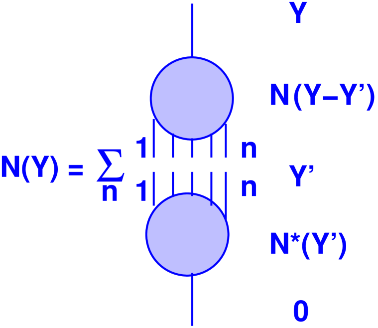
Figure 2: The unitarity constraint in $t$-channel.

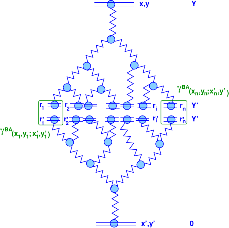
Figure 3: An example of enhanced diagrams that contribute to the unitarity constraint in $t$-channel. Zigzag lines denote the BFKL Pomerons. This particular set of diagrams can be summed by the unitarity in $t$ channel and corresponds to Iancu-Mueller approach [23, 24].

The unitarity constraint itself shows that the high energy amplitude could be described as a Markov process. Indeed, this constraint claims that the amplitude at later time ( $Y+\Delta Y$) is determined entirely by the knowledge of the amplitude at the most recent time ($Y$) since $N(Y+\Delta Y)=N(\Delta Y)\,N(Y)$ from $t$-channel unitarity.

The relation between $Z$ and $N$ is very simple [15], namely

$$N\left(Y,[\gamma_{i}]\right)\,\,\,=\,\,1\,\,\,-\,\,\,Z\left(Y,[1\,-\,\gamma_{i}]\right)$$ (2.23)

Therefore, the amplitude $N$ is closely related to the characteristic function in the statistical approach. However, it is well known that it is better to use the cumulant generating function which is the logarithm of the characteristic function. In our case, we introduce the cumulant generating functional, namely,

$$\Phi\left(Y;[\gamma_{i}]\right)\,\,\equiv\,\,\ln Z\left(Y;[\gamma_{i}]\right)\,\,=\,\,\sum^{\infty}_{n=1}\int\prod^{n}_{i=1}\,d^{2}x_{i}\,d^{2}y_{i}\gamma_{i}\left(x_{i},y_{i}\right)\,p_{n}\left(\dots;x_{i},y_{i};\,\dots\right)$$ (2.24)

where $u_{i}=1-\gamma_{i}$. Eq. (2.24) is the definition for functions $p_{n}$ which are related to cumulants. For example $p_{2}$ is related to $\langle|T(r_{1})T_{[}r_{2})|\rangle-\langle|T(r_{1})\rangle\langle|T(r_{2})\rangle$ rather than to $\langle|T(r_{1})T_{[}r_{2})|\rangle$ as $P_{n}$ does. $T$ is the scattering operator.

The advantage of using $\Phi$ is the following: (i) if there are no correlations between dipoles it is necessary and sufficient to keep only the first term in the series of Eq. (2.24); (ii) to take into account the two dipole correlations we need to keep the two first terms in Eq. (2.24); and (iii) the $n$-term in the series of Eq. (2.24) describes the correlations between $n$-dipoles.

Substituting Eq. (2.24) in Eq. (2.11) we obtain the equation for $\Phi$

$$\frac{\partial\Phi\left(Y;[\gamma_{i}]\right)}{\partial\,Y}\,\,=\,\int d^{4}qd^{4}q_{1}d^{4}q_{2}\,\Gamma(q\to q_{1}+q_{2})\,\left(\gamma(q)\,-\,\gamma(q_{1})\,\gamma(q_{2})\,\right)\,\frac{\delta}{\delta\gamma(q)}\,\Phi\left(Y;[\gamma_{i}]\right)\,\,+$$ (2.25)

$$+\,\,\frac{1}{2}\int d^{4}qd^{4}q_{1}d^{4}q_{2}\,\Gamma(q_{1}+q_{2}\to q)\,\left(\gamma(q)\,-\,\gamma(q_{1})\,\gamma(q_{2})\right)\,\times$$

$$\left(\frac{\delta}{\delta\gamma(q_{1})}\,\Phi\left(Y;[\gamma_{i}]\right)\,\frac{\delta}{\delta\gamma(q_{2})}\,\Phi\left(Y;[\gamma_{i}]\right)\,+\,\frac{\delta^{2}}{\delta\gamma(q_{1})\,\delta\gamma(q_{2})}\,\Phi\left(Y;[\gamma_{i}]\right)\right)\,\,-$$

$$\,\,+\,\,\frac{1}{2}\int\prod_{i=1}^{2}d^{4}q_{i}d^{2}z\,\Gamma(q_{1}+q_{2}\to(x_{1},y_{2})+(x_{2},z)+(z,y_{1}))\,\gamma(x_{1},y_{2})\,\left(\gamma(x_{2},y_{1})\,\,-\,\,\gamma(x_{2},z)\,\gamma(z,y_{1})\,\,\right)\,\times$$

$$\left(\frac{\delta}{\delta\gamma(q_{1})}\,\Phi\left(Y;[\gamma_{i}]\right)\,\frac{\delta}{\delta\gamma(q_{2})}\,\Phi\left(Y;[\gamma_{i}]\right)\,+\,\frac{\delta^{2}}{\delta\gamma(q_{1})\delta\gamma(q_{2})}\,\Phi\left(Y;[\gamma_{i}]\right)\right)$$

where $u(q)\,\equiv\,1\,-\,\gamma(q)$.

3 Asymptotic solution in the toy-model

3.1 General description

We start to solve the master equation (see Eq. (2.11) and Eq. (2.25)) by considering a simple toy model in which we assume that interaction does not depend on the size of dipoles (see Refs. [11, 12, 24] for details). For this model the master functional equation ( see Eq. (2.11) ) degenerates into an ordinary equation in partial derivatives, namely

$$\frac{\partial\,Z}{\partial Y}\,\,=$$ (3.26)

$$=\,\,-\Gamma(1\rightarrow 2)\,\,u(1-u)\,\frac{\partial\,Z}{\partial u}\,\,+\,\,\Gamma(2\rightarrow 1)\,\,u^{(}1-u)\,\,\frac{\partial^{2}\,Z}{(\partial u)^{2}}\,\,+\,\,\Gamma(2\rightarrow 3)u\,(1-u)^{2}\frac{\partial^{2}\,Z}{(\partial u)^{2}}$$

To obtain the scattering amplitude we need to replace $\gamma$ in Eq. (2.23), by the amplitude of interaction of the dipole with the target. For $N$ Eq. (3.26) can be rewritten in the form:

$$\frac{\partial\,N}{\partial Y}\,\,=$$ (3.27)

$$=\,\,\,\Gamma(1\rightarrow 2)\,\,\gamma(1-\gamma)\frac{\partial\,N}{\partial\gamma}\,\,+\,\,\Gamma(2\rightarrow 1)\,\,\gamma(1-\gamma)\,\,\frac{\partial^{2}\,N}{(\partial\gamma)^{2}}\,\,+\,\,\Gamma(2\rightarrow 3)\gamma^{2}\,(1-\gamma)\frac{\partial^{2}\,N}{(\partial\gamma)^{2}}$$

if $\gamma$ is small we can reduce Eq. (3.27) to the simple equation

$$\frac{\partial\,N}{\partial Y}\,\,=\,\,\Gamma(1\rightarrow 2)\,\,\gamma\,\frac{\partial\,N}{\partial\gamma}$$ (3.28)

which has the solution

$$N\,\,=\,\,\gamma e^{\Gamma(1\rightarrow 2)Y}$$ (3.29)

which describes the exchange of the Pomeron with the intercept $\Gamma(1\rightarrow 2)$.

All other terms in Eq. (3.27) have a very simple physical meaning, describing Pomeron interactions (see Fig. 4).

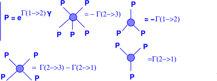
Figure 4: Pomeron interactions described by Eq. (3.27).

The probabilistic approach that we develop in this paper has an advantage that we can apply the well developed formalism of the statistical physics [10] to the partonic system (see Refs. [9, 37, 26, 27] where statistical approach has been applied to our problems). It is reasonable to do this if we are dealing with a system with a large number of dipoles at high energy. We will try to illustrate this point below, but first let us describe the strategy that we will follow in our search for a solution.

3.2 The strategy of our search for the solution

Generally speaking the solution to Eq. (3.26) or to Eq. (3.27) can be written in the form

$$Z(Y;u)\,\,=\,\,Z(\infty;u)\,+\,\Delta Z(Y,u)$$ (3.30)

where asymptotic solutions $Z(\infty;u)$ or $N(\infty;u)$, are solutions of Eq. (3.26) or Eq. (3.27) with the l.h.s. equal to zero, namely, it means that asymptotic form of $Z$ can be determined from the equation

$$\,\,-\,\,\Gamma(1\rightarrow 2)\,\,u\,(1-u)\frac{\partial\,Z(\infty;u)}{\partial\,u}\,\,+$$ (3.31)

$$+\,\,\Gamma(2\rightarrow 1)\,\,u\,(1-u)\,\,\frac{\partial^{2}\,Z(\infty;u)}{\partial\,u^{2}}\,\,+\,\,\Gamma(2\rightarrow 3)u\,(1-u)^{2}\frac{\partial^{2}\,Z(\infty;u)}{\partial\,u^{2}}=0$$

If we prove that the solution $\Delta Z(Y,u)$ which satisfies the full Eq. (3.26) decreases at high energy ( at $Y\to\infty$) the asymptotic solution will give us the behaviour of the scattering ampllitude at high energy.

Eq. (3.26) and Eq. (3.27) are diffusion equations, in which the diffusion coefficient is a function of $u$ or $\gamma$. Let us solve the simplified problem replacing Eq. (3.26) by the equation with constant coefficient, namely,

$$\frac{\partial\,Z}{\partial{\cal Y}}\,\,=\,\,\,-\,\frac{\partial\,Z}{\partial u}\,\,+\,\,\frac{1}{\kappa}\frac{\partial^{2}\,Z}{\partial u^{2}}$$ (3.32)

where ${\cal Y}=\Gamma(1\to 2)\,Y$ and $\kappa$ is defined in Eq. (3.36).

Then

$$Z(\infty,u)\,\,\,=\,\,\,e^{\kappa\,(u-1)}$$ (3.33)

in which we fixed all constants, assuming that all other solutions give small contributions at large values of $Y$ and $Z(\infty;u=1)=1$.

The general solution for Eq. (3.32) is known, namely, it is equal to

$$\Delta Z(Y;u)\,\,=\,\,\frac{1}{2}\,\sqrt{\pi\,\kappa}\,\exp\left(\,-\,\kappa\,\frac{(u\,-\,{\cal Y})^{2}}{4\,{\cal Y}}\right)$$ (3.34)

Eq. (3.34) is the Green function of Eq. (3.32), and using it one can construct the solution for any initial condition. This solution vanishes at large ${\cal Y}$. This fact shows that Eq. (3.33) is the asymptotic solution at high energy.

Therefore, the strategy of searching for the solution to our problem consists of two steps:

1. Finding the asymptotic solution as a solution to Eq. (2.11) with zero l.h.s.;

2. Searching for a solution to the full equation, but assuming that this solution will be small at high energies ($Y\,\to\,\infty$).

We also have to show that the solution, which we find, satisfies the initial condition which we take $Z(Y=0,u)=u$.

In the following presentation we consider separately two cases $\Gamma(2\to 3)=$ and $\Gamma(2\to 1)=0$ which lead us to further understanding of the asymptotic behaviour of the scattering amplitude.

3.3 Solution for $\Gamma(2\to 3)=0$

3.3.1 Asymptotic solution

Considering a simple case with $\Gamma(2\to 3)=0$ we obtain a solution for $Z(\infty;u)$ from Eq. (3.31)

$$Z(u;Y\,\to\,\infty)\,\,=\,\,1-B\,+\,Be^{\kappa(u-1)}$$ (3.35)

where

$$\kappa\,=\,\,\frac{\Gamma(1\,\to\,2)}{\Gamma(2\,\to\,1)}\,\,=\,\,\frac{2\,N^{2}_{c}}{\bar{\alpha}_{S}^{2}}\,\,\gg\,\,1\,\,;\,\,\,\,\,\,\,\,\,\tilde{\kappa}\,\,=\,\,\frac{\Gamma(1\,\to\,2)}{\Gamma(2\,\to\,3)}\,\,=\,\,2\,N^{2}_{c}\,\,\gg\,\,1$$ (3.36)

It should be stressed that in the toy model we keep the same order of magnitude for the vertices as in the full QCD approach. This explains all numerical factors in Eq. (3.36). To avoid any confusion we would like to draw the reader attention to the fact that we will use $\kappa$ and $\tilde{\kappa}$ in further discussions to denote the combination of $\alpha_{S}$ and $N_{c}$ but not the ratios of the vertices which are functions of coordinates in the general case. These combinations give the order of magnitude for the ratios of vertices as far as the $\bar{\alpha}_{S}$ and $N_{c}$ factors are concerned.

Eq. (3.35) satisfies the initial condition that $Z(u=1;Y)\,=\,1$, but the coefficient $B$ remains undetermined, since we cannot use the initial condition at $Y=Y_{0}$. We will show below that the unitarity constraint in $t$-channel will determine $B=1$. Expanding Eq. (3.35) we obtain:

$$\lim_{Y\to\infty}P_{0}(Y)\,\,=\,\,e^{-\kappa};\,\,\,\,\,\,\,\,\,\,\,\lim_{Y\to\infty}P_{n}(Y)\,\,=\,\,\frac{\kappa^{n}}{n!}\,\,e^{-\kappa};$$ (3.37)

We obtained the Poisson distribution with the average number of dipoles $\langle n\rangle=\kappa\,\,\gg\,\,1$. Hence we will attempt to discuss the evolution of our cascade using statistical methods .

To find the value of $B$ in Eq. (3.37) we can use the unitarity constraint in $t$-channel, which can be obtained from Eq. (2.4), and which for the simple model reads as [9, 23, 24, 13]

$$N(Y)\,\,=\,\,\sum^{\infty}_{n=1}\,(-1)^{n}\,n!\,\frac{1}{\kappa^{n}}\rho^{p}_{n}(Y-y)\rho^{t}_{n}(y)$$ (3.38)

where $\rho$ both for the projectile and the target is defined by Eq. (2.21). Eq. (3.38) corresponds to a simplification that in the toy model $\gamma^{BA}\,=\frac{1}{\kappa}\,\delta(x_{i}-x^{\prime}_{i})\,\delta(y_{i}-y^{\prime}_{i})$.

Rewriting Eq. (3.38) for $Y-y\,\gg\,1$ and $y\,\gg\,1$ and taking into account Eq. (2.23) we have

$$N(\infty)\,=\,\sum^{\infty}_{n=1}\,(\frac{-1}{\kappa})^{n}\,n!\,\rho^{p}_{n}(\infty)\,\,\rho^{t}_{n}(\infty)$$ (3.39)

Therefore, we see that $B=1$ since for large $\kappa$ Eq. (3.39) reads as

$$B\,=\,B^{2}$$

Substituting $\rho^{p}_{n}(\infty)=\kappa^{n}_{p}/n!$ and $\rho^{t}_{n}(\infty)=\kappa^{n}_{t}/n!$ we obtain

$$N(\infty)\,\,=\,\,1\,\,-\,\,e^{-\frac{\kappa^{p}\,\kappa^{t}}{\kappa}}\,\,=\,\,1\,\,-\,\,e^{-\kappa}$$ (3.40)

where $\kappa^{p}$ and $\kappa^{t}$ are related to the projectile and target, and they are equal $\kappa^{p}=\kappa^{t}\,=\,\kappa$ in our case. The unitarity constraint determines the value of $u$ in the solution of Eq. (3.35) which is relevant to the asymptotic behaviour of the amplitude. We can translate the result of using unitarity given by Eq. (3.40), as the $u=0$ contribution to the asymptotic behaviour of the amplitude, if we calculate it from Eq. (3.35).

3.3.2 Search for energy dependent solution

Eq. (3.35) leads us to use the Poisson representation [9]:

$$P(Y)\,=\,\int\,\,d\,\alpha\,F(\alpha,Y)\left(\frac{\alpha^{n}}{n!}\,e^{-\alpha}\right)\,\equiv\,\langle P_{n}(\alpha)\rangle$$ (3.41)

where $<\dots>$ stands for averaging with weight $F(\alpha,Y)$.

The generating function $Z(Y;u)$ can be written as

$$Z(Y;u)\,\,=\,\,\int\,\,d\alpha\,\,F(\alpha,Y)\,e^{(u\,-\,1)\,\alpha}$$ (3.42)

Our master equation (see Eq. (3.26)) can be rewritten as

$$\frac{\partial\,F(\alpha,Y)}{\partial\,Y}\,\,=\,\,\,-\frac{\partial}{\partial\,\alpha}\,\left(A(\alpha)\,F(\alpha,Y)\right)\,\,+\,\,\frac{1}{2}\,\frac{\partial^{2}}{\partial\,\alpha^{2}}\,\left(B(\alpha)\,F(\alpha,Y)\right)$$ (3.43)

where

$$A(\alpha)\,\, = \,\,\Gamma(1\,\to\,2)\,\alpha\,-\,\Gamma(2\,\to\,1)\,\,\alpha^{2}\,;$$ (3.44)

$$B(\alpha)\,\, = \,\,2\,A(\alpha);$$ (3.45)

Eq. (3.43) is an equation of Fokker-Planck type ( see Refs. [9, 37, 26, 27] with positive diffusion coefficient $B(\alpha)$ at least for $\alpha<\kappa$. The initial condition of Eq. (2.6) gives the normalization of $F(\alpha,Y)$, namely,

$$\int\,d\,\alpha\,F(\alpha,Y)\,\,=\,\,1$$ (3.46)

For positive $B(\alpha)$ the distribution function $F(\alpha,Y)$ is positive with the normalization of Eq. (3.46), and therefore can be considered as a probability distribution [10]. Hence, the energy dependence of the scattering amplitude can be given by averaging of Eq. (3.40), namely,

$$N(Y)\,=\,$$ (3.47)

$$=\langle\langle N^{(\alpha,\bar{\alpha}}\rangle\rangle\,\equiv\,\int\,\,d\alpha\,F(\alpha,Y-y)\,\,\int\,\,d\bar{\alpha}\,F(\bar{\alpha},y)\,\,\left(1\,\,-\,\,e^{-\alpha\,\bar{\alpha}}\right)$$

Eq. (3.43) is equivalent to the differential stochastic equation [10]

$$d\,\alpha\,=\,A(\alpha)\,+\,\sqrt{B(\alpha)}\,d\,W(Y)$$ (3.48)

where $d\,W(Y)$ is a stochastic differential for the Wiener process. Using Eq. (3.48), together with the large number of dipoles involved in the process is the reason we hope to solve the whole problem using the statistical approaches (see Refs. [9, 26, 27]). However, it is too early to judge how successful this approach will be.

As one can see from Eq. (3.48) $\alpha$ grows until it reaches the zero of $B(\alpha)$ and it becomes frozen at this value at large $Y$. Therefore, we can solve Eq. (3.43) at large energy assuming that $\kappa-\alpha\,\ll\,\kappa$. In this limit $A(\alpha)$ can be replaced by $A(\alpha)\,=\,\kappa-\alpha=\xi$ and Eq. (3.43) reduces to the form

$$\frac{\partial F(\alpha)}{\partial\,{\cal Y}}\,\,=\,\,F(\alpha)\,\,(\xi\,+\,2)\frac{\partial F(\alpha)}{\partial\,\xi}\,\,+\,\,\xi\,\frac{\partial^{2}\,F(\alpha)}{\partial\,\xi^{2}}$$ (3.49)

where ${\cal Y}\,=\,\Gamma(1\,\to\,2)\,Y$ with the solution

$$F(\alpha,{\cal Y})\,\,=\,\,\int\,\frac{d\,\omega}{2\,\pi\,i}\,e^{\omega\,\,{\cal Y}}\,\,{\cal F}(\alpha,\omega)\,;$$ (3.50)

and

$${\cal F}(\alpha,\omega)\,\,=\,\,\phi(\omega)\,{}_{1}F_{1}\left(1+\omega,2,\xi\right)$$ (3.51)

where ${}_{1}F_{1}$ is the confluent hypergeometric function of the first kind. We should choose the function $\phi(\omega)$ from the normalization condition of Eq. (3.46) and, finally,

$${\cal F}(\alpha,\omega)\,\,=\,\,\frac{1}{2}{}_{1}F_{1}\left(1+\omega,2,\xi\right)$$ (3.52)

To find the asymptotic behaviour of this solution at $Y\,\gg\,1$, reconsider Eq. (3.50) which has the form

$$F(\alpha,Y)\,\,=\,\,\int\,\frac{d\,\omega}{2\,\pi\,i}\,e^{\omega\,\,\Gamma(1\to 2)\,Y}\,\,{}_{1}F_{1}\left(1+\omega,2,\xi\right)$$ (3.53)

We can use the integral representation for ${}_{1}F_{1}$ (see 9.211(1) in Ref. [39]) and return to the Poisson representation of Eq. (3.42). Doing so, the solution has the following form

$$Z(u,Y)\,=\,e^{\kappa(u-1)}\,\Psi\left({\cal Y}\,+\,\ln\left(\frac{1+t}{1-t}\right)\right)$$ (3.54)

where $t\equiv\,2(u-1)$ and the arbitrary function $\Psi$ should be determined from the initial condition. One can see that from $Z(u=1;Y)=1$ this function is equal to 1.

This solution corresponds to the asymptotic solution which does not depend on $Y$ (see Eq. (3.35)). We have to consider a different region of $\alpha$ to find out how our system approaches the asymptotic regime given by Eq. (3.35). Assuming that $\alpha\,\ll\,\kappa$ we can model $A$ and $B$ in Eq. (3.43) by $A(\alpha)=\alpha$. In this case Eq. (3.43) has a simple form

$$\frac{\partial\,F(\alpha,Y)}{\partial\,{\cal Y}}\,\,=\,\,\,-\frac{\partial}{\partial\,\alpha}\,\left(\alpha\,F(\alpha,Y)\right)\,\,+\,\,\,\frac{\partial^{2}}{\partial\,\alpha^{2}}\,\left(\alpha\,F(\alpha,Y)\right)$$ (3.55)

Returning to the variable $t=u-1$ (see Eq. (3.42)) we obtain the equation for $Z$

$$\frac{\partial\,Z(t,Y)}{\partial\,{\cal Y}}\,\,=\,\,-2\,Z(t,Y)\,-t(1+t)\,\frac{\partial\,Z(t,Y)}{\partial\,t}$$ (3.56)

which has the solution

$$Z(t,Y)\,\,=\,\,\frac{(1+t)^{2}}{t^{2}}\,\Xi\left({\cal Y}\,+\,\ln\left(\frac{(1+t)}{t}\right)\right)$$ (3.57)

The solution of the master equation (see Eq. (3.26)) can be written as

$$Z(t,Y)\,\,=\,\,e^{\kappa\,t}\,\,+\,\,\frac{(1+t)^{2}}{t^{2}}\,\Xi\left({\cal Y}\,+\,\ln\left(\frac{(1+t)}{t}\right)\right)$$ (3.58)

Function $\Xi$ is arbitrary function and we determine it from the initial condition that $Z(u,Y=0)=u$. Finally, the solution has the form

$$Z(t,Y)\,\,=\,\,e^{\kappa\,t}\,\,\,+\,\,e^{-2\,\Gamma(1\to 2)\,Y}\,\left(\frac{1+t}{1+t-t\,e^{-\Gamma(1\to 2)\,Y}}\,\,-\,\,\exp\{\kappa\,\frac{t\,e^{-\Gamma(1\to 2)\,Y}}{1+t-t\,e^{-\Gamma(1\to 2)\,Y}}\,\}\right)$$ (3.59)

Therefore, the key difference between the case with only emission of dipoles (only $\Gamma(1\to 2)\,\neq\,0$), and the case when we take into account the annihilation of dipoles $\Gamma(1\to 2)\,\neq\,0$ and $\Gamma(2\to 1)\,\neq\,0$, is the fact that there exists an asymptotic solution which depends on $u$ (see Eq. (3.35)). Eq. (3.59) shows that the energy dependent solution in the wide range of $t$ or $u$ satisfy the initial condition $Z(Y=0;u)=u$ and it decreases at $Y\to\infty$. Therefore, Eq. (3.40) gives the asymptotic solution to our problem.

3.4 Solution for $\Gamma(2\to 1)=0$

3.4.1 Asymptotic solution

For the case $\Gamma(2\to 1)=0$ the system shows quite different behaviour, namely,

$$Z(u;Y\,\to\,\infty)\,\,=\,\,1+\frac{B}{1\,-\,\tilde{\kappa}}\,\left((1-u)^{1-\tilde{\kappa}}\,-\,(1-u_{0})^{1-\tilde{\kappa}}\right)$$ (3.60)

where $\tilde{\kappa}$ is given by Eq. (3.36). Formally speaking we cannot satisfy the boundary condition $Z(u=1;Y\,\to\,\infty)$. The reason for this is obvious, since we cannot take $u$ close to 1 and neglect $\Gamma\left(2\to 1\right)$ term in Eq. (3.26). We can do this only for $u>u_{o}\approx 1-\tilde{\kappa}/\kappa\propto\bar{\alpha}_{S}^{2}$.

One can see that Eq. (3.60) gives

$$<n>=dZ(u;Y\,\to\,\infty)/du|_{u=1}=B(1-u_{0})^{-\tilde{\kappa}}B(\tilde{\kappa}/\kappa)^{-\tilde{\kappa}}\,\,\gg\,1$$

Therefore, once again we hope that the statistical approach can work in this system.

Eq. (3.60) is the asymptotic solution in this case. Once more we should use the unitarity constraint to fixed the parameter $B$. Repeating all calculations that led to Eq. (3.40) we obtain

$$N(\infty)\,=\,\,\sum^{\infty}_{n=1}\,\frac{1}{n!}\,\frac{\Gamma^{2}(\tilde{\kappa}+n)}{\Gamma^{2}(\tilde{\kappa})}\,\left(\,-\,\frac{1}{\kappa\,(1-u_{0})^{2}}\right)^{n}\,\,\equiv$$ (3.61)

$$\equiv\,\,{}_{2}F_{0}\left(\tilde{\kappa},\tilde{\kappa};;-\,\frac{1}{\kappa\,(1-u_{0})^{2}}\right)\,\,<$$

$$<\,1-\exp\left(-\frac{1}{\kappa\,(1-u_{0})^{2}}\right)\,\,+\,\,\exp\left(\,-\,\frac{1}{\kappa\,(1-u_{0})^{2}}\right)\,\,Ei\left(-\kappa(1-u_{o})^{2}\right)$$

where $\Gamma(x)$ is the Euler gamma function, ${}_{2}F_{0}$ is the generalized hypergeometric function[39] and $Ei(x)=\int_{-\infty}^{x}\frac{e^{t}}{t}dt$ is exponential integral. Considering $1-u_{0}\approx\,-\tilde{\kappa}/\kappa$ we see that

$$N(\infty)\,\,\,<\,\,1-\exp\left(-\frac{\kappa}{\tilde{\kappa}^{2}}\right)\,\,+\,\exp\left(\frac{\kappa}{\tilde{\kappa}^{2}}\right)\,Ei\left(-\frac{\kappa}{\tilde{\kappa}^{2}}\right)$$ (3.62)

3.4.2 Solution for $\Delta Z(Y;u)$

As has been shown in Eq. (3.60), the asymptotic distribution at large values of Y is not the Poissonian type. If we try to introduce the distribution function $F(\alpha,Y)$, the equation for it has the form

$$\frac{\partial\,F(\alpha,Y)}{\partial\,\tilde{Y}}\,\,=$$ (3.63)

$$\,\,-\frac{\partial}{\partial\,\alpha}\,\left(\tilde{A}(\alpha)\,F(\alpha,Y)\right)\,\,+\,\,\frac{1}{2}\,\frac{\partial^{2}}{\partial\,\alpha^{2}}\,\left(\tilde{B}(\alpha)\,F(\alpha,Y)\right)\,\,-\,\,\frac{\partial^{3}}{\partial\,\alpha^{3}}\left(\tilde{C}(\alpha)\,F(\alpha,Y)\right)$$

where $\tilde{Y}\,=\,\Gamma(1\,\to\,2)\,Y$ and

$$\tilde{A}(\alpha)\,\, = \,\,\alpha\,-\,\,\frac{1}{\kappa}\,\,\alpha^{2}\,;$$ (3.64)

$$\tilde{B}(\alpha)\,\, = \,\,2\,\alpha\,-2\,\,\left(\,\,\frac{1}{\kappa}\,\,-\,\,\frac{1}{\tilde{\kappa}}\,\,\right)\,\alpha^{2}\,;$$ (3.65)

$$\tilde{C}(\alpha)\,\, = \,\,\frac{1}{\tilde{\kappa}}\,\,\alpha^{2}\,;$$ (3.66)

$\tilde{B}(\alpha)$ does not have a zero and, therefore, we expect that the asymptotic behaviour will be related to the large values of $\alpha$. For the master equation (see Eq. (3.26)) it means that $u\,\to\,1$ will be essential. In the simple case $\Gamma(2\to 1)=0$ and $u\,\to\,1(1-u\,\ll\,1$ the master equation degenerates to

$$\frac{\partial Z(u,Y)}{\Gamma(1\to 2)\partial Y}\,=$$ (3.67)

$$\,-\,u(1-u)\,\frac{\partial Z(u,Y)}{\partial\,u}\,\,+\,\,\frac{(1-u)^{2}}{\tilde{\kappa}}\,\frac{\partial^{2}Z(u,Y)}{\partial\,u^{2}}\,\,\equiv\,(1-\frac{1}{\tilde{\kappa}})\frac{\partial Z(\zeta,Y)}{\partial\,\zeta}\,\,+\,\frac{1}{\tilde{\kappa}}\,\frac{\partial^{2}Z(\zeta,Y)}{\partial\,\zeta^{2}}$$

where $\zeta=\ln(1-u)$. The solution of this equation is simple, namely,

$$Z(\zeta,Y)\,\,=\,\,\int^{a+i\infty}_{a-i\infty}\,\,\frac{d\lambda}{2\,\pi\,i}\,{\cal Z}(\lambda)\,e^{\left((1-\frac{1}{\tilde{\kappa}})\,\lambda\,+\,\frac{1}{\tilde{\kappa}}\,\lambda^{2}\right)\Gamma(1\to 2)\,Y\,+\,\lambda\,\zeta}$$ (3.68)

where ${\cal Z}(\lambda)\,=\,1/(\lambda-1)$ using the initial condition that $Z(u,Y=0)=u$.

The solution which satisfies our initial condition is equal to

$$Z(\zeta,Y)\,\,=\,\,erf\left(\frac{\eta}{2\,\sqrt{\Gamma(1\to 2)Y/\tilde{\kappa}}},\right)$$ (3.69)

where $\eta\,=\,(1+\frac{1}{\tilde{\kappa}})\,\Gamma(1\to 2)\,Y\,\,+\,\,\zeta$ and $erf(x)$ is the error function given by $erf(x)=(2/\sqrt{\pi})\,\int^{x}_{0}\,\,\exp(-t^{2})\,dt$.

At $Y=0$ Eq. (3.69) leads to $Z(\zeta,Y=0)=1\,\approx\,u$, since we assume that $u$ is close to unity.

At $Y\to\infty$ we have

$$Z(\eta,Y\,\to\,\infty)\,\,\to\,\,1\,\,-\,\,\sqrt{\frac{4\,\Gamma(1\to 2)\,\,Y}{\pi\,\tilde{\kappa}\,\,\eta}}\,\,\,\exp\left(-\frac{\eta^{2}\,\tilde{\kappa}}{4\,\Gamma(1\to 2)\,\,Y}\right)$$ (3.70)

Therefore, we have obtained a solution and the only problem, that remains, is the behaviour of the asymptotic solution at $u\,\to\,1$. We need to investigate the region of $u\to 1$, but we will do this using a new approximation, in which we use the large parameters of our approach ( see Eq. (3.36)).

3.5 Semi-classical approach for large $\kappa$ and $\tilde{\kappa}$

Considering the solution of Eq. (3.59), we notice that the function $\Phi$ (see Eq. (2.24) and Eq. (2.25)) for this solution is large and it is proportional to $\kappa$. This observation triggers a search for a semi-classical solution assuming that $\Phi^{2}_{\gamma}>>\Phi_{\gamma,\gamma}$ where $\Phi_{\gamma}\equiv\,dPhi/d\gamma$.

For $\Gamma(2\to 3)=0$ in the toy model Eq. (2.25) has the form

$$\frac{\partial\,\Phi(Y,\gamma)}{\partial\,{\cal Y}}\,=\,\,\gamma(1-\gamma)\,\{\frac{\partial\,\Phi(Y,\gamma)}{\partial\,\gamma}\,\,+\,\,\frac{1}{\kappa}\left(\frac{\partial\,\Phi(Y,\gamma)}{\partial\,\gamma}\right)^{2}\}$$ (3.71)

Fist, we see that the asymptotic solution $\Phi(\infty;\gamma)=-\kappa\,\gamma$ is the same as that we obtained in Eq. (3.35) and Eq. (3.59). We try to find the solution to Eq. (3.71) for all values of $Y$ in the form $\Phi({\cal Y};\gamma)\,\,=\,\,\Phi(\infty;\gamma)\,\,+\,\,\Delta\Phi({\cal Y};\gamma)$ considering $\Delta\Phi\,\,\ll\,\,\Phi(\infty;\gamma)$. For such a solution Eq. (3.71) reduces to a linear equation

$$\frac{\partial\,\Delta\Phi(Y,\gamma)}{\partial\,{\cal Y}}\,=\,\,-\,\gamma(1-\gamma)\,\frac{\partial\,\Delta\Phi(Y,\gamma)}{\partial\,\gamma}$$ (3.72)

The solution to this equation has the form

$$\Delta\Phi(Y,\gamma)\,\,=\,\,H\left({\cal Y}\,+\,\,\ln\left(\frac{\gamma-1}{\gamma}\right)\right)$$ (3.73)

where $H$ is an arbitrary function which should be found from the initial conditions $Z(Y=0,[u_{i}])=u$.

Assuming that $\Delta\Phi\,\ll\,\Phi(\infty,\gamma)$ at $Y=0$, we can reconstruct the solution given by Eq. (3.73), namely,

$$Z(\gamma,Y)\,\,=\,\,\exp\left(\Phi(\infty,\gamma)\,+\,\Delta\Phi(Y,\gamma)\right)\,\,=\,\,$$ (3.74)

$$\frac{1-\gamma}{1-\gamma+\gamma\,e^{-\Gamma(1\to 2)Y}}\,\exp\{-\kappa\,\gamma\,\,+\,\,\kappa\,\frac{\gamma e^{-\Gamma(1\to 2)Y}}{1-\gamma+\gamma\,e^{-\Gamma(1\to 2)Y}}\}$$

This solution differs from the solution given by Eq. (3.59), but leads to the same behaviour at large values of $Y$. The difference is obvious since $\Delta\Phi$ is not small at small values of $Y$.

We attempt to find a solution using the same methods as for the case $\Gamma(2\to 1)=0$.

The asymptotic solution for $\Phi$ is $\Phi(\infty;u)\,\,=\,\,-\tilde{\kappa}\,ln(\gamma)$. This can be seen directly from Eq. (3.60), and it also appears as the solution to the following equation

$$0\,\,=\,\,\gamma\,(1-\gamma)\,\{\frac{\partial\,\Phi(\infty;\gamma)}{\partial\,\gamma}\,\,+\,\,\frac{1}{\tilde{\kappa}}\,\gamma\,\left(\frac{\partial\,\Phi(\infty;\gamma)}{\partial\,\gamma}\right)^{2}\}$$ (3.75)

For $\Delta\Phi(Y,u)$ ($\Phi(Y,u)\,\,=\,\,\Phi(\infty;u)\,\,+\,\,\Delta\Phi(Y,u)$) we have

$$\frac{\partial\,\Delta\Phi(Y;\gamma)}{\partial\,{\cal Y}}\,=\,\,\,\gamma\,(1-\gamma)\,\frac{\partial\,\Delta\Phi(Y;\gamma)}{\partial\,\gamma}$$ (3.76)

A general solution to this equation is

$$\Delta\Phi(Y,\gamma)\,\,=\,\,S\left({\cal Y}\,-\,\ln\left(\frac{\gamma}{\gamma-1}\right)\,\right)$$ (3.77)

where $S$ is an arbitrary function which should be determined from the initial conditions $Z(Y=0;u)=u$ which translates into initial conditions for $\Delta\Phi$ as

$$\Delta\Phi(Y=0,u)\,\,=\,\,\tilde{\kappa}\,\ln(\gamma)\,\,+\,\ln(1-\gamma)$$ (3.78)

Finally, we obtain the solution in the form:

$$Z({\cal Y};\gamma)\,\,=\,\,1\,\,+\,\frac{1-\gamma}{1-\gamma+\gamma e^{-{\cal Y}}}\,\,\left(\,1\,\,-\,\,\gamma\,\,-\,\,\gamma\,e^{-{\cal Y}}\right)^{-\tilde{\kappa}}\,\,$$ (3.79)

This is the solution which tends to the asymptotic solution as $Y\to\infty$, at least at small values of $\gamma\,<\,1/\tilde{\kappa}$. Note, we have not achieved the correct normalization $Z(u=1,Y)=1$. However, we believe this is connected to the problem of ill defined limit of $\Gamma(2\to 1)$, for small $\gamma\ll\tilde{\kappa}/\kappa$. To get a better understanding the situation better we consider the general case in the semi-classical approach.

3.6 Semiclassical approach to a general case

It is easy to obtain the asymptotic solution

$$\Phi(\infty,\gamma)\,\,=\,\,-\,\tilde{\kappa}\,\ln\left(1\,\,+\,\,\frac{\kappa}{\tilde{\kappa}}\,\gamma\right)$$ (3.80)

$\Delta\Phi(Y,u)$ ($\Phi(Y,u)\,\,=\,\,\Phi(\infty;u)\,\,+\,\,\Delta\Phi(Y,u)$) has the form

$$\frac{\partial\,\Delta\Phi(Y;\gamma)}{\partial\,{\cal Y}}\,=\,\,\,\gamma\,(1-\gamma)\,\frac{\partial\,\Delta\Phi(Y;\gamma)}{\partial\,\gamma}$$ (3.81)

and the solution to this equation has the same form as Eq. (3.77), but with a different initial condition:

$$\Delta\Phi(Y=0;\gamma)\,\,=\,\,\tilde{\kappa}\,\ln\left(1\,\,+\,\,\frac{\kappa}{\tilde{\kappa}}\,\gamma\right)\,\,+\,\,\ln\left(1\,-\,\gamma\right)$$ (3.82)

Using the arbitrary function $S$ ( see Eq. (3.77) ) and from Eq. (3.82) we, finally, obtain the answer for the generating functional $Z$

$$Z\left(Y,\gamma\right)\,\,=\,\,\frac{(1-\gamma)\,e^{\Gamma(1\to 2)\,\,Y}\,}{\gamma\,+\,(1-\gamma)\,e^{\Gamma(1\to 2)\,\,Y}}\,\,\left(1\,\,+\,\,\frac{\kappa}{\tilde{\kappa}}\,\gamma\right)^{-\tilde{\kappa}}\,\,\left(1\,+\,\frac{\kappa}{\tilde{\kappa}}\,\frac{\gamma}{\gamma\,+\,(1-\gamma)\,e^{\Gamma(1\to 2)\,\,Y}}\right)^{\tilde{\kappa}}$$ (3.83)

This solution satisfies all requiments: (i) $Z\left(Y,u=1\right)\equiv Z\left(Y,\gamma=0\right)\,=\,1$; (ii) $Z\left(Y=0,u\right)=u\equiv 1-\gamma$; and at $Y\to\infty$ $Z\left(Y,u\right)\,\,\to\,\,Z(\infty,u)$.

The asymptotic solution of Eq. (3.80) leads to the following $Z$

$$Z\left(\infty,\gamma\right)\,\,=\,\,\left(\,1\,\,+\,\,\frac{\kappa}{\tilde{\kappa}}\,\right)^{-\tilde{\kappa}}$$ (3.84)

Using Eq. (2.20) we obtain

$$\rho_{n}\,\,=\,\,\frac{(-1)^{n}}{n!}\,\frac{\Gamma(\tilde{\kappa}+n)}{\Gamma(\tilde{\kappa})}\,\,\left(\frac{\kappa}{\tilde{\kappa}}\right)^{n}$$ (3.85)

This $\rho_{n}$ is the same as for the case of $\Gamma(2\to 1)=0$ (see Eq. (3.60)) if $1-u_{0}$ is chosen to be equal to $1-u_{0}\,\,=\,\,\tilde{\kappa}/\kappa$. It should be stressed that Eq. (3.83) and Eq. (3.85) lead to the scattering amplitude given by Eq. (3.61). It shows that we correctly guessed the value of $1-u_{0}$. Only for $1-u\,\leq 1-u_{o}$ do we have to take into account the process of merging of two Pomerons into one Pomeron. In other words, we can neglect the $2\to 1$ process if we put the initial condition for the generation functional $Z(Y,u)$ at $u=u_{0}$, namely $Z(Y,u=1-\tilde{\kappa}/\kappa)=1$. This property resembles and even supports the idea of Ref. [45], that merging processes suppress correlations when these correlations are small.

3.7 Lessons for searching a general solution

We view this toy model as a training ground to help us find a general solution, and as an aid suggesting directions for such a search. We learned several lessons that will be useful:

1. Our approach in searching for the solution consists of the following steps:

   • Finding the asymptotic solution as the solution to the master equation ( see Eq. (2.11), Eq. (2.25), Eq. (3.26) and Eq. (3.28)) with zero l.h.s.;

   • Using the large parameters of our theory given by Eq. (3.36), we can develop the semi-classical approach for searching both for the asymptotic solution and for the correction to this solution, that provide the form of the generating functional approaching its asymptotic value;

   • The corrections to the asymptotic solution decrease at large values of $Y$, and can be found from the Liouville-type linear equation;

   • The important region of $u$ ($\gamma$) are $u\,\to 1$ and $\gamma\,\to\,0$, which should be specified by using the unitarity constraint;

2. The inclusion of $\Gamma(2\to 3)$ is very crucial for the form of solution;

3. The asymptotic form of the solution differs from the solution to the Balitsky-Kovchegov equation: amplitude $N$ does not approach 1 ($N\rightarrow 1$) at $Y\rightarrow\infty$, but rather $N(\infty,\gamma)$ is a function of $\gamma$. In particular, it means that we do not expect geometrical scaling [40] for the solution to the full set of equations. We also do not expect that the scattering amplitude to show a black disk behaviour on reaching the value of unity at high energies. We predict the gray disc behaviour for this scattering amplitude;

4. It is easy to find the solution using the equation for the cumulant generation functional $\Phi$ (see Eq. (2.24) and Eq. (2.25)).

5. The role of the $2\to 1$ process is very interesting: this process suppresses the small values of $\gamma\,\leq\tilde{\kappa}/\kappa$ in a such way that they can be neglected, supporting the idea of Ref. [45];

It should be stressed that we found such a solution to the simplified evolution equation (see Eq. (3.26)), which has the form of $Z(\infty,u)\,+\,\Delta Z(Y,u)$ with $\Delta Z(Y,u)\,\to\,0$ at large $Y$. It is shown that $\Delta Z(Y,u)$ satisfies the initial condition for the generating functional. Therefore, for the toy model we prove that our solution is the solution to the evolution equation if we believe that we have the only one solution. For the solution to the general evolution equation (see Eq. (2.11) ) we will not be able to show that our solution satisfies the initial condition for the generating functional. Therefore, it is possible that could exist a different solution which we overlooked in our approach but which will satisfy the initial condition while ours does not. This is the reason, why the solution to the evolution equation in the toy model, in which we can check that such situation does not occur, is so important for our approach.

It should be stressed that all new feathures of the solution appear only in the next to leading order in $1/N_{c}$. In the leading order the JIMWLK-B approach leads to a solution with behaves as a black disc.

At first sight, the gray disc behaviour of the scattering amplitude looks unrealistic. However, the situation is just opposite, the gray disc behaviour is rather natural in the parton model (see Ref. [50]) and we have spent a decade to understand how it is possible that we have a black disc behaviour for the scattering amplituide in QCD [51]. The black disc behaviour stems from the simple fact that in JIMWLK-B approach the number of ‘wee” dipoles of each size increases as power of energy due to BFKL emission. It means that the dipoles started to interact with each other even if this interaction is small (proportional to $\alpha_{S}$). At very high energy the probability to find any dipole is equal to unity. The Pomeron loops lead to diminishing of the BFKL Pomeron intercept and, therefore, to a suppression of the number of the ‘wee’ partons. Finally, the increase of the number of ‘wee’ dipoles stops before the probability to find a dipole reaches 1. The entire picture seems to be close to so called critical Pomeron scenario (see Ref. [52]): the only theoretical model of Pomeron that has been solved.

Armed with this knowledge we will now to solve the general equations ( see Eq. (2.11) and /or Eq. (2.25) ).

4 Asymptotic solution (general consideration)

4.1 Solution for $\Gamma(2\to 3)$=0

4.1.1 Solution at $Y\,\to\,\infty$

Our strategy in searching for the solution will be based on the lessons we learnt from the toy model. First we try to solve the master equation (see Eq. (2.25) ) assuming that

$$\,\frac{\delta^{2}\Phi}{\delta\gamma(x_{1},y_{1})\delta\gamma(x_{2},y_{2})} \ll \,\frac{\delta\Phi}{\delta\gamma(x_{1},y_{1})}\frac{\delta\Phi}{\delta\gamma(x_{2},y_{2})}$$ (4.86)

$$\Phi\left(\infty;[\gamma_{i}]\right) = -\kappa\,\,\int\,d^{2}x\,d^{2}y\,\,\Delta_{x}\,\Delta_{y}\phi(x,y;\infty)\,\,\,\gamma(x,y)$$ (4.87)

Substituting Eq. (4.87) into Eq. (2.25) and putting the l.h.s. of Eq. (2.25) to zero, we obtain the following equation for asymptotic solution $\phi(x,y;Y=\infty)$:

$$0\,\,=\,\,\int\,d^{2}\,z\,\,K(\vec{x},\vec{y};\vec{z})\,\Delta_{x}\,\Delta_{y}\,\phi(x,y;\infty)\,\,-\,\,\Delta_{x}\,\Delta_{y}\left(\,\,\int\,d^{2}z\,\,K(\vec{x},\vec{y};\vec{z})\,\,\int\,d^{2}x_{1}\,d^{2}\,y_{1}\,\,\right.$$ (4.88)

$$\left.\gamma^{BA}\left(\vec{x},\vec{z};\vec{x}_{1}\,\vec{y}_{1}\right)\Delta_{x_{1}}\,\Delta_{y_{1}}\phi(x_{1},y_{1};\infty)\,\,\int\,d^{2}x_{2}\,d^{2}y_{2}\,\,\gamma^{BA}\left(\vec{x},\vec{z};\vec{x}_{2}\,\vec{y}_{2}\right)\Delta_{x_{2}}\,\Delta_{y_{2}}\phi(x_{1},y_{1};\infty)\right)$$

where $K$ is given by Eq. (2.4) and we used Eq. (2.18) for the vertex $\Gamma(2\to 1)$. Integrating Eq. (4.88) by parts with respect to $x_{1},y_{1}$ and $x_{2},y_{2}$ and using

$$\Delta_{x_{1}}\,\Delta_{y_{1}}\gamma^{BA}\left(\vec{x},\vec{y};\vec{x}_{1}\,\vec{y}_{1}\right)\,\,\,=\,\,\delta\left(\vec{x}-\vec{x}_{1}\right)\delta\left(\vec{y}-\vec{y}_{1}\right)$$ (4.89)

we find that function $\phi(x,y;\infty)$ satisfies the equation

$$0\,\,=\,\,\int\,d^{2}z\,K(\vec{x},\vec{y};\vec{z})\,\left((\phi(x,y;\infty)\,\,-\,\,\phi(x,z;\infty)\,\phi(z,y;\infty)\right)$$ (4.90)

To obtain Eq. (4.90) from Eq. (4.88) we need to assume that

$$\int\,d^{2}\,z\,\,K(\vec{x},\vec{y};\vec{z})\,\Delta_{x}\,\Delta_{y}\,\phi(x,y;\infty)\,\,\approx\,\,\Delta_{x}\,\Delta_{y}\,\int\,d^{2}\,z\,\,K(\vec{x},\vec{y};\vec{z})\,\,\phi(x,y;\infty)$$ (4.91)

Indeed, as we show below $\Delta_{x}\,\Delta_{y}\,\phi(x,y;\infty)$ is very singular and behaves as $\Delta_{x}\,\Delta_{y}\,\phi(x,y;\infty)\propto\,\delta\left(\vec{x}-\vec{x}_{1}\right)\delta\left(\vec{y}-\vec{y}_{1}\right)$. The function $\int\,d^{2}\,z\,\,K(\vec{x},\vec{y};\vec{z})$ is less singular. Therefore, as far as the most singular part of solution is concerned Eq. (4.91) holds.

The detailed discussion of the solution to Eq. (4.88) will appear in a separate paper [47] and here we will only use the fact that $\phi(x,y;\infty)=1$ satisfies this equation.

Therefore, the cumulant generating functional for the asymptotic solution is equal to

$$\Phi\left(Y;[\gamma_{i}]\right)\,\,=\,\,\kappa\,\,\int\,d^{2}x\,d^{2}y\,\,\Delta_{x}\,\Delta_{y}\phi(x,y;Y)\,\,\,\gamma(x,y)$$ (4.92)

Using Eq. (4.92) and unitarity constraint of Eq. (2.4), we can find the asymptotic behaviour for the scattering amplitude. One can see that the answer is

$$N\left(x,y;x^{\prime},y^{\prime};\infty\right)\,\,=\,\,1\,\,-$$ (4.93)

$$-\,\,\exp\left(-\kappa^{2}\,\int\,\,d^{2}\,\bar{x}\,d^{2}\,\bar{y}d^{2}\,x"\,d^{2}\,y"\Delta_{\bar{x}}\,\Delta_{\bar{y}}\,\phi(x,y;\bar{x},\bar{y},\infty)\,\gamma^{BA}(\bar{x},\bar{y};x",y")\Delta_{x"}\,\Delta_{y"}\phi(x^{\prime},y^{\prime};x",y",\infty)\right)$$

Using the explicit form for $\gamma^{BA}$ as well as Eq. (4.89), we can rewrite Eq. (4.93) in the form:

$$N\left(x,y;x^{\prime},y^{\prime};\infty\right)\,\,=\,\,1\,\,-$$ (4.94)

$$\,\,\exp\left(-\kappa^{2}\frac{\bar{\alpha}_{S}^{2}}{2\,N^{2}_{c}}\,\int\,\,d^{2}\,x"\,d^{2}\,y"\,\phi(x,y;x",y";\infty))\,\Delta_{x"}\,\Delta_{y"}\phi(x^{\prime},y^{\prime};x",y";\infty)\right)$$

where $\phi$ is the solution of Eq. (4.90).

4.1.2 Approaching the asymptotic solution

As in the toy model we will search for a solution in the following form:

$$\Phi\left(Y;[\gamma_{i}]\right)\,\,=\,\,\Phi\left(\infty;[\gamma_{i}]\right)+\Delta\Phi\left(Y;[\gamma_{i}]\right)\,\,$$ (4.95)

assuming Eq. (4.86), and neglecting the contribution $\propto\,(\Delta\Phi)^{2}$.

The resulting equation for $\Delta\Phi\left(Y;[\gamma_{i}]\right)$ has the form

$$\frac{\partial\,\,\Delta\Phi\left(Y;[\gamma_{i}]\right)}{\partial\,{\cal Y}}\,\,=\,\,\,\,\int\,d^{2}x,d^{2}yd^{2}\,z\,d^{2}x_{1}\,d^{2}y_{1}\,d^{2}x_{2}\,d^{2}y_{2}\,\,$$ (4.96)

$$\left(u(x,y)-u(x_{1},y_{1})\,u(x_{2},y_{2})\right)\left(\,\,K(\vec{x},\vec{y};\vec{z})\,\delta\left(\vec{x}-\vec{x}_{1}-\vec{x}_{2}\right)\,\delta\left(\vec{y}-\vec{y}_{1}-\vec{y}_{2}\right)\,\,-\,\,2\,\,\Delta_{x}\,\Delta_{y}\,\,K(\vec{x},\vec{y};\vec{z})\,\,\times\right.$$

$$\left.\gamma^{BA}\left(\vec{x},\vec{z};\vec{x}_{1}\,\vec{y}_{1}\right)\,\,\Delta_{x_{1}}\,\Delta_{y_{1}}\phi(x_{1},y_{1};\infty)\,\,\gamma^{BA}\left(\vec{x},\vec{z};\vec{x}_{2}\,\vec{y}_{2}\right)\right)\frac{\partial\,\,\Delta\Phi\left(Y;[\gamma_{i}]\right)}{\partial\,\gamma(x_{2},y_{2})}$$

Eq. (4.96) is a Liouville-type equation which can easily be solved assuming that the functional $\Delta\Phi\left(Y;[\gamma_{i}]\right)\,=\,\Delta\Phi\left([\gamma_{i}({\cal Y};x_{i},y_{i})]\right)$ . Using this assumption we can re-write

$$\frac{\partial\,\,\Delta\Phi\left({\cal Y};[\gamma_{i}]\right)}{\partial\,{\cal Y}}\,\,=\,\,\int\,d^{2}x\,d^{2}\,y\frac{\partial\,\,\Delta\Phi\left({\cal Y};[\gamma_{i}]\right)}{\partial\,\gamma({\cal Y};x,y)}\,\,\frac{\partial\,\gamma\left({\cal Y};x,y\right)}{\partial\,{\cal Y}}$$

and reduce Eq. (4.96) to the following form:

$$\frac{\partial\,\gamma\left({\cal Y};x,y\right)}{\partial\,{\cal Y}}\,\,=$$ (4.97)

$$\,\,\int\,\,d^{2}\,z\,K(\vec{x},\vec{y};\vec{z})\,\left(u({\cal Y};\vec{x},\vec{y})\,-\,u({\cal Y};\vec{x},\vec{z})\,u({\cal Y};\vec{y},\vec{z})\,\right)\,\,-\,2\,\kappa\,\Delta_{x}\,\Delta_{y}\,\int\,\,d^{2}\,z\,d^{2}\,x_{2}\,d^{2}\,y_{2}K(\vec{x},\vec{y};\vec{z})\,\,\times$$

$$\gamma^{BA}(\vec{x},\vec{z};\vec{x}_{2},\vec{y}_{2})\,\phi(x,z;\infty)\left(\,u({\cal Y};x,y))\,-\,\,u({\cal Y};x_{2},y_{2})\,\,u({\cal Y};x,z)\right)$$

where function $u=1-\gamma$ and $\gamma\left({\cal Y};x,y\right)$ are determined by the initial condition at $Y=0$, namely, at $Y=0$ we have only one dipole with coordinate $x,y$ with

$$\Delta\Phi\left({\cal Y}=0;[\gamma_{i}]\right)\,\,=\ln(1-\gamma({\cal Y}=0,x,y))\,+\,\kappa\,\gamma({\cal Y}=0,x,y)\,\Delta_{x}\,\Delta_{y}\,\phi(x,y,\infty)\,\approx$$ (4.98)

$$\,\,\approx\,\,-\,\,\gamma({\cal Y}=0,x,y)\,+\,\kappa\gamma({\cal Y}=0,x,y)\,\Delta_{x}\,\Delta_{y}\,\phi(x,y,\infty)\,\,\equiv\,\,\Pi(x,y)\,\,\gamma({\cal Y}=0,x,y)$$

Using Eq. (4.98) we can re-write Eq. (4.97) in terms of $\Delta\Phi\left({\cal Y}=0;[\gamma_{i}]\right)$. Neglecting terms of order $(\Delta\Phi)^{2}$ we obtain the following equation

$$\frac{\partial\,\Delta\Phi\left({\cal Y};x,y\right)}{\partial\,{\cal Y}}\,\,=$$ (4.99)

$$\,\,\int\,\,d^{2}\,z\,\left(\,\,K(\vec{x},\vec{y};\vec{z})\,-\ \,2\,\kappa\,\Delta_{x}\,\Delta_{y}\,\int\,\,d^{2}\,x_{2}\,d^{2}\,y_{2}K(\vec{x},\vec{y};\vec{z})\,\,\gamma^{BA}(\vec{x},\vec{z};\vec{x}_{2},\vec{y}_{2})\,\phi(y,z;\infty)\,\,\right)\times$$

$$\left(\,2\,\Pi(x,y)\frac{\Delta\Phi({\cal Y};x,z)}{\Pi(x,z)}\,\,-\,\,\Phi({\cal Y};x,y)\,\right)$$

Eq. (4.99) can be solved in log approximation. The first term in this equation is the familiar BFKL linear equation, therefore, we need to evaluate the second term in Eq. (4.99).

First, we assume that at high energies the nonlinear corrections set the new scale : the saturation momentum $Q_{s}(Y)$ [1, 2, 17] and the integration which we have in the equation is really cut off at $|\vec{x}-\vec{z}|$ and /or $|\vec{y}-\vec{z}|$ smaller than $1/Q_{s}$ [46, 48]. Actually, $\phi(y,z;\infty)$ reaches a maximum value $\phi(y,z;\infty)=1$ which is a solution to Eq. (4.90). We can rewrite $K(x,y;z)$ in the form

$$K(x,y;z)\,\,\equiv\,\,\Delta_{z}\,\ln\left(\frac{(\vec{x}-\vec{z})^{2}}{(\vec{y}-\vec{z})^{2}}\right)$$

Integrating by parts with respect to $z$, and differentiating $\gamma^{BA}$ with respect to $x$ only, we find that the second term has the form

$$2\,\kappa\,\Delta_{x}\,\Delta_{y}\,\int\,\,d^{2}\,x_{2}\,d^{2}\,y_{2}K(\vec{x},\vec{y};\vec{z})\,\,\gamma^{BA}(\vec{x},\vec{z};\vec{x}_{2},\vec{y}_{2})\,\phi(y,z;\infty)\,\,2\,\Pi(x,y)\frac{\Delta\Phi({\cal Y};x,z)}{\Pi(x,z)}\,\,=$$

$$\,\,2\,\kappa\Delta_{y}\,\int\,\,d^{2}\,x_{2}\,d^{2}\,y_{2}\ln\left(\frac{(\vec{x}-\vec{z})^{2}}{(\vec{y}-\vec{z})^{2}}\right)\,\Delta_{x}\,\Delta_{z}\gamma^{BA}(\vec{x},\vec{z};\vec{x}_{2},\vec{y}_{2})\,\,\,2\,\,\Pi(x,y)\frac{\Delta\Phi({\cal Y};x_{2},y_{2})}{\Pi(x_{2},y_{2})}\,=$$ (4.100)

$$=\,\,2\,\int\,\,d^{2}z\,\frac{1}{(\vec{y}-\vec{z})^{2}}\,\Delta\Phi({\cal Y};x,z)$$

where we put $\Pi(x,y)=\Pi(x,z)$ to within the logarithmic accuracy.

Collecting both terms and using Eq. (4.89), we obtain the following equation for $\Delta\Phi$

$$\frac{\partial\,\Delta\Phi\left({\cal Y};x,y\right)}{\partial\,{\cal Y}}\,\,=\,\,-\,\int\,\,d^{2}\,z\,\frac{1}{(\vec{y}-\vec{z})^{2}}\left(\,2\,\Delta\Phi\left({\cal Y};x,z\right)\,\,-\,\,\Delta\Phi\left({\cal Y};x,y\right)\,\right)$$ (4.101)

This is the BFKL equation. However, we solve this equation assuming that $\ln[(\vec{x}-\vec{y})^{2}\,Q^{2}_{s})]\,\,\gg\,\,1$. Considering $|\vec{x}-\vec{z}|\,\ll\,|\vec{x}-\vec{y}|$ we reduce Eq. (4.101) to the following equation

$$\frac{\partial\,\Delta\tilde{\Phi}\left({\cal Y};x,y\right)}{\partial\,{\cal Y}}\,\,=\,\,\int^{(\vec{x}-\vec{y})^{2}}_{\rho^{2}}\,\,\,\frac{d^{2}\,(x-z)}{(\vec{x}-\vec{z})^{2}}\,\,\left(\,2\,\Delta\tilde{\Phi}\left({\cal Y}x,y\right)\right)$$ (4.102)

where $\Delta\tilde{\Phi}\left({\cal Y};x,y\right)=\Delta\Phi\left({\cal Y};x,y\right)/(\vec{x}-\vec{y})^{2}$.

Actually, the typical cutoff $\rho$ is of the order of $\rho^{2}=1/Q^{2}_{s}(Y)$ in the saturation region [46, 48]. Eq. (4.102) can be re-written in the differential form

$$\frac{\partial^{2}\,\Delta\tilde{\Phi}\left({\cal Y};x,y\right)}{\partial\,Y\,\,\partial\,\ln((\vec{x}-\vec{y})^{2}\,Q^{2}_{s}(Y))}\,\,=$$ (4.103)

$$=\,\,-\Delta\tilde{\Phi}\left({\cal Y};x,y\right)\,\,-\,\,\ln((\vec{x}-\vec{y})^{2}\,Q^{2}_{s}(Y))\,\,\frac{\partial\,\Delta\tilde{\Phi}\left({\cal Y};x,y\right)}{\partial\,\ln((\vec{x}-\vec{y})^{2}\,Q^{2}_{s}(Y))}$$

To find the solution to Eq. (4.103) we change the variable introducing a new variable [46, 49, 41, 24]

$$z\,\,=\,\,\ln((\vec{x}-\vec{y})^{2}\,Q^{2}_{s}(Y))\,\,=\,\,\bar{\alpha}_{S}\,\frac{\chi(\gamma_{cr})}{1-\gamma_{cr}}\,Y\,+\,\ln((\vec{x}-\vec{y})^{2}\,Q^{2}_{0})$$ (4.104)

where $\gamma_{cr}$ is determined by the following equation [1, 49, 41]

$$\frac{\chi(\gamma_{cr})}{1-\gamma_{cr}}\,\,=\,\,-\,\,\frac{d\,\,\chi(\gamma_{cr})}{d\,\,\gamma_{cr}}$$ (4.105)

In terms of the new variable, Eq. (4.103) has the form

$$\frac{d^{2}\Delta\tilde{\Phi}(z)}{d\,z^{2}}\,\,=\,\,-\frac{1-\gamma_{cr}}{\chi(\gamma_{cr})}\,\left(\Delta\tilde{\Phi}(z)\,\,-\,\,z\,\frac{d\Delta\tilde{\Phi}(z)}{d\,z}\right)$$ (4.106)

and the solution of Eq. (4.106) is

$$\Delta\Phi\,\,=\,\,\Pi(x,y)\,\gamma(x,y)\,\,\exp\left(-\frac{1-\gamma_{cr}}{2\,\,\chi(\gamma_{cr}))}\,\,z^{2}\,\right)$$ (4.107)

To our surprise the asymptotic behaviour of $\Delta\Phi$ turns out to be the same, as the asymptotic behaviour of the Balitsky-Kovchegov equation [46].

Using the unitarity constraint of Eq. (2.4), and repeating all the calculations that led us to Eq. (4.94) we obtain, that the main corrections to the asymptotic behaviour given by Eq. (4.94) have the form:

$$N\left(x,y;x^{\prime},y^{\prime},Y\right)\,\,=\,\,N\left(x,y;x^{\prime},y^{\prime},\infty\right)\,\,\left(\,1\,-\,\,\int\,d^{2}x"\,d^{2}y"\,\Pi(x,y;x",y")\Pi(x^{\prime},y^{\prime};x",y")\,\times\right.$$

$$\left.\left(\exp\left(-\,\bar{\alpha}_{S}\,\frac{1-\gamma_{cr}}{2\,\,\chi(\gamma_{cr}))}\,\,(Y-Y^{\prime})^{2}\right)\,\,+\,\,\exp\left(-\,\bar{\alpha}_{S}\,\frac{1-\gamma_{cr}}{2\,\,\chi(\gamma_{cr}))}\,\,(Y^{\prime})^{2}\right)\right)\right)$$ (4.108)

We assume in Eq. (4.108) that $Y^{\prime}$ and $Y-Y^{\prime}$ are much larger than $\ln(x-y)^{2}\,Q^{2}_{0}$ or $\ln(x^{\prime}-y^{\prime})^{2}\,Q^{2}_{0}$ . For large $Y$ the minimal corrections occur at $Y^{\prime}=\frac{1}{2}Y$ . Therefore

$$R_{\kappa}\,\,=\,\,\frac{N_{\kappa}\left(x,y;x^{\prime},y^{\prime},Y\right)\,\,-\,\,N_{\kappa}\left(x,y;x^{\prime},y^{\prime},\infty\right)}{N_{\kappa}\left(x,y;x^{\prime},y^{\prime},\infty\right)}\,\,\propto\,\,\exp\left(\,-\,\bar{\alpha}_{S}\,\frac{1-\gamma_{cr}}{8\,\,\chi(\gamma_{cr}))}\,\,(Y)^{2}\,\right)$$ (4.109)

where we denote by $\kappa$ the fact that we consider the example with $\Gamma(2\to 3)=0$.

It is interesting to compare this result with the solutions that have been found :

• For the Balitsky - Kovchegov equation the ratio of Eq. (4.109) is of the order of

  $$R\,\,=\,\,\propto\,\,\exp\left(\,-\,\bar{\alpha}_{S}\,\frac{1-\gamma_{cr}}{2\,\,\chi(\gamma_{cr}))}\,\,(Y)^{2}\,\right)\,\,;$$ (4.110)

• For Iancu-Mueller [23] approach which can be justified only in the limited range of energies we have

  $$R\,\,=\,\,\propto\,\,\exp\left(\,-\,\bar{\alpha}_{S}\,\frac{1-\gamma_{cr}}{4\,\,\chi(\gamma_{cr}))}\,\,(Y)^{2}\,\right)\,\,;$$ (4.111)

Comparing Eq. (4.110) and Eq. (4.111) with Eq. (4.109) we see that the process of merging of two dipoles into one dipole crucially change the approach to the asymptotic behaviour .

4.1.3 Main results

The main results of our approach are given by Eq. (4.108) and Eq. (4.109). These equations show that at high energies the scattering amplitude approaches the asymptotic solution which is a function of coordinates ($N\left(x,y;x^{\prime},y^{\prime},\infty\right)$, see Eq. (4.94)). This function is smaller than 1 ($N\left(x,y;x^{\prime},y^{\prime},\infty\right)\,<\,1$) as it should be due to the unitarity constraints [43].

The corrections to the asymptotic behaviour turn out to be small (see Eq. (4.109)). They are suppressed as $\exp(-CY^{2})$, but the coefficient $C$ is found to be 4 times less than for the solution of the Balitsky-Kovchegov equation.

The toy model has proved to be very useful, and we showed that this model can serve as a guide, since we reproduce all the main features of the toy model solution, in the general solution to the problem. It should be stressed that the semi-classical approach based on a large parameter $\kappa\,\gg\,1$, gives the correct approximation to the problem.

4.2 General consideration

4.2.1 Solution at $Y\,\rightarrow\,\infty$ for $\Gamma(2\to 1)=0$

As in section 4.1.1 we search for the asymptotic solution, as the solution to the master equation (see Eq. (2.25)) with zero l.h.s. Assuming Eq. (4.86) and using Eq. (3.36) for $\tilde{\kappa}$ we try to solve Eq. (2.25) looking for a solution of the form

$$\Phi(\infty,[u_{i}])\,\,=\,\,-\,\tilde{\kappa}\,\ln\left(\frac{\int\,\,d^{2}\,x\,d^{2}\,y\,\,\Theta(x,y)\,\,\gamma(x,y)}{\int\,\,d^{2}\,x\,d^{2}\,y\,\,\Theta(x,y)}\right)\,$$ (4.112)

$$=\,\,\,\,-\,\tilde{\kappa}\,\ln\left(\frac{{\cal F}}{N}\right)$$

where $\Theta$ is a function which is equal to 1 for $|\vec{x}|<R$ and $|\vec{y}|<R$ and $\Theta=0$ for $|\vec{x}|>R$ and $|\vec{y}|>R$ where $R$ is the largest scale in the problem, and

$${{\cal F}}(\infty,[\gamma_{i}])\,\,=\,\,\int\,\,d^{2}\,x\,d^{2}\,y\,\,\Theta(x,y)\,\,\gamma(x,y)\,\,\,\mbox{and}\,\,\,N\,\,=\,\,\int\,\,d^{2}\,x\,d^{2}\,y\,\,\Theta(x,y)$$ (4.113)

Substituting in Eq. (2.25) we obtain the following equation

$$0\,\,=\,\,-\,\tilde{\kappa}\,\int\,d^{2}\,x\,d^{2}\,y\,d^{2}\,z\,\Gamma((x,y)\to(x,z)+(z,y))\,\left(\,\gamma(x,y)\,-\,\gamma(x,z)\,\gamma(z,y)\right)\,\frac{\Theta(x,y)}{{\cal F}}\,\,-$$

$$\,\,\tilde{\kappa}^{2}\,\int\,d^{2}\,x_{1}\,d^{2}\,y_{1}\,d^{2}\,x_{2}\,d^{2}\,y_{2}\,\,d^{2}\,z\,\,\Gamma((x_{1},y_{1})+(x_{2},y_{2})\to(x_{1},z)+(z,y_{2})+(x_{2},y_{1}))\,\,\times$$

$$\,\left(\,\gamma(x_{1},y_{2})\,\gamma(x_{2},y_{1})\,\,-\,\gamma(x_{1},z)\,\gamma(z,y_{2})\,\gamma(x_{2},y_{1})\right)\frac{\Theta(x_{1},y_{1})}{{\cal F}}\,\frac{\Theta(x_{2},y_{2})}{{\mathcal{F}}}$$ (4.114)

Since $\Gamma((x_{1},y_{1})+(x_{2},y_{2})\to(x_{1},z)+(z,y_{2})+(x_{2},y_{1}))\,=\,\tilde{\kappa}\,\,\Gamma((x_{1},y_{2})\to(x_{1},z)+(z,y_{2}))$, these two terms cancel each other if we denote the variable of integration in the first term as $(x_{1},y_{1})$ or as $(x_{1},y_{2})$ instead of $(x,y)$.

From Eq. (4.112) we obtain the generating functional at $Y\to\infty$, which is equal

$$Z(Y,[\gamma_{i}])\,\,=\,\,\left(\,\frac{\int\,d^{2}\,x\,d^{2}\,y\,\Theta(x,y)\,\gamma(x,y)}{N}\,\right)^{-\tilde{\kappa}}$$ (4.115)

One can see that Eq. (4.115) cannot be normalized by the condition $Z(Y,[u_{i}=1])=Z(Y,[\gamma_{i}=0])=1$. Indeed, as for the case of the toy model (see Eq. (3.60)) $Z(Y,[\gamma_{i}])$ diverges at small $\gamma$’s and the value of $\gamma_{0,i}$ should be fixed by including $\Gamma(2\to 1)\neq 0$. Including $\Gamma(2\to 1)$ we obtain the same normalization condition, but at

$$\gamma_{i}\,=\,\gamma_{0,i}\approx\,\,\tilde{\kappa}/\kappa\,\ll\,1\,.$$

The solution that satisfies this modified initial condition ($Z(Y,[\gamma_{i}=\gamma_{0,i}])\,=\,1$) has the form

$$Z(Y,[\gamma_{i}])\,\,=\,\,\left(\,\frac{\int\,d^{2}\,x\,d^{2}\,y\,\Theta(x,y)\,\gamma(x,y)}{{\cal F}(\infty;[\gamma_{0i}])}\,\right)^{-\tilde{\kappa}}$$ (4.116)

Using Eq. (2.20) and Eq. (4.116) one calculates $\rho_{n}$ which are

$$\rho_{n}(x_{1},y_{1};\dots\;x_{b},y_{n};Y=\infty)\,\,=\,\,\prod^{n}_{i=0}\,\,(-1)^{n}\,\frac{1}{n!}\,\,\frac{\Gamma(-\tilde{\kappa})}{\Gamma(-\tilde{\kappa}-n)}\,\,\frac{\Theta(x_{i},y_{i})}{{\cal F}(\infty;[\gamma_{0,i}])}$$ (4.117)

We will find $\gamma_{0,i}$ in the next subsection.

Using Eq. (2.20) and the unitarity constraint of Eq. (2.4) we can find the asymptotic behaviour for the scattering amplitude.

$$N\left((x,y;x^{\prime},y^{\prime};\infty\right)\,\,\,=$$ (4.118)

$$=\,\,{}_{2}F_{0}\left(\tilde{\kappa},\tilde{\kappa};\,;-\frac{\,\int\,d^{2}\,\hat{x}\,d^{2}\,\hat{y}\,d^{2}\tilde{x}\,d^{2}\,\tilde{y}\,\,\Theta(\hat{x},\hat{y})\,\,\Theta(\tilde{x},\tilde{y})\,\,\gamma^{BA}\left(\hat{x},\hat{y};\tilde{x},\tilde{y}\right)}{{\cal F}^{2}(\infty;[\gamma_{0,i}])}\right)$$

where ${}_{2}F_{0}$ is the generalized hypergeometric function [39].

To obtain the answer we need to estimate the value of $\gamma_{0}$.

4.2.2 $\gamma_{0}(x,y)$

As we have learned from the toy model, we need to compare the second term of Eq. (2.25) or Eq. (2.11), with the third term in these equations using the asymptotic solution of Eq. (4.112). $\gamma_{0}(x,y)$ can be determined from the equation which equates the second term to the third one. Namely, we have

$$\int\,d^{2}x\,d^{2}\,y\,\gamma_{0}(x,y)\,\,\Gamma_{2\to 1}\left((x,z)+(z,y)\to(x,y)\right)d^{2}z\,\,\,=\,\,\int\,d^{2}x_{1}\,d^{2}\,y_{1}\,d^{2}x_{2}\,d^{2}\,y_{2}$$ (4.119)

$$\,\gamma_{0}(x_{1},y_{2})\,\,\gamma_{0}(x_{2},y_{1})\,\,\Gamma_{2\to 3}\left((x_{1},y_{1})+(x_{2},y_{2})\to(z,y_{1})+(x_{2},z)+(x_{1},y_{2})\right)d^{2}z$$

Using the explicit forms of the vertices (see Eq. (2.9) and Eq. (2.18) ) we can re-write Eq. (4.119) in a more convenient form, namely

$$\frac{1}{\kappa}\int\,d^{2}x\,d^{2}\,y\gamma_{0}(x,y)\,\,\Delta_{x}\,\Delta_{y}\int d^{2}\,z\,\,K(\vec{x},\vec{y};\vec{z})\,\,\gamma^{BA}(x,z;x_{1}y_{1})\,\gamma^{BA}(z,y;x_{2}y_{2})\,\,=$$ (4.120)

$$=\,\,\frac{1}{2\,\tilde{\kappa}}\,\,\gamma_{0}(x_{1},y_{2})\,\,\gamma_{0}(x_{2},y_{1})\,\,\int\,\,\left(K(\vec{x_{2}},\vec{y_{1}};\vec{z})\,\,+\,\,K(\vec{x_{1}},\vec{y_{2}};\vec{z})\right)d^{2}\,z$$

Taking $\Delta_{x_{1}}\,\Delta_{y_{1}}\,\Delta_{x_{2}}\,\Delta_{y_{2}}$ from both sides of Eq. (4.120) and integrating over $x_{1},x_{2},y_{1},y_{2}$ we can reduce this equation to a simpler form using the following properties of the Born amplitude

$$\Delta_{x}\Delta_{y}\,\gamma^{BA}(x,z;x_{1}y_{1})\,\,=\,\,\,\delta^{(2)}(\vec{x}-\vec{x}_{1})\,\delta^{(2)}(\vec{y}-\vec{y}_{1})\,\,+\,\,\delta^{(2)}(\vec{x}-\vec{y}_{1})\,\delta^{(2)}(\vec{y}-\vec{x}_{1})$$ (4.121)

Indeed, we reduce Eq. (4.120) to the form

$$\frac{1}{\kappa}\,\int\,d^{2}\,x\,d^{2}\,y\,\,\Delta_{x}\Delta_{y}\,\gamma_{0}(x,y)\,\,\int\,d^{2}\,z\,K\left(\vec{x},\vec{y};\vec{z}\right)\,\,\,=$$ (4.122)

$$=\,\,\frac{1}{\tilde{\kappa}}\,\int\,d^{2}\,x_{1}\,d^{2}\,y_{1}\,d^{2}\,x_{2}\,d^{2}\,y_{2}\Delta_{x_{1}}\Delta_{y_{2}}\gamma_{0}(x_{1},y_{2})\,\,\Delta_{x_{2}}\,\Delta_{y_{1}}\,\left(\,\gamma_{0}(x_{2},y_{1})\,\,\int\,d^{2}\,z\,K\left(\vec{x}_{2},\vec{y}_{1};\vec{z}\right)\,\right)$$

Approximating

$$\Delta_{x_{2}}\,\Delta_{y_{1}}\,\left(\,\gamma_{0}(x_{2},y_{1})\,\,\int\,d^{2}\,z\,K\left(\vec{x}_{2},\vec{y}_{1};\vec{z}\right)\,\right)\,\,\approx\,\,\Delta_{x_{2}}\,\Delta_{y_{1}}\,\,\gamma_{0}(x_{2},y_{1})\times\left(\int\,d^{2}\,z\,K\left(\vec{x}_{2},\vec{y}_{1};\vec{z}\right)\right)$$ (4.123)

we obtain that

$$\int\,d^{2}\,x\,d^{2}\,y\,\,\Delta_{x}\Delta_{y}\,\gamma_{0}(x,y)\,\,=\,\,\frac{\kappa}{\tilde{\kappa}}$$ (4.124)

The solution to Eq. (4.124) is

$$\gamma_{0}(x,y)\,\,\,=\,\,\frac{1}{16\,\pi^{2}}\,\frac{\tilde{\kappa}}{\kappa}\,\,\ln^{2}\frac{x^{2}}{y^{2}}\,.$$ (4.125)

One can check that Eq. (4.123) is valid for $\gamma_{0}(x,y)$ given by Eq. (4.125) at least as far as the most singular terms are concerned.

Using Eq. (4.125) we can calculate the ratio

$$\frac{\,\int\,d^{2}\,\hat{x}\,d^{2}\,\hat{y}\,d^{2}\tilde{x}\,d^{2}\,\tilde{y}\,\,\Theta(\hat{x},\hat{y})\,\,\Theta(\tilde{x},\tilde{y})\,\,\gamma^{BA}\left(\hat{x},\hat{y};\tilde{x},\tilde{y}\right)}{{\cal F}^{2}(\infty;[\gamma_{0,i}])}$$ (4.126)

First we calculate ${\cal F}(\infty;[\gamma_{0,i}]$ rewriting Eq. (4.125) in the form of contour integral

$$\gamma_{0}(x,y)\,\,=\,\frac{1}{16\pi^{2}}\,\,\frac{1}{2\pi i}\,\int^{a+i\infty}_{a-i\infty}\,\,\frac{d\,h}{h^{3}}\,\,\left(\frac{x^{2}}{y^{2}}\right)^{h}$$ (4.127)

Using Eq. (4.127) we can reduce Eq. (4.113) to the equation

$${\cal F}(\infty;[\gamma_{0,i}]\,\,=\,\,\frac{\tilde{\kappa}}{\kappa}\,\frac{1}{16}\,\,\frac{1}{2\pi i}\,\int^{a+i\infty}_{a-i\infty}\frac{d\,h}{h^{3}}\,\int^{R^{2}}\,x^{2}\,dx^{2}\,\int^{1}_{0}\,d\,t\,(t^{h}+t^{-h})\,\,\,=\,\,$$ (4.128)

$$\frac{\tilde{\kappa}}{\kappa}\,\frac{1}{16}\,\frac{R^{4}}{2}\,\,\frac{1}{2\pi i}\,\int^{a+i\infty}_{a-i\infty}\frac{d\,h}{h^{3}}\,\,\frac{1}{1-h^{2}}\,\,=\,\,\frac{\tilde{\kappa}}{\kappa}\,\frac{R^{4}}{32}$$

In Eq. (4.128) $t$ is the new variable $t=x^{2}/y^{2}$.

We use the same trick to calculate the numerator of Eq. (4.126). We, finally, obtain

$$\frac{\,\int\,d^{2}\,\hat{x}\,d^{2}\,\hat{y}\,d^{2}\tilde{x}\,d^{2}\,\tilde{y}\,\,\Theta(\hat{x},\hat{y})\,\,\Theta(\tilde{x},\tilde{y})\,\,\gamma^{BA}\left(\hat{x},\hat{y};\tilde{x},\tilde{y}\right)}{{\cal F}^{2}(\infty;[\gamma_{0,i}])}\,\,=\,\,\frac{32\kappa}{\tilde{\kappa}^{2}}$$ (4.129)

Therefore, we have

$$N\left(x,y;x^{\prime},y^{\prime};\infty\right)\,\,\,=\,\,\,\,{}_{2}F_{0}\left(\tilde{\kappa},\tilde{\kappa};\,;-\frac{32\,\kappa}{\tilde{\kappa}^{2}}\right)\,\,\,<\,\,\,1\,\,-\,\,e^{-32\,\kappa}$$ (4.130)

From Eq. (4.130) we see that the amplitude turns out to be less that unity, and the unitarity limit cannot be reached. Therefore, we have gray disc scattering instead of the black disc one which we expect.

4.2.3 Corrections to the asymptotic solution

Substituting Eq. (4.95) into Eq. (2.25) with $\Gamma(2\to 1)=0$ we obtain the equation for $\Delta\Phi$, namely,

$$\frac{\partial\,\Delta\Phi(Y;[\gamma_{i}])}{\partial\,{\cal Y}}\,\,\,=\,\,-\,\int\,\,d^{2}\,x\,d^{2}\,y\,d^{2}\,z\,\,\,K(\vec{x},\vec{y};\vec{z})\,\left(\,\gamma(x,y)\,\,-\,\,\gamma(x,z)\,\gamma(z,y)\,\right)\frac{\delta\,\Delta\Phi(Y;[\gamma_{i}])}{\delta\,\gamma(x,y)}\,\,+$$

$$+\,\,2\,\frac{1}{{\cal F}(\infty,[\gamma_{0i}])}\,\int\,d^{2}\,z\,d^{2}\,x_{1}\,d^{2}\,y_{1}\,d^{2}\,x_{2}\,d^{2}\,y_{2}\,\,\,K(\vec{x}_{1},\vec{y}_{2};\vec{z})\,\,\times$$ (4.131)

$$\left(\,\gamma(x_{1},y_{2})\,\gamma(x_{2},y_{1})\,\,-\,\,\gamma(x_{1},z)\,\gamma(z,y_{2})\,\gamma(x_{2},y_{1})\,\right)\,\frac{\delta\Delta\Phi(Y;[\gamma_{i}])}{\delta\,\gamma(x_{1},y_{1})}$$

This Liouville-type equation can be solved assuming that $\Delta\Phi(Y;[\gamma_{i}])\,=\,\Delta\Phi([\gamma_{i}(Y;x_{i},y_{i})])$ as we did in section 4.1.3. For function $\gamma(Y;x,y)$ we obtain the equation

$$\frac{\partial\,\gamma({\cal Y};x,y)}{\partial\,{\cal Y}}\,\,\,=\,\,-\,\int\,\,d^{2}\,x\,d^{2}\,y\,\,\,K(\vec{x},\vec{y};\vec{z})\,\left(\,\gamma({\cal Y};x,y)\,\,-\,\,\gamma({\cal Y};x,z)\,u({\cal Y};z,y)\,\right)\,\,+$$

$$+\,\,2\,\frac{1}{{\cal F}}\,\int\,d^{2}\,z\,d^{2}\,x_{1}\,d^{2}\,y_{1}\,d^{2}\,x_{2}\,d^{2}\,y_{2}\,\,\,K(\vec{x}_{1},\vec{y}_{2};\vec{z})\,\,\times$$ (4.132)

$$\left(\,\gamma({\cal Y};x_{1},y_{2})\,\gamma({\cal Y};x_{2},y_{1})\,\,-\,\,\gamma({\cal Y};x_{1},z)\,u({\cal Y};z,y_{2})\,\gamma({\cal Y};x_{2},y_{1})\,\right)$$

It is more convenient to switch to the funcion $\gamma$: $u({\cal Y};x,y)\,=\,1-\gamma({\cal Y};x,y)$. Indeed, even from the asymptotic solution we see that the typical values of $u$ should be close to unity, namely, $1-u\equiv\gamma\,\approx\,1/\tilde{\kappa}$. The relation between functions $u$ and/or $\gamma$ is determined by the initial condition, namely, $Z({\cal Y};[u_{i}])\,=\,u(x,y)$ at $Y=0$. For the functional $\Delta\Phi$, this condition can be written

$$\Delta\Phi({\cal Y}=0;[\gamma_{i}])\,\,=\,\,\ln(1-\gamma({\cal Y}=0;x,y))\,\,+\,\,\tilde{\kappa}\,\ln\left(\frac{\int\,d^{2}\,x\,d^{2}\,y\,\Theta(x,y)\,\,\gamma({\cal Y}=0;x,y)}{{\cal F}(\infty;[\gamma_{0,i})}\right)\,\,\approx$$

$$\,\approx\,-\,\gamma({\cal Y}=0;x,y)\,\,-\,\,\tilde{\kappa}\,\ln\frac{\int\,d^{2}\,x\,d^{2}\,y\,\Theta(x,y)\,\,\Delta\,\gamma({\cal Y}=0;x,y)}{{\cal F}(\infty;[\gamma_{0,i}])}$$ (4.133)

where $\Delta\gamma({\cal Y};x,y)\,\equiv\,\gamma({\cal Y};x,y)-\gamma_{0}({\cal Y};x,y)$. The key idea of our approach to corrections at high energies, is to take $\Delta\gamma\,\ll\,\gamma_{0}$. In the derivation of Eq. (4.133) we have used this assumption.

We can also write the relation for $\int\,d^{2}x\,d^{2}\,y\,\,\Delta\Phi({\cal Y}=0;[\gamma_{i}])$, namely,

$$\int\,d^{2}x\,d^{2}\,y\,\,\Delta\Phi({\cal Y}=0;[\gamma_{i}])\,\,\,=\,\,{\cal F}(\infty;[\gamma_{0,i}])\,\,-\,\,\int\,d^{2}\,x\,d^{2}\,y\,\Theta(x,y)\,\,\Delta\,\gamma({\cal Y}=0;x,y)\,\times$$ (4.134)

$$\left(\,1\,\,-\,\,\tilde{\kappa}\,\frac{N}{{\cal F}(\infty;[\gamma_{0,i}])}\right)$$

Using Eq. (4.133) and Eq. (4.134) we obtain that

$$\gamma({\cal Y}=0;x,y)\,\,=\,\,-\,\,\Delta\,\Phi({\cal Y}=0;x,y)\,\,+\,\,\frac{\tilde{\kappa}}{{\cal F}\,(\infty;[\gamma_{0,i}])+\tilde{\kappa}\,N}\times$$ (4.135)

$$\,\left(\int\,d^{2}\,x\,d^{2}\,y\,\,\Delta\Phi({\cal Y}=0;x,y)\,+\,{\cal F}(\infty;[\gamma_{0,i}])\right)$$

Introducing $\gamma({\cal Y};x,y)\,=\,\Delta\,({\cal Y};x,y)\,+\,\gamma_{0}(\infty;x,y)$ and considering $\Delta\,({\cal Y};x,y)\,\ll\,\gamma_{0}(\infty;x,y)$ we rewrite Eq. (4.132) as a linear equation with respect to $\Delta\,({\cal Y};x,y)$, namely

$$\frac{\partial\,\,\Delta\,\gamma({\cal Y};x,y)}{\partial\,\,{\cal Y}}\,\,=\,\,-\,\,\int\,\,d^{2}\,z\,K(\vec{x},\vec{y};\vec{z})\,\left(\Delta\,\gamma({\cal Y};x,z)\,+\,\Delta\,\gamma({\cal Y};z,y)\,-\,\Delta\,\gamma({\cal Y};x,y)\right)$$ (4.136)

Eq. (4.136) is the BFKL equation, but with extra sign minus in front. Actually, this is the same equation as Eq. (4.101) which has been solved (see Eq. (4.107)). The solution can be written in the form:

$$\Delta\,\gamma({\cal Y};x,y)\,\,=\,\,\Delta\,\gamma({\cal Y}=0;x,y)\,\exp\left(-\,\,\frac{1-\gamma_{cr}}{2\,\,\chi(\gamma_{cr})}\,z^{2}\right)$$ (4.137)

where $z$ is defined in Eq. (4.104).

The initial condition of Eq. (4.135) determines the relation between function $\gamma$ and the functional $\Delta\Phi$. It is even more convenient to use the initial conditions in the form of Eq. (4.135) or even of Eq. (4.133)

Using the unitarity constraint of Eq. (2.4), and following the same line of calculation as in the derivation of Eq. (4.118) we obtain:

$$N\left(x,y;x^{\prime},y^{\prime},Y\right)\,\,=\,\,N\left(x,y;x^{\prime},y^{\prime},\infty\right)\,\,\left(\,1\,-\,\,(1+\tilde{\kappa})\times\right.$$

$$\left.\left(\exp\left(-\,\bar{\alpha}_{S}\,\frac{1-\gamma_{cr}}{2\,\,\chi(\gamma_{cr}))}\,\,(Y-Y^{\prime})^{2}\right)\,\,+\,\,\exp\left(-\,\bar{\alpha}_{S}\,\frac{1-\gamma_{cr}}{2\,\,\chi(\gamma_{cr}))}\,\,(Y^{\prime})^{2}\right)\right)\right)$$ (4.138)

We assume that $Y^{\prime}$ and $Y-Y^{\prime}$ are much larger than $\ln(x-y)^{2}Q^{2}_{s}$. Once more the minimal corrections occur at $y^{\prime}=\frac{1}{2}Y$ and we have

$$R_{\tilde{\kappa}}\,\,=\,\,\frac{N\left(x,y;x^{\prime},y^{\prime},Y\right)\,\,\,-\,\,N_{\tilde{\kappa}}\left(x,y;x^{\prime},y^{\prime},\infty\right)}{N_{\tilde{\kappa}}\left(x,y;x^{\prime},y^{\prime},\infty\right)}\,\,\propto\,\,\exp\left(\,-\,\bar{\alpha}_{S}\,\frac{1-\gamma_{cr}}{8\,\,\chi(\gamma_{cr}))}\,\,(Y)^{2}\,\right)$$ (4.139)

By index $\tilde{\kappa}$ we denote the fact that we consider the case with $\Gamma(2\to 1)=0$. $N_{\tilde{\kappa}}\left(x,y;x^{\prime},y^{\prime},\infty\right)$ is given by Eq. (4.130).

In spite of the fact that the asymptotic solutions look quite different, both examples approach their asymptotic behaviour at the same rate.

4.2.4 General property of the solution

Eq. (4.139) shows that the general solution has the following attractive features

• The asymptotic solution is not unity, but a function of coordinates which is smaller than 1. This means that the high energy scattering corresponds rather to the gray disc regime and not to the black disc one which was expected;

• The approach to the asymptotic solution is a very fast decreasing function of energy which is proportional to $e^{-CY^{2}}$. The coefficient $C$ in 4 times smaller that for the solution [46] of the Balitsky-Kovchegov equation and in 2 times smaller than for the Iancu-Mueller solution [23].

• The entire dynamics can be found, neglecting the process of the merging of two dipoles into one dipole. This process we need only to determine the value of $\gamma_{0}$, but it does not affect any qualitative properties of the asymptotic behaviour of the scattering amplitude at high energy.

In general we found the asymptotic solution to the evolution equation (see Eq. (2.11)) and we prove that this solution is selfconsistent. It means, that corrections to this solution decrease with energy. However, we did not prove that our solution satisfies the correct initial conditions for the generating functional. Therefore, in principle, we could overlook a solution which is diffrent from ours but satisfies the initial condition while ous does not satisfy them. Such scenario looks unlikely to us because of our experience with the toy model and because of the exact solution to Eq. (3.32). These examples show that we have a correct procedure for finding the asymptotic solution.

5 Conclusions

In this paper we found for the first time, the high energy amplitude in QCD taking into account the Pomeron loops. We found that the processes of merging between two dipoles as well as processes of transition of two dipoles into three dipoles crucially change the high energy asymptotic behaviour of the scattering amplitude.

Using the fact that in QCD, $\Gamma(1\to 2)/\Gamma(2\to 1)\,\gg\,1$ as well as $\Gamma(1\to 2)/\Gamma(2\to 3)\,\gg\,1$ we developed a semi-classical method for searching the solution. The main results of our approach are presented in Eq. (4.94),Eq. (4.109), Eq. (4.130) and Eq. (4.139). They show several unexpected features of high scattering in QCD: (i) the asymptotic amplitude is a function of dipole sizes and, therefore, the scattering amplitude describes the gray disc structure at high energy, instead of black disc regime which was expected; (ii) the solution approaches the asymptotic in the same way as the solution to the Balitsky-Kovchegov equation ($\propto\,\exp(-CY^{2})$ ) but coefficient $C$ in four times smaller than for the Balitsky-Kovchegov equation; (iii) the process of the merging of two dipoles into one only influences the initial condition for the generating functional. Indeed, the new initial conditions is $Z(Y;[u_{i}=1-\gamma_{0,i}])=1$ instead of $Z(Y;[u_{i}=1])=1$. The value of $\gamma_{0}$ is determined by the process of the merging of two dipoles into one, and it turns out to be of the order of $\tilde{\kappa}/\kappa\,\ll\,1$. Putting this new initial condition we can use the Balitsky-JIMWLK approach [14, 18] for description of the high energy asymptotic behaviour of the scattering amplitude without any modifications recently suggested [19].

One of the experimental consequences that stems from our solution, is the fact that we do not expect geometrical scaling behaviour of the amplitude in the saturation region. We also do not expect the black disc behaviour, which in the past was considered as the most plausible for the high energy asymptotic behaviour.

In general, the generating functional approach has many advantages, in particular, it is very simple with a clear control of physics in each step of evolution. However, it has its own shortcoming: inside of this approach we cannot restrict ourselves by the finite nuimber of possible transitions . For example, why we included $\Gamma(2\to 3)$ and did not include $\Gamma(3\to 2)$? Formal argument is that we included all vertices of the order of $1/N^{2}_{c}$ and neglected all vertices of the order of $1/N^{3}_{c}$. However, without $\Gamma(3\to 2)$ we do not have symmetric approach and, strictly speaking, we cannot guarantee the $t$-channel unitarity. Since we use $t$-channel unitarity in our estimates for the scattering amplitude, we obtain the answer which respects the $t$-channel unitarity, but, in the spirit of Iancu-Mueller factorization [23], this answer is correct only for limited range of energy. The work is in progress for taking into account $\Gamma(3\to 2)$, however, the final answer to the question which vertices we need to include, perhaps, lies in more general theoretical approaches (see Refs, [19, 20, 21, 22, 53, 54]).

References

- [1] L. V. Gribov, E. M. Levin and M. G. Ryskin, Phys. Rep. 100 (1983) 1.
- [2] A. H. Mueller and J. Qiu, Nucl. Phys. B 268 (1986) 427.
- [3] E. A. Kuraev, L. N. Lipatov and V. S. Fadin, Sov. Phys. JETP 45 (1977) 199 [Zh. Eksp. Teor. Fiz. 72 (1977) 377] ; I. I. Balitsky and L. N. Lipatov, Sov. J. Nucl. Phys. 28 (1978) 822 [Yad. Fiz. 28 (1978) 1597].
- [4] J. Bartels, M. Braun and G. P. Vacca, “Pomeron vertices in perturbative QCD in diffractive scattering,” arXiv:hep-ph/0412218; M. Braun, Eur. Phys. J. C 16, 337 (2000) [arXiv:hep-ph/0001268]; J. Bartels and C. Ewerz, JHEP 9909, 026 (1999) [arXiv:hep-ph/9908454] M. Braun, Eur. Phys. J. C6, 321 (1999) [arXiv:hep-ph/9706373]; M. A. Braun and G. P. Vacca, Eur. Phys. J. C 6, 147 (1999) [arXiv:hep-ph/9711486]; J. Bartels and M. Wusthoff, Z. Phys. C 66, 157 (1995). A. H. Mueller and B. Patel, Nucl. Phys. B 425, 471 (1994) [arXiv:hep-ph/9403256]; J. Bartels, Z. Phys. C60, 471 (1993);
- [5] H. Navelet and R. Peschanski, Nucl. Phys. B634 (2002) 291 [arXiv:hep-ph/0201285]; Phys. Rev. Lett. 82 (1999) 137,, [arXiv:hep-ph/9809474]; Nucl. Phys. B507 (1997) 353, [arXiv:hep-ph/9703238].
- [6] J. Bartels, L. N. Lipatov and G. P. Vacca, Nucl. Phys. B706, 391 (2005) [arXiv:hep-ph/0404110].
- [7] P. Grassberger and K. Sundermeyer, Phys. Lett. B77 (1978) 220.
- [8] E. Levin, Phys. Rev. D 49 (1994) 4469.
- [9] K. G. Boreskov, “Probabilistic model of Reggeon field theory,” arXiv:hep-ph/0112325 and reference therein.
- [10] C.W. Gardiner,“Handbook of Stochastic Methods for Physics, Chemistry and the Natural Science”, Springer-Verlag, Berlin, Heidelberg 1985.
- [11] A. H. Mueller, Nucl. Phys. B 415 (1994) 373; ibid B 437 (1995) 107.
- [12] E. Levin and M. Lublinsky, Nucl. Phys. A730 (2004) 191 [arXiv:hep-ph/0308279].
- [13] E. Levin and M. Lublinsky, Phys. Lett. B607 (2005) 131 [arXiv:hep-ph/0411121].
- [14] I. Balitsky, [arXiv:hep-ph/9509348]; Phys. Rev. D 60, 014020 (1999) [arXiv:hep-ph/9812311].
- [15] Y. V. Kovchegov, Phys. Rev. D60 (1999) 034008 [arXiv:hep-ph/9901281].
- [16] R. A. Janik, “B-JIMWLK in the dipole sector,” arXiv:hep-ph/0409256; R. A. Janik and R. Peschanski, Phys. Rev. D70 (2004) 094005 [arXiv:hep-ph/0407007].
- [17] L. McLerran and R. Venugopalan, Phys. Rev. D 49 (1994) 2233, 3352; D 50 (1994) 2225, D 53 (1996) 458, D 59 (1999) 09400.
-
[18]
J. Jalilian-Marian, A. Kovner, A. Leonidov and H. Weigert,
Phys. Rev. D59 (1999) 014014
[arXiv:hep-ph/9706377]; Nucl. Phys. B504 (1997) 415
[arXiv:hep-ph/9701284];
J. Jalilian-Marian, A. Kovner and H. Weigert, Phys. Rev. D59 (1999) 014015 [arXiv:hep-ph/9709432]. A. Kovner, J. G. Milhano and H. Weigert, Phys. Rev. D 62 (2000) 114005 [arXiv:hep-ph/0004014] ; E. Iancu, A. Leonidov and L. D. McLerran, Phys. Lett. B510 (2001) 133 [arXiv:hep-ph/0102009]; Nucl. Phys. A692 (2001) 583 [arXiv:hep-ph/0011241];
E. Ferreiro, E. Iancu, A. Leonidov and L. McLerran, Nucl. Phys. A703 (2002) 489, [arXiv:hep-ph/0109115];
H. Weigert, Nucl. Phys. A703 (2002) 823 [arXiv:hep-ph/0004044]. - [19] A. Kovner and M. Lublinsky, “In pursuit of pomeron loops: The JIMWLK equation and the Wess-Zumino term,” arXiv:hep-ph/0501198.
- [20] A. Kovner and M. Lublinsky, “Remarks on High Energy Evolution,” arXiv:hep-ph/0502071.
- [21] A. Kovner and M. Lublinsky, “From target to projectile and back again: Selfduality of high energy evolution,” arXiv:hep-ph/0502119.
- [22] J. P. Blaizot, E. Iancu, K. Itakura and D. N. Triantafyllopoulos, “Duality and Pomeron effective theory for QCD at high energy and large ,” arXiv:hep-ph/0502221.
- [23] E. Iancu and A. H. Mueller, Nucl. Phys. A730 (2004) 460, 494, [arXiv:hep-ph/0308315],[arXiv:hep-ph/0309276].
- [24] M. Kozlov and E. Levin, Nucl. Phys. A739 (2004) 291 [arXiv:hep-ph/0401118].
- [25] A. H. Mueller and A. I. Shoshi, Nucl. Phys. B 692 (2004) 175 [arXiv:hep-ph/0402193].
- [26] E. Iancu and D. N. Triantafyllopoulos, “A Langevin equation for high energy evolution with pomeron loops,” arXiv:hep-ph/0411405.
- [27] A. H. Mueller, A. I. Shoshi and S. M. H. Wong, “Extension of the JIMWLK equation in the low gluon density region,” arXiv:hep-ph/0501088.
- [28] E. Levin and M. Lublinsky, “Towards a symmetric approach to high energy evolution: Generating functional with Pomeron loops,” arXiv:hep-ph/0501173.
- [29] E. Iancu and D. N. Triantafyllopoulos, “Non-linear QCD evolution with improved triple-pomeron vertices,” arXiv:hep-ph/0501193.
- [30] Z. Chen and A. H. Mueller, Nucl. Phys. B451 (1995) 579.
- [31] Y. Hatta, E. Iancu, K. Itakura and L. McLerran, “Odderon in the color glass condensate,” arXiv:hep-ph/0501171.
-
[32]
G. Veneziano, Phys. Letters 52B (1974) 220; Nucl.
Phys.B74 (1974) 365;
M. Ciafaloni, G. Marchesini anf G. Veneziano, Nucl. Phys. B98 (1975) 493. - [33] J. Bartels, Nucl. Phys. B175, 365 (1980); J. Kwiecinski and M. Praszalowicz, Phys. Lett. B94, 413 (1980).
- [34] L. N. Lipatov, Phys. Rept. 286, 131 (1997) [arXiv:hep-ph/9610276]; Sov. Phys. JETP 63 (1986) 904 and references therein.
- [35] G. P. Korchemsky, J. Kotanski and A. N. Manashov, Phys. Lett. B583 (2004) 121 [arXiv:hep-ph/0306250] ; S. E. Derkachov, G. P. Korchemsky, J. Kotanski and A. N. Manashov, Nucl. Phys. B645 (2002) 237 [arXiv:hep-th/0204124]; S. E. Derkachov, G. P. Korchemsky and A. N. Manashov, Nucl. Phys. B661 (2003) 533 [arXiv:hep-th/0212169]; Nucl. Phys. B617 (2001) 375 [arXiv:hep-th/0107193]; and references therein.
- [36] H. Weigert, “Evolution at small : The color glass condensate,” arXiv:hep-ph/0501087 and references therein.
- [37] J. P. Blaizot, E. Iancu and H. Weigert, Nucl. Phys. A713 (2003) 441 [arXiv:hep-ph/0206279].
- [38] I. F. Ginzburg, S.L. Panfil and V.G. Serbo, Nucl. Phys. B284 (1987) 685, B296 (1988) 569; I. F. Ginzburg and D. Yu. Ivanov, Nucl. Phys. B388 (1992) 376; D. Y. Ivanov and R. Kirschner, Phys. Rev. D58 (1998) 114026, hep-ph/9807324; M. Kozlov and E. Levin, Eur. Phys. J. C 28 (2003) 483 [arXiv:hep-ph/0211348].
- [39] I. Gradstein and I. Ryzhik, “ Tables of Series, Products, and Integrals”, Verlag MIR, Moskau,1981.
- [40] J. Kwiecinski and A. M. Stasto, Acta Phys. Polon. B33 (2002) 3439; Phys. Rev. D66 (2002) 014013 [arXiv:hep-ph/0203030]; A. M. Stasto, K. Golec-Biernat and J. Kwiecinski, Phys. Rev. Lett. 86 (2001) 596 arXiv:hep-ph/0007192]; J. Bartels and E. Levin, Nucl. Phys. B387 (1992) 617; E. Iancu, K. Itakura and L. McLerran, Nucl. Phys. A708 (2002) 327 [arXiv:hep-ph/0203137].
- [41] S. Bondarenko, M. Kozlov and E. Levin, Nucl. Phys. A727 (2003) 139 [arXiv:hep-ph/0305150].
- [42] S. Munier and R. Peschanski, Phys. Rev. D70 (2004) 077503; D69 (2004) 034008 [arXiv:hep-ph/0310357]; Phys. Rev. Lett. 91 (2003) 232001 [arXiv:hep-ph/0309177].
- [43] M. Froissart, Phys. Rev. 123, 1053 (1961).
- [44] A. L. Ayala, M. B. Gay Ducati and E. M. Levin, Phys. Lett. B 388 (1996) 188 [arXiv:hep-ph/9607210].
- [45] E. Iancu, A. H. Mueller and S. Munier, Phys. Lett. B606 (2005) 342 [arXiv:hep-ph/0410018].
- [46] E. Levin and K. Tuchin, Nucl. Phys. A693 (2001) 787 [arXiv:hep-ph/0101275]; A691 (2001) 779 [arXiv:hep-ph/0012167]; B573 (2000) 833 [arXiv:hep-ph/9908317].
- [47] M. Kozlov and E. Levin, in preparation.
- [48] A. H. Mueller, Nucl. Phys. B643 (2002) 501 [arXiv:hep-ph/0206216]
- [49] A. H. Mueller and D. N. Triantafyllopoulos, Nucl. Phys. B640 (2002) 331 [arXiv:hep-ph/0205167]; D. N. Triantafyllopoulos, Nucl. Phys. B 648 (2003) 293 [arXiv:hep-ph/0209121].
- [50] O. V. Kancheli, “About the structure of the Froissart limit in QCD,” arXiv:hep-ph/0008299.
- [51] E. Ferreiro, E. Iancu, K. Itakura and L. McLerran, Nucl. Phys. A 710 (2002) 373 [arXiv:hep-ph/0206241] ; E. M. Levin and M. G. Ryskin, Phys. Rept. 189 (1990) 267.
- [52] A. A. Migdal, A. M. Polyakov and K. A. Ter-Martirosian, Phys. Lett. B 48 (1974) 239 [Pisma Zh. Eksp. Teor. Fiz. 68 (1975) 817].
- [53] Y. Hatta, E. Iancu, L. McLerran and A. Stasto, “Color dipoles from bremsstrahlung in QCD evolution at high energy,” arXiv:hep-ph/0505235 ; Y. Hatta, E. Iancu, L. McLerran, A. Stasto and D. N. Triantafyllopoulos, “Effective Hamiltonian for QCD evolution at high energy, arXiv:hep-ph/0504182.
- [54] C. Marquet, A. H. Mueller, A. I. Shoshi and S. M. H. Wong, “On the projectile-target duality of the color glass condensate in the dipole picture,” arXiv:hep-ph/0505229.