Di-hadron correlations at ISR and RHIC energies

Abstract

The structure of hadron-hadron correlations is investigated in proton-proton ($pp$) collisions. We focus on the transmission of the initial transverse momenta of partons (“intrinsic $k_{T}$”) to the hadron-hadron correlations. Values of the intrinsic transverse momentum obtained from experimental correlations are compared to the results of a model with partially randomized parton transverse momenta at ISR and RHIC energies. Procedures for extracting the correlations from data are discussed.

1 Introduction

Recent experimental data from the Relativistic Heavy Ion Collider (RHIC) further emphasize the important role of jet physics in extracting information from relativistic proton-proton ($pp$) and nuclear collisions about the strong interaction in the hard sector [1, 2, 3, 4, 5, 6]. In particular, hadron-hadron correlations have been used to learn about the transverse momentum distribution of partons in the proton [7, 8, 9, 10, 11]. Some of these measurements report a trigger dependent width for the intrinsic transverse momentum distribution of partons in the proton. We aim to understand the origin of any such dependence, which appears surprising at first sight. The procedure to extract the transverse momentum width of partons in the proton is complicated experimentally because partonic properties need to be inferred from final-state hadrons. On the theory side, perturbative quantum chromodynamics (pQCD) studies have been carried out recently, primarily with the goal of addressing asymmetries in polarized proton-proton scattering [12]. Here we restrict our attention to unpolarized scattering and focus on the information that can be obtained from measured quantities.

In the framework of perturbative QCD, the starting point for the description of high transverse-momentum particle production in a $pp$ collision is provided by the secondary partons produced in elementary parton-parton collisions. Gluon radiation affects all partons, and the secondary partons may go through rescattering and multi-parton interaction even in a $pp$ collision. Furthermore, the partons must finally hadronize, fragmenting into observable high-energy final-state hadrons. We address whether the width of the initial transverse momentum distribution of the partons in the proton can be extracted in this environment.

Another goal is to prepare the way for the study of hadron-hadron correlations in nuclear collisions ($pA$, $dA$, and $AA$). Especially in matter, while leading-order (LO) calculations have a clear physical interpretation, there are many sources of complication in higher orders. In this paper we first consider $2\rightarrow 2$ processes (LO) with an “intrinsic” transverse momentum. The average “intrinsic” $k_{T}$ effectively contains the contribution of perturbative soft gluon radiation, clouding the separation of perturbative orders [12, 13]. Further higher-order corrections include various random initial and final-state processes (elastic and inelastic scattering on colored scattering centers and hard radiation). Mirroring the experimental situation, we focus on the transverse momentum components, and find it economical for this purpose to represent these corrections by a randomization prescription. This way we maintain a simple interpretation of di-hadron correlations. We show that the degree of randomization determines whether the transverse-momentum width of the parton distribution in the proton can be extracted from data. A naive procedure to accomplish this in the case of partial correlation is outlined.

In the second part of the paper the complications from parton fragmentation are introduced. We derive a practical formula to extract the intrinsic transverse momentum width from the measured widths of the near-side and away-side peaks of the hadron-hadron correlation function. The necessary approximations are discussed and the relation to commonly-used formulae is noted.

2 Parton-parton correlation with intrinsic $k_{T}$ in $pp$ collision

The characteristics of the hadron-hadron correlations are inherited from the parton level.

Figure 1: Transverse kinematics of strongly-correlated parton-pair production in a $2\rightarrow 2$ reaction (left panel). Partially correlated parton-pair production, where the azimuthal angle, $\Phi_{2}$ of outgoing parton “2” shows a degree of randomization (right panel).

Figure 1 (left hand side) displays the characteristics of a simple $2\rightarrow 2$ reaction in the transverse plane at the parton level. The initial partons have transverse momentum components ${\bf k}_{T1}$ and ${\bf k}_{T2}$, while the secondary partons are characterized by transverse momenta ${\bf p}_{T1}$ and ${\bf p}_{T2}$, respectively. In general, transverse momentum conservation with initial and final state radiation would take the form

$${\bf k}_{T1}+{\bf k}_{T2}+{\bf l}_{T1}+{\bf l}_{T2}+\ldots={\bf p}_{T1}+{\bf p}_{T2}+{\bf q}_{T1}+{\bf q}_{T2}+\ldots\ \ .$$ (1)

where ${\bf l}_{Ti}$ and ${\bf q}_{Ti}$ (i=1,2,…) represent transverse momentum transfers in initial and final state interactions. Since a complete treatments of this $n$-body problem is beyond our means, we start from ${\bf k}_{T1},{\bf k}_{T2}$ and ${\bf p}_{T1},{\bf p}_{T2}$ and attempt to include the corrections in a step-by-step process. In Sec. 2.1, we restrict our attention to $2\rightarrow 2$ reactions. In Sec. 2.2 we consider $2\rightarrow 3$ ($3\rightarrow 2$) reactions. The appearance of a $3^{rd}$ momentum leads to a partial loss of the strong correlations inherent in $2\rightarrow 2$ reactions. In Sec. 2.3 we introduce a model for the partially correlated case, where the loss of correlations can be a result of any number of further interactions.

2.1 $2\rightarrow 2$ kinematics

Let us consider an elementary $2\rightarrow 2$ process. In this case transverse momentum conservation takes the form

$${\bf k}_{T1}+{\bf k}_{T2}={\bf K}_{T}={\bf p}_{T1}+{\bf p}_{T2}\ \ ,$$ (2)

where $\bf K_{T}$ is the total transverse momentum of the parton pair. This constraint results in a strongly correlated outgoing parton (and therefore jet) pair in the transverse plane. Selecting outgoing parton “1” with transverse momentum of magnitude $p_{T1}$ and azimuthal angle $\Phi_{1}$ (which is random and uniformly distributed in $[0,2\pi]$), the momentum ${\bf p}_{T2}$ is fully determined, i.e. both its magnitude $p_{T2}$ and azimuth $\Phi_{2}$ can be calculated. In this fully determined system one can compute any correlation between the outgoing partons “1” and “2”. This situation will be referred to as “strongly correlated” (“sc”).

For example, in the quantity $\langle(p_{T2}\sin(\Phi_{2}-\Phi_{1}))^{2}\rangle$ the averaging can not be split into separate averaging of $p_{T2}^{2}$ and $(\sin(\Phi_{2}-\Phi_{1}))^{2}$. Instead:

$$\langle(p_{T2}\sin(\Phi_{2}-\Phi_{1}))^{2}\rangle={\cal A}+{\cal B}-{\cal C}=$$

$$\ \ =\langle p^{2}_{T2}\sin^{2}\Phi_{2}\cos^{2}\Phi_{1}\rangle+\langle p^{2}_{T2}\cos^{2}\Phi_{2}\sin^{2}\Phi_{1}\rangle-2\langle p^{2}_{T2}\sin\Phi_{2}\cos\Phi_{1}\cos\Phi_{2}\sin\Phi_{1}\rangle\ ,$$ (3)

$$\langle(p_{T2}\cos(\Phi_{2}-\Phi_{1}))^{2}\rangle={\cal D}+{\cal E}+{\cal C}=$$

$$\ \ =\langle p^{2}_{T2}\cos^{2}\Phi_{2}\cos^{2}\Phi_{1}\rangle+\langle p^{2}_{T2}\sin^{2}\Phi_{2}\sin^{2}\Phi_{1}\rangle+2\langle p^{2}_{T2}\cos\Phi_{2}\cos\Phi_{1}\sin\Phi_{2}\sin\Phi_{1}\rangle\ ,$$ (4)

where we expect non-zero interference contributions (${\cal C}$) because of the strong correlation.

The direction of momenta ${\bf k}_{T1}$ and ${\bf k}_{T2}$ is described by azimuthal angles $\varphi_{1}$ and $\varphi_{2}$, respectively, in the transverse plane of the collision, in an arbitrary reference frame [14]. We will assume that these angles are random and uniformly distributed in $[0,2\pi]$, as is $\Phi_{1}$. The averaging over $\Phi_{1},\varphi_{1},\varphi_{2}$ can be carried out analytically and leads to:

$${\cal A}_{sc}={\cal B}_{sc} = \frac{1}{8}p_{T1}^{2}+\frac{1}{4}\left(k_{T1}^{2}+k_{T2}^{2}\right)\,\,\,,\hskip 56.9055pt{\cal C}_{sc}=\frac{1}{4}p_{T1}^{2}\,\,\,,$$

$${\cal D}_{sc}={\cal E}_{sc} = \frac{3}{8}p_{T1}^{2}+\frac{1}{4}\left(k_{T1}^{2}+k_{T2}^{2}\right)\ .$$ (5)

In the physical situation there is a distribution of magnitudes for the initial transverse momenta, ${k}_{T1}$ and ${k}_{T2}$, which appears in different theoretical models of high-$p_{T}$ particle production in proton-proton collisions [15, 16, 17, 18], beyond the kinematics of eq. (2). Here we characterize the transverse momenta of the initial partons (“intrinsic $k_{T}$”) by a Gaussian distribution [17, 18]:

$$g(k_{Ti})=\frac{1}{{2\pi}\ \sigma^{2}_{k}}\exp\left({-\frac{k_{Ti}^{2}}{2\sigma^{2}_{k}}}\right)\ \ ,\ \ \ \ \ i=1,2\,\,\,,\ \$$ (6)

where we assume that the width $\sigma^{2}_{k}$ is the same for both distributions. We expect this width, including the effects of soft-gluon radiation, to be an intrinsic characteristic of proton structure. The two-dimensional width is defined as $\langle k^{2}_{T}\rangle_{2D}=2\sigma^{2}_{k}$. In two-dimensional averaging $\langle k^{2}_{T}\rangle=\langle k^{2}_{Tx}\rangle+\langle k^{2}_{Ty}\rangle$, and by symmetry $\langle|k_{Ty}|\rangle=\sqrt{\langle k^{2}_{T}\rangle/\pi}$.

Numerically computing the correlations in eqs. (3)-(4) with the distribution (6) yields

$${\cal A}_{sc}={\cal B}_{sc} = \frac{1}{8}p_{T1}^{2}+\sigma^{2}_{k}\,\,\,,\hskip 56.9055pt{\cal C}_{sc}=\frac{1}{4}p_{T1}^{2}\,\,\,,$$

$${\cal D}_{sc}={\cal E}_{sc} = \frac{3}{8}p_{T1}^{2}+\sigma^{2}_{k}\,\,\,.$$ (7)

Summing these contributions gives

$$\langle(p_{T2}\sin(\Phi_{2}-\Phi_{1}))^{2}\rangle_{sc} = 2\cdot\sigma^{2}_{k}\ \ ,$$ (8)

$$\langle(p_{T2}\cos(\Phi_{2}-\Phi_{1}))^{2}\rangle_{sc} = p_{T1}^{2}+2\cdot\sigma^{2}_{k}\ \ .$$ (9)

Thus, in a strongly correlated parton system correlation (8) directly displays the width of the intrinsic transverse momentum distribution without any dependence on other variables. This correlation is sought experimentally.

2.2 $2\rightarrow 3$ ($3\rightarrow 2$) kinematics

While eq. (2) is completely general for a $2\rightarrow 2$ partonic process, the presence of a $3^{rd}$ non-zero momentum (initial or final) will destroy transverse momentum conservation for the two outgoing partons and weaken their correlation. In this case one has ${\bf K^{\prime}}_{T}={\bf K}_{T}+{\bf l}_{T1}$ or ${\bf K^{\prime}}_{T}={\bf K}_{T}-{\bf q}_{T1}$. As long as no variation is allowed for the magnitudes $k_{Ti}$ (i=1,2), a calculation analogous to (2)-(4) can be carried out analytically with a result similar to (5). However, when a distribution for $k_{Ti}$ is considered, one needs to resort to a numerical evaluation leading to

$$\langle(p_{T2}\sin(\Phi_{2}-\Phi_{1}))^{2}\rangle_{sc} = 2\cdot\sigma^{2}_{k}+\Sigma^{2}\ \ ,$$ (10)

$$\langle(p_{T2}\cos(\Phi_{2}-\Phi_{1}))^{2}\rangle_{sc} = p_{T1}^{2}+2\cdot\sigma^{2}_{k}+\Sigma^{2}\ \ ,$$ (11)

with an additional term $\Sigma^{2}$ compared to (9). If the magnitude of the extra momentum ${\bf p}_{T3}$ (= $q_{T1}$ or $l_{T1}$) is uniformly distributed in $[0,p_{Tmax}]$, the additional term is $\Sigma^{2}=p_{Tmax}^{2}/6$. If, on the other hand, the extra momentum is limited in magnitude by $K_{T}$ (due to e.g. transverse energy conservation in the model), then $\Sigma^{2}=2(2\sigma_{k}^{2})p_{Tmax}^{2}/6$, reflecting the variation of $k_{Ti}$.

It is cumbersome to consider the physical nature of the additional momenta ${\bf l}_{T1},{\bf l}_{T2},\ldots,$ ${\bf q}_{T1},{\bf q}_{T2},\ldots$ explicitely. Fortunately, since we want to maintain an interpretation centered around ${\bf k}_{T1},{\bf k}_{T2}$ and ${\bf p}_{T1},{\bf p}_{T2}$, this is not required. It is sufficient to focus attention on the $2\rightarrow 2$ process, taking into account the effect of all other complications by allowing a randomness in the momenta of the final-state partons. We next turn to a model based on this picture.

2.3 Partial correlation by randomization

The effect of the third momentum will be described on the average as a randomizing change on the final momenta of the $2\rightarrow 2$ process. The randomness introduced by this and other higher-order effects could lead to fully independent and uniformly distributed azimuthal angles $\Phi_{1}$ and $\Phi_{2}$ for the outgoing partons. In this case the interference term becomes zero, ${\cal C}_{rand}=0$, and all quadratic terms are equal, ${\cal A}_{rand}={\cal B}_{rand}={\cal D}_{rand}={\cal E}_{rand}=\langle p^{2}_{T2}\rangle/4$. These results satisfy the expectation for a fully randomized system:

$$\langle(p_{T2}\sin(\Phi_{2}-\Phi_{1}))^{2}\rangle_{rand}=\langle(p_{T2}\cos(\Phi_{2}-\Phi_{1}))^{2}\rangle_{rand}=\langle p^{2}_{T2}\rangle/2\,.$$ (12)

The expectation value (12) of parton “2” is related by symmetry to $\langle p^{2}_{T1}\rangle$ as $\langle p^{2}_{T2}\rangle\equiv\langle p^{2}_{T1}\rangle$. In this limit all information about initial $k_{T}$ and $\sigma_{k}$ has been lost and can not be recovered from final hadron-hadron correlations.

However, an entire spectrum of intermediate scenarios exists between the strongly correlated and the fully randomized cases with partial loss of the strong correlation. Let us assume that outgoing parton “2” suffers partial randomization. Thus, for example, the azimuthal angle $\Phi_{2}$ acquires a distribution around its strongly correlated value, determined by the $2\rightarrow 2$ collision, see Figure 1 (right hand side). This randomization takes place in a cone around the original well-determined direction.

We examine two types of randomization in the transverse plane:

A) Gaussian randomization with a one-dimensional weight function:

$$w(\Phi^{*}_{2})=\frac{1}{\sqrt{2\pi}\ \sigma_{\Phi}}\exp{\left(-\frac{(\Phi^{*}_{2}-\Phi_{2})^{2}}{2\sigma_{\Phi}^{2}}\right)}\ \ ;$$ (13)

B) uniform randomization in the azimuth region $[\Phi_{2}-\delta\Phi,\Phi_{2}+\delta\Phi]$.

Our aim in this Section is to determine the influence of these randomization assumptions on the basic $2\rightarrow 2$ process. We re-calculate the quadratic and interference terms in eqs. (3)-(4). For simplicity, we introduce the following notation:

$$\alpha = 4\,\left[({\cal A}+{\cal B}-{\cal C})-2\cdot\sigma^{2}_{k}\right]/p_{T1}^{2}\,\,\,,$$ (14)

$$\beta = 4\,\left[({\cal D}+{\cal E}+{\cal C})-2\cdot\sigma^{2}_{k}\right]/p_{T1}^{2}\,\,\,,$$ (15)

$$\gamma = 4\,{\cal C}/p_{T1}^{2}\,\,\,.$$ (16)

According to eqs. (3) and (4), coefficients $\alpha$ and $\beta$ give a clear account of the $p_{T1}$ dependence of the correlations in the partially correlated (“pc”) case:

$$\langle(p_{T2}\sin(\Phi_{2}-\Phi_{1}))^{2}\rangle_{pc} = \alpha\left(\frac{p_{T1}}{2}\right)^{2}+2\cdot\sigma^{2}_{k}\,\,\,,$$ (17)

$$\langle(p_{T2}\cos(\Phi_{2}-\Phi_{1}))^{2}\rangle_{pc} = \beta\left(\frac{p_{T1}}{2}\right)^{2}+2\cdot\sigma^{2}_{k}\,\,\,.$$ (18)

This $p_{T1}$ dependence was completely absent in eq.(8) for $\langle(p_{T2}\sin(\Phi_{2}-\Phi_{1}))^{2}\rangle_{sc}$. The value of coefficient $\gamma$ indicates the level of correlation.

Figure 2 displays our numerical results as functions of $\sigma_{\Phi}$ for case A (solid lines) and $\delta\Phi$ for case B (dashed lines). We found $\alpha$, $\beta$ and $\gamma$ to be independent of $\sigma_{k}$ and $p_{T1}$. They depend only on $\sigma_{\Phi}$ in case A, and on $\delta\Phi$ in case B. The partially correlated system turns into a fully randomized one when the interference term disappears and the quadratic sine and cosine terms become equal. This happens at the same point in both cases, namely at $\sigma_{\Phi}=\pi/2$ and at $\delta\Phi=\pi/2$. The result for case B confirms the expectation that complete loss of correlation occurs when the opening angle of the randomization cone becomes $\pi$. The shape of the curves slightly depends on the nature of the microscopic processes represented in our picture by the different randomization prescriptions.

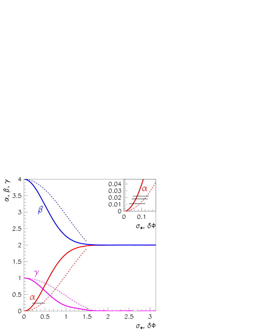
Figure 2: The coefficients $\alpha$, $\beta$ and $\gamma$ as functions of $\sigma_{\Phi}$ in case A (solid lines) and as functions of $\delta\Phi$ in case B (dashed lines). A horizontal line in the lower left corner indicates the value of $\alpha$ in $pp$ collisions at RHIC energy, $\sqrt{s}=200$ GeV. In the upper right a magnified view of the small $\alpha$ region is given. The horizontal lines indicate the values of $\alpha$ at ISR energies (see Section 3 and Table 1).

The effect of these fluctuations (randomization) at the parton collision level will be superimposed on the intrinsic transverse momentum of partons expressed by $\sigma_{k}$. Furthermore, hadronization (jet fragmentation) will complicate the picture. We incorporate the consequences of hadronization gradually: in a first step, in Section 3, the momentum fraction of the trigger hadron is taken into account. Section 4 contains a more detailed discussion.

3 Partial correlations at ISR and RHIC energies

Data on di-hadron correlations in $pp$ collisions at ISR energies $\sqrt{s}=31,\ 45,\ 62$ GeV [7] and at RHIC energies $\sqrt{s}=200$ GeV [1, 9] show a dependence on the transverse momentum of the trigger hadron $p_{T,trig}$, which is at this point in our treatment represented by $p_{T1}$. Figure 3 displays available $pp$ data at ISR and RHIC.

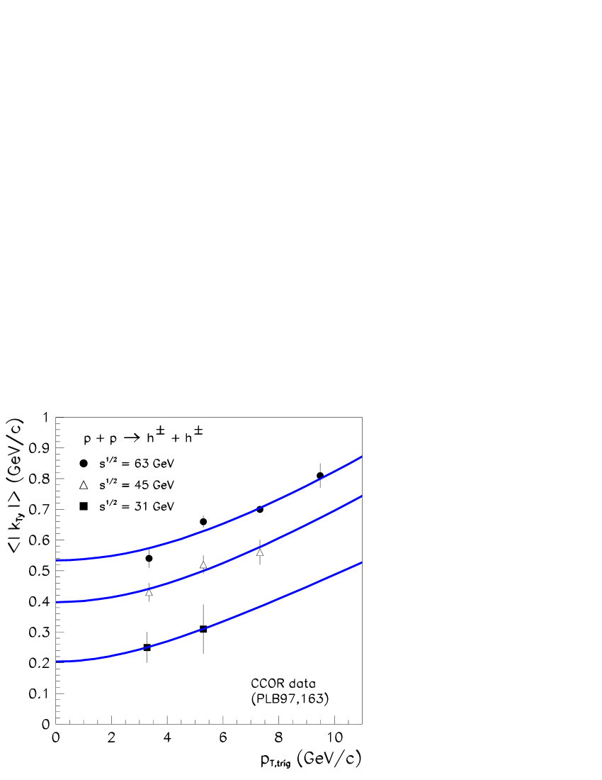
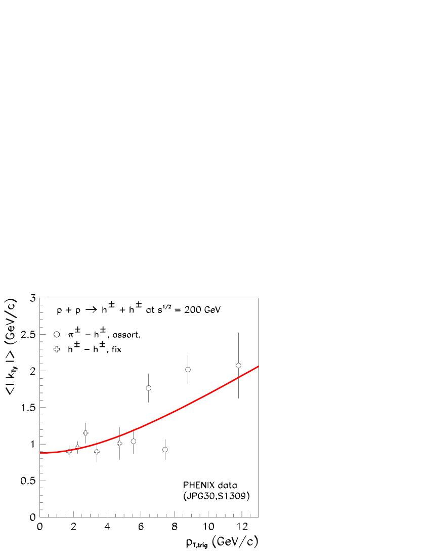
Figure 3: Data published for hadron-hadron correlations in $pp$ collisions at ISR [7] (left panel) and RHIC [9] (right panel) together with the fit for a partially correlated parton system (see text and Table 1.).

Since the parton-level quantity $\langle|k_{Ty}|\rangle=\sqrt{(\langle(p_{T2}\sin(\Phi_{2}-\Phi_{1}))^{2}\rangle)/\pi}$ is independent of $p_{T1}$ in a strongly correlated system (see eq.(8)), the $p_{T1}$ dependence on Fig. 3 indicates a partially correlated situation at ISR and RHIC (see eq.(17)):

$$\langle|k_{Ty}|\rangle=\frac{1}{\sqrt{\pi}}\sqrt{\langle(p_{T2}\sin(\Phi_{2}-\Phi_{1}))^{2}\rangle_{pc}}=\frac{1}{\sqrt{\pi}}\sqrt{\frac{\alpha}{4}p^{2}_{T1}+2\cdot\sigma^{2}_{k}}\,\,,$$ (19)

meaning that the intrinsic width $\sigma_{k}$ can be identified as the limiting value when $p_{T,trig}\rightarrow 0$.

This expression is valid if parton fragmentation is neglected. To include fragmentation effects at this stage we use a simple prescription to take into account that the experimentally measured trigger hadron carries a fraction of the corresponding parton transverse momentum, and we correct with the mean momentum fraction carried by the produced hadron,

$$p_{T,trig}=z\cdot p_{T1}\,\,\,.$$ (20)

Thus, in terms of hadronic variables the expression (19) takes the following form:

$$\langle|k_{Ty}|\rangle=\frac{1}{\sqrt{\pi}}\sqrt{\frac{\alpha}{4z^{2}}p^{2}_{T,trig}+2\cdot\sigma^{2}_{k}}\,\,.$$ (21)

Eq. (21) can be compared to existing experimental data. For RHIC energy the fragmentation correction is $\langle z\rangle_{p_{T}>{\textrm{3\ GeV}}}=0.75\pm 0.05$ [9, 19]. For ISR data we use $\langle z\rangle\approx 0.85$ [7, 9]. Since $\langle z\rangle$ is independent of $p_{T,trig}$ [9], it can be easily included in eq. (21) by rescaling $\alpha$. Figure 3 shows the best fit according to eq. (21). Table 1 summarizes the parameters of the fit.

Table 1: Extracted correlation coefficient, $\alpha$, and the width of the initial parton transverse momentum distribution, $2\sigma^{2}_{k}$, at ISR and RHIC energies in $pp$ collisions.

$\sqrt{s}_{pp}$ (GeV)	$\langle z\rangle$	$\alpha$	$2~{}\sigma^{2}_{k}$ (GeV2)
31	0.85	0.011	0.13
45	0.85	0.018	0.50
62	0.85	0.022	0.90
200	0.75	0.240	2.42

It is of interest to remark here that the obtained width at RHIC energy matches closely the value used in a transverse-momentum augmented perturbative QCD calculation in $pp$ collisions in Ref. [20]: $2\,\sigma_{k}^{2}=2.5$ GeV². As discussed earlier, this value contains the effect of initial soft gluon radiation. In nuclear collisions ($dAu$ and $AuAu$), the widths $\sigma_{k}$ can be different, in which case $2\,\sigma_{k}^{2}\rightarrow\sigma_{k1}^{2}+\sigma_{k2}^{2}$.

However, parton fragmentation has a more complicated effect on the relation between measurable quantities and parton transverse momenta than reflected in eq. (20). Next we examine to what extent the results in Table 1 and Fig. 3 remain valid in a more realistic treatment of hadronization.

4 Hadron-hadron correlations in $pp$ collisions

In a real $pp$ experiment, of course, hadron-hadron correlations are measured. This introduces several complications in the evaluation of correlations and of parton intrinsic transverse momenta. Fragmentation of the secondary partons produces a distribution of outgoing hadrons. The experiments pick a trigger hadron with transverse momentum $p_{T,trig}$ and an associated hadron with transverse momentum $p_{T,assoc}$ from the measured distribution. The azimuthal correlation function displays a two-peak structure, where the width of the near-side peak is denoted by $\sigma_{N}$ and the width of the away-side peak is $\sigma_{A}$. The value of $\sigma_{N}$ carries information on the fragmentation process only, while $\sigma_{A}$ may contain the contribution of the intrinsic transverse momentum. In a fully randomized situation all information about intrinsic $k_{T}$ is lost (see eq.(12)) and we would expect $\sigma_{A}\approx\sigma_{N}$. However, measurements show $\sigma_{A}>\sigma_{N}$, indicating that the width of the intrinsic transverse momentum distribution can be extracted from hadron-hadron correlations.

Figure 4: Schematic view of the near side (left panel) and away side (right panel) correlations with parton fragmentation and notation for angles (see text).

4.1 Near-side correlation and parton fragmentation

Data from RHIC show that in $pp$ and $dAu$ collisions the widths of the near-side peaks, $\sigma_{N}$, are in good agreement [9, 10]. An average value for the transverse momentum component of the trigger hadron relative to the jet axis, $\langle|j_{Ty}|\rangle=324\pm 6$ MeV/c has been obtained in the usual notation [14]. This value agrees within error bar with the $AuAu$ value at RHIC, independent of centrality [9], which indicates a collision-system independent fragmentation. Furthermore, the data are close to the ISR value for $pp$ collisions, $\langle|j_{Ty}|\rangle=393\pm 3$ MeV/c [7]. These results suggest the existence of an approximately universal fragmentation pattern, almost independent of energy, centrality and collision system.

Here we summarize the assumptions needed to obtain an expression for the near-side azimuthal correlation. Figure 4 (left side) illustrates parton fragmentation and the definition of the quantities necessary to extract the near-side correlation.

In near-side correlations, the trigger hadron and the associated hadron both arise from the same parton and the following relation holds: $\sin\Delta\phi_{N}=\sin(\phi_{tj}+\phi_{aj})$. In light of our analysis in previous Sections, we calculate $\langle p_{out,N}^{2}\rangle=\langle(p_{T,assoc}\sin\Delta\phi_{N})^{2}\rangle$. Since fragmentation angles $\phi_{tj}$ and $\phi_{aj}$ are statistically independent, we obtain the following expression for averaged azimuths, where the cross terms have been dropped (since they average to zero):

$$\langle{p^{2}_{out,N}}\rangle=\langle p_{T,assoc}^{2}\sin^{2}\Delta\phi_{N}\rangle=\langle p_{T,assoc}^{2}\sin^{2}\phi_{tj}\cdot\cos^{2}\phi_{aj}\rangle+\langle p_{T,assoc}^{2}\cos^{2}\phi_{tj}\cdot\sin^{2}\phi_{aj}\rangle.$$ (22)

Following the notation of Fig. 4, introducing $x_{h}=p_{T,assoc}/p_{T,trig}\,$, and substituting the azimuths in eq. (22):

$$\langle p^{2}_{out,N}\rangle = \left\langle j^{2}_{Ty,trig}\,x_{h}^{2}\,\left(1-\frac{j^{2}_{Ty,assoc}}{p^{2}_{T,assoc}}\right)\right\rangle+\left\langle\left(1-\frac{j^{2}_{Ty,trig}}{p^{2}_{T,trig}}\right)j^{2}_{Ty,assoc}\right\rangle\,.$$ (23)

For $p_{T,trig},\ p_{T,assoc}\geq 2$ GeV we can neglect the terms $j^{2}_{Ty,assoc}/p^{2}_{T,assoc}\sim{\cal O}(0.05)$ and $j^{2}_{Ty,trig}/p^{2}_{T,trig}\sim{\cal O}(0.05)$, generating a 10 % uncertainty in the results. Eq. (23) simplifies to

$$\left\langle p^{2}_{out,N}\right\rangle=\langle j^{2}_{Ty,trig}\,x^{2}_{h}\rangle+\langle j^{2}_{Ty,assoc}\rangle\ .$$ (24)

Assuming a universal fragmentation pattern characterized by $\langle j^{2}_{Ty}\rangle\equiv\langle j^{2}_{Ty,assoc}\rangle\approx\langle j^{2}_{Ty,trig}\rangle$ and $x_{h}$ independence, one gets

$$\left\langle p^{2}_{out,N}\right\rangle=\langle j^{2}_{Ty}\rangle\cdot(1+\langle x^{2}_{h}\rangle)\ .$$ (25)

In a final step we connect $\left\langle p^{2}_{out,N}\right\rangle$ to the measured width of the near side azimuthal correlation. Assuming a Gaussian distribution and following the usual procedure [10], one can approximate $\left\langle p^{2}_{out,N}\right\rangle$ within 10 % precision with the following expression:

$$\langle p^{2}_{out,N}\rangle \approx \left\{\begin{array}[]{lll}\langle p^{2}_{T,assoc}\rangle\ \sigma^{2}_{N}&&\mbox{\rm if \hskip 11.38092pt $\Delta\phi_{N}\in[0,\pi/8]$}\\ \langle p^{2}_{T,assoc}\rangle[\sin\sigma_{N}^{2}-\sigma_{N}^{4}]&&\mbox{\rm if \hskip 11.38092pt $\Delta\phi_{N}\in\left[\pi/8,\pi/5\right]$}\end{array}\right.\,\,\,.$$ (28)

Experimental data for the near side correlation at ISR and RHIC energies [7, 9] allow us to apply the approximation in the top line of eq. (28). Since in two-dimensional averaging for any quantity $X$ we have $\langle|X|\rangle^{2}=2/\pi\cdot\langle X^{2}\rangle$, one can simplify eq.(25) and obtain the usual form [7, 9, 10] for the fragmentation broadening:

$$\langle|j_{Ty}|\rangle=\frac{\sqrt{2\langle p^{2}_{T,assoc}\rangle}}{\sqrt{\pi}}\ \frac{\sigma_{N}}{\sqrt{1+\langle x_{h}^{2}\rangle}}$$ (29)

This can be evaluated from data on $p_{T,assoc}$, $p_{T,trig}$ and the near-side azimuthal width $\sigma_{N}$. The result for $\langle|j_{Ty}|\rangle$ does not depend on $p_{T,trig}$ directly, the only dependence comes through the quantity $x_{h}$. We are now in a position to investigate the away-side correlation and its relation to the intrinsic transverse momentum.

4.2 Away-side correlation and intrinsic transverse momentum

Away-side hadron correlations carry information on the intrinsic transverse momentum of partons. Fig. 4 (right side) displays the geometry of this correlation. Here, the trigger hadron and the associated hadron originate in different partons characterized by different transverse momenta ${\bf p}_{T1}$ and ${\bf p}_{T2}$, respectively. We choose ${\bf p}_{T1}$ to be the transverse momentum of the parton which will give birth to the trigger hadron with momentum ${\bf p}_{T,trig}$.

We need to evaluate the expectation value of $p^{2}_{out,A}=p^{2}_{T,assoc}\sin^{2}\Delta\phi_{A}$ to determine the away-side azimuthal correlation. One can read off of Fig. 4 (right side) that $\Delta\phi_{A}=\phi_{tj}+\Phi_{21}+\phi_{aj}$, where $\Phi_{21}=\Phi_{2}-\Phi_{1}$. All cross terms drop in the averaging, since fragmentation and initial kinematics, and fragmentation of trigger and associated hadrons are independent.

Now one can express the wanted $\langle p^{2}_{out,A}\rangle$ as

$$\langle p^{2}_{out,A}\rangle = \langle p^{2}_{T,assoc}\sin^{2}(\phi_{tj}+\Phi_{21}+\phi_{aj})\rangle=$$ (30)

$$= \langle p^{2}_{T,assoc}(1-\sin^{2}\Phi_{21})\ (\sin^{2}\phi_{tj}\cos^{2}\phi_{aj}+\cos^{2}\phi_{tj}\sin^{2}\phi_{aj})\rangle+$$

$$+\langle p^{2}_{T,assoc}\sin^{2}\Phi_{21}\ (1-\sin^{2}\phi_{tj}\cos^{2}\phi_{aj}-\cos^{2}\phi_{tj}\sin^{2}\phi_{aj})\rangle\,.$$

Taking advantage of the independence of fragmentation and initial kinematics once again, we can separate the expectation values of the azimuths and apply eq. (22) and the approximation in the top line of eq. (28) for the fragmentation process:

$$\langle p^{2}_{out,A}\rangle = (\langle p^{2}_{T,assoc}\rangle-\langle p^{2}_{T,assoc}\sin^{2}\Phi_{21}\rangle)\,\sigma_{N}+\langle p^{2}_{T,assoc}\sin^{2}\Phi_{21}\rangle\left(1-\sigma^{2}_{N}\right)$$ (31)

$$= \langle p^{2}_{T,assoc}\rangle\,\sigma_{N}+\langle p^{2}_{T,assoc}\sin^{2}\Phi_{21}\rangle\left(1-2\sigma^{2}_{N}\right)\,\,\,.$$

Here we recognize that $\langle p^{2}_{T,assoc}\sin^{2}\Phi_{21}\rangle$ is related to the intrinsic $k_{T}$ of the colliding partons in the incoming protons, as discussed in Section 2. Recall that $p_{T2}$ and $\Phi_{21}$ are not independent, and we wish to use eq. (17) to implement a partially correlated situation. We express the corresponding term from eq. (31):

$${\langle p^{2}_{T,assoc}\sin^{2}\Phi_{21}\rangle} = \frac{\langle p^{2}_{T,assoc}\rangle\,(\sigma^{2}_{A}-\sigma^{2}_{N})}{1-2\sigma^{2}_{N}}\,\,\,.$$ (32)

For simplicity we applied the top line of eq. (28) to connect the away-side angular correlation (characterized by the width $\sigma_{A}$) with the quantity $\langle p^{2}_{out,A}\rangle$. At larger values of $\sigma_{A}$ the approximation in the bottom line of eq. (28) leads to a more precise expression. Further approximations are also available in the literature [9, 10, 11].

In order to capture the correlation properties of the left-hand side we need to return to parton level. To separate the fragmentation effects for the associated hadron we take into account that

$$p_{T,assoc}\cdot\cos\phi_{aj} = z_{assoc}\cdot p_{T2}\,\,\,.$$ (33)

Utilizing the angular features of fragmentation we take expectation values separately, except for $p^{2}_{T2}\sin^{2}\Phi_{21}$ as discussed above,

$$\langle p^{2}_{T,assoc}\sin^{2}\Phi_{21}\rangle=\frac{\langle z_{assoc}\rangle^{2}}{\langle\cos^{2}\phi_{aj}\rangle}\ \langle p^{2}_{T2}\sin^{2}\Phi_{21}\rangle\,\,\,.$$ (34)

The last term on the right-hand side of eq.(34) reminds us of eq. (17) for a partially correlated situation with a dependence on a parton-level $p_{T1}$. To express this with the transverse momentum of the trigger hadron (see Fig. 4) we use (compare eq. (20))

$$p_{T,trig}\cdot\cos\phi_{tj} = z_{trig}\cdot p_{T1}\,\,\,.$$ (35)

Combining eqs.(17), (32), (34), and (35), we obtain

$$\frac{\sigma^{2}_{A}-\sigma^{2}_{N}}{1-2\ \sigma^{2}_{N}} = \frac{\langle z_{assoc}\rangle^{2}}{\langle\cos^{2}\phi_{aj}\rangle\ \langle p^{2}_{T,assoc}\rangle}\left[\frac{\alpha}{4}p^{2}_{T1}+2\cdot\sigma^{2}_{k}\right]=$$ (36)

$$= \frac{\langle z_{assoc}\rangle^{2}}{\langle\cos^{2}\phi_{aj}\rangle\ \langle p^{2}_{T,assoc}\rangle}\left[\frac{\alpha}{4}\frac{\langle\cos^{2}\phi_{tj}\rangle}{\langle z_{trig}\rangle^{2}}p^{2}_{T,trig}+2\cdot\sigma^{2}_{k}\right]\,\,\,.$$

If the azimuthal angles $\phi_{tj}$ and $\phi_{aj}$ are independent and uncorrelated, then $\langle\cos^{2}\phi_{tj}\rangle=\langle\cos^{2}\phi_{aj}\rangle=1/2$. In this case we get

$$\frac{\sigma^{2}_{A}-\sigma^{2}_{N}}{1-2\ \sigma^{2}_{N}} = \frac{2\langle z_{assoc}\rangle^{2}}{\langle p^{2}_{T,assoc}\rangle}\left[\frac{\alpha\,p^{2}_{T,trig}}{8\langle z_{trig}\rangle^{2}}+2\sigma^{2}_{k}\right]\,\,\,.$$ (37)

The message of this expression is that at a given $p_{T,trig}$, measuring $\sigma_{A}$ and $\sigma_{N}$ in a $p_{T,assoc}$ window, and estimating $\langle z_{assoc}\rangle$, one can read off $\sigma_{k}$ from the small $p_{T,trig}$ behavior of the combination on the left-hand side, as the limit $p_{T,trig}\rightarrow 0$. In that limit the wanted parton-level averaged transverse momentum is

$$\langle|k_{Ty}|\rangle\equiv\sqrt{\frac{2\sigma_{k}^{2}}{\pi}}=\frac{\sqrt{\langle p^{2}_{T,assoc}\rangle}}{\sqrt{\pi}\,\langle z_{assoc}\rangle}\sqrt{\frac{\sigma^{2}_{A}-\sigma^{2}_{N}}{1-2\ \sigma^{2}_{N}}}\,\,\,.$$ (38)

We propose that the data on near and away-side correlations be evaluated in this manner. The denominator $(1-2\sigma_{N}^{2})$ will not approach zero according to available data [21], but may be important numerically. On the other hand, the data [21] suggest, that the application of a more precise approximation for the away side width (see the discussion around eq. (28)) may be warranted [9, 10, 11].

5 Summary

We have shown in this paper that no information can be recovered on the initial intrinsic transverse momentum distribution of partons in the proton if the transverse momenta of the outgoing partons are fully randomized. However, proton-proton collisions display partial randomization in the transverse plane, offering the opportunity to extract the width of the intrinsic-$k_{T}$ distribution from di-hadron correlations. We have found $p_{T,trig}$-dependent correlations at ISR and RHIC energies, where the intrinsic-$k_{T}$ widths can be extracted in the limit $p_{T,trig}\rightarrow 0$. This procedure survives the complications introduced by fragmentation and we propose a method to obtain the wanted initial width from hadron-hadron correlations using the widths of the near and away-side peaks of the hadron-hadron correlation functions.

At fix $p_{T,trig}$ the dependence of $\langle|k_{Ty}|\rangle$ on $p_{T,assoc}$ displayed in this paper, especially eq.(38), provides a new insight for recent experimental analyses (see e.g. Ref. [21, 22]). In particular, the denominator $(1-2\sigma_{N}^{2})$ can be important in eq.(38). The interplay between $\langle p^{2}_{T,assoc}\rangle$ and $\langle z\rangle$ at high $p_{T}$ requires further study.

The present discussion was restricted to proton-proton collisions. The generalization for nuclear collisions will include $k_{T}$-broadening from multiple scattering and possibly unequal widths when the colliding nuclei are of different species. As mentioned above, in $dAu$ (and $AuAu$) collisions more final-state interactions of the outgoing partons are expected. Therefore, a difference in the variation of the $p_{T,trig}$ dependence of $\langle|k_{Ty}|\rangle$ between $pp$ and $dAu$ reactions could provide an alternative way to separate initial and final-state interactions of partons. So far, the extracted widths from $dAu$ collisions are very similar to the $pp$ values at RHIC energy, but more detailed experiments and analyses may refine the situation. In addition, we expect that the $k_{T}$-widths used to describe single-particle spectra and the ones extracted from hadron-hadron correlations can be brought into complete accord along these lines.

References

-
[1]
M. Chiu et al. (PHENIX Coll.),
Nucl. Phys. A715, 761c (2003);
N.N. Ajitanand et al. (PHENIX Coll.), Nucl. Phys. A715, 765c (2003). -
[2]
C. Adler et al. (STAR Coll.), Phys. Rev. Lett. 90,
082302 (2003);
D. Hardtke et al. (STAR Coll.), Nucl. Phys. A715, 801c (2003). - [3] M. Gyulassy, P. Lévai, and I. Vitev, Nucl. Phys. B571, 197 (2000); Phys. Rev. Lett. 85, 5535 (2000); Nucl. Phys. B594, 371 (2001); Phys. Lett. B538, 282 (2002).
- [4] G. Fai et al., JHEP (2001), PrHEP2001/242, (hep-ph/0111211).
- [5] R. Baier, Y.L. Dokshitzer, A.H. Mueller, S. Peigne, and D. Schiff, Nucl. Phys. B483, 291 (1997); ibid. B531, 403 (1998); B.G. Zakharov, JETP Lett. 63, 952 (1996).
- [6] M. Gyulassy, I. Vitev, X.N. Wang, B.W. Zhang, nucl-th/0302077.
- [7] A.L.S. Angelis, et al. (CCOR Coll.), Phys. Lett. B97, 163 (1980).
- [8] M.D. Corcoran et al. (E609 Coll.), Phys. Lett. B 259, 209 (1991).
- [9] J. Rak, et al. (PHENIX Coll.), J. Phys. G30, S1309 (2004).
- [10] J. Jia, J. Phys. G31, S521 (2005).
- [11] J. Qiu, I Vitev, Phys. Lett. B570, 161 (2003).
- [12] D. Boer, W. Vogelsang, Phys. Rev. D69, 094025 (2004).
- [13] I. Vitev, hep-ph/0501255
- [14] We continue to use the notation and for the component of the transverse vectors perpendicular to the direction of the jet axis and for transverse vectors perpendicular to the trigger direction (see Fig. 4 and Refs [9, 10]).
- [15] R.D. Field, Application of Perturbative QCD (Addison-Wesley, Reading, MA, 1995).
- [16] C.Y. Wong and H. Wang, Phys. Rev. C58, 376 (1998).
- [17] X.N. Wang, Phys. Rev. C61, 064910 (2001).
- [18] Y. Zhang, G. Fai, G. Papp, G.G. Barnaföldi, and P. Lévai, Phys. Rev. C65, 034903 (2002).
- [19] X.F. Zhang, G. Fai, P. Lévai, Phys. Rev. Lett. 89, 272301 (2002).
- [20] P. Lévai, G. Papp, G.G. Barnaföldi, G. Fai, nucl-th/0306019.
- [21] J. Rak, Talk at DNP Fall 2004 Meeting, Chicago, IL.
- [22] J. Jia, Talk at DNP Fall 2004 Meeting, Chicago, IL.