Mixing of Pentaquark and Molecular States

Abstract

There are experimental evidences for the existence of narrow states $\Theta^{+}$ and $\Theta_{c}$ with the same quantum numbers of $uudd\bar{s}$ and $uudd\bar{c}$ pentaquarks and also $NK^{(*)}$ and $ND^{(*)}$ molecular states. Their masses deviate from many theoretical estimates of the pure pentaquark and molecular states. In this work we study the possibility that the observed $\Theta^{+}$ and $\Theta_{c}$ are mixtures of pure pentaquark and molecular states. The mixing parameters are in general related to non-perturbative QCD which are not calculable at present. We determine them by fitting data from known states and then generalize the mechanism to $\Theta_{b}$ to predict its mass and width. The mixing mechanism can also naturally explain the narrow width for $\Theta^{+}$ and $\Theta_{c}$ through destructive interferences, even if the pure pentaquark and molecular states have much larger decay widths. We also briefly discuss the properties of the partner eigenstates of $\Theta^{+}$ and $\Theta_{c}$ and the possibility of experimentally observe them. Moreover, probable consequences of multi-state mixing are also addressed.

I Introduction

Following the discovery of $\Theta^{+}$ by the LEPS collaboration leps , some experimental collaborations diana ; clasa ; clasb ; saphir ; itep ; hermes ; itep-2 ; zeus ; cosy-tof ; togoo ; aslanyan ; nakano ; troyan have also confirmed its existence. Its mass is $1539.2\pm 1.6$ MeV with a very narrow width of $0.9\pm 0.30$ MeV. The $\Theta^{+}$ is a baryon state with exotic strangeness quantum number $S=+1$ which cannot be understood as a normal baryon made of three quarks. It is reasonable to interpret $\Theta^{+}$ as a pentaquark $(uudd\bar{s})$ which was predicted in several theoretical worksPredict . Recently the H1 Collaboration reported their finding of a new narrow resonance H1 , whose mass and width are $3099\pm 3(stat)\pm 5(syst)$ MeV and $12\pm 3$ MeV, respectively. This narrow resonance can be interpreted as a charmed pentaquark $\Theta_{c}$ ($uudd\bar{c}$) which has also been studied theoretically beforelipkin . There is also the possibility of the existence of a new state $\Theta_{b}$ with the $\bar{c}$ replaced by a $\bar{b}$ in $\Theta_{c}$. Even though it has not been observed at present, future experiments will provide more information. One should also note that there are other experiments which do not observe the $\Theta^{+}$ and $\Theta_{c}$jinshan states. More investigations are needed to confirm the existence of these states.

There have been extensive studies for light pentaquark and multi-quark stateslight ; width ; Lipkin1 ; Kingman Cheung , and as well as heavy pentquarksheavy ; Lipkin2 ; Jaffe ; Kingman Cheung . One of the attractions of investigating pentaquarks is that one may gain more knowledge on not only the hadron structure, but also insights to the underlying mechanism which binds quarks into a multi-body system. It is interesting to investigate if there exist sub-structures in the five-constituent systems. Karliner and Lipkin Lipkin1 ; Lipkin2 suggested that the $\Theta^{+}$ has a diquark-triquark $(ud)$-$(ud\bar{s})$ sub-structure, and on the other hand, Jaffe and Wilczek (JW) Jaffe proposed that $\Theta^{+}$ is a bound state of an antiquark with two highly correlated spin-zero $ud$ diquarks, moreover they also suggested a mixing of an octet and an antidecuplet which is recently re-studied Tetsuo . In these frameworks $\Theta^{+}$ is a $1/2^{+}$ particle. The predictions on the central value of $\Theta^{+}$ mass spread fromLipkin1 ; Lipkin2 ; Jaffe ; Kingman Cheung 1481 MeV to 1592 NeV and the range covers the central value of the data. The predictions on the $\Theta_{c}$ mass is in the range of 2710 MeV to 2997 MeV which is consistently below the central value 3099 MeV of the data. The mass of $\Theta_{b}$, using the same method, is predicted to be in the range of 6050 MeV to 6422 MeV. There are also several lattice calculations for the masses of the pentqaurkslattice ; chiu ; chiu1 and so far, no conclusive results about the $\Theta^{+}$ mass and its parity have been achieved. For $\Theta_{c}$ with positive parity the mass is estimated to be $2977\pm 109$ MeV in Ref. chiu . At present, theoretical estimates have large uncertainties and it is entirely possible that a pure pentaquark state mass fits the reported mass of $\Theta_{c}$ from H1. For the pentaquark decay width, the situation is even more uncertainwidth ; Lipkin1 ; Lipkin2 ; Kingman Cheung . The present theory is in a very unsatisfactory situation.

There were also attempts to identify $\Theta^{+}$ as a $N$-$K$ molecular state. However theoretical calculationsJaffe ; molecular typically give much larger width and lower mass for the molecular state compared with the data. There is also a possibility that the molecular state is a $N$-$K^{*}$ molecular state. In this case the mass is above the measured $\Theta^{+}$ mass, namely a typical negative binding energy of $N$-$K^{*}$ cannot reduce the total mass to the data. For this reason, molecular states cannot be identified as the observed $\Theta^{+}$. However these states correspond to a different component in the Hilbert space, although the triquark-diquark, or diquark-diquark-antiquark pentaquark combinations and the molecular states have different color structures, the pentaquark and the moldecular states may mix because they all have the same overall quantum numbers. It is clear that no mixing would be needed if the observed states could be identified with pure pentaquark or molecular states.

There are interesting consequences if mixing indeed exists. Consider a mixing of two states, a pure pentaquark state mixes with a molecular state. One notes that when diagonalizing a two-by-two mass matrix, one obtains two eigenvalues with one of them being smaller than the minimum of the original two diagonal matrix elements and another larger than the maximum if the mixing is non-zero. One of the eigenstates is identified with the observed $\Theta$ state and another is a physical partner state. Because mixing, one can expect a mixed state possesses a mass which is consistent with data, while the predicted pure pentaquark and the pure molecular $N$-$D$ (or $N$-$D^{*}$) state have masses which are different than the observed $\Theta$ state. This motivates us to consider the possibility that the observed $\Theta^{+}$ and $\Theta_{c}$ may be mixtures of pure pentaquark and molecular states. Another challenging property of $\Theta^{+}$ and $\Theta_{c}$ is their narrow widths. We will show that even if both the pure pentaquark and molecular states may have larger widths, but a destructive interference between them may result in overall narrow widths for the observed resonances.

Similar idea in obtaining a narrow width for other systems was discussed in ref-n and some authors suggested that the smallness of the width of $\Theta^{+}$ may be due to a so-called “super-radiance” which actually is also a destructive interference effectAuerbach .

Although at this stage the indication of mixing is not strong, nevertheless it is interesting to see what this will lead to. In this work we study some consequences of pure pentaquark and molecular states mixing for $\Theta^{+}$, $\Theta_{c}$ and $\Theta_{b}$. Our strategy is as the following. We first calculate the mass of the $N$-$K$ ($N$-$K^{*}$)molecular state (having the same quantum number as $\Theta^{+}$) by using linear $\sigma-$model and taking a theoretical prediction for the pure pentaaquark $\Theta^{+}$ mass as input for the mixing mass matrix. We phenomenologically introduce a mixing parameter in the two-state mass matrix, and diagonalize the mass matrix to obtain new eigenvalues and eigenstates. By fitting data, we determine the mixing parameter with which we evaluate the total width of the corresponding eigenstate.

Indeed, our discussions cannot offer explanations for large mixing between a pentaquark and a molecular state which requires a good understanding of non-perturbative QCD effects. We will stay at the phenomenological level to study the consequences. More accurate experimental measurements and lattice QCD calculations on properties of the resonances may provide some clues to this problem.

We then carry out calculations for $\Theta_{c}$ with the same strategy and determine the corresponding mixing parameter by fitting data. Because charm quark is much heavier than strange quark, one cannot expect the mixing parameters in the cases for $\Theta^{+}$ and $\Theta_{c}$ to have any direct relation. However, bottom and charm quarks all are supposed to be heavy compared with the QCD scale, thus there may be a connection between the parameters for $\Theta_{c}$ and $\Theta_{b}$. By a simple argument based on one gluon exchange picture we relate the parameters for $\Theta_{b}$ to those of $\Theta_{c}$. Using this value, we estimate the mass and width for $\Theta_{b}$.

Obviously there could be multi-state mixing among pentaquark and molecular states of N-P and N-V types. By adjusting parameters (there are more of them than in the two-state mixing), the measured values can be re-produced. If none of the pure states has a mass closer to the observed pentaquark states, the mixing parameters need to be large. This is the case we are interested in. Using model calculations based on one particle ((pseudo)scalar or vector meson) exchange, we find that mixing between N-P and N-V states is considerably smaller than the mixing parameter of pentaquark with either P-N or V-N which is obtained by fitting data. We therefore will only concentrate on the mixing between the pentaquark and molecular states. We will analyze the simple two-state mixing case in details, and then will discuss the possible multi-state mixing.

This paper is organized as follows, after the introduction, in section II, we derive the formulation for the mixed states where we only concentrate on the cases of two-state mixing. In Section III, we present our numerical results for two-state mixing, and in Section IV, we discuss possible consequences of three-state mixing and use several figures to illustrate the changes of the spectra from the two-state mixing case. And finally in section V, we discuss some implications and draw our conclusions.

II Pentaquark and Molecular State Mixing

II.1 Effective Potential of Molecular State

We postulate that the molecular state only contains two constituents. The concerned molecular states can be categorized into $V$-$N$ and $P$-$N$ systems where $V$ and $P$ correspond to a vector and a pseudoscalar meon, respectively. Thus, the molecular state can be $KN$ or $K^{*}N$ for $\Theta^{+}$, $DN$ or $D^{*}N$ for $\Theta_{c}$, and $BN$ or $B^{*}N$ for $\Theta_{b}$. The more complicated structures with three or more constituents will be commented on later.

We use the traditional method landaue by assuming the potential between a nucleon and a meson to be due to one particle exchange which may be a scalar, a pseudoscalar, or a vector meson, and neglecting other heavier and multi-particle intermediate states. In the linear $\sigma$-model, the effective Lagrangian relevant to a $\sigma$, a $\pi$ and a $\rho$ exchange is given byGeogi ; lin ; Gokalp ; Pir ; Bramon ; Barry

$$L = g\bar{\psi}(\sigma+i\gamma_{5}{\mbox{\boldmath$\tau$}}\cdot{\mbox{\boldmath$\pi$}})\psi+g_{{}_{NN}\rho}\bar{\psi}\gamma_{\mu}{\mbox{\boldmath$\tau$}}\psi\cdot{\mbox{\boldmath$\rho$}}^{\mu}+g_{PP\sigma}P^{\dagger}P\mathbf{\sigma}+g_{PP\rho}(P^{\dagger}{\mbox{\boldmath$\tau$}}\partial_{\mu}P-\partial_{\mu}P^{\dagger}{\mbox{\boldmath$\tau$}}P)\cdot{\mbox{\boldmath$\rho$}}^{\mu}$$

$$+g_{VV\pi}\varepsilon^{\mu\nu\alpha\beta}\partial_{\mu}V^{\dagger}_{\nu}{\mbox{\boldmath$\tau$}}\partial_{\alpha}V_{\beta}\cdot{\mbox{\boldmath$\pi$}}+g_{VV\sigma}[\partial^{\mu}{V^{\dagger}}^{\nu}\partial_{\mu}V_{\nu}-\partial^{\mu}{V^{\dagger}}^{\nu}\partial_{\nu}V_{\mu}]\sigma+g_{VV\rho}[(\partial_{\mu}{V^{\dagger}}^{\nu}{\mbox{\boldmath$\tau$}}V_{\nu}$$

$$-{V^{\dagger}}^{\nu}{\mbox{\boldmath$\tau$}}\partial_{\mu}V_{\nu})\cdot{\mbox{\boldmath$\rho$}}^{\mu}+({V^{\dagger}}^{\nu}{\mbox{\boldmath$\tau$}}\cdot\partial_{\mu}{\mbox{\boldmath$\rho$}}_{\nu}-\partial_{\mu}{V^{\dagger}}^{\nu}{\mbox{\boldmath$\tau$}}\cdot{\mbox{\boldmath$\rho$}}_{\nu})V^{\mu}+{V^{\dagger}}^{\mu}({\mbox{\boldmath$\tau$}}\cdot{\mbox{\boldmath$\rho$}}^{\nu}\partial_{\mu}V_{\nu}-{\mbox{\boldmath$\tau$}}\cdot\partial_{\mu}{\mbox{\boldmath$\rho$}}^{\nu}V_{\nu})]$$

$$+[g_{VP\pi}{V^{\dagger}}^{\mu}{\mbox{\boldmath$\tau$}}\cdot(P\partial_{\mu}{\mbox{\boldmath$\pi$}}-\partial_{\mu}P{\mbox{\boldmath$\pi$}})+h.c.]+g_{VP\rho}\varepsilon^{\mu\nu\alpha\beta}[\partial_{\mu}{\mbox{\boldmath$\rho$}}_{\nu}\partial_{\alpha}V^{\dagger}_{\beta}\cdot{\mbox{\boldmath$\tau$}}P+\partial_{\mu}V^{\dagger}_{\nu}{\mbox{\boldmath$\tau$}}\cdot\partial_{\alpha}{\mbox{\boldmath$\rho$}}_{\beta}P],$$

where $P,V$ are an iso-spin doublet psudoscalar and vector mesons, i.e. $((K^{+})^{(*)},(K^{0})^{(*)})^{T}$, $((D^{+})^{(*)},(D^{0})^{(*)})^{T}$, $((B^{+})^{(*)},(B^{0})^{(*)})^{T}$ and their charge-conjugates. In this expression, we only keep the concerned terms of the chiral Lagrangian for later calculations.

In analog to the treatment with the chiral Lagrangian, in this work all the coefficients at the effective vertices are derived by fitting data of certain physical processes, where all external particles are supposed to be on their mass-shells. Meanwhile, we introduce form factors to compensate the off-shell effects of the exchanged meson. At each vertex, the form factor is parameterized as form factor

$$\frac{\Lambda^{2}-M_{m}^{2}}{\Lambda^{2}-q^{2}}$$ (2)

where $\Lambda$ is a phenomenological parameter. If the exchanged particle is on-shell $q^{2}=M^{2}_{m}$, the form factor is unity.

To derive an effective potential, we set $q_{0}=0$ and write down the elastic scattering amplitude in the momentum space and then carry out a Fourier transformation turning the amplitude into an effective potential in the configuration space. The total effective potential for P-N system is the sum of contributions of $\sigma$ and $\rho$:

$$V_{eff}^{\mathbf{P}-N}(r)=V_{\sigma}^{\mathbf{P}-N}(r)+V_{\rho}^{\mathbf{P}-N}(r),$$ (3)

where $V_{\sigma}^{\mathbf{P}-N}(r)$ and $V_{\rho}^{\mathbf{P}-N}(r)$ are the parts of the potential induced by exchanging $\sigma$ and $\rho$ mesons respectively.

For a $V$-$N$ system, the effective potential is obtained by exchanging $\pi$, $\sigma$ and $\rho$ mesons. Thus the total effective potential is the sum of these contributions,

$$V_{eff}^{\mathbf{V}-N}(r)=V_{\pi}^{\mathbf{V}-N}(r)+V_{\sigma}^{\mathbf{V}-N}(r)+V_{\rho}^{\mathbf{V}-N}(r).$$ (4)

The explicit expressions of the individual potentials $V_{\sigma,\pi,\rho}^{\mathbf{V}-N}(r)$ are given in the Appendices A.

Using the above potential and the Schrödinger equation

$$\Bigg{[}\frac{\mathbf{p}^{2}}{2\mu}+V(r)\Bigg{]}\Psi_{p}(r)=E_{p}\Psi_{p}(r),$$ (5)

one can obtain the binding energies of the molecular states. We suppose the parity of $\Theta^{+}$ (as well as $\Theta_{c}$ and $\Theta_{b}$) to be positive as predicted in Ref.Jaffe ; Lipkin1 ; Lipkin2 , therefore $P$-$N$ and $V$-$N$ must reside in the P-states, i.e. $l=1$. In the above $\mu$ is the reduced mass of the $P$-$N$ or $V$-$N$ systems. The binding energies $E_{Mole}$ obtained from the above for different systems and the corresponding masses $M_{Mole}$ of the molecular states are given in Table 1.

II.2 The Mixing Mechanism

In this subsection, we only discuss the mixing between the pentaquark state with one molecular state which can be either P-N or V-N type.

We see from Table 1 that none of pure molecular state has the right mass for an observed $\Theta$ state. We now discuss how mixing of the pure pentaquark and molecular state can modify the masses and obtain the correct ones by assuming two state mixing. With mixing, the Hamiltonian for the two-state quantum system has the form

$$H=\left(\begin{array}[]{l l}M_{Mole}&\hskip 11.38092pt\Delta\\ \hskip 11.38092pt\Delta^{*}&M_{Penta}\end{array}\right),$$ (8)

where $M_{Mole}$ and $M_{Penta}$ are the masses for the pure pentaquark and molecular states. $\Delta$ is a mixing parameter. It is related to non-perturbative QCD and not calculable so far which we treat as a phenomenological parameter to be determined by fitting data.

The mixing parameter $\Delta$ is expected to be non-zero. It can be understood as the following. Suppose we take the triquark-diquark picture for the pentaquark, the mixing of the pentaquark and the molecule is due to exchange of an anti-strange quark in the triquark and a $u$ or $d$ in the diquark accompanied by gluon exchanges. This mixing effect is related to the transition process of a pure pentaquark into a nucleon and a pseudoscalar or a vector meson (if it is kinematically allowed, the transition can result in a real decay mode) which is depicted in Fig. 1.

Figure 1: The diagrams for pentaquark and molecular state mixing.

In Fig. 1, one can observe that the pentaquark and molecular state have different color structures. For different models Jaffe ; Lipkin1 ; Lipkin2 , the pentaquark may be of the diqaurk-diquark-anti-strange-quark (or $\bar{c},\;\bar{b}$) and triquark-diquark sub-structures, whereas the molecular state is composed of two color-singlet constituents. The mechanism for the mixing of pentaquark and molecular state is realized via exchanging multi-gluons and a color re-combination process. Indeed, for various modelsJaffe ; Lipkin1 ; Lipkin2 , the color factors would be a bit different.

Diagonalizing $H$, we obtain two real eigenvalues

$$M_{\pm}=\frac{M_{Mole}+M_{Penta}\pm\sqrt{(M_{Mole}-M_{Penta})^{2}+4|\Delta|^{2}}}{2}.$$

where $M_{+}$ and $M_{-}$ correspond to the “+” and “$-$” on the right of the above equation. It is noted that $M_{-}$ is smaller than $Min(M_{Mole},M_{Penta})$ and $M_{+}$ is larger than $Max(M_{Mole},M_{Penta})$. Thus, we can expect that although the pure pentaquark and molecular states do not have the correct mass, the mixed state, which corresponds to the observed resonance, can possess a mass which is consistent with data. If both pure pentaquark and molecular states are below the observed mass, one should identify $M_{+}$ to be the observed one. If both masses are larger than the observed one, one must identify $M_{-}$ to be the observed one. It is not possible to obtain the correct mass if the observed one is between the pure pentaquark and molecular state masses.

The eigenstates $|\Psi_{+}\rangle$ and $|\Psi_{-}\rangle$ corresponding to $M_{+}$ and $M_{-}$, respectively, are written as

$$|\Psi_{+}\rangle = \cos\theta|\mbox{Mole}\rangle+\sin\theta e^{i\delta_{\Delta}}|\mbox{Penta}\rangle,$$

$$|\Psi_{-}\rangle = -\sin\theta|\mbox{Mole}\rangle+\cos\theta e^{i\delta_{\Delta}}|\mbox{Penta}\rangle,$$

where

$$\cot\theta={|\Delta|\over M_{+}-M_{Mole}},\;\;e^{i\delta_{\Delta}}={\Delta\over|\Delta|}.$$

The absolute value of $\Delta$ is determined by fitting the observed state $\Theta$ mass, but the phase $\delta_{\Delta}$ of $\Delta$ cannot be determined this way.

II.3 The Width of the Mixed State

In the above we have obtained the masses $M_{\pm}$ of the mixed states, one of which should be consistent with the mass of the observed resonance and should also produce the observed width. Now let us turn to the evaluation of the width for the resulting eigenstate.

For the decay of a mixed state transiting into a two-particle final state, the rate is given by

$$\Gamma_{\pm}=\int\frac{d^{3}P_{B}}{(2\pi)^{3}2E_{B}}\frac{d^{3}P_{C}}{(2\pi)^{3}}\frac{m_{C}}{E_{C}}(2\pi)^{4}\delta^{4}(P_{A}-P_{B}-P_{C})|\mathcal{A}_{\pm}|^{2}.$$ (9)

where $P_{A},\;P_{B},\;P_{C}$ are the four-momenta of the mixed state and two final products and the amplitude is

$$\mathcal{A}_{i}=\langle B,C|H_{I}|\Psi_{i}\rangle={\mathcal{D}}_{i}\langle B,C|H_{I}^{M}|\mbox{Mole}\rangle+{\mathcal{F}}_{i}\langle B,C|H_{I}^{P}|\mbox{Penta}\rangle,\;\;i=+,-,$$ (10)

and $\mathcal{D}_{+}=\mathcal{F}_{-}e^{-i\delta_{\Delta}}=\cos\theta$, $-\mathcal{D}_{-}=\mathcal{F}_{+}e^{-i\delta_{\Delta}}=\sin\theta$. $H_{I}^{M}$ acts on the molecular state whereas $H_{I}^{P}$ acts on the pentaquark state only. They are the interaction Hamiltonian causing a molecular state and a pure pentaquark state decay to $B+C$.

We cannot theoretically calculate $\langle B,C|H_{I}^{P}|\mbox{Penta}\rangle$ because of its complicated structure and non-perturbative QCD behavior, but by analyzing its general property, we relate $\langle B,C|H_{I}^{P}|\mbox{Penta}\rangle$ to $\langle B,C|H_{I}^{M}|\mbox{Mole}\rangle$, by accounting for their color structures and physical differences. Thus we may associate the two amplitudes and write their ratio as

$$\frac{\langle B,C|H_{I}^{P}|\mbox{Penta}\rangle}{\langle B,C|H_{I}^{M}|\mbox{Mole}\rangle}=g\beta,$$ (11)

where $\beta$ is a corresponding color factor which can be obtained from Fig.1. by considering the color wave function overlaps. We find that $|\beta|=2/3\sqrt{3}$ for the diquark-diquark-antiquark model, and $5\sqrt{2}/3\sqrt{3}$ for the triquark-diquark model where the leading contribution is from one gluon exchange. The difference of the amplitudes $\mathcal{A}(\mbox{Mole}\rightarrow B,C)$ and $\mathcal{A}(\mbox{Penta}\rightarrow B,C)$ is not only due to the color factors, but also there may exist a dynamic factor $g$ induced by the concrete physical mechanisms which depend on the system concerned. However, they are related to non-perturbative QCD and cannot be reliably calculated so far, therefore we introduce an adjustable phenomenological parameter $g$ to denote the difference of the governing physical mechanisms in the two transition processes. We will label $g\beta$ by $g_{j}\beta$ with $j=s,c,b$ for $\Theta^{+}$, $\Theta_{c}$ and $\Theta_{b}$ seperately.

$\mathcal{A}_{i}$ can be written as

$$\mathcal{A}_{i}=\Big{(}\mathcal{D}_{i}+\mathcal{F}_{i}\cdot g_{j}\beta\Big{)}\mathcal{M}(\mbox{Mole}\rightarrow B,C).$$ (12)

The amplitude $\mathcal{M}(\mbox{Mole}\rightarrow B,C)=\langle B,C|H_{I}^{M}|\mbox{Mole}\rangle$ which only concerns hadronic states, is calculable in terms of the linear $\sigma$-model, thus with eq.(12), one can obtain the transition amplitude $\mathcal{A}_{i}$.

One of the challenging problems with $\Theta^{+}$ is to explain the narrowness of the width. There have been many efforts trying to understand this. If the parameter $g_{j}$ is of order one, the width of the pure pentaquark is not necessarily small which seems to make the situation worse. However when there is mixing, this problem can be easily solved if the nature selects $\mathcal{D}_{i}+\mathcal{F}_{i}g_{j}\beta$ to be small for the observed state. As a result the other mass eigenstate would have a broad width. For later convenience, we define

$$x_{j}=g_{j}\beta exp(i\delta_{\Delta_{j}}).$$

Using the conjecture that the physical pentquark state acquires a narrow width by cancellation, one can determine the combination.

The molecular decay processes are depicted in Fig.2. It is noted that the transition of $|\mbox{Mole}\rangle$ to $N$ and $P$ can also take place via exchanging a $\Lambda$ or $\Sigma$ baryon, but since they are heavier than $\pi$, $\sigma$ and $\rho$, the corresponding contributions are suppressed and we ignore them in our practical computations.

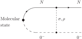
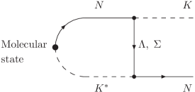
(a)	(b)	(c)

Figure 2: The diagrams for $\Theta^{+}$ decays. (a) and (b) correspond to the molecular states which are of $P$-$N$ or $V$-$N$ types. The pseudoscalar $K$($0^{-}$) should be replaced by $D$ or $B$ and $K^{*}$($1^{-}$) should be replaced by $D^{*}$ or $B^{*}$ for $\Theta_{c}$ and $\Theta_{b}$ respectively.

We will use harmonic oscillator modelharmonic to estimate the decay amplitude of a molecular state. The detail expressions are listed in Appendix B.

II.4 The Mass and Width for $\Theta_{b}$

The above results for mixed state can also be applied to the $\Theta_{b}$ state. As indicated above, $\Delta_{s}$ may be completely different from $\Delta_{c}$. For the same reason $g_{s}$ is expected to be different than $g_{c}$, but one can expect $\Delta_{c}$ and $g_{c}$ are related to $\Delta_{b}$ and $g_{b}$ since both $\Delta$ and $g$ are due to an exchange of a heavy anti-quark ($\bar{c}$ or $\bar{b}$) with a quark accompanied by a gluon exchange for the leading order. By the one-gluon-exchange (OGE) mechanism OGE , one may expect that the leading order of the effective potential is approximately proportional to the distance between the two constituents (here they refer to a light quark in the diqaurk and a heavy quark in the triquark) and thus inversely proportional to the reduced mass. We can roughly have

$$\frac{\Delta_{b}}{\Delta_{c}} = \frac{m_{\mu}(BN)}{m_{\mu}(DN)}=\frac{m_{B}(m_{D}+m_{N})}{m_{D}(m_{B}+m_{N})}=1.28,$$

$$\frac{\Delta_{b}}{\Delta_{c}} = \frac{m_{\mu}(B^{*}N)}{m_{\mu}(D^{*}N)}=\frac{m_{B^{*}}(m_{D^{*}}+m_{N})}{m_{D^{*}}(m_{B^{*}}+m_{N})}=1.17,$$ (13)

here $m_{\mu}(DN)$, $m_{\mu}(BN)$, $m_{\mu}(D^{*}N)$ and $m_{\mu}(B^{*}N)$ are respectively the reduced masses of $DN$, $BN$, $D^{*}N$ and $B^{*}N$ system. We use similar relation for $g_{b}/g_{c}$.

III Numerical Result

We are now ready to carry out numerical analysis. For the on-shell vertex parameters involved, we follow referencesLin ; Wujun ; Bracco ; Deandrea ; Casal ; 9901431 ; 0208168 to use:

$g_{NN\pi}=g_{NN\sigma}=13.5$, $g_{NN\rho}=3.25$ Lin .

$g_{KK\sigma}=4.50$ GeV; $g_{DD\sigma}=12.0$ GeV; $g_{BB\sigma}=35.0$ GeV Wujun .

$g_{KK\rho}=8.49$ Bracco ; Deandrea .

$g_{K^{*}K^{*}\pi}=g_{K^{*}K^{*}\sigma}=8.0$, $g_{D^{*}D^{*}\pi}=g_{D^{*}D^{*}\sigma}=3.5$, $g_{B^{*}B^{*}\pi}=g_{B^{*}B^{*}\sigma}=4.8$ Deandrea ; Casal ,

$g_{D^{*}D^{*}\rho}=g_{B^{*}B^{*}\rho}=2.9$ Bracco ; Deandrea ,

$g_{K^{*}K^{*}\rho}=4.8$. $g_{D^{*}D\pi}=18$, $g_{B^{*}B\pi}=49.1$ 9901431 .

$g_{DD\rho}=3.81$, $g_{BB\rho}=5.37$, $g_{D^{*}D\rho}=4.71$ GeV^-1, $g_{B^{*}B\rho}=5.70$ GeV^-1 0208168 .

It is generally believed that the parameter $\Lambda$ in the form factor is around 1 GeV, but the concrete number can vary in a certain range. If the value of $\Lambda$ is too small, the two constituents ($PN$ or $VN$) cannot be bound at all, i.e. the supposed molecular state does not exist, whereas, if the value of $\Lambda$ is too large, the binding energy becomes negative. We will allow $\Lambda$ to vary up to a few GeV. By solving the Schrödinger equation, we notice that for the $PN-$system ($KN,\;DN,\;BN$), the value of $\Lambda$ can be $1.5\sim 2.5$ GeV, and for the $VN-$system ($K^{*}N$, $D^{*}N$, $B^{*}N$) it is 0.5$\sim$1.5 GeV.

Solving the Schrödinger equation with the potential derived in the linear $\sigma$-model, we obtain the binding energies for pure molecular states of $KN$, $K^{*}N$, $DN$, $D^{*}N$, $BN$ and $B^{*}N$. The predicted values are listed in Table 1. The masses of the molecular states are given by $M_{Mole}=m_{N}+M_{P(V)}+E_{P(V)N}$ which are also listed in Table 1.

$P$-$N$ System			$V$-$N$ System
$\Lambda:1.5\sim 2.5$ GeV			$\Lambda:0.5\sim 1.5$ GeV
$E_{KN}$(MeV)	$E_{DN}$ (MeV)	$E_{BN}$ (MeV)	$E_{K^{*}N}$ (MeV)	$E_{D^{*}N}$ (MeV)	$E_{B^{*}N}$ (MeV)
$0\sim 25$	$0\sim 13$	$0\sim 9$	$0\sim 10$	$0\sim 4$	$0\sim 2$
$M_{KN}$(MeV)	$M_{DN}$ (MeV)	$M_{BN}$ (MeV)	$M_{K^{*}N}$ (MeV)	$M_{D^{*}N}$ (MeV)	$M_{B^{*}N}$ (MeV)
$1432\sim 1457$	$2803\sim 2816$	$6217\sim 6226$	$1830\sim 1840$	$2945\sim 2949$	$6263\sim 6265$

Table 1: The binding energies $E_{Mole}$ and $M_{Mole}$ for various systems.

III.1 The Mixing Parameters

Several groups have evaluated the masses of pure pentaquarks in different models. In our numerical evaluations, for concreteness we adopt the triquark-diquark structure proposed by Ref. Lipkin1 ; Lipkin2 .

a. The Results for $\Theta^{+}$

The value 1592 MeV for the mass of $\Theta^{+}$ obtained by Karliner and Lipkin is greater than the measured value (1540 MeV). To obtain a lower eigenmass, one must mix it with a state which also has a mass larger than the observed one. If a state with a lower mass is used, the resulting lower eigenstate would have a mass even lower in contradiction with data. This forbids $KN$ molecular state to be the one to mix with. The state which the pure pentaquark will mix with should be a molecular state of $K^{*}N$ type. One should identify $|\Psi_{-}\rangle$ as the $\Theta^{+}$ state. By fitting data, we have obtained the mixing parameter $\Delta_{s}$ and $x_{s}$ and other quantities. We have

$$x_{s}=0.46\sim 0.57,\;\;\;\;\Delta_{s}=101\sim 137\mbox{(MeV)},$$

$$\Gamma_{\Theta^{+}}=0.66\sim 1.26\mbox{(MeV)},\;\;\;\;\sin\theta=0.36\sim 0.41,$$

$$M_{+}=1879\sim 1889\mbox{(MeV)},\;\;\;\;\Gamma_{+}=103\sim 155\mbox{(MeV)}.$$ (14)

Here $M_{+}$ and $\Gamma_{+}$ are the mass and decay width of the partner state of $\Theta^{+}$ which corresponds to the larger eigenvalue.

One notes that a state of mass around 1885 MeV and broad width around 130 MeV is predicted. This state is above the $N$-$K$ and $N$-$K^{*}$ threshold and therefore may decay into them by strong interaction. One immediate question arises, why this state has not been discovered. There are several factors which may have contributed to the non-observation of this state if it exist, one of them is that a messy hadron spectra in that energy region where the expected resonance is hard to be clearly pinned down and mis-identified as background. Of course, at present, we cannot confirm the picture of mixing, namely it could be wrong and the resonance would be completely interpreted as a pure pentaquark.

b. The Results for $\Theta_{c}$ and $\Theta_{b}$

In the case of $\Theta_{c}$, both molecular masses of $N$-$D$ and $N$-$D^{*}$, and also the mass of the pure pentaquark are below the observed mass, a mixing of the pure pentaquark and molecular states can give correct mass. We also assume $\Theta_{b}$ to be in a similar situation.

(i) The case of $P$-$N$ molecular states

First we suppose that the molecular states of $DN$ and $BN$ mix with the pure pentaquarks $uudd\bar{c}$ and $uudd\bar{b}$ to construct $\Theta_{c}$ and $\Theta_{b}$. We have

$$\mbox{For the $\Theta_{c}$ State}: x_{c}=-0.69\sim-0.98,\;\;\;\;\Delta_{c}=127\sim 229\mbox{(MeV)},$$

$$\Gamma_{\Theta_{c}}=6.9\sim 12.5\mbox{(MeV)},\;\;\;\;\sin\theta=0.90\sim 0.80,$$

$$M_{-}=2631\sim 2748\mbox{(MeV)}.$$

$$\mbox{For the $\Theta_{b}$ State}: x_{b}=-0.69\sim-0.98,\;\;\;\;\Delta_{b}=162\sim 292\mbox{(MeV)},\;\;\;\;\sin\theta=0.89\sim 0.78$$ (15)

$$M_{\Theta_{b}}=6458\sim 6647\mbox{(MeV)},\;\;\;\;\Gamma_{\Theta_{b}}=2.6\sim 1.9\mbox{(MeV)}$$

$$M_{-}=5984\sim 6134\mbox{(MeV)}.$$

For the above two cases, the larger one of the two eigenvalues corresponds is the observed $\Theta_{c}$. $M_{-}$ is the mass of another eigenstate which is below the $N$-$D$ and $N$-$B$ threshold and therefore do not have strong decay channels. They can easily escape the detection. For the charged $\Theta_{b}$, there might be a trace of energy deposit on its path in a drift chamber and this signal may be used to identify its existence.

(ii) The case of $V$-$N$ molecular states

If the molecular states in $\Theta_{c}$ and $\Theta_{b}$ are $D^{*}N$ and $B^{*}N$, the results are different from the $P$-$N$ case. We have

$$\mbox{For the $\Theta_{c}$ State}: x_{c}=-0.81\sim-1.18,\;\;\;\;\Delta_{c}=90\sim 139\mbox{(MeV)},$$

$$\Gamma_{\Theta_{c}}=3.3\sim 15.3\mbox{(MeV)},\;\;\;\;\sin\theta=0.85\sim 0.76$$

$$M_{-}=2825\sim 2892\mbox{(MeV)},\;\;\;\Gamma_{-}=53.5\sim 109.9\mbox{(MeV)}.$$

$$\mbox{For the $\Theta_{b}$ State}: x_{b}=-0.81\sim-1.18,\;\;\;\;\Delta_{b}=112\sim 173\mbox{(MeV)},\;\;\;\;\sin\theta=0.91\sim 0.79,$$ (16)

$$M_{\Theta_{b}}=6426\sim 6552\mbox{(MeV)},\;\;\;\;\Gamma_{\Theta_{b}}=3.1\sim 12.7\mbox{(MeV)},$$

$$M_{-}=6128\sim 6211\mbox{(MeV)}.$$

Again the larger one of the two eigenvalues corresponds to the observed $\Theta_{c,b}$ and $M_{-}$ is the mass of another eigenstate. It is interesting to note that in this case the light partner of $\Theta_{b}$ is below the threshold of $N$-$B$ and therefore has no strong decay channel, but the light partner of $\Theta_{c}$ is above the $N$-$D$ threshold and can decay into $N+D$ by strong interaction via the diagram shown in Fig. 2(c). This state however has a broad width which may be difficult to identify. If future experiments with high precision still do not discover such a state, the mixing of $D^{*}$-$N$ molecular state with a pure pentaquark should be ruled out.

IV Multi-state mixing

As pointed out in the introduction, there could be multi-state mixing among pentaquark and molecular states of N-P and N-V types. For example the mechanisms shown in Fig.2 (b) and (c) can also mix the N-P and N-V states. By adjusting relevant parameters, the measured values can be easily re-produced. Allowing pentaquark, N-P and N-V states to mix, the effective Hamiltonian can be parameterized as

$$H=\left(\begin{array}[]{ccc}M_{Penta}&\Delta_{1}&\Delta_{2}\\ \Delta_{1}^{*}&M_{PN}&\epsilon\\ \Delta_{2}^{*}&\epsilon^{*}&M_{VN}\end{array}\right)\;,$$ (20)

where $\Delta_{1,2}$, and $\epsilon$ are the parameters describing the mixing among pentquark and molecular states. Now, the hamiltonian is expressed by a $3\times 3$ matrix instead of $2\times 2$ matrix discussed in last section.

In the cases discussed in the previous section the pure pentaquark and molecular states have masses significantly different from that of the observed states. This implies that the mixing needed to explain the data is large. The mixing depends on the size of the parameter $\Delta_{i}$ which is of order 100 MeV. The parameter $\epsilon$ which mixes the N-P and N-V states can be obtained in our approach by calculating diagrams Fig.2 (b) and (c). We find that the parameter $\epsilon$ is of order a few MeV which is considerably smaller than $\Delta_{i}$ needed to explain data. Neglecting the mixing between N-P and V-P in our analysis, i.e. setting $\epsilon$ to be zero, will not affect the main features of the results. We will take this simple case to illustrate how we can obtain the correct masses and correlations of the mixing parameters with the three-state mixing.

With the above hamiltonian, there are three eigenstates with one of them being identified as the observed physical states ($\Theta^{+},\;\Theta_{c}$ and possible $\Theta_{b}$). There may exist two other physical states. These states have not been discovered may be due to the same reasons discussed earlier for the other physical state in the case of two state mixing.

(a) For $\Theta^{+}$.

The observed state ($\Theta^{+}$) must be identified as the state with the middle eigenmass $M_{M}$ shown in Fig.3 (a). To fulfill this requirement, we must restrict the two mixing parameters $\Delta_{1}^{(s)}$ and $\Delta_{2}^{(s)}$ within a certain range. Fig.3 (b) demonstrates the relation between $\Delta_{1}^{(s)}$ and $\Delta_{2}^{(s)}$ and ranges for them. We use $M_{H}$ and $M_{L}$ to denote the masses corresponding to the heavier and the lighter physical states(see Fig. 3). The bands described in Fig. 3 (a) and (b) come from the experimental error of $M_{\Theta^{+}}$ and the theoretical uncertainties of the binding energies of $KN$ and $K^{*}N$ systems. One notes that the P-N state can also play significant role in the mixing.

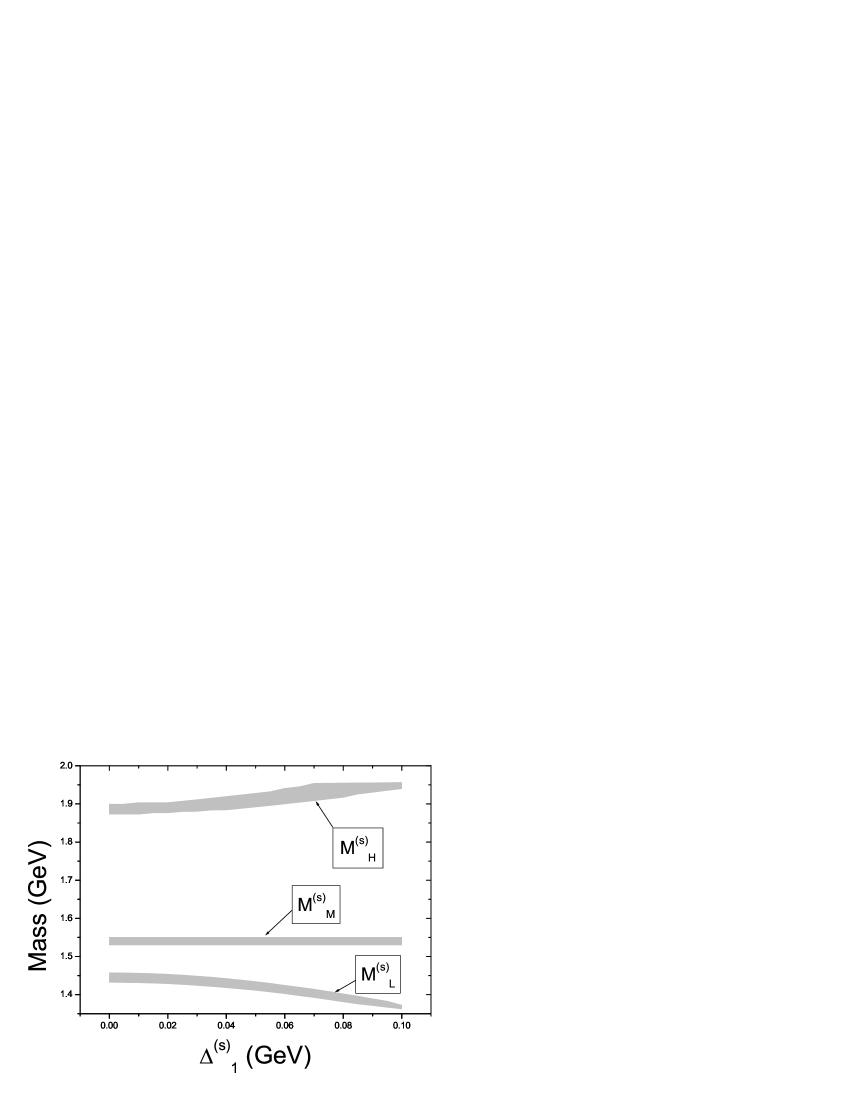
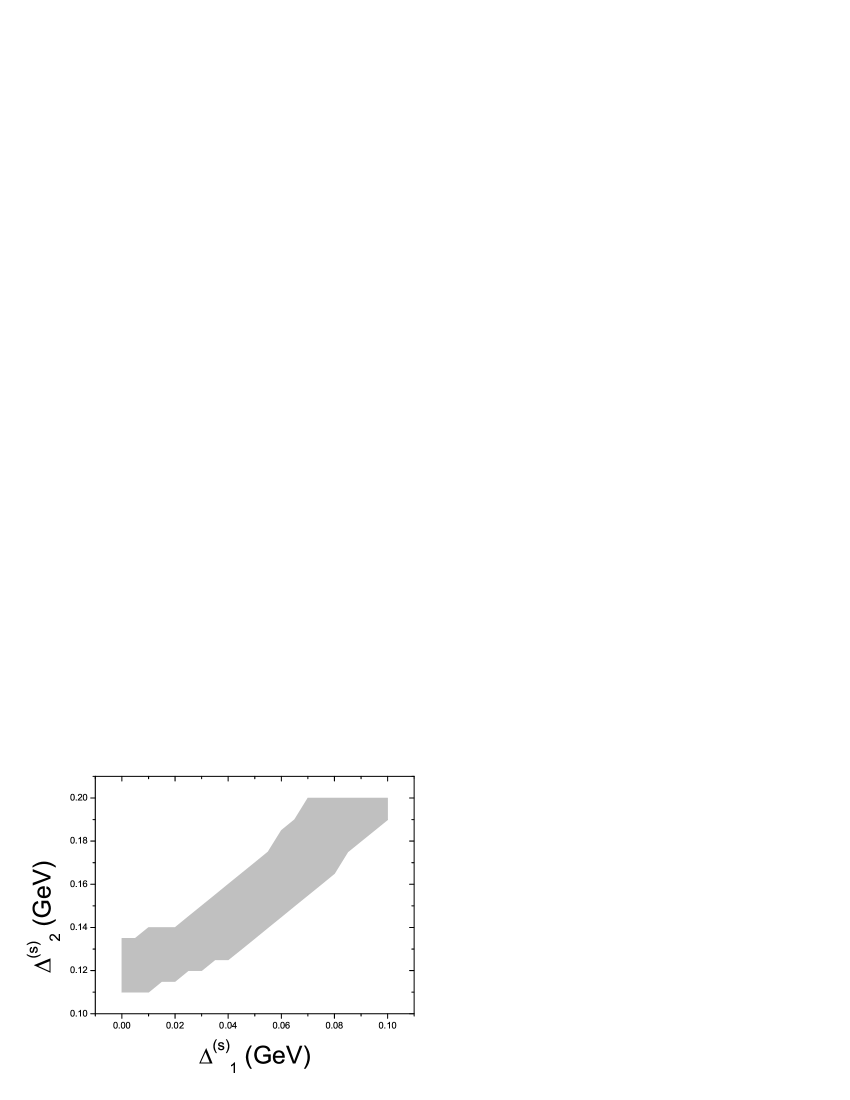
(a)	(b)

Figure 3: (a) and (b) describe the dependence of $M_{L}^{(s)}$, $M_{M}^{(s)}$ and $M_{H}^{(s)}$ on $\Delta_{1}^{(s)}$, and relation between $\Delta_{1}^{(s)}$ and $\Delta_{2}^{(s)}$, respectively. The state with middle eigenmass corresponds to the observed state $\Theta^{+}$.

(b) For $\Theta_{c}$.

Different from the case of $\Theta^{+}$, the largest one among the three physical states corresponds to the observed $\Theta_{c}$, when we diagonalize the three-states mixing hamiltonian (20). $M_{M}^{(c)}$ and $M_{L}^{(c)}$ are other two physical states having middle and lower eigenmasses respectively. Similarly, we also use two diagrams to demonstrate the relations between $M_{i}^{(c)}$ and $\Delta_{1}^{(c)}$, and $\Delta_{1}^{(c)}$ and $\Delta_{2}^{(c)}$ (see Fig. 4 (a) and (b)).

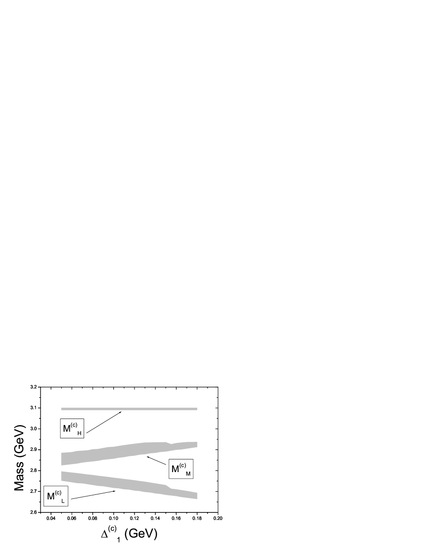
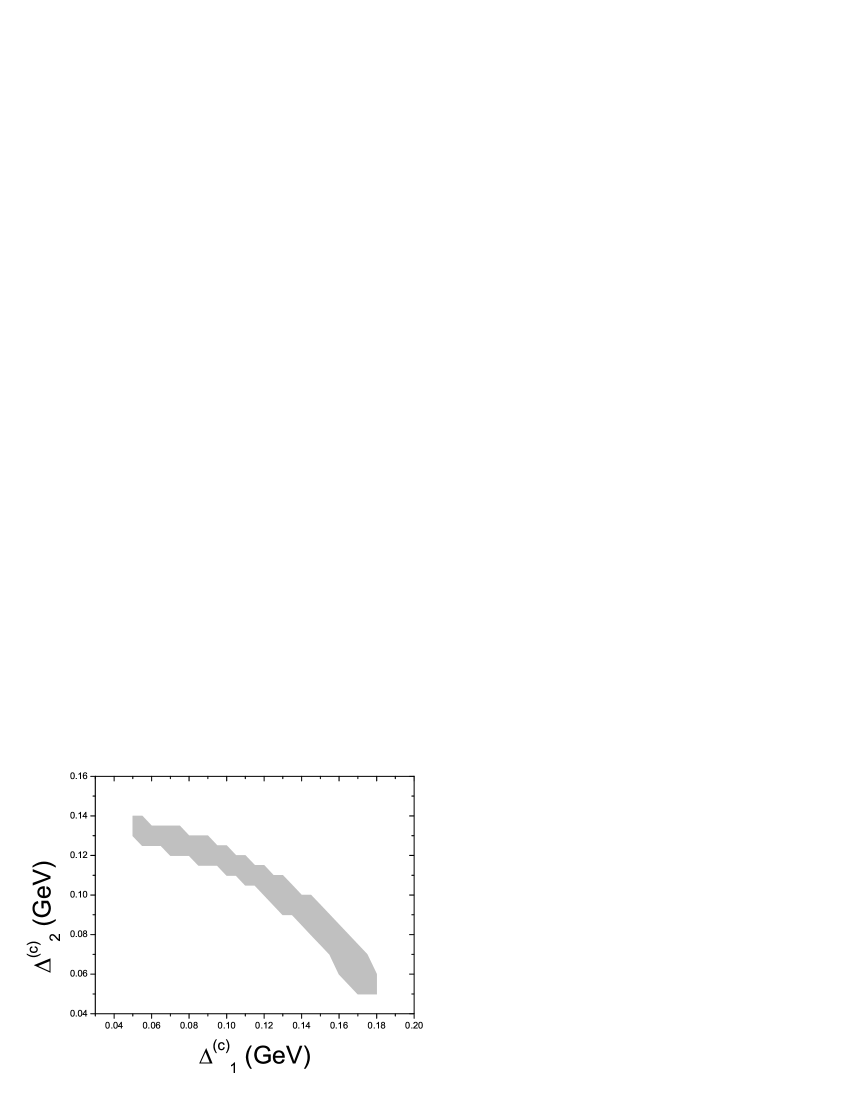
(a)	(b)

Figure 4: (a) and (b) describe the dependence of $M_{L}^{(c)}$, $M_{M}^{(c)}$ and $M_{H}^{(c)}$ on $\Delta_{1}^{(c)}$, and the relation between $\Delta_{1}^{(c)}$ and $\Delta_{2}^{(c)}$, respectively. The highest state corresponds to the observed $\Theta^{c}$.

(c) For $\Theta_{b}$.

In analog to the case of two-state mixing in last section, we apply the relations (13) of $\Delta_{1}^{(c)}$, $\Delta_{2}^{(c)}$ with $\Delta_{1}^{(b)}$, $\Delta_{2}^{(b)}$ to predict three physical states, whose masses are denoted as $M_{H}^{(b)}$, $M_{M}^{(b)}$ and $M_{L}^{(b)}$ respectively. We may expect that the state having the largest eigenmass $M_{H}^{(b)}$ corresponds to $\Theta_{b}$ which is a counterpart of the observed $\Theta_{c}$. In Fig. 5, we draw a diagram depicting the relations of the masses of the three physical states.

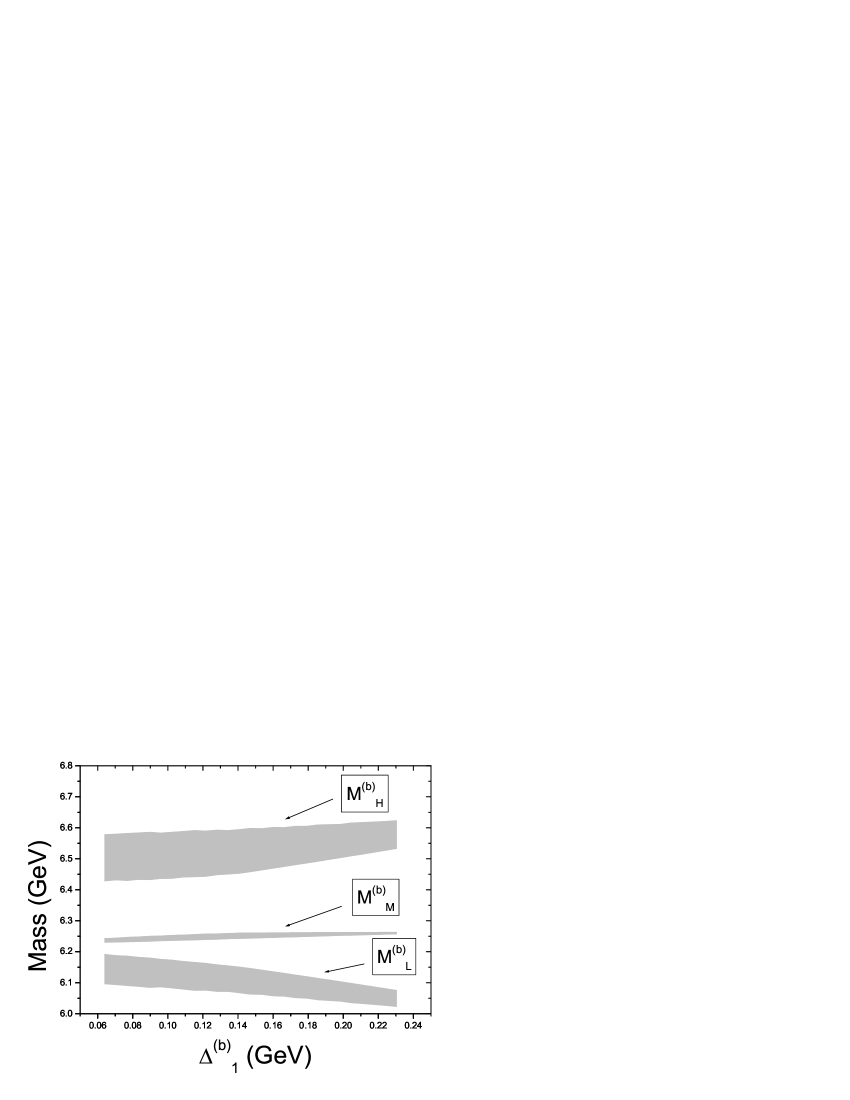
Figure 5: The dependence of $M_{L}^{(b)}$, $M_{M}^{(b)}$ and $M_{H}^{(b)}$ on $\Delta_{1}^{(b)}$

Whether there is significant three state mixing, that is both $\Delta_{1}$ and $\Delta_{2}$ are sizeable, has to be determined by future experimental data.

V Conclusion and discussion

In this work, motivated by the fact that the theoretically evaluated masses and widths of pure pentaquark or molecular states do not coincide with the observed $\Theta^{+}$ and $\Theta_{c}$ states, we have studied some consequences by assuming that the observed resonances $\Theta^{+}$ and $\Theta_{c}$ are mixtures of pure pentaquark and molecular states.

The pure pentaquarks may be in the triquark-diquark or diquark-diquark-antiquark structures, while the molecular states in fact are only a re-combination of the quark constituents and colors, i.e. another component in the Hilbert space. Therefore a mixing between the molecular state and pure pentaquark is possible. Combining theoretical estimates for the masses of the pure pentaquark given in the literatures and our estimate for the masses of pure molecular states in the linear $\sigma$-model, we estimated the mixing parameters, $\Delta_{i}$ (here i=s,c) by fitting data.

We find that through the mixing mechanism it is possible to obtain the observed masses for $\Theta^{+}$ and $\Theta_{c}$, and also possible to obtain narrow widths for these states through destructive interferences even if the pure pentaquark and the molecular states may have broader decay widths. The mixings are sizeable, but the dominant components of the observed states are pentaquark states.

An interesting prediction of mixing of pure pentaquark and molecular states is that there exists another physical state. In the case of $\Theta^{+}$, with the pure pentaquark mass predicted by the triquark-diquark modelLipkin1 , the state to be mixed is the $N$-$K^{*}$ molecular state. The resulting heavier physical state mass is predicted to be in the range $1879\sim 1889$ MeV with a width in the range $103\sim 155$ MeV. Since this state is above the producction threshold of $N$-$K$ and $N$-$K^{*}$, its strong decays into $N$-$K$ and $N$-$K^{*}$ can be used to discover such a state. At present there is no evidence for such a state. It may be due to experimental sensitivity since this is a region where there is a mess spectra, and this physical state has a broad width, so that it might be hidden in the forest of hadrons in the region and is mis-identified as the background. Of course there is also the possibility that the mixing for $\Theta^{+}$ is not needed and the pure pentaquark state has the right properties as attempted by many investigations.

For $\Theta_{c}$, it is another story, by contraries. If the pure pentaquark mixes with a $N$-$D$ molecular state, the mixing mechanism would predict that the mass of the other state is below the threshold of $N$-$D$. This state is stable against strong interaction, and may have escaped detection in the detector. There may be several weak decay channels, but difficult to detect either. Whereas if the pure pentaquark mixes with a $N$-$D^{*}$ state the light partner of $\Theta_{c}$ is above the $N$-$D$ threshold and can decay into $N+D$ by strong interaction. This state however has a broad width which may be difficult to identify. If future experiments with high precision still do not discover such a state, the mixing of $D^{*}$-$N$ molecular state with a pure pentaquark should be ruled out.

For $\Theta_{b}$ the light partner state is below the $N$-$B$ threshold for both the cases that the pure pentaquark mixes with a $B$-$N$ or $B^{*}$-$N$ molecular state. Since the light partner state is charged, although it does not have strong decay modes, it may leave trace by depositing energy in the medium when passing through a detector, such as a drift chamber. We encourage our experimental colleagues to carry out a search in the relevant region.

Obviously there could be multi-state mixing among diqaurk-diqaurk-antiqaurk, diqaurk-triquark and molecular state(s). By adjusting parameters (there are more of them than in the two-state mixing), the measured values can be re-produced. In section IV, we illustrate possible changes if three-state mixing is considered. We find that for the present experimental data, it is easy to restore the case for two-state mixing by requiring one of $\Delta_{i}$ to be zero. Thus the main feature is clearly given in the two-state mixing case. Since we cannot reliably evaluate the mixing parameter from any solid theoretical ground, considering mixing among more states does not provide us with further information. At present, the two-state mixing can result in values which well explain the spectra and narrow widths of $\Theta^{+}$, $\Theta_{c}$ and predict possible $\Theta_{b}$. However, in the future more accurate measurements on properties of the resonances may demand such multi-state mixing.

As a conclusion, a mixing between a pure pentaquark and a molecular state may be reasonable and by this picture, we can explain the mass spectra and widths of the observed $\Theta^{+}$ and $\Theta_{c}$ even the theoretical estimations based on the pure pentaquark given in the literatures obviously deviate from data. Applying the same mechanism, we have predicted the mass and width of $\Theta_{b}$ which can be tested in the future experiments. Moreover, multi-state mixing may be required when more accurate measurements are made in the future.

Acknowledgment:

We would like to thank professors Lipkin, Toki, K.T. Chao, B.Q. Ma, B.S. Zou for many useful discussions. This work is partly supported by the National Natural Science Foundation of China.

Appendix A

(i) The effective potential for the nucleon and pseudoscalar meson system.

(1) $\sigma$ exchange.

$$V^{\mathbf{P}-N}_{\sigma}(\mathbf{q}) = \frac{-g_{NN\sigma}\,g_{PP\sigma}}{2m_{a}(\mathbf{q}^{2}+{{m_{\sigma}}}^{2})}\bigg{[}1-\frac{{{\mathbf{p}}}_{1}^{2}}{2\,{m_{a}}^{2}}-\frac{\mathbf{q}^{2}}{8m_{N}^{2}}-\frac{\mathbf{q}\cdot\mathbf{p}_{1}+3\mathbf{p}_{1}\cdot\mathbf{q}}{8m_{N}^{2}}-\frac{\mathbf{p}_{1}^{2}}{2m_{N}^{2}}$$ (21)

$$-\frac{i}{4m_{N}^{2}}{\mbox{\boldmath$\sigma$}_{2}}\cdot\left(\mathbf{q}\times\mathbf{p}_{1}\right)\bigg{]}\bigg{(}\frac{{{\Lambda}^{2}-{{m_{\sigma}}}^{2}}}{{\mathbf{q}^{2}+{\Lambda}^{2}}}\bigg{)}^{2},$$

taking the Fourier transformation, we obtain

$$V^{\mathbf{P}-N}_{\sigma}(r) = \frac{-g_{NN\sigma}\,g_{PP\sigma}}{2m_{a}}\bigg{\{}f_{\sigma}(r)-\frac{9}{8m_{N}^{2}}F_{\sigma}(r)-\bigg{(}\frac{1}{2\,{m_{a}}^{2}}+\frac{1}{2m_{N}^{2}}\bigg{)}{{\mathbf{p}}}_{1}^{2}f_{\sigma}(r)$$ (22)

$$+\frac{[\mathbf{\nabla}^{2}f_{\sigma}(r)]}{8m_{N}^{2}}+\frac{i\mathbf{p}_{1}\cdot\mathbf{r}}{2m_{N}^{2}}F_{\sigma}(r)-\frac{\mathbf{S}_{2}\cdot\mathbf{L}}{2m_{N}^{2}}F_{\sigma}(r)\bigg{\}}.$$

where

$$f_{\sigma}(r) = \frac{\displaystyle e^{-m_{\sigma}r}}{\displaystyle 4\pi r}-\frac{\displaystyle e^{-\Lambda r}}{\displaystyle 4\pi r}+\frac{\displaystyle(m_{\sigma}^{2}-\Lambda^{2})e^{-\Lambda r}}{\displaystyle 8\pi\Lambda},$$

$$F_{\sigma}(r) = \frac{1}{\displaystyle r}\frac{\displaystyle\partial}{\displaystyle\partial r}f_{\sigma}(r).$$

(2) $\rho$ exchange.

$$V^{\mathbf{P}-N}_{\rho}(\mathbf{q}) = \frac{g_{NN\rho}\,g_{PP\rho}}{\mathbf{q}^{2}+{{m_{\rho}}}^{2}}\bigg{\{}1-\frac{\mathbf{q}^{2}}{8m_{N}^{2}}-\frac{\mathbf{q}\cdot\mathbf{p}_{1}-\mathbf{p}_{1}\cdot\mathbf{q}}{8m_{N}^{2}}+\frac{i{\mbox{\boldmath$\sigma$}_{2}}\cdot(\mathbf{q}\times\mathbf{p}_{1})}{4m_{N}^{2}}+\frac{1}{4m_{N}m_{a}}[\mathbf{q}^{2}+4\mathbf{p}_{1}^{2}$$ (23)

$$+2\mathbf{q}\cdot\mathbf{p}_{1}+2\mathbf{p}_{1}\cdot\mathbf{q}+2i{\mbox{\boldmath$\sigma$}_{2}}\cdot(\mathbf{q}\times\mathbf{p}_{1})]\bigg{\}}\bigg{(}\frac{\displaystyle\Lambda^{2}-m_{\rho}^{2}}{\displaystyle\Lambda^{2}+\mathbf{q}^{2}}\bigg{)}^{2}$$

taking the Fourier transformation, we get

$$V^{\mathbf{P}-N}_{\rho}(r) = g_{NN\rho}\,g_{PP\rho}\bigg{\{}f_{\rho}(r)-\frac{3}{8m_{N}^{2}}F_{\rho}(r)+\frac{[\mathbf{\nabla}^{2}f_{\rho}(r)]}{8m_{N}^{2}}+\frac{\mathbf{S}_{2}\cdot\mathbf{L}}{2m_{N}^{2}}F_{\rho}(r)-\frac{[\mathbf{\nabla}^{2}f_{\rho}(r)]}{4m_{N}m_{a}}$$ (24)

$$+\frac{1}{4m_{N}m_{a}}\left[4\mathbf{p}_{1}^{2}f_{\rho}(r)+6F_{\rho}(r)-4i\mathbf{p}_{1}\cdot\mathbf{r}F_{\rho}(r)+4\mathbf{S}_{2}\cdot\mathbf{L}F_{\rho}(r)\right]\bigg{\}},$$

where

$$f_{\rho}(r) = \frac{\displaystyle e^{-m_{\rho}r}}{\displaystyle 4\pi r}-\frac{\displaystyle e^{-\Lambda r}}{\displaystyle 4\pi r}+\frac{\displaystyle(m_{\rho}^{2}-\Lambda^{2})e^{-\Lambda r}}{\displaystyle 8\pi\Lambda},$$

$$F_{\rho}(r) = \frac{1}{\displaystyle r}\frac{\displaystyle\partial}{\displaystyle\partial r}f_{\rho}(r).$$

(ii) The effective potential for the nucleon and vector meson system.

(1) pion exchang.

$$V^{\mathbf{V}-N}_{\pi}(\mathbf{q}) = -\frac{g_{NN\pi}\,g_{VV\pi}}{4m_{N}(\mathbf{q}^{2}+m_{\pi}^{2})}(\mathbf{S}_{1}\cdot\mathbf{q})(\mathbf{S}_{2}\cdot\mathbf{q})\bigg{(}\frac{\displaystyle\Lambda^{2}-m_{\pi}^{2}}{\displaystyle\Lambda^{2}+\mathbf{q}^{2}}\bigg{)}^{2},$$ (25)

taking a Fourier transformation, we get

$$V^{\mathbf{V}-N}_{\pi}(r) = \frac{g_{NN\pi}\,g_{VV\pi}}{4m_{N}}(\mathbf{S}_{1}\cdot\mathbf{\nabla})(\mathbf{S}_{2}\cdot\mathbf{\nabla})f_{\pi}(r),$$ (26)

here

$$f_{\pi}(r) = \frac{\displaystyle e^{-m_{\pi}r}}{\displaystyle 4\pi r}-\frac{\displaystyle e^{-\Lambda r}}{\displaystyle 4\pi r}+\frac{\displaystyle({m_{\pi}}^{2}-\Lambda^{2})e^{-\Lambda r}}{\displaystyle 8\pi\Lambda}.$$

(2) $\sigma$ exchange.

$$V^{\mathbf{V}-N}_{\sigma}(\mathbf{q}) = -\frac{g_{NN\sigma}\,g_{VV\sigma}\,m_{b}}{2(\mathbf{q}^{2}+{{m_{\sigma}}}^{2})}\bigg{[}-1+\frac{{{\mathbf{p}}}_{1}^{2}}{6\,{m_{b}}^{2}}+\frac{2\mathbf{p}_{1}\cdot\mathbf{q}}{3m_{b}^{2}}-\frac{i\mathbf{S}_{1}\cdot(\mathbf{q}\times\mathbf{p}_{1})}{4m_{b}^{2}}$$ (27)

$$+\frac{\mathbf{p}_{1}\cdot\mathbf{q}-\mathbf{q}\cdot\mathbf{p}_{1}}{8m_{N}^{2}}+\frac{\mathbf{q}^{2}}{8m_{N}^{2}}-\frac{i\mathbf{S}_{2}\cdot(\mathbf{q}\times\mathbf{p}_{1})}{4m_{N}^{2}}\bigg{]}\bigg{(}\frac{{{\Lambda}^{2}-{{m_{\sigma}}}^{2}}}{{\mathbf{q}^{2}+{\Lambda}^{2}}}\bigg{)}^{2},$$

taking a Fourier transformation, we obtain

$$V^{\mathbf{V}-N}_{\sigma}(r) = -\frac{g_{NN\sigma}\,g_{VV\sigma}\,m_{b}}{2}\bigg{\{}-f_{\sigma}(r)-\frac{3}{8m_{N}^{2}}F_{\sigma}(r)+\frac{{{\mathbf{p}}}^{2}}{6{m_{b}}^{2}}f_{\sigma}(r)-\frac{\mathbf{S}_{1}\cdot\mathbf{L}}{4m_{b}^{2}}F_{\sigma}(r)$$ (28)

$$-\frac{2i\mathbf{p}_{1}\cdot\mathbf{r}}{3m_{b}^{2}}F_{\sigma}(r)-\frac{[\mathbf{\nabla}^{2}f_{\sigma}(r)]}{8m_{N}^{2}}-\frac{\mathbf{S}_{2}\cdot\mathbf{L}}{2m_{N}^{2}}F_{\sigma}(r)\bigg{\}},$$

where

$$f_{\sigma}(r) = \frac{\displaystyle e^{-m_{\sigma}r}}{\displaystyle 4\pi r}-\frac{\displaystyle e^{-\Lambda r}}{\displaystyle 4\pi r}+\frac{\displaystyle(m_{\sigma}^{2}-\Lambda^{2})e^{-\Lambda r}}{\displaystyle 8\pi\Lambda},$$

$$F_{\sigma}(r) = \frac{1}{\displaystyle r}\frac{\displaystyle\partial}{\displaystyle\partial r}f_{\sigma}(r).$$

(3) $\rho$ exchange.

$$V^{\mathbf{V}-N}_{\rho}(\mathbf{q}) = \frac{g_{NN\rho}\,g_{VV\rho}}{\mathbf{q}^{2}+{{m_{\rho}}}^{2}}\bigg{[}1-\frac{\mathbf{q}^{2}}{8m_{N}^{2}}-\frac{\mathbf{p}_{1}\cdot\mathbf{q}-\mathbf{q}\cdot\mathbf{p}_{1}}{8m_{N}^{2}}+\frac{i\mathbf{S}_{2}\cdot(\mathbf{q}\times\mathbf{p}_{1})}{4m_{N}^{2}}+\frac{\mathbf{q}^{2}}{4m_{N}m_{1^{-}}}+\frac{\mathbf{p}_{1}^{2}}{6m_{N}m_{b}}$$ (29)

$$+\frac{\mathbf{p}_{1}\cdot\mathbf{q}}{2m_{N}m_{b}}+\frac{\mathbf{q}\cdot\mathbf{p}_{1}}{12m_{N}m_{b}}-\frac{i\mathbf{S}_{2}\cdot(\mathbf{q}\times\mathbf{p}_{1})}{6m_{N}m_{b}}-\frac{i\mathbf{S}_{1}\cdot(\mathbf{q}\times\mathbf{p}_{1})}{8m_{N}m_{b}}\bigg{]}\bigg{(}\frac{\displaystyle\Lambda^{2}-m_{\rho}^{2}}{\displaystyle\Lambda^{2}+\mathbf{q}^{2}}\bigg{)}^{2},$$

taking a Fourier transformation, we get

$$V^{\mathbf{V}-N}_{\rho}(r) = g_{NN\rho}\,g_{VV\rho}\bigg{\{}f_{\rho}(r)+\frac{3}{8m_{N}^{2}}F_{\rho}(r)-\frac{1}{2m_{N}m_{b}}F_{\rho}(r)+\frac{[\mathbf{\nabla}^{2}f_{\rho}(r)]}{8m_{N}^{2}}+\frac{\mathbf{S}_{2}\cdot\mathbf{L}}{4m_{N}^{2}}F_{\rho}(r)$$ (30)

$$-\frac{[\mathbf{\nabla}^{2}f_{\rho}(r)]}{4m_{N}m_{b}}+\frac{\mathbf{p}_{1}^{2}}{6m_{N}m_{b}}f_{\rho}(r)-\frac{7i\mathbf{r}\cdot\mathbf{p}_{1}}{12m_{N}m_{b}}F_{\rho}(r)-\frac{\mathbf{S}_{2}\cdot\mathbf{L}}{6m_{N}m_{b}}F_{\rho}(r)$$

$$-\frac{\mathbf{S}_{1}\cdot\mathbf{L}}{8m_{N}m_{b}}F_{\rho}(r)\bigg{\}},$$

here

$$f_{\rho}(r) = \frac{\displaystyle e^{-m_{\rho}r}}{\displaystyle 4\pi r}-\frac{\displaystyle e^{-\Lambda r}}{\displaystyle 4\pi r}+\frac{\displaystyle(m_{\rho}^{2}-\Lambda^{2})e^{-\Lambda r}}{\displaystyle 8\pi\Lambda},$$

$$F_{\rho}(r) = \frac{1}{\displaystyle r}\frac{\displaystyle\partial}{\displaystyle\partial r}f_{\rho}(r).$$

Appendix B
The molecular state is expressed asharmonic

$$|\phi_{Mole}(\mathbf{P},s)\rangle=A\cdot\sum_{spin}C^{s}_{s_{1},s_{2}}\chi_{s_{1},s_{2}}\int d\mathbf{p}_{1}d\mathbf{p}_{2}\psi(\mathbf{p}_{1},\mathbf{p}_{2})\delta^{3}(\mathbf{p}_{1}+\mathbf{p}_{2})b^{{\dagger}}_{p_{1},s_{1}}a^{{\dagger}}_{p_{2},s_{2}}|0\rangle,$$ (31)

where $C^{s}_{s_{1},s_{2}}$ is the C-G coefficients, $\chi_{s_{1},s_{2}}$ are the spin-wavefunctions and $A$ is a normalization constant. We normalize this fermion state as

$$\langle\phi_{Mole}(\mathbf{P}^{\prime})|\phi_{Mole}(\mathbf{P})\rangle=(2\pi)^{3}\frac{E_{P}}{M_{A}}\;\delta^{3}(\mathbf{P}^{\prime}-\mathbf{P}).$$ (32)

In Fig.2(a), we present the diagram for decay of the molecular state which is composed of a pseudoscalar meson and a nucleon in P-state, this transition occurs via exchanging $\sigma$ or $\rho$, the amplitudes are

$$\mathcal{M}(\sigma)^{(PN)} = A\cdot g_{NN\sigma}g_{PP\sigma}\int d\mathbf{p}_{1}d\mathbf{p}_{2}\sum_{spin}C^{s}_{s_{1},s_{2}}\chi_{s_{1},s_{2}}\bar{u}(P_{B},s_{B})u(p_{1},s_{1})\psi(\mathbf{p}_{1},\mathbf{p}_{2})$$ (33)

$$\times\delta^{3}(\mathbf{p}_{1}+\mathbf{p}_{2})\cdot\frac{1}{q^{2}-m_{\sigma}^{2}}\bigg{(}\frac{\displaystyle\Lambda^{2}-m_{\sigma}^{2}}{\displaystyle\Lambda^{2}-q^{2}}\bigg{)}^{2},$$

$$\mathcal{M}(\rho)^{(PN)} = A\cdot g_{NN\rho}g_{PP\rho}\int d\mathbf{p}_{1}d\mathbf{p}_{2}\sum_{spin}C^{s}_{s_{1},s_{2}}\chi_{s_{1},s_{2}}\bar{u}(P_{B},s_{B})\gamma^{\mu}u(p_{1},s_{1})(P_{C}+p_{2})^{\nu}$$ (34)

$$\times\psi(\mathbf{p}_{1},\mathbf{p}_{2})\delta^{3}(\mathbf{p}_{1}+\mathbf{p}_{2})\cdot\frac{g_{\mu\nu}}{q^{2}-m_{\rho}^{2}}\bigg{(}\frac{\displaystyle\Lambda^{2}-m_{\rho}^{2}}{\displaystyle\Lambda^{2}-q^{2}}\bigg{)}^{2}.$$

and the total amplitude is the sum of $\mathcal{M}^{(PN)}(\sigma)$ and $\mathcal{M}^{(PN)}(\rho)$.

In Fig.2(b), the molecular state consists of a vector meson and a nucleon, the corresponding amplitudes are

$$\mathcal{M}(\pi)^{(VN)} = A\cdot g_{NN\pi}g_{VP\pi}\int d\mathbf{p}_{1}d\mathbf{p}_{2}\sum_{spin}C^{s}_{s_{1},s_{2}}\chi_{s_{1},s_{2}}\bar{u}(P_{B},s_{B})\gamma^{5}u(p_{1},s_{1})(2P_{C}-p_{2})^{\mu}$$ (35)

$$\times\epsilon_{\mu}\psi(\mathbf{p}_{1},\mathbf{p}_{2})\delta^{3}(\mathbf{p}_{1}+\mathbf{p}_{2})\cdot\frac{1}{q^{2}-m_{\pi}^{2}}\bigg{(}\frac{\displaystyle\Lambda^{2}-m_{\pi}^{2}}{\displaystyle\Lambda^{2}-q^{2}}\bigg{)}^{2},$$

$$\mathcal{M}(\rho)^{(VN)} = A\cdot g_{NN\rho}g_{VP\rho}\int d\mathbf{p}_{1}d\mathbf{p}_{2}\sum_{spin}C^{s}_{s_{1},s_{2}}\chi_{s_{1},s_{2}}\bar{u}(P_{B},s_{B})\gamma^{\lambda}u(p_{1},s_{1})\varepsilon^{\alpha\beta\mu\nu}q_{\alpha}p_{2\mu}$$ (36)

$$\times\epsilon_{\nu}\psi(\mathbf{p}_{1},\mathbf{p}_{2})\delta^{3}(\mathbf{p}_{1}+\mathbf{p}_{2})\cdot\frac{g_{\lambda\beta}}{q^{2}-m_{\rho}^{2}}\bigg{(}\frac{\displaystyle\Lambda^{2}-m_{\rho}^{2}}{\displaystyle\Lambda^{2}-q^{2}}\bigg{)}^{2}.$$

and the total amplitude is the sum of $\mathcal{M}(\pi)^{(VN)}$ and $\mathcal{M}(\rho)^{(VN)}$.

References

- (1) LEPS collaboration, T. Nakano et al., Phys. Rev. Lett. 91, 012002 (2003), arXiv: hep-ex/0301020.
- (2) DIANA Collaboration, V.V. Barmin et al., Atom. Nucl. 66, 1715 (2003), arXiv: hep-ex/0304040.
- (3) CLAS Collaboration, S. Stepanyan et al., Phys. Rev. Lett. 91 252001 (2003), arXiv: hep-ex/0307018.
- (4) CLAS Collaboration, V. Kubarovsky et al., Phys. Rev. Lett. 92 032001 (2004), arXiv: hep-ex/0311046.
- (5) SAPHIR Collaboration, J. Barth et al., Phys. Lett. B 572 127 (2003), arXiv: hep-ex/0307083.
- (6) A.E. Asratyan, A.G. Dolgolenko and M.A. Kubantsev, arXiv: hep-ex/0309042.
- (7) HERMES Collaboration, A. Airapetian et al., Phys. Lett. B 585, 213 (2004), arXiv: hep-ex/0312044.
- (8) SVD Collaboration, A. Aleev et al., arXiv: hep-ex/0401024.
- (9) ZEUS Collaboration, S.V. Chekanov, arXiv: hep-ex/0403051.
- (10) COSY-TOF Collatoration, M. Abdel-Bary et al., arXiv: hep-ex/0403051.
- (11) R. Togoo et al., Proc. Mongolian Acad. Sci., 4 (2003) 2.
- (12) P. Z. Aslanyan, V. N. Emelyanenko and G. G. Rikhkvitzkaya, arXiv: hep-ex/0403044.
- (13) T. Nakano, talk at NSTAR 2004, March 24-27, Grenoble, France, arXiv: http://lpsc.in2p3.fr/congres/nstar2004/talks/nakano.pdf.
- (14) Y. A. Troyan et al., arXiv: hep-ex/0404003.
- (15) A.V. Manohar, Nucl. Phys. B 248, 19(1984); M. Chemtob, Nucl. Phys. B 256, 600(1985); M. Praszalowicz, in Skrmions and Anomalies, M. Jezabeck and M. Praszalowicz, eds. World Scientific, 112(1987); Phys. Lett. B 575, 234(2003), arXiv:hep-ph/0308114; Y. Oh, Phys. Lett. B 331, 362(1994); M.-L. Yan and X.-H. Meng, Commun. Theor. Phys. 24, 435(1995). D. Diakonov, V. Petrov and M.V. Polyakov, Z. Phys A 359 305 (1997).
- (16) H1 Collaboration, arXiv: hep-ex/0403017.
- (17) H. J. Lipkin, Phys. Lett. B , 484 (1987).
- (18) J.Z. Bai et al., (BES), Phys. Rev. D , 012004 (2004), arXiv: hep-ex/0402012. K. Abe et al., (Belle), arXiv: hep-ex/0409010. B. Aubert et al., (BaBar), arXiv: hep-ex/0408064. K.T. Knöpffe et al., (HERA-B), J. Phys. G , S1363-S1366 (2004), arXiv: hep-ex/0403020. D.O. Litvintsev, (CDF), arXiv: hep-ex/0410024. C. Pinkerton et al., (PHENIX), J. Phys. G 30:S1201 (2004); arXiv: nucl-ex/0404001. B. Aubert et al., (BABAR), arXiv: hep-ex/0502004.
- (19) Haiyan Gao, Bo-Qiang Ma, Mod. Phys. Lett. A 14, 2313-2319, 1999, arXiv: hep-ph/0305294. Fl. Stancu, D. O. Riska, Phys. Lett. B 575, 242-248, 2003, arXiv: hep-ph/0307010. Atsushi Hosaka, Phys. Lett. B 571, 55-60, 2003, arXiv: hep-ph/0307232. Shi-Lin Zhu, Phys. Rev. Lett. 91, 232002, 2003, arXiv: hep-ph/0307345. Xun Chen, Yajun Mao, Bo-Qiang Ma, Mod. Phys. Lett. A 19, 2289-2298, 2004, arXiv: hep-ph/0307381. Carl E. Carlson, Christopher D. Carone, Herry J. Kwee, Vahagn Nazaryan, Phys. Lett. B 573, 101-108, 2003, arXiv: hep-ph/0307396. Lie-Wen Chen, V. Greco, C. M. Ko, S. H. Lee, W. Liu, Phys. Lett. B 601, 34-40, 2004, arXiv: nucl-th/0308006. P.Bicudo, G. M. Marques, Phys. Rev. D 69, 011503, 2004, arXiv: hep-ph/0308073. Michal Praszalowicz, Phys. Lett. B 575, 234-241, 2003, arXiv: hep-ph/0308114. L. Ya. Glozman, Phys.Lett. B 575, 18-24, 2003, arXiv: hep-ph/0308232. R.D. Matheus, F.S. Navarra, M. Nielsen, R. Rodrigues da Silva, S.H. Lee, Phys. Lett. B 578, 323-329, 2004, arXiv: hep-ph/0309001. Yongseok Oh, Hungchong Kim, Su Houng Lee, Phys. Rev. D 69, 014009, 2004, arXiv: hep-ph/0310019. F.Huang, Z.Y.Zhang, Y.W.Yu, B.S.Zou, Phys. Lett. B 586, 69-74, 2004, arXiv: hep-ph/0310040. Yongseok Oh, Hungchong Kim, Su Houng Lee, Phys. Rev. D 69, 094009, 2004, arXiv: hep-ph/0310117. I.M.Narodetskii, Yu.A.Simonov, M.A.Trusov, A.I.Veselov, Phys. Lett. B 578, 318-322, 2004, arXiv: hep-ph/0310118. J. Letessier, G. Torrieri, S. Steinke, J. Rafelski, Phys. Rev. C 68, 061901, 2003, arXiv: hep-ph/0310188. Philip R. Page, arXiv: hep-ph/0310200. R. Bijker, M.M. Giannini, E. Santopinto, Eur. Phys. J. A 22, 319-329, 2004, arXiv: hep-ph/0310281. Qiang Zhao, Phys. Rev. D 69, 053009, 2004, arXiv: hep-ph/0310350. Peng-Zhi Huang, Wei-Zhen Deng, Xiao-Lin Chen, Shi-Lin Zhu, Phys. Rev. D 69, 074004, 2004, arXiv: hep-ph/0311108. K. Nakayama, K. Tsushima, Phys. Lett. B 583, 269-277, 2004, arXiv: hep-ph/0311112. A.R. Dzierba, D. Krop, M. Swat, A.P. Szczepaniak, S.Teige, Phys. Rev. D 69, 051901, 2004, arXiv: hep-ph/0311125. Y.-R. Liu, P.-Z. Huang, W.-Z. Deng, X.-L. Chen, Shi-Lin Zhu, Phys. Rev. C 69, 035205, 2004, arXiv: hep-ph/0312074. A.W. Thomas, K. Hicks, A. Hosaka, Prog. Theor. Phys. 111, 291-293, 2004, arXiv: hep-ph/0312083. M. Diehl, B. Pire, L. Szymanowski, Phys. Lett. B 584, 58-70, 2004, arXiv: hep-ph/0312125. P. Ko et al., arXiv: hep-ph/0312147. Bin Wu, Bo-Qiang Ma, Phys. Lett. B 586, 62-68, 2004, arXiv: hep-ph/0312326. W.-W. Li, Y.-R. Liu, P.-Z. Huang, W.-Z. Deng, X.-L. Chen, Shi-Lin Zhu, High Energy Phys. Nucl. Phys. 28, 918, 2004, arXiv: hep-ph/0312362. R. Bijker, M.M. Giannini, E. Santopinto, Rev. Mex. Fis. 50 S2, 88-95, 2004, arXiv: hep-ph/0312380. P. Bicudo, G. M. Marques, AIP Conf.Proc. 717 (2004) 467-474, arXiv: hep-ph/0312391. M. Bleicher, F.M. Liu, J. Aichelin, T. Pierog, K. Werner, Phys. Lett. B 595, 288-292, 2004, arXiv: hep-ph/0401049. Thomas Mehen, Carlos Schat, Phys. Lett. B 588, 67-73, 2004, arXiv: hep-ph/0401107. Michail P. Rekalo, Egle Tomasi-Gustafsson, Phys. Lett. B 591, 225-228, 2004, arXiv: hep-ph/0401162. Yu-xin Liu, Jing-sheng Li, Cheng-guang Bao, arXiv: hep-ph/0401197. Marek Karliner, Harry. J. Lipkin, Phys. Lett. B 594, 273-276, 2004, arXiv: hep-ph/0402008. Elizabeth Jenkins, Aneesh V. Manohar, JHEP 0406 (2004) 039, arXiv: hep-ph/0402024. Fl. Stancu, Phys. Lett. B 595, 269-276, 2004, arXiv: hep-ph/0402044. Thomas D. Cohen, Phys. Rev. D 70, 074023, 2004, arXiv: hep-ph/0402056. Gerald A. Miller, Phys. Rev. C 70, 022202, 2004, arXiv: nucl-th/0402099. Yu. N. Uzikov, arXiv: hep-ph/0402216. Seung-Il Nam, Atsushi Hosaka, Hyun-Chul Kim, arXiv: hep-ph/0403009. Xing-Chang Song, Shi-Lin Zhu, Mod. Phys. Lett. A 19, 2791-2797, 2004, arXiv: hep-ph/0403093. Frank E. Close, Qiang Zhao, Phys. Lett. B 590, 176-184, 2004, arXiv: hep-ph/0403159. N.I. Kochelev, H.-J. Lee, V. Vento, Phys. Lett. B594, 87-96, 2004, arXiv: hep-ph/0404065. Qiang Zhao, Frank E. Close, J. Phys. G 31, L1, 2005, arXiv: hep-ph/0404075. Markus Eidemuller, Phys. Lett. B 597, 314-320, 2004, arXiv: hep-ph/0404126. Yongseok Oh, Hungchong Kim, Phys. Rev. D 70, 094022, 2004, arXiv: hep-ph/0405010. Byung-Yoon Park, Mannque Rho, Dong-Pil Min, Phys. Rev. D 70, 114026, 2004, arXiv: hep-ph/0405246. P. Bicudo, arXiv: hep-ph/0405254. Swarup Kumar Majee, Amitava Raychaudhuri, arXiv: hep-ph/0407042. Ramesh Anishetty, Santosh Kumar Kudtarkar, arXiv: hep-ph/0407172. T. Inoue, V. E. Lyubovitskij, Th. Gutsche, Amand Faessler, arXiv: hep-ph/0407305. Markus Eidemuller, arXiv: hep-ph/0408032. Silas R. Beane, Phys. Rev. D 70, 114010, 2004, arXiv: hep-ph/0408066. F.S. Navarra, M. Nielsen, K. Tsushima, arXiv: nucl-th/0408072. Jialun Ping, Di Qing, Fan Wang, T. Goldman, Phys. Lett. B 602, 197-204, 2004, arXiv: hep-ph/0408176. Xiao-Gang He, Tong Li, Xue-Qian Li, C. C. Lih, Phys. Rev. D 71, 014006, 2005, arXiv: hep-ph/0409006. Su Houng Lee, Hungchong Kim, Youngshin Kwon, arXiv: hep-ph/0411104. Yu. N. Uzikov, arXiv: nucl-th/0411113. Marek Karliner, Harry J. Lipkin, arXiv: hep-ph/0411136. Klaus Goeke, Hyun-Chul Kim, Michal Praszalowicz, Ghil-Seok Yang, arXiv: hep-ph/0411195. Seung-Il Nam et al., arXiv: hep-ph/0501135. Zhi-Gang Wang et al., arXiv: hep-ph/0501278. M.I. Krivoruchenko, B.V. Martemyanov, Amand Faessler, C. Fuchs, Phys. Rev. D 71, 017502, 2005, arXiv: hep-ph/0502021
- (20) Carl E. Carlson, Christopher D. Carone, Herry J. Kwee, Vahagn Nazaryan, Phys. Lett. B 579, 52-58, 2004, arXiv: hep-ph/0310038. Carl E. Carlson, Christopher D. Carone, Herry J. Kwee, Vahagn Nazaryan, Phys. Rev. D 70, 037501, 2004, arXiv: hep-ph/0312325. F. Buccella, P. Sorba, Mod. Phys. Lett. A 19, 1547, 2004, arXiv: hep-ph/0401083. Hyun-Chul Kim, Chang-Hwan Lee, Hee-Jung Lee, arXiv: hep-ph/0402141. Deog Ki Hong et al., Phys. Lett. B 596, 191-199, 2004, arXiv: hep-ph/0403205. D.Melikhov, S.Simula, B.Stech, Phys. Lett. B 594, 265-272, 2004, arXiv: hep-ph/0405037. Xuguang Huang, Xuewen Hao, Pengfei Zhuang, Phys. Lett. B 607, 78-86, 2005, arXiv: nucl-th/0409001. Vivek Mohta, arXiv: hep-ph/0411247. Dmitri Melikhov, Berthold Stech, arXiv: hep-ph/0501108. S. M. Gerasyuta, V. I. Kochkin, arXiv: hep-ph/0501267. K. Maltman, Phys. Rev. D 69, 094020, 2004, arXiv: hep-ph/0308286.
- (21) M. Karliner, and H.J. Lipkin, arXiv: hep-ph/0307243. Marek Karliner, Harry J. Lipkin, Phys. Lett. B 575, 249-255, 2003, arXiv: hep-ph/0402260.
- (22) Kingman Cheung, Phys. Rev. D 69, 094029, 2004, arXiv: hep-ph/0308176.
- (23) Adam K. Leibovich, Zoltan Ligeti, Iain W. Stewart, Mark B. Wise, Phys. Lett. B 586, 337-344, 2004, arXiv: hep-ph/0312319. Thomas E. Browder, Igor R. Klebanov, Daniel R. Marlow, Phys.Lett. B 587, 62-68, 2004, arXiv: hep-ph/0401115. P.-Z. Huang, Y.-R. Liu, W.-Z. Deng, X.-L. Chen, Shi-Lin Zhu, Phys. Rev. D 70, 034003, 2004, arXiv: hep-ph/0401191, F.E. Close, J.J. Dudek, Phys. Lett. B 586, 75-82, 2004, arXiv: hep-ph/0401192. Iain W. Stewart, Margaret E. Wessling, Mark B. Wise, Phys. Lett. B 590, 185-189, 2004, arXiv: hep-ph/0402076. Maciej A. Nowak, Michal Praszalowicz, Mariusz Sadzikowski, Joanna Wasiluk, Phys.Rev. D70, 031503, 2004, arXiv: hep-ph/0403184. Xiao-Gang He, Xue-Qian Li, Phys. Rev. D 70, 034030, 2004, arXiv: hep-ph/0403191. Hai-Yang Cheng, Chun-Khiang Chua, Chien-Wen Hwang, Phys. Rev. D 70, 034007, 2004, arXiv: hep-ph/0403232. P. Bicudo, Phys. Rev. D 71, 011501, 2005, arXiv: hep-ph/0403295. Hungchong Kim et al., Phys. Lett. B 595, 293-300, 2004, arXiv: hep-ph/0404170. P. Bicudo, arXiv: hep-ph/0405086. Kingman Cheung, Phys. Lett. B 595, 283-287, 2004, arXiv: hep-ph/0405281. Kim Maltman, Phys. Lett. B 604, 175-182, 2004. Marek Karliner, Bryan R. Webber, JHEP 0412 (2004) 045, arXiv: hep-ph/0409121. Yongseok Oh, K. Nakayama, T.-S. H. Lee, arXiv: hep-ph/0412363. Dan Pirjol, Carlos Schat, arXiv: hep-ph/0408293. Margaret E. Wessling, Phys. Lett. B 603, 152-158, (2004), hep-ph/0408263.
- (24) M. Karliner, and H.J. Lipkin, arXiv: hep-ph/0307343.
- (25) R.L. Jaffe and F. Wilczek, Phys. Rev. Lett. 91 (2003).
- (26) Tetsuo Hyodo and Atsushi Hosaka, arXiv: hep-ph/0502093.
- (27) F. Csikor, Z. Fodor, S.D. Katz, T.G. Kovacs, JHEP 0311 (2003) 070, arXiv: hep-lat/0407033. Shoichi Sasaki, Phys. Rev. Lett. 93, 152001, 2004, arXiv: hep-lat/0310014. F. Csikor, Z. Fodor, S.D. Katz, T.G. Kovacs, arXiv: hep-lat/0407033. C. Alexandrou, G. Koutsou, A. Tsapalis, arXiv: hep-lat/0409065. T.T.Takahashi, T.Umeda, T.Onogi, T.Kunihiro, arXiv: hep-lat/0410025. George T. Fleming, arXiv: hep-lat/0501011. T.W.Chiu et al, arXiv: hep-ph/0403020. N. Mathur et al., Phys. Rev. D 70, 074508 (2004), arXiv: hep-ph/0406196.
- (28) T.W. Chiu et al., arXiv: hep-ph/0404007.
- (29) T.W. Chiu et al., arXiv: hep-ph/0501227.
- (30) D.E. Kahana, S.H. Kahana, Phys. Rev. D 69, 117502, 2004, arXiv: hep-ph/0310026. Sachiko Takeuchi, Kiyotaka Shimizu, arXiv: hep-ph/0410286.
- (31) A.V. Anisovich et al., Z. Phys. A359,173(1997); E. van Beveren and G. Rupp, Phys. Rev. Lett. 93, 202001(2004).
- (32) N. Auerbach et al., Phys. Lett. B 590, 45-50, 2004, arXiv: hep-th/0310029.
- (33) Benresteskii V, Lifshitz E and Pitaeevskii L 1982 Quantum Electrodynamics (New York: Pergamon)
- (34) Howard Georgi, 1984 Weak Interactions and Modern Particle Theory.
- (35) Ziwei Lin, C. M. Ko, Phys. Rev. C 62, 034903, 2000, arXiv: nucl-th/9912046.
- (36) A. Gokalp, O. Yilmaz. Phys.Rev. D64 (2001) 053017, arXiv: hep-ph/0106211.
- (37) A. Pir th, arXiv: hep-ph/0008011.
- (38) A. Bramon, R. Escribano, J. L. Lucio M., M. Napsuciale, G. Pancheri. Eur.Phys.J. C26 (2002) 253-260, arXiv: hep-ph/0204339.
- (39) B.R. Holstein, arXiv: hep-ph/0112150.
- (40) M.P. Locher , Y. Lu and B.S. Zou, Z. Phys. A347 281(1994); X.Q. Li, D.V. Bugg and B.S Zou, Phys. Rev. D55, 1423(1997).
- (41) A. Le Yaouanc et al., 1988 Gordon and Breach Science Publishers (New York).
- (42) J.W. Darewych, R. Konink and N. Isgur, Phys. Rev. D32, 1765(1985); A. Faessler, Chinese J. Phys. 29, 533(1991).
- (43) Z. Lin et al. Phys. Rev. C61 (2000) 024904; B. Holzenkamp et al. Nucl. Phys. A500 (1989) 485; G. Janssen et al. Phys. Rev. Lett. 71 (1993) 1975.
- (44) Wujun Huo, Xinmin Zhang, Tao Huang, Phys. Rev. D65 (2002) 097505, arXiv: hep-ph/0112025.
- (45) M.E. Bracco, M. Chiapparini, A. Lozea, F.S. Navarra, M. Nielsen. Phys. Lett. B521 (2001) 1-6, arXiv: hep-ph/0108223.
- (46) A. Deandrea, G. Nardulli, A.D. Polosa, arXiv: hep-ph/0211431.
- (47) R.Casalbuoni, A. Deandrea, N.Di Bartolomeo, F.Feruglio, R.Gatto, G. Nardulli. Phys.Rept. 281 (1997) 145-238, arXiv: hep-ph/9605342.
- (48) Damir Becirevic, Alain Le Yaouanc, JHEP 9903 (1999) 021, arXiv: hep-ph/9901431.
- (49) Zuo-Hong Li et al., Phys.Rev. D65 (2002) 076005, arXiv: hep-ph/0208168.