Physics Reach of High-Energy and High-Statistics IceCube Atmospheric Neutrino Data

Abstract

This paper investigates the physics reach of the IceCube neutrino detector when it will have collected a data set of order one million atmospheric neutrinos with energies in the $0.1\sim 10^{4}$ TeV range. The paper consists of three parts. We first demonstrate how to simulate the detector performance using relatively simple analytic methods. Because of the high energies of the neutrinos, their oscillations, propagation in the Earth and regeneration due to $\tau$ decay must be treated in a coherent way. We set up the formalism to do this and discuss the implications. In a final section we apply the methods developed to evaluate the potential of IceCube to study new physics beyond neutrino oscillations. Not surprisingly, because of the increased energy and statistics over present experiments, existing bounds on violations of the equivalence principle and of Lorentz invariance can be improved by over two orders of magnitude. The methods developed can be readily applied to other non-conventional physics associated with neutrinos.

I Introduction

After the discovery of neutrino oscillations in underground experiments, the observations have been confirmed by experiments using “man-made” neutrinos from accelerators and nuclear reactors review . We are entering an era of precision neutrino physics. In this context we discuss the unique potential of IceCube, an experiment that will collect large statistics samples of high energy atmospheric neutrinos. In contrast with its other missions, the beam and its physics exploitation are guaranteed.

With its high statistics data skatmlast Super–Kamiokande (SK) established beyond doubt that the observed deficit in the $\mu$-like atmospheric events is due to oscillations, a result also supported by the KEK to Kamioka long-baseline neutrino oscillation experiment (K2K) k2kprl and by the MACRO macro and Soudan 2 soudan experiments.

It has been recognized that oscillations are not the only possible mechanism for atmospheric $\nu_{\mu}\to\nu_{\tau}$ flavour transitions npreview . These can also be generated by a variety of nonstandard neutrino interactions characterized by the presence of an unconventional interaction (other than the neutrino mass terms) that mixes neutrino flavours npreview . Examples include violations of the equivalence principle (VEP) VEP ; VEP1 ; qVEP , non-standard neutrino interactions with matter NSI , neutrino couplings to space-time torsion fields torsion , violations of Lorentz invariance (VLI) VLI1 ; VLI2 and of CPT symmetry VLICPT1 ; VLICPT2 ; VLICPT3 . From the point of view of neutrino oscillation phenomenology, a critical feature of these scenarios is a departure from the $E$ energy dependence of the conventional oscillation wavelength yasuda1 ; flanagan . Although these scenarios no longer explain the dataoldatmfitnp ; NSI2 ; fogli1 ; lipari ; NSI3 ; fogli2 , a combined analysis of the atmospheric neutrino and K2K data can be performed to obtain the best constraints to date on the size of subdominant oscillation effects ouratmnp .

In contrast to the $E$ energy dependence of the conventional oscillation length, new physics predicts neutrino oscillations with wavelengths that are constant or decrease with energy. IceCube, with energy reach in the $0.1\sim 10^{4}$ TeV range for atmospheric neutrinos, is the ideal experiment to search for new physics. For most of this energy interval standard $\Delta m^{2}$ oscillations are suppressed and therefore the observation of an angular distortion of the atmospheric neutrino flux or its energy dependence provide a clear signature for the presence of new physics mixing neutrino flavours.

In this paper we explore the physics that can be probed with the high-statistics high-energy atmospheric data that will be collected by the IceCube detector. In particular we quantify its sensitivity to atmospheric neutrino oscillations driven by new physics effects. The outline is as follows: Our analytic “simulation” of the IceCube detector is described in Sec. II where the expected number of atmospheric neutrino events and their energy distribution are presented. In Sec. III we briefly summarize the formalism for discussing the phenomenolgy of non-standard neutrino oscillations and we derive the evolution equations that describe a high-energy neutrino beam subject to oscillations as well as attenuation and $\nu$ regeneration due to $\tau$ decay  hs ; kolb ; reno . In Sec. IV we illustrate the sensitivity of the detector for violations of Lorentz invariance and the equivalence principle.

II Simulation of Muon Event Rates in Icecube

In a high energy neutrino telescope muon neutrinos are detected via their charged current (CC) interactions in the matter surrounding the detector. Such interactions produce muons which reach the detector. High energy muons have very large average range resulting in an effective volume of the detector significantly larger than the instrumented volume.

In our semianalytical calculation we will obtain the expected number of $\nu_{\mu}$ induced events from

$$N^{\nu_{\mu}}_{\rm ev} = T\int^{1}_{-1}d\cos\theta\,\int^{\infty}_{l^{\prime}min}dl\,\int_{m_{\mu}}^{\infty}dE_{\mu}^{\rm fin}\,\int_{E_{\mu}^{\rm fin}}^{\infty}dE_{\mu}^{0}\,\int_{E_{\mu}^{0}}^{\infty}dE_{\nu}$$

$$\frac{d\phi_{\nu_{\mu}}}{dE_{\nu}d\cos\theta}(E_{\nu},\cos\theta)\frac{d\sigma^{\mu}_{CC}}{dE_{\mu}^{0}}(E_{\nu},E_{\mu}^{0})\,n_{T}\,F(E^{0}_{\mu},E_{\mu}^{\rm fin},l)\,A^{0}_{eff}\,\,.$$

$\frac{d\phi_{\nu_{\mu}}}{dE_{\nu}d\cos\theta}$ is the differential muon neutrino neutrino flux in the vicinity of the detector after evolution in the Earth matter (see next section for details). We use as input the neutrino fluxes from Honda honda which we extrapolate to match at higher energies the fluxes from Volkova volkova . At high energy prompt neutrinos from charm decay are important. In order to estimate the uncertainty associated with the poorly known charm meson production cross sections at the relevant energies, we compute the expected number of events for two different models of charm production: the recombination quark parton model (RQPM) developed by Bugaev et al rqpm and the model of Thunman et al (TIG) tig that predicts a smaller rate. $\frac{d\sigma^{\mu}_{CC}}{dE_{\mu}^{0}}(E_{\nu},E_{\mu}^{0})$ is the differential CC interaction cross section producing a muon of energy $E_{\mu}^{0}$ and $n_{T}$ is the number density of nucleons in the matter surrounding the detector and $T$ is the exposure time of the detector. Equivalently, muon events arise from $\bar{\nu}_{\mu}$ interactions that are evaluated by an equation similar to Eq.(II).

After production with energy $E_{\mu}^{0}$, the muon ranges out in the rock and in the ice surrounding the detector and looses energy. We denote by $F(E^{0}_{\mu},E_{\mu}^{\rm fin},l)$ the function that describes the energy spectrum of the muons arriving at the detector. Thus $F(E^{0}_{\mu},E_{\mu}^{\rm fin},l)$ represents the probability that a muon produced with energy $E_{\mu}^{0}$ arrives at the detector with energy $E_{\mu}^{\rm fin}$ after traveling a distance $l$. We compute the function $F(E^{0}_{\mu},E_{\mu}^{\rm fin},l)$ by propagating the muons to the detector taking into account energy losses due to ionization, bremsstrahlung, $e^{+}e^{-}$ pair production and nuclear interactions according to Ref. ls . We include in $F(E^{0}_{\mu},E_{\mu}^{\rm fin},l)$ the possibility of fluctuations around the average muon energy loss (using the average energy loss would equalize $l$ to the average muon range distance). Thus in our calculation we keep $E^{0}_{\mu}$, $E_{\mu}^{\rm fin}$, and, $l$ as independent variables. For simplicity we use $n_{T}$ and $F(E^{0}_{\mu},E_{\mu}^{\rm fin},l)$ in ice and we account for the effect of the rock bed below the ice in the form of an additional angular dependence of the effective area for upward going events (see Eq. (10 below)).

The details of the detector are encoded in the effective area $A^{0}_{eff}$. We use the following phenomenological parametrization of the $A^{0}_{eff}$ to simulate the response of the IceCube detector after events that are not neutrinos have been rejected (this is achieved by quality cuts referred to as “level 2” cuts in Ref. IceCube )

$$A^{0}_{eff}=A_{0}(E_{\mu}^{fin})\times R(\cos\theta,E_{\mu}^{fin})\times R(l_{min})\,.$$ (2)

In $A_{0}(E_{\mu}^{fin})$ we include the energy dependence of the effective area due to trigger requirements (see Ref. IceCube ). We find good agreement with the results for the experiment MC simulation if we introduce a simple straight line dependence on $\log_{10}(E_{\mu}^{fin})$

$$A_{0}(E_{\mu}^{fin})={\cal A}_{0}\left[1+0.55\log_{10}\left(\frac{E_{\mu}^{fin}}{\rm GeV}\right)\right]\;,$$ (3)

where ${\cal A}_{0}$ is an overall normalization constant which is fixed to reproduce the expected number of events in the absence of oscillations: 91000 events/yr after level 2 cuts for conventional atmospheric neutrinos. We next have to “simulate” cuts introduced in  Ref. IceCube in the muon tracklength $l_{min}$ and the number of optical modules reporting signals in an event $N_{CH,min}$.

$R(l_{min})$ represents the smearing in the minimum track length cut, $l_{min}=300$ m, due to the uncertainty in the track length reconstruction which we parametrize by a Gaussian

$$R(l_{min})=\frac{1}{\sqrt{2\pi}\sigma_{l}}\int_{0}^{\infty}dl_{min}^{\prime}\exp{-\frac{(l_{min}-l_{min}^{\prime})^{2}}{2\sigma_{l}^{2}}}\;,$$ (4)

with $\sigma_{l}=50$ m.

The angular dependence of the effective area for downgoing events ($\theta<80^{\circ}$) is determined by the level 2 cut on the minimum number of channels $N_{CH}>N_{CH,min}(\cos\theta)=150+250\,\cos\theta$. We translate this requirement in an $E_{\mu}^{fin}$-dependent angular constraint as

$$R(\cos\theta,E_{\mu}^{fin}) = \frac{1}{\sqrt{2\pi}\sigma_{N_{CH}}}\int_{N_{{CH,min}}}^{\infty}dN_{CH}\exp{-\frac{(N_{CH}-\langle N_{CH}\rangle_{E_{\mu}^{fin}})^{2}}{2\sigma^{2}_{N_{CH}}}}\;,$$ (5)

where $\langle N_{CH}\rangle_{E_{\mu}^{fin}}$ is the average channel multiplicity produced by a muon which reaches the detector with energy $E_{\mu}^{fin}$ and $\sigma^{2}_{N_{CH}}$ is the spread on the distribution. Using Fig. 7 in Ref. IceCube we obtain the parametrization

$$\log_{10}\left(\langle N_{CH}\rangle_{E_{\mu}^{fin}}\right)=2.0+0.88\frac{X}{\sqrt{1+X^{2}}}\;,$$ (7)

$$X=0.47\left(\log_{10}\left(\frac{E_{\mu}^{fin}}{\rm GeV}\right)-4.6\right)\;,$$ (8)

$$\sigma_{N_{CH}}=0.4\,\langle N_{CH}\rangle_{E_{\mu}^{fin}}\;.$$ (9)

Finally, we can account for the presence of the rock bed below the detector by introducing a phenomenological angular dependence of the effective area for upward going muons

$$R(\cos\theta)=0.70-0.48\,\cos\theta\hskip 28.45274pt{\rm for}\,\theta>85^{\circ}\;,$$ (10)

independent of the muon energy.

We show in Fig. 1 the effective area $A_{eff}$, defined as the ratio of the number of upgoing muon events, with/without the inclusion of $A_{0}(E_{\mu}^{fin})\times R(l_{min})$ and the level 2 cuts on $l_{min}$, and compare our results to the detector simulations after cuts from Fig.5 of Ref. IceCube . Our calculation correctly reproduces the energy threshold of the effective area.

Figure 1: Effective area as a function of the final muon energy after level 2 cuts in our calculation (full line) compared to the experimental MC simulation (data points). For comparison we also show $A_{0}(E_{\mu}^{fin})$ (dashed line).

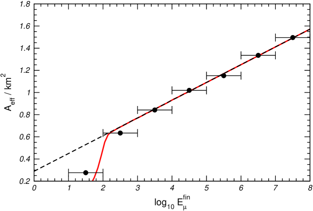
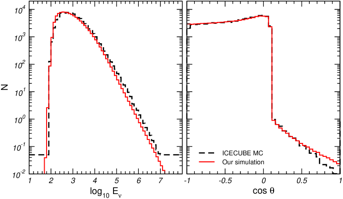
Fig. 2 compares the energy spectrum and the zenith angular distribution of the events in the absence of oscillations after level 2 cuts obtained from our calculation with the results of the experimental MC. In both cases prompt neutrinos are included according to the RQPM model for charm production. The figure illustrates how our simple semianalytical calculation correctly reproduces the experimental simulation.

Figure 2: Spectrum and zenith angular distribution after level 2 cuts for one year exposure obtained from our calculation (full lines) and from the experimental MC (dashed lines) (taken from Figs.2 and 9 of Ref. IceCube ).

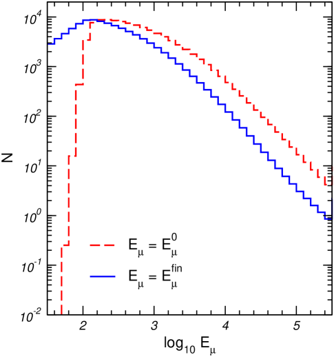
In Fig. 3 we show the expected spectrum of events in the absence of oscillations after level 2 cuts as a function of the muon energy at the detector, $E_{\mu}^{fin}$ (full line). For comparison we also show the spectrum as a function of the muon energy before ranging $E_{\mu}^{0}$. From the figure we read that in 10 years of operation IceCube will collect more than $7\times 10^{5}$ atmospheric neutrino events with energies $E_{\mu}^{fin}>100$ GeV. These events are generated by neutrinos with large enough energy for the standard $\Delta m^{2}$ oscillations to be very much suppressed so they should behave as flavour eigenstates. This high-statistics high-energy event sample offers a unique opportunity to test new physics mechanisms for leptonic flavour mixing as we discuss next.

Figure 3: Expected spectrum of events in the absence of oscillations after level 2 cuts for one year exposure as a function of the muon energy at the detector, $E_{\mu}^{fin}$ (full line). For comparison we also show the spectrum as a function of the initial muon energy $E_{\mu}^{0}$.

III Propagation in Matter of High Energy
Oscillating Neutrinos

As described in the introduction, new physics (NP) scenarios can result in lepton flavour mixing in addition to “standard” $\Delta m^{2}$ oscillations. We concentrate on $\nu_{\mu}$–$\nu_{\tau}$ flavour mixing mechanisms for which the propagation of neutrinos ($+$) and antineutrinos ($-$) is governed by the following Hamiltonian VLICPT2 :

$${\rm H}_{\pm}\equiv\dfrac{\Delta m^{2}}{4E}\mathbf{U}_{\theta}\begin{pmatrix}-1&~{}0\\ \hphantom{-}0&~{}1\end{pmatrix}\mathbf{U}_{\theta}^{\dagger}+\sum_{n}\sigma_{n}^{\pm}\dfrac{\Delta\delta_{n}\,E^{n}}{2}\mathbf{U}_{\xi_{n},\pm\eta_{n}}\begin{pmatrix}-1&~{}0\\ \hphantom{-}0&~{}1\end{pmatrix}\mathbf{U}_{\xi_{n},\pm\eta_{n}}^{\dagger}\;,$$ (11)

where $\Delta m^{2}$ is the mass–squared difference between the two neutrino mass eigenstates, $\sigma_{n}^{\pm}$ accounts for a possible relative sign of the NP effects between neutrinos and antineutrinos and $\Delta\delta_{n}$ parametrizes the size of the NP terms. The matrices $\mathbf{U}_{\theta}$ and $\mathbf{U}_{\xi_{n},\pm\eta_{n}}$ are given by:

$$\mathbf{U}_{\theta}=\begin{pmatrix}\hphantom{-}\cos\theta&~{}\sin\theta\\ -\sin\theta&~{}\cos\theta\end{pmatrix}\,,\qquad\mathbf{U}_{\xi_{n},\pm\eta_{n}}=\begin{pmatrix}\hphantom{-}\cos\xi_{n}\hphantom{e^{-i\eta_{n}}}&~{}\sin\xi_{n}e^{\pm i\eta_{n}}\\ -\sin\xi_{n}e^{\mp i\eta_{n}}&~{}\cos\xi_{n}\hphantom{e^{-i\eta_{n}}}\end{pmatrix}\,;$$ (12)

by $\eta_{n}$ we denote the possible non-vanishing relative phases.

If NP strength is constant along the neutrino trajectory the oscillation probabilities take the form  VLICPT2 :

$$P_{\nu_{\mu}\to\nu_{\mu}}=1-P_{\nu_{\mu}\to\nu_{\tau}}=1-\sin^{2}2\Theta\,\sin^{2}\left(\frac{\Delta m^{2}L}{4E}\,\mathcal{R}\right)\,,$$ (13)

with

$$\sin^{2}2\Theta =\frac{1}{\mathcal{R}^{2}}\left(\sin^{2}2\theta+R_{n}^{2}\sin^{2}2\xi_{n}+2R_{n}\sin 2\theta\sin 2\xi_{n}\cos\eta_{n}\right)\,,$$ (14)

$$\mathcal{R} =\sqrt{1+R_{n}^{2}+2R_{n}\left(\cos 2\theta\cos 2\xi_{n}+\sin 2\theta\sin 2\xi_{n}\cos\eta_{n}\right)}\;,$$ (15)

$$R_{n} =\sigma_{n}^{+}\frac{\Delta\delta_{n}E^{n}}{2}\,\frac{4E}{\Delta m^{2}}\,,$$ (16)

where, for simplicity, we have assumed scenarios with one NP source characterized by a unique $\Delta\delta_{n}$.

Eq. (11) describes, for example, flavour mixing due to new tensor-like interactions for which $n=1$ leading to a contribution to the oscillation wavelength inversely proportional to the neutrino energy. This is the case for $\nu_{\mu}$’s and $\nu_{\tau}$’s of different masses in the presence of violation of the equivalence principle due to non- universal coupling of the neutrinos, $\gamma_{1}\neq\gamma_{2}$ ($\nu_{1}$ and $\nu_{2}$ being related to $\nu_{\mu}$ and $\nu_{\tau}$ by a rotation $\xi_{vep}$), to the local gravitational potential $\phi$ VEP ; VEP1 ; VEPpheno .

For constant potential $\phi$, this mechanism is phenomenologically equivalent to the breakdown of Lorentz invariance resulting from different asymptotic values of the velocity of the neutrinos, $c_{1}\neq c_{2}$, with $\nu_{1}$ and $\nu_{2}$ being related to $\nu_{\mu}$ and $\nu_{\tau}$ by a rotation $\xi_{vli}$ VLI1 ; VLI2 .

For vector-like interactions, $n=0$, the oscillation wavelength is energy-independent. This may arise, for instance, from a non-universal coupling of the neutrinos, $k_{1}\neq k_{2}$ ($\nu_{1}$ and $\nu_{2}$ is related to the $\nu_{\mu}$ and $\nu_{\tau}$ by a rotation $\xi_{Q}$), to a space-time torsion field $Q$ torsion . Violation of CPT resulting from Lorentz-violating effects such as the operator, $\bar{\nu}_{L}^{\alpha}b_{\mu}^{\alpha\beta}\gamma_{\mu}\nu_{L}^{\beta}$, also leads to an energy independent contribution to the oscillation wavelength VLICPT1 ; VLICPT2 ; VLICPT3 which is a function of the eigenvalues of the Lorentz violating CPT-odd operator, $b_{i}$, and the rotation angle, $\xi_{\not\text{CPT}}$, between the corresponding neutrino eigenstates $\nu_{i}$ and the flavour eigenstates $\nu_{\alpha}$.

The flavour oscillations of atmospheric $\nu_{\mu}$’s in this scenarios is described by Eq. (13) with the identification:

$$\xi_{1}=\xi_{vep} \Delta\delta_{1}=2|\phi|(\gamma_{1}-\gamma_{2})\equiv 2|\phi|\Delta\gamma\leq 1.6\times 10^{-24}\,,\qquad{\rm for\,VEP}$$ (17)

$$\xi_{1}=\xi_{vli}\,, \Delta\delta_{1}=(c_{1}-c_{2})\equiv\delta c/c\leq 1.6\times 10^{-24}\,,\qquad{\rm for\,VLI}$$ (18)

$$\xi_{0}=\xi_{Q}\,, \Delta\delta_{0}=Q(k_{1}-k_{2})\leq 6.3\times 10^{-23}~{}\text{GeV}\,,\qquad{\rm for\,coupling\,to\,torsion}$$ (19)

$$\xi_{0}=\xi_{\not\text{CPT}}\,, \Delta\delta_{0}=b_{1}-b_{2}\leq 5.0\times 10^{-23}~{}\text{GeV}\,\,,\qquad{\rm for\,\,\,/\!\!\!\!CPT\,,\,VLI}$$ (20)

where for the first three scenarios $\sigma^{+}=\sigma^{-}$ while for the CPT violating case $\sigma^{+}=-\sigma^{-}$.

At present the strongest limits on NP neutrino oscillations arise from the non-observation of departure from the $\Delta m^{2}$ oscillation behaviour in atmospheric neutrinos at SK and the confirmation of $\nu_{\mu}$ oscillations with the same oscillation parameters from K2K. In Eqs. (17–20) we quote the $3\sigma$ bounds from the up-to-date combined analysis of SK and K2K data performed in Ref. ouratmnp .

For most of the neutrino energies considered here, the standard $\Delta m^{2}$ oscillations are suppressed and the NP effect is directly observed. As a consequence, the results will be independent of the phase $\eta_{n}$ and we can chose the NP parameters in the range

$$~{}\Delta\delta_{n}\geq 0\,, ~{}0\leq\xi_{n}\leq\pi/4\,.$$ (21)

The Hamiltonian of Eq. (11) describes the coherent evolution of the $\nu_{\mu}$–$\nu_{\tau}$ ensemble for any neutrino energy. High-energy neutrinos propagating in the Earth can also interact inelastically with the Earth matter either by charged current and neutral current (NC) and as a consequence the neutrino flux is attenuated. This attenuation is qualitatively and quantitatively different for $\nu_{\tau}$’s and $\nu_{\mu}$’s. Muon neutrinos are absorbed by CC interactions while tau neutrinos are regenerated because they produce a $\tau$ that decays into another tau neutrino before losing energy  hs . As a consequence, for each $\nu_{\tau}$ lost in CC interactions, another $\nu_{\tau}$ appears (degraded in energy) from the $\tau$ decay and the Earth never becomes opaque to $\nu_{\tau}^{\prime}s$. Furthermore, as pointed out in Ref. kolb , a new secondary flux of $\bar{\nu}_{\mu}$’s is also generated in the leptonic decay $\tau\rightarrow\mu\bar{\nu}_{\mu}\nu_{\tau}$.

Attenuation and regeneration effects of incoherent neutrino fluxes can be consistently described by a set of coupled partial integro-differential cascade equations (see for example reno and references therein). In this way, for example, the observed $\nu_{\mu}$ and oscillation-induced $\nu_{\tau}$ fluxes (and the associated event rates in a high energy neutrino telescope) from astrophysical sources has been evaluated. Alternatively, these effects can be accounted for in a Monte Carlo simulation of the neutrino propagation in matter hs ; kolb ; crotty . Whatever the technique used, because of the long distance traveled by the neutrinos from the source, the oscillations average out and the neutrinos arriving at the Earth can be treated as an incoherent superposition of mass eigenstates.

For atmospheric neutrinos this is not the case because oscillation, attenuation, and regeneration effects occur simultaneously when the neutrino beam travels across the Earth’s matter. For the phenomenological analysis of conventional neutrino oscillations this fact can be ignored because the neutrino energies covered by current experiments are low enough for attenuation and regeneration effects to be negligible. Especially for non-standard scenario oscillations, future experiments probe high-energy neutrinos for which the attenuation and regeneration effects have to be accounted for simultaneously. In order to do so, we modify the neutrino flavour oscillation equations and couple them to the $\tau$ evolution equations as described next.

We find it convenient to use the density matrix formalism to describe neutrino flavour oscillations. The evolution of the neutrino ensemble is determined by the Liouville equation for the density matrix $\rho(t)=\nu(t)\otimes\nu(t)^{\dagger}$

$$\frac{d{\rho}}{dt}=-i[{\rm H},{\rho}]\,,$$ (22)

where ${\rm H}$ is given by Eq. (11). The survival probability in Eq. (13) is given by $P_{\mu\mu}(t)={\rm Tr}[\Pi_{\nu_{\mu}}\,\rho(t)]$, where $\Pi_{\nu_{\mu}}=\nu_{\mu}\otimes\nu_{\mu}$ is the $\nu_{\mu}$ state projector, and with initial condition $\rho(0)=\Pi_{\nu_{\mu}}$. An equivalent equation can be written for the antineutrino density matrix.

For the case of oscillations between two neutrino states the hermitian operators $\rho$, ${\rm H}$ and the flavour projectors $\Pi_{\nu_{\mu}}$ and $\Pi_{\nu_{\tau}}$ can be expanded in the basis formed by the unit matrix and the three Pauli matrices $\sigma_{i}$. In particular we can write

$${\rho(t)} = \frac{1}{2}\left(I+\vec{p}(t)\cdot\vec{\sigma}\right)\,,$$ (23)

$${\rm H} = \frac{1}{2}\,\vec{h}\cdot\vec{\sigma}\;,$$

and the evolution of the neutrino ensemble is determined by a precession-like equation of the three-vector $\vec{p}(t)$

$$\frac{d\vec{p}}{dt}\,=\,\vec{p}(t)\,\times\,\vec{h}\,.$$ (24)

In this formalism attenuation effects due to CC and NC interactions can be introduced by relaxing the condition ${\rm Tr}(\rho)=1$. In this case

$$\rho(t)=\frac{1}{2}\left(p_{0}(t)+\vec{p}(t)\cdot\vec{\sigma}\right)\,,$$ (25)

and

$$\frac{d{\rho(E,t)}}{dt}=-i[{\rm H}(E),\rho(E,t)]-\sum_{\alpha}\frac{1}{2\lambda^{\alpha}_{\rm int}(E,t)}\left\{\Pi_{\alpha},\rho(E,t)\right\}\,,$$ (26)

where we have explicitly exhibited the energy dependence and

$$[\lambda^{\alpha}_{int}(E,t)]^{-1}\equiv[\lambda^{\alpha}_{\rm CC}(E,t)]^{-1}+[\lambda_{\rm NC}(E,t)]^{-1}\,,$$

$$[\lambda^{\alpha}_{\rm CC}(E,t)]^{-1}=n_{T}(x)\,\sigma^{\alpha}_{\rm CC}(E)\,,$$ (27)

$$[\lambda_{\rm NC}(E,t)]^{-1}=n_{T}(x)\,\sigma_{\rm NC}(E)\,.$$ (28)

$n_{T}(x)$ is the number density of nucleons at the point $x=ct$. $\sigma^{\alpha}_{\rm CC}(E)$ is the cross section for CC interaction, $\nu_{\alpha}\,+\,N\,\rightarrow\,l_{\alpha}\,+X$, and $\sigma_{\rm NC}(E)$ is the cross section for $\nu_{\alpha}\,+\,N\,\rightarrow\,\nu_{\alpha}\,+X$ which is flavour independent. Thus we obtain four equations that describe the evolution of the neutrino system because one has to take into account both the flavour precession of the vector $\vec{p}(E,t)$ as well as the neutrino intensity attenuation encrypted in the evolution of $p_{0}(E,t)$.

$\nu_{\tau}$ regeneration and neutrino energy degradation can be accounted for by coupling these equations to the shower equations for the $\tau$ flux, $F_{\tau}(E_{\tau},t)$ (we denote by $F$ the differential fluxes $d\phi/(dE\,d\cos\theta)$). For convenience we define the neutrino flux density matrix $F_{\nu}(E,x)=F_{\nu_{\mu}}(E,x_{0})\rho(E,x=c\,t)$ where $F_{\nu_{\mu}}(E,x_{0})$ is the initial neutrino flux. The equations can be written as:

$$\frac{d{F_{\nu}}(E_{\nu},x)}{dx} = -i[{\rm H},F_{\nu}(E_{\nu},x)]-\sum_{\alpha}\frac{1}{2\lambda^{\alpha}_{\rm int}(E_{\nu},x)}\left\{\Pi_{\alpha},F_{\nu}(E_{\nu},x)\right\}$$ (29)

$$+\int_{E_{\nu}}^{\infty}\frac{1}{\lambda_{\rm NC}(E^{\prime}_{\nu},x)}F_{\nu}(E^{\prime}_{\nu},x)\frac{dN_{\rm NC}(E^{\prime}_{\nu},E_{\nu})}{dE_{\nu}}dE^{\prime}_{\nu}$$

$$+\int_{E_{\nu}}^{\infty}\frac{1}{\lambda^{\tau}_{\rm dec}(E_{\tau},x)}F_{\tau}(E_{\tau},x)\frac{dN_{\rm dec}(E_{\tau},E_{\nu})}{dE_{\nu}}dE_{\tau}\,\Pi_{\tau}$$

$$+{\rm Br_{\mu}}\,\int_{E_{\nu}}^{\infty}\frac{1}{\lambda^{\tau}_{\rm dec}(E_{\tau},x)}\,\bar{F}_{\tau}(\bar{E}_{\tau},x)\frac{d\bar{N}_{\rm dec}(\bar{E}_{\tau},E_{\nu})}{dE_{\nu}}d\bar{E}_{\tau}\,\Pi_{\tau}\,,$$

$$\frac{dF_{\tau}(E_{\tau},t)}{d\,x} = -\frac{1}{\lambda^{\tau}_{dec}(E_{\tau},x)}F_{\tau}(E_{\tau},x)$$ (30)

$$+\int_{E_{\tau}}^{\infty}\frac{1}{\lambda^{\tau}_{\rm CC}(E_{\nu},t)}{\rm Tr}[\Pi_{\tau}\,{F_{\nu}}(E_{\nu},t)]\frac{dN_{\rm CC}(E_{\nu},E_{\tau})}{dE_{\tau}}dE_{\nu}\,.$$

$\lambda^{\tau}_{\rm dec}(E_{\tau},x)=\gamma_{\tau}\,c\,\tau_{\tau}$. $\tau_{\tau}$ is the $\tau$ lifetime and $\gamma_{\tau}=E_{\tau}/m_{\tau}$ is its gamma factor.

We have calculated the CC and NC distributions

$$\frac{dN_{\rm NC}(E^{\prime}_{\nu},E_{\nu})}{dE_{\nu}}\equiv\frac{1}{\sigma_{\rm NC}(E^{\prime}_{\nu})}\frac{d\sigma_{\rm NC}(E^{\prime}_{\nu},E_{\nu})}{dE_{\nu}}\,,$$

$$\frac{dN_{\rm CC}(E_{\nu},E_{\tau})}{dE_{\tau}}\equiv\frac{1}{\sigma^{\tau}_{\rm CC}(E_{\nu})}\frac{d\sigma^{\tau}_{\rm CC}(E_{\nu},E_{\tau})}{dE_{\tau}}\,,$$ (31)

using the MRST-g parton distributions pdf , and we have taken the $\tau$ decay distribution $\frac{dN_{\rm dec}(E_{\tau},E_{\nu})}{dE_{\nu}}$ from Ref. reno and $\frac{d\bar{N}_{\rm dec}(\bar{E}_{\tau},E_{\nu})}{dE_{\nu}}$ from Ref. gaisserbook .

The third term in Eq. (29) represents the neutrino regeneration by NC interactions and the fourth term represents the contribution from $\nu_{\tau}$ regeneration, $\nu_{\tau}\rightarrow\tau^{-}\rightarrow\nu_{\tau}$, describing the energy degradation in the process. The secondary $\nu_{\mu}$ flux from $\bar{\nu}_{\tau}$ regeneration, $\bar{\nu}_{\tau}\rightarrow\tau^{+}\rightarrow\bar{\nu}_{\tau}\,\mu^{+}\,\nu_{\mu}$, is described by the last term where we denote by over-bar the energies and fluxes of the $\tau^{+}$. $\rm Br_{\mu}=0.18$ is the branching ratio for this decay. In Eq. (30) the first term gives the loss of taus due to decay and the last term gives the $\tau$ generation due to CC $\nu_{\tau}$ interactions. In writing these equations we have neglected the tau energy loss, which is only relevant at much higher energies.

An equivalent set of equations can be written for the antineutrino flux density matrix and the for the $\tau^{+}$ flux. Both sets of equations are coupled due to the secondary neutrino flux term.

We solve this set of ten coupled evolution equations that describe propagation through the Earth numerically using the matter density profile of the Preliminary Reference Earth Model PREM and obtain the neutrino fluxes in the vicinity of the detector from

$$\frac{d\phi_{\nu_{\alpha}}(E,\theta)}{dE\,d\cos\theta}={\rm Tr}[F_{\nu}(E,L=2R\cos\theta)\,\Pi_{\alpha}]\,.$$ (32)

In Fig. 4 we illustrate the interplay between the different terms in Eqs. (29) and (30). The figure covers the example of VLI-induced oscillations with $\delta c/c=10^{-27}$ and maximal $\xi_{vli}$ mixing. The upper panels show the final $\nu_{\mu}$ and $\nu_{\tau}$ fluxes for vertically upgoing neutrinos after traveling the full length of the Earth for the initial conditions $d{\Phi(\nu_{\mu})_{0}}/{dE_{\nu}}=d{\Phi(\bar{\nu}_{\mu})_{0}}/{dE_{\nu}}\propto E^{-1}$ and $d{\Phi(\nu_{\tau})_{0}}/{dE_{\nu}}=d{\Phi(\bar{\nu}_{\tau})_{0}}/{dE_{\nu}}=0$.

The figure illustrates that the attenuation in the Earth suppresses the neutrino fluxes at higher energies. The effect of the attenuation in the absence of oscillations is given by the dotted thin line in the left panel. Even in the presence of ocillations this effect can be well described by an overall exponential suppression  gaisserbook ; ls both for $\nu_{\mu}$’s and the oscillated $\nu_{\tau}$’s. In other words, we closely reproduce the curve for “oscillation + attenuation” simply by multiplying the initial flux by the oscillation probability and an exponential damping factor:

$$\frac{d\phi_{\nu_{\alpha}}(E,\theta,L=2R\cos\theta)}{dEd\cos\theta}=\frac{d\phi_{\nu_{\mu},0}(E,\theta)}{dEd\cos\theta}\,P_{\mu\alpha}(E,L=2R\cos\theta)\,\exp[-X(\theta)(\sigma_{\rm NC}(E)+\sigma_{\rm CC}^{\alpha}(E))]\,,$$ (33)

where $X(\theta)$ is the column density of the Earth.

The main effect of energy degradation by NC interactions (the third term in Eq. (29)) that is not accounted for in the approximation of Eq.(33) is the increase of the flux in the oscillation minima (the flux does not vanish in the minimum) because higher energy neutrinos end up with lower energy as a consequence of the NC interactions. The difference between the dash-dotted line and the dashed line is due to the interplay between the $\nu_{\tau}$ regeneration effect (fourth term in Eq. (29)) and the flavour oscillations. As a consequence of the first effect, we see in the right upper panel that the $\nu_{\tau}$ flux is enhanced because of the regeneration of higher energy $\nu_{\tau}$’s, $\nu_{\tau}(E)\rightarrow\tau^{-}\rightarrow\nu_{\tau}(E^{\prime}<E)$, that originated from the oscillation of higher energies $\nu_{\mu}$’s. In turn this excess of $\nu_{\tau}$’s produces an excess of $\nu_{\mu}$’s after oscillation which is seen as the difference between the dashed curve and the dash-dotted curve in the left upper panel. Finally the secondary effect of $\bar{\nu}_{\tau}$ regeneration (last term in Eq. (29)), $\bar{\nu}_{\tau}(E)\rightarrow\tau^{+}\,\rightarrow\mu^{+}\,\bar{\nu}_{\tau}\,\nu_{\mu}(E^{\prime}<E)$, results into the larger $\nu_{\mu}$ flux (seen in the left upper panel as the difference between the dashed and the thick full lines). This, in turn, gives an enhancement in the $\nu_{\tau}$ flux after oscillations as seen in the right upper panel.

Figure 4: Vertically upgoing neutrinos after traveling the full length of the Earth taking into account the effects due to VLI oscillations, attenuation in the Earth, $\nu_{\tau}$ regeneration and secondary $\bar{\nu}_{\tau}$ regeneration (see text for details).

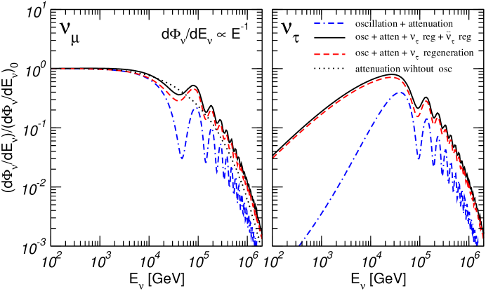
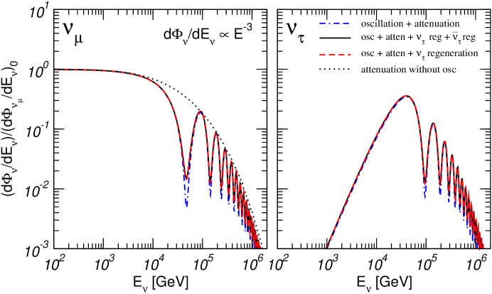
The lower panels show the final $\nu_{\mu}$ and $\nu_{\tau}$ fluxes for an atmospheric-like energy spectrum $d{\Phi(\nu_{\mu})_{0}}/{dE_{\nu}}=d{\Phi(\bar{\nu}_{\mu})_{0}}/{dE_{\nu}}\propto E^{-3}$ and $d{\Phi(\nu_{\tau})_{0}}/{dE_{\nu}}=d{\Phi(\bar{\nu}_{\tau})_{0}}/{dE_{\nu}}=0$. In this case all regeneration effects are suppressed. Regeneration effects result in the degradation of the neutrino energy and the more steeply falling the neutrino energy spectrum, the smaller the contribution to the total flux. Therefore, in this case, the final fluxes can be relatively well described by the approximation in Eq.(33).

IV Example of Physics Reach: VLI-induced Oscillations

Neutrino oscillations introduced by NP effects result in an energy dependent distortion of the zenith angle distribution of atmospheric muon events. We quantify this effect in IceCube by evaluating the expected angular and $E_{\mu}^{fin}$ distributions in the detector using Eq. (II) in conjunction with $\nu_{\mu}$ (and $\bar{\nu}_{\mu}$) fluxes obtained after evolution in the Earth for different sets of NP oscillation parameters.

Together with $\nu_{\mu}$-induced muon events, oscillations also generate $\mu$ events from the CC interactions of the $\nu_{\tau}$ flux which reaches the detector producing a $\tau$ that subsequently decays as $\tau\rightarrow\mu\bar{\nu}_{\mu}\nu_{\tau}$ and produces a $\mu$ in the detector. Using the techniques discussed in the previous sections we compute the number of $\nu_{\tau}$-induced muon events as

$$N^{\nu_{\tau}}_{\rm ev} = T\int^{1}_{-1}d\cos\theta\,\int^{\infty}_{lmin}dl\,\int_{m_{\mu}}^{\infty}dE_{\mu}^{\rm fin}\,\int_{E_{\mu}^{\rm fin}}^{\infty}dE_{\mu}^{0}\,\int_{E_{\mu}^{0}}^{\infty}dE_{\tau}\int_{E_{\tau}}^{\infty}dE_{\nu}$$

$$\frac{d\phi_{\nu_{\tau}}}{dE_{\nu}d\cos\theta}(E_{\nu},\cos\theta)\frac{d\sigma^{\mu}_{CC}}{dE_{\tau}}(E_{\nu},E_{\tau})\,n_{T}\,\frac{dN_{dec}}{dE_{\mu}^{0}}(E_{\tau},E_{\mu}^{0})F(E^{0}_{\mu},E_{\mu}^{\rm fin},l)\,A^{0}_{eff}\,\;,$$

where $\frac{dN_{\rm dec}(E_{\tau},E_{\mu}^{0})}{dE_{\mu}^{0}}$ can be found in Ref. gaisserbook . Equivalently we compute the number of $\bar{\nu}_{\tau}$-induced muon events.

Figure 5: Zenith angle distributions for muon induced events for different values of the VLI parameter $\delta c/c$ and maximal mixing $\xi_{vli}=\pi/4$ for different threshold energy $E_{\mu}^{fin}>E_{\rm threshold}$ normalized to the expectations for pure $\Delta m^{2}$ oscillations . The dashed line includes only the $\nu_{\mu}$-induced muon events and the full line includes both the $\nu_{\mu}$-induced and $\nu_{\tau}$-induced muon events.

For illustration we concentrate on oscillations resulting from VLI that lead to an oscillation wavelength inversely proportional to the neutrino energy. The results can be directly applied to oscillations due to VEP.

We show in Fig. 5 the zenith angle distributions for muon induced events for different values of the VLI parameter $\delta c/c$ and maximal mixing $\xi_{vli}=\pi/4$ for different threshold energy $E_{\mu}^{fin}>E_{\rm threshold}$ normalized to the expectations for pure $\Delta m^{2}$ oscillations. The full lines include both the $\nu_{\mu}$-induced events (Eq.(II)) and $\nu_{\tau}$-induced events (Eq.(IV)) while the last ones are not included in the dashed curves. We see that for a given value of $\delta c/c$ there is a range of energy for which the angular distortion is maximal. Above that energy, the oscillations average out and result in a constant suppression of the number of events. Inclusion of the $\nu_{\tau}$-induced events events leads to an overall increase of the event rate but slightly reduces the angular distortion (see also Fig. 6) as a consequence of the “anti-oscillations” of the $\nu_{\tau}$’s as compared to the $\nu_{\mu}$’s.

In order to quantify the energy-dependent angular distortion we define the vertical-to-horizontal double ratio

$$R_{h/v}(E_{\mu}^{fin,i})\equiv\frac{P_{\rm hor}}{P_{\rm ver}}(E_{\mu}^{fin,i})=\frac{\frac{\displaystyle N^{vli}_{\mu}(E_{\mu}^{fin,i},-0.6<\cos\theta<-0.2)}{\displaystyle N^{no-vli}_{\mu}(E_{\mu}^{fin,i},-0.6<\cos\theta<-0.2)}}{\frac{\displaystyle N^{vli}_{\mu}(E_{\mu}^{fin,i},-1<\cos\theta<-0.6)}{\displaystyle N^{no-vli}_{\mu}(E_{\mu}^{fin,i},-1<\cos\theta<-0.6)}}\;,$$ (35)

where by $E_{\mu}^{fin,i}$ we denote integration in an energy bin of width $0.2\,\log_{10}(E_{\mu}^{fin,i})$ using that IceCube measures energy to 20% in $\log_{10}E$ for muons.

In what follows we will use the double ratio in Eq. (35) as the observable to determine the sensitivity of IceCube to NP-induced oscillations. We have chosen a double ratio to eliminate uncertainties associated with the overall normalization of the atmospheric fluxes at high energies.

Also, in the definition of the double ratio we have conservatively included only events well below the horizon $\cos\theta<-0.2$ to avoid the possible contamination from missreconstructed atmospheric muons which can still survive after level 2 cuts in the angular bins closer to the horizon  IceCube .

Figure 6: The predicted horizontal-to-vertical double ratio in Eq.(35) for different values of $\delta c/c$. The data points in the figure show the expected statistical error corresponding to the observation of no NP effects in 10 years of IceCube.

In Fig. 6 we plot the expected value of this ratio for different values of $\delta c/c$. As mentioned above, IceCube measures energy to 20% in $\log_{10}E$ for muons. Accordingly, we have divided the data in 16 $E_{\mu}^{fin}$ bins: 15 bins between $10^{2}$ and $10^{5}$ GeV and one containing all events above $10^{5}$ GeV. In the figure the full lines include both the $\nu_{\mu}$-induced events (Eq.(II)) and $\nu_{\tau}$-induced events (Eq.(IV)) while the last ones are not included in the dashed curves. As described above, the net result of including the $\nu_{\tau}$-induced events is a slight decrease of the maximum expected value of the double ratio. The data points in the figure show the expected statistical error corresponding to the observation of no NP effects in 10 years of IceCube.

In order to estimate the expected sensitivity we assume that no NP effect is observed and define a simple $\chi^{2}$ function as

$$\chi^{2}(\delta c/c,\xi_{\rm vli})=\sum_{i=1}^{16}\frac{(R_{h/v}(E_{\mu}^{fin,i},\delta c/c,\xi_{\rm vli})-1)^{2}}{\sigma_{\rm stat,i}^{2}}\,$$ (36)

where $\sigma_{\rm stat,i}$ is computed from the expected number of events in the absence of NP effects (see Table 1).

	RPQM		TIG
$\log_{10}(E_{\mu}^{fin})$	$-1\leq\cos\theta\leq-0.6$	$-0.6\leq\cos\theta\leq-0.2$	$-1\leq\cos\theta\leq-0.6$	$-0.6\leq\cos\theta\leq-0.2$
2.00– 2.20	52474	61806	51427	60920
2.20– 2.40	46234	55598	44987	54539
2.40– 2.60	35965	44586	34634	43422
2.60– 2.80	26001	33588	24647	32415
2.80– 3.00	17358	23400	16107	22294
3.00– 3.20	10710	15126	9630	14141
3.20– 3.40	6172	9054	5320	8250
3.40– 3.60	3330	5099	2701	4494
3.60– 3.80	1721	2722	1289	2291
3.80– 4.00	856	1388	578	1098
4.00– 4.20	410	685	242	498
4.20– 4.40	191	330	96	215
4.40– 4.60	86	156	36	89
4.60– 4.80	38	74	13	36
4.80– 5.00	16	34	5	14
5.00– 9.00	10	28	2	8

Table 1: Number of expected atmospheric $\nu_{\mu}$-induced muon events in 10 years of IceCube operaton in the different energy bins and angular bins used in the analysis, assuming no NP effect is observed.

We show in Fig. 7 the sensitivity limits in the $[\delta c/c,\xi_{\rm vli}]$-plane at 90, 95, 99 and 3 $\sigma$ CL obtained from the condition $\chi^{2}(\delta c/c,\xi_{\rm vli})<\chi^{2}_{max}({\rm CL,2dof})$. In order to estimate the uncertainty associated with the poorly known prompt neutrino fluxes we show in the figure the results obtained using the RQPM model (filled regions) and the TIG model (full lines). The difference is about 50% in the strongest bound on $\delta c/c$.

Figure 7: Sensitivity limits in the $\delta c/c,\xi_{\rm vli}$ at 90, 95, 99 and 3 $\sigma$ CL. The hatched area in the upper right corner is the present $3\sigma$ bound from the analysis of SK data in Ref. ouratmnp .

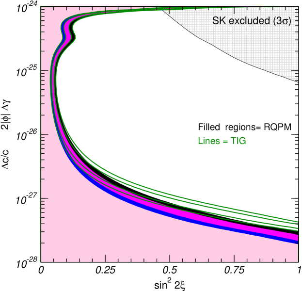
The figure illustrates the improvement on the present bounds by more than two orders of magnitude even within the context of this very conservative analysis. The loss of sensitivity at large $\delta c/c$ is a consequence of the use of a double ratio as an observable. Such an observable is insensitive to NP effects if $\delta c/c$ is large enough for the oscillations to be always averaged leading only to an overall suppression.

When data becomes available a more realistic analysis is likely to lead to a further improvement of the sensitivity.

V Summary

In this paper we have investigated the physics that can be probed with the high-statistics high-energy data on atmospheric neutrinos which will be collected by the IceCube detector. In order to do so first we have developed a semianalytical simulation of the detector performance. In particular, we present in Eqs. (2)–(10) the parametrization of the effective area of the detector which correctly reproduces the results of the detailed experimental MC for the response of the IceCube detector after events that are not neutrinos have been rejected using the quality cuts referred to as level 2 cuts. We conclude that in 10 years of operation IceCube will collect more than 700 thousand atmospheric neutrino events with energies $E_{\mu}^{fin}>100$ GeV which offer a unique opportunity to test new physics mechanisms for leptonic flavour mixing which are not suppressed at high energy. In general these effects are expected to induce an energy dependent angular distortion of the events.

Next, because of the relatively high energy of the neutrino sample, NP induced flavour oscillations, propagation in the Earth, regeneration of neutrinos due to $\tau$ decay must be treated in a consistent way. In Sec. III we have presented the corresponding evolution equations. We conclude that for steeply falling neutrino energy spectra, such as the atmospheric neutrino one, the dominant effect together with flavour oscillations is the attenuation of the oscillation amplitude due to inelastic CC and NC interactions of the neutrinos in the Earth in conjunction with the production $\nu_{\tau}$-induced muon events due to the chain $\nu_{\tau}\rightarrow\tau\rightarrow\mu\nu_{\mu}\nu_{\tau}$ in the vicinity of the detector. $\nu_{\tau}$-induced muon events can increase the event sample by at most ${\cal O}(10\%)$.

Finally we have applied these results to realistically evaluate the reach of IceCube in studying physics beyond conventional neutrino oscillations induced by violation of Lorentz invariance and/or the equivalence principle. In Fig. 7 we show how even with a very conservative analysis the range of testable sizes of these effects can be easily extended by more than two orders of magnitude. The methods developed are readily applicable to probe speculations on other non-conventional physics associated with neutrinos.