1 Introduction and overview

In this paper we investigate the role that dissipation can play in biasing vacuum selection after a symmetry breaking phase transition. Our work was initially motivated by a mechanism suggested by Nagasawa and Brandenberger [1] to stabilise non-topological classical solutions by out-of-equilibrium effects. They studied an $O(4)$ model in which charged and neutral scalars coupled differently to a thermalised photon bath. Under the assumption that only the charged fields receive thermal corrections from the bath, these authors argued that the vacuum manifold would collapse from $S^{3}$ to $S^{1}$ and therefore temporarily stabilise non-topological strings.

The analysis in [1] is focused on the stability of embedded strings when immersed in a thermalised plasma. However, the primordial question of whether the formation of the defect is dynamically favoured has never been addressed. By looking at the requirements that favour their formation we found a close link between “external” dissipation and vacuum selection that ranges beyond our initial aim. By external we mean a source of dissipation that is not related to the interactions between the system and the heat bath.

The vacuum selection we discuss can take place in the early universe and in heavy-ion collisions. In the early universe, the most relevant areas for applications are in the studies of preheating at the end of inflation [2] and defect formation in non-equilibrium cosmological phase transitions [3].

Current and future heavy-ion collision experiments also provide scenarios where dissipative vacuum selection might take place. A specific problem where this process might occur is the formation of disoriented chiral condensates [4, 5]. Processes of similar nature might take place in the quark-gluon plasma where modes with different thermalisation times coexist. However, our study, which is based on a symmetry breaking, does not provide by itself a mechanism for this case.

The mechanism we investigate is illustrated here for the same $O(4)$ scalar field theory in $3+1$ dimensions used in [1]. Some general assumptions are required to specify the properties of the model but when presented out of a particular context, at first sight, these might not appear natural. Therefore, we think it convenient to start with a brief outline of our study. In the context of our work we see the field theory as an effective model for the soft long-wavelength modes of a system coupled to a heat bath. At low temperatures the system has a symmetry broken phase and the symmetry is restored above some finite temperature $T_{c}$.

The following are key requirements concerning the coupling of the scalar fields to the heat bath. In the ordered phase, two of the scalar fields, say for definiteness $\phi_{1,2}$, have decoupled from the heat bath, while the remaining fields, say $\phi_{3,4}$, stay coupled. This situation is more natural than it seems at first sight. For example it occurs when the fields $\phi_{1,2}$ are neutral and $\phi_{3,4}$ are charged, both with respect to the same conserved charge, and the heat bath consists predominantly of quanta of the associated gauge field.

Furthermore, the coupling between $\phi_{3,4}$ and the bath is assumed to be much stronger than the scalar self-coupling. Then, we expect that by the time $\phi_{3,4}$ thermalise at the heat bath temperature $T<T_{c}$, the $\phi_{1,2}$ fields are still out of equilibrium. In other words, the relative strength of the couplings implies that the relaxation times of $\phi_{3,4}$ are much smaller than the ones of $\phi_{1,2}$. This is a condition that can be realised in the early universe. The less favourable transition is probably the most recent one, the chiral symmetry breaking transition, because of the strong pion interactions. Under these circumstances, when some fields are coupled and other uncoupled to a heat bath, the question then arises: What is the effective vacuum manifold in this system?

When all the fields are coupled to the heat bath and dissipate according to the fluctuation-dissipation relation the answer is well known. The vacuum manifold is the three-sphere $S^{3}$ covered by all the equivalent scalar configurations that minimise the free energy. The soft modes described by the fields do not form a closed system because their energy is being exchanged with the heat bath, e.g. via collisions and decay channels, giving origin to dissipation. Let us assume, as it is normally the case, that these terms are characterised by viscosity coefficients $\eta_{i}$ associated with each scalar $\phi_{i}$.

The situation we study here differs in two ways. First, the neutral fields are not coupled directly to a heat bath. Second, and most importantly, we consider these decoupled fields to have “external” sources of dissipation. For example, in a cosmological context this type of dissipation is naturally associated with the expansion of the universe. As a result the decoupled $\phi_{1,2}$ fields stabilise in steady states that can be characterised by an effective temperature $T_{\mathrm{eff}}<T$, independently on whether these fields condense or not.

The most interesting effect occurs when the “external” dissipation is much smaller than the dissipation in the coupled fields due to their interaction with the bath. We would expect a small external dissipation to have only a negligible effect on the evolution of the fields. However, this is in general not the case. We have that at vanishing scalar self-coupling the limit $\eta_{1,2}\to 0$, i.e. the “external” sources of dissipation are “switched off”, is singular. This has the effect of changing the symmetry breaking pattern even for small values of $\eta_{1,2}$. In this limit the neutral fields are selected to condense, therefore effectively reducing the vacuum manifold from $S^{3}$ to $S^{1}$ as originally suggested by Nagasawa and Brandenberger [1].

In reality, the uncoupled fields are still receiving energy from the bath and the role of the external dissipation is simply to release this energy at a comparable rate. This rate is much smaller than the corresponding values for the coupled fields and has no appreciable effect on them.

The origin of the vacuum manifold reduction in our analysis is identified without having to call for out-of-equilibrium effects as in [1]. We emphasise the important role played by the existence of different steady states for the various fields due to the “external” source of dissipation.

The vacuum selection takes place above a small critical dissipation which occurs when the neutral fields stabilise at a “cold” enough $T_{\mathrm{eff}}$. Our conclusions, therefore, is that the reduction is more widely applicable than previously thought.

Our simulations are governed by phenomenological Langevin equations describing the dynamical evolution of the fields. These equations have been previously used in a relativistic context to study non-equilibrium phenomena in cosmological phase transition [6, 7, 8]. There are known limitations to the use of these equations which we discuss in Sect. 4 and 5. They provide nevertheless an economic and qualitative good description of the different processes involved in the dynamic evolution of the fields where the coupling to the heat bath is expressed by rapidly fluctuating fields and the dissipation effects are expressed by viscosity terms. In particular, this makes it easy to analyse the effects of dissipation terms that are not related to interactions with the heat bath.

The paper is organised as follows. In Sect. 2, we discuss the role of decoupling and dissipation in the vacuum biasing mechanism. A toy model illustrating the dissipation requirement in a solvable system is presented in Sect. 3. We illustrate in this simple case the effects of non thermal dissipation terms that are not related to exchanges with a heat bath but originate for example from the expansion of the system. In Sect. 4 we study dissipative vacuum selection in the $O(4)$ symmetric model in 3+1 dimensions. This section is divided in four subsections. We begin with a discussion on the use of phenomenological Langevin equations. The results of our simulations are then presented in Sect. 4.2 and in Sect. 4.3 we analyse the effect of varying the parameters of the model. Finally, in Sect. 4.4 we discuss the conditions that guarantee the vacuum selection to be in place when all fluctuating (and dissipative) contributions are accounted for. We end in Sect. 5 with a summary and a discussion of future work.

2 Decoupling and dissipation

We analyse the field dynamics in a system that undergoes a symmetry breaking transition and where different fields sectors in the system reach distinct “thermalised” states with some heat bath. The nature of the bath will be characterised below. Some fields arrive at a standard thermalised state at the temperature of the bath after a relatively short relaxation time. The remaining fields stay out of equilibrium for a longer period, which can still be small compared to observation times. The fields that take longer to either thermalise or reach another type of equilibrium state are weakly or indirectly coupled to a heat bath. We refer to them as decoupled in a convenient loose sense that will be made clear later. In particular, we are interested in the situation where the decoupled fields condense following a finite temperature phase transition. In order for this to happen these fields must lose most of their energy and for this reason we will follow closely the role of dissipation.

In order to discuss a setting where this scenario can be realised we use an $O(4)$ linear sigma model Lagrangean,

$${\mathcal{L}}=\frac{1}{2}\ \partial_{\mu}\phi_{i}\partial^{\mu}\phi_{i}\ -\frac{\lambda}{4}\left(\phi_{i}\phi_{i}-v^{2}\right)^{2}\!,\ i=1,2,3,4,$$ (1)

to describe the propagation and self-interactions of soft modes. For convenience, we consider $\phi_{1}$ and $\phi_{2}$ to be neutral scalars and $\phi_{3}$ and $\phi_{4}$ to be the constituents of a charged scalar $\phi^{\pm}=(\phi_{3}\pm i\phi_{4})/\sqrt{2}$ with respect to a $U(1)$ charge. For concreteness let it be $U(1)_{\mathrm{EM}}$. Therefore, $\phi^{\pm}$ is coupled to a bath of photons while the neutral scalars are not. In a more comprehensive analysis the effects of the fluctuations from the hard modes of the scalar fields are also to be taken into account. We will discuss their effects in the next sections.

By keeping the model simple we can aim at a better understanding on how a small dissipation can play a role in selecting the vacuum. This is the effect we wish to emphasise and alongside we lay the conditions under which the vacuum manifold shows the selectiveness that favours the formation of such embedded structures.

Throughout this paper we work under the assumption that the coupling between the charged scalars and the photon bath is much stronger than the scalar self-coupling. Without this assumption leading to an effective separation of scales no non-trivial selection seems to take place. With these conditions, we expect the charged scalars to thermalise “quickly”. Their relaxation time sets the scale for what we will refer as a quick thermalisation time. In practice, at the observation scale, the charged scalars can be said to remain in equilibrium. The neutral scalars have of course a longer thermalisation time and are at least close to thermal equilibrium.

One of our aims is to express quantitatively the distinction between the steady state reached by the neutral and the charged fields. If the decoupled fields have no direct process to dissipate their energy they reach a thermal equilibrium state at the temperature $T$ of the photon bath. This thermalisation occurs because the decoupled fields are not completely cut off from the photon bath due to the quartic scalar self-interaction. The rate at which the neutral fields thermalise depends on the strength of $\lambda$. Elsewise, if they dissipate due to the expansion of the system as it cools, as in the early universe or heavy-ion collisions, the steady state they reach is “colder”. This effect leads to their selective condensation and suggests the use of an effective temperature $T_{\mathrm{eff}}$ as a way to parametrise the distinct steady states. We will present a detailed discussion of $T_{\mathrm{eff}}$ in the next sections.

Before ending this section we refer the reader to the further underlying view that the Lagrangean (1) is better suited for the broken phase. Our model can be seen as a sector in a larger theory. For instance above $T_{c}$ other mediating bosons that decouple at the transition can be responsible for maintaining all the scalars in thermal equilibrium. A known example that inspires this view can be found in the electroweak transition. In this case the $W$- and $Z$-bosons become massive below the transition while the photons remain massless through the transition.

Renormalisation due to radiative and thermal corrections coming from hard modes could also have been included in (1) but this should not have a major effect in our phenomenological analysis. More important are the fluctuation-dissipation effects coming from the scalar hard modes. They do indeed have some effect in the main simple picture laid down in this section but they do not change the outcome if the relatively magnitudes of the couplings remains as assumed above as we show at the end of the next section.

Before we address the dynamical description of the model described by (1) we look at a simple two particle system where we can perform analytic calculations that highlight the main features of the “vacuum biasing”.

3 Biasing in a two field system in zero dimensions

In this section we illustrate how decoupling and dissipation combine to bias the distribution of energy in a toy system. We have two coupled one-dimensional oscillators of unit mass and restoring constants $m^{2}_{0}$ and $m^{2}_{c}$. Alternatively, they can be interpreted as two interacting fields in zero spatial dimensions. The system can be seen as a first approximation for an effective model for the zero Fourier components of a field theory in three spatial dimensions. It is a simplified version of the $O(4)$ model introduced in the previous section, but now with only two fields. Here one “charged” field $\phi_{c}$ is coupled to a heat bath, and the other “neutral” field $\phi_{0}$ is not coupled.

We adopt a Langevin description, in analogy to what we will do in the next section for the system described by (1), where the coupling to the bath is represented by a random rapidly varying field. In a canonical form the equations of motion are,

$$\dot{\phi}_{0} = \pi_{0}$$

$$\dot{\pi}_{0} = -\eta_{0}\pi_{0}-m_{0}^{2}\phi_{0}-\frac{\partial V}{\partial\phi_{0}}$$

$$\dot{\phi}_{c} = \pi_{c}$$

$$\dot{\pi}_{c} = -\eta_{c}\pi_{c}-m_{c}^{2}\phi_{c}-\frac{\partial V}{\partial\phi_{c}}+\xi.$$ (2)

The interaction between the fields is contained in the potential $V(\phi_{0},\phi_{c})$ and the dissipation is expressed by the viscosity terms involving the coefficients $\eta_{0}$ and $\eta_{c}$. The interaction of the charged field, $\phi_{c}$, with the “photon” bath is modeled by the random field $\xi$,

$$\langle\xi(t)\rangle=0,\,\,\,\,\,\,\,\,\,\langle\xi(t)\xi(t^{\prime})\rangle=\Omega\delta(t-t^{\prime}),$$ (3)

where $\Omega$ is the variance of the Gaussian white noise. This ensemble of fields can be described by the probability density $\rho(\phi_{0},\pi_{0},\phi_{c},\pi_{c},t)$. The evolution of this distribution is governed by the Fokker-Planck type equation,

$$\frac{\partial\rho}{\partial t} = -\pi_{0}\frac{\partial\rho}{\partial\phi_{0}}+\Big{(}m_{0}^{2}\phi_{0}+\frac{\partial{V}}{\partial\phi_{0}}\Big{)}\frac{\partial\rho}{\partial\pi_{0}}+\eta_{0}\frac{\partial(\pi_{0}\rho)}{\partial\pi_{0}}-$$ (4)

$$-\pi_{c}\frac{\partial\rho}{\partial\phi_{c}}+\Big{(}m_{c}^{2}\phi_{c}+\frac{\partial{V}}{\partial\phi_{c}}\Big{)}\frac{\partial\rho}{\partial\pi_{c}}+\eta_{c}\frac{\partial(\pi_{c}\rho)}{\partial\pi_{c}}+\frac{\Omega}{2}\frac{\partial^{2}\rho}{\partial\pi_{c}^{2}}\ .$$

For any physical observable $A(\phi_{0},\pi_{0},\phi_{c},\pi_{c})$ we have

$$\langle A\rangle(t)=\int d\phi_{0}d\pi_{0}d\phi_{c}d\pi_{c}\ A(\phi_{0},\pi_{0},\phi_{c},\pi_{c})\rho(\phi_{0},\pi_{0},\phi_{c},\pi_{c},t),$$ (5)

and its time derivative can be calculated using equation (4) and integrating by parts. The equation of motion for $\langle A\rangle$ then reads

$$\frac{\partial\langle A\rangle}{\partial t} = \langle\pi_{0}\frac{\partial A}{\partial\phi_{0}}\rangle-\langle\frac{\partial{V}}{\partial\phi_{0}}\frac{\partial A}{\partial\pi_{0}}\rangle-m_{0}^{2}\,\langle\phi_{0}\frac{\partial A}{\partial\pi_{0}}\rangle-\eta_{0}\,\langle\pi_{0}\frac{\partial A}{\partial\pi_{0}}\rangle+\langle\pi_{c}\frac{\partial A}{\partial\phi_{c}}\rangle-$$ (6)

$$- \langle\frac{\partial{V}}{\partial\phi_{c}}\frac{\partial A}{\partial\pi_{c}}\rangle-m_{c}^{2}\,\langle\phi_{c}\frac{\partial A}{\partial\pi_{c}}\rangle-\eta_{c}\,\langle\pi_{c}\frac{\partial A}{\partial\pi_{c}}\rangle+\frac{\Omega}{2}\,\langle\frac{\partial^{2}A}{\partial\pi_{c}^{2}}\rangle.$$

In equilibrium we have $\partial_{t}\langle A\rangle=0$ for all physical observables $A$. One way of obtaining a full description of the system in equilibrium is to obtain all the expectation values of all combinations of powers of the four quantities $\phi_{0}$, $\pi_{0}$, $\phi_{c}$ and $\pi_{c}$. These are the $N$-point functions for (classical)-fields in equilibrium. It is easy to see that except for the simple case of quadratic potentials (where we expect the system to be solvable), these equations mix correlations of powers of different degrees in the dynamical variables. This leads to an infinite number of linked equations similar to the Dyson-Schwinger hierarchy. Here we will consider only the quadratic case and take the interaction potential to be

$$V(\phi_{0},\phi_{c})=\lambda\phi_{0}\phi_{c}.$$ (7)

This choice will enable us to carry an analytic treatment. For the case with a quartic interaction $\lambda\phi_{0}^{2}\phi^{2}_{c}$ we have checked that the main features of the results are the same.

For the potential (7), the second order correlation functions with $i\neq j$ satisfy the following system of 10 equations,

$$\phi_{i}^{2} \rightarrow \langle\phi_{i}\pi_{i}\rangle=0\,,\ \ \ \phi_{0}\phi_{c}\ \ \rightarrow\ \ \langle\phi_{c}\pi_{0}\rangle+\langle\phi_{0}\pi_{c}\rangle=0$$

$$\pi_{i}^{2} \rightarrow \lambda\langle\pi_{i}\phi_{j}\rangle+m_{i}^{2}\langle\phi_{i}\pi_{i}\rangle+\eta_{i}\langle\pi_{i}^{2}\rangle-\delta_{i2}\Omega/2=0$$

$$\pi_{0}\pi_{c} \rightarrow \lambda(\langle\phi_{c}\pi_{c}\rangle+\langle\phi_{0}\pi_{0}\rangle)+m_{0}^{2}\langle\phi_{0}\pi_{c}\rangle+m_{c}^{2}\langle\phi_{c}\pi_{0}\rangle+(\eta_{0}-\eta_{c})\langle\pi_{0}\pi_{c}\rangle=0$$

$$\phi_{i}\pi_{i} \rightarrow \lambda\langle\phi_{i}\phi_{j}\rangle+m_{i}^{2}\langle\phi_{i}^{2}\rangle+\eta_{i}\langle\phi_{i}\pi_{i}\rangle-\langle\pi_{i}^{2}\rangle=0$$

$$\phi_{i}\pi_{j} \rightarrow \lambda\langle\phi_{i}^{2}\rangle+m_{j}^{2}\langle\phi_{i}\phi_{j}\rangle+\eta_{j}\langle\phi_{i}\pi_{j}\rangle-\langle\pi_{i}\pi_{j}\rangle=0\ ,$$ (8)

which is closed because it involves only expectation values of degree two in the dynamical variables. After some work we can solve it obtaining the average for the momentum of the decoupled field,

$$\langle\pi_{0}^{2}\rangle=\frac{\lambda^{2}\Omega}{2}\left[\frac{\eta_{0}\eta_{c}(m_{c}^{2}-m_{0}^{2})^{2}}{(\eta_{0}+\eta_{c})}+\lambda^{2}(\eta_{0}+\eta_{c})+\eta_{0}\eta_{c}(\eta_{c}m_{0}^{2}+\eta_{0}m_{c}^{2})\right]^{-1}.\\$$

In the simpler case when $m_{0}=m_{c}=m$ this reduces to

$$\langle\pi_{0}^{2}\rangle=\frac{\lambda^{2}\Omega}{2(\eta_{0}+\eta_{c})(\lambda^{2}+m^{2}\eta_{0}\eta_{c})}\ .$$ (9)

The other momentum is related to this one by

$$\langle\pi_{c}^{2}\rangle=\frac{\Omega}{2\eta_{c}}-\frac{\eta_{0}}{\eta_{c}}\langle\pi_{0}^{2}\rangle.$$ (10)

Next we assume that the dissipation for the coupled field and the amplitude of the noise obey the fluctuation-dissipation relation, $\Omega=2\eta_{c}T$, where $T$ is the temperature of the bath. We now define the effective stabilisation temperatures

$$T_{\mathrm{eff}}=\langle\pi_{0}^{2}\rangle = \frac{\lambda^{2}\eta_{c}T}{(\eta_{0}+\eta_{c})(\lambda^{2}+m^{2}\eta_{0}\eta_{c})}\ ,$$

$$T^{\prime}_{\mathrm{eff}}=\langle\pi_{c}^{2}\rangle = T-\frac{\eta_{0}}{\eta_{c}}\langle\pi_{0}^{2}\rangle.$$ (11)

for the neutral and charged field respectively. In the case of zero dissipation coefficient for the neutral field, $\eta_{0}=0$, not only these temperatures are the same but also $T_{\mathrm{eff}}=T^{\prime}_{\mathrm{eff}}=T$ for any finite non vanishing values of $\lambda$. On the other hand, when $\eta_{0}>0$ the effective temperatures of the asymptotic states of each field are different which justifies using the quantities defined by (3) as convenient parameters to express quantitatively the distinct steady states. We note that similar definitions have been introduced in glassy systems [9], however the $T_{\mathrm{eff}}$ we use here are constants as they refer to steady states after relaxation instead of long lasting transient states.

In this toy model the biasing mechanism corresponds to an unequal distribution of the kinetic energy between the different types of fields. The main features that characterise it are easy to identify from equations (3). To start with, note that if $\eta_{0}\ll\eta_{c}$, $T^{\prime}_{\mathrm{eff}}$ is hardly affected with relation to its value at $\eta_{0}=0$, whereas $T_{\mathrm{eff}}$ can be noticeably reduced, provided $\lambda^{2}\lesssim m^{2}\eta_{0}\eta_{c}$. When these two conditions are simultaneously satisfied even a very small value of the ratio $\eta=\eta_{0}/\eta_{c}$ can cause a large effect on the asymptotic configuration of the uncharged fields $\phi_{0}$. We have verified that simulations for a model with quartic self-interactions indicate the existence of analogous relations.

The reason why a small value of $\eta$ is able to lead to a qualitatively different behaviour is the existence of a singularity to which we now turn our attention. Consider the two sequences of limits, $\lambda\to 0$ followed by $\eta_{0}\to 0$ and its reverse when $\eta_{0}$ is taken to zero first. In the former we have $T_{\mathrm{eff}}\to 0$ and $T^{\prime}_{\mathrm{eff}}\to T$, and in the latter both $T_{\mathrm{eff}}$ and $T^{\prime}_{\mathrm{eff}}$ approach $T$. Clearly, the phenomena that we are studying corresponds to a regime along the first sequence of limits where the two types of fields are weakly coupled to each other but a dissipation in the neutral field prevails even after the self-coupling is “switched-off”. Therefore, we are not only considering $\eta$ small but also $\lambda$ has to be “small” in the sense that

$$\frac{\lambda^{2}}{m^{2}\eta_{c}^{2}}\lesssim\eta=\frac{\eta_{0}}{\eta_{c}}\ll 1.$$ (12)

We might expect that the physical origin of the sizeable effect for small $\eta$ follows from $\eta_{0}$ not being associated with fluctuation-dissipation effects. But this by itself is not sufficient to explain what we observe. Equally important is the existence of at least two scales in the problem. In order to clarify this point let us consider the case when the neutral field also evolves under the effect of fluctuations. To this end we modify the second equation in (3) which now reads

$$\dot{\pi}_{0}=-\eta_{0}\pi_{0}-m_{0}^{2}\phi_{0}-\frac{\partial V}{\partial\phi_{0}}+\xi_{0},$$ (13)

where the dissipation coefficient $\eta_{0}$ is now decomposed into two terms, $\eta_{0}=\eta^{\mathrm{ext}}_{0}+\eta^{\mathrm{fl}}_{0}$. The first term corresponds to an external source of dissipation while the second one is related to fluctuating forces according to a standard fluctuation-dissipation relation,

$$\langle\xi^{\mathrm{fl}}_{0}(t)\rangle=0,\,\,\,\,\,\,\,\,\,\langle\xi^{\mathrm{fl}}_{0}(t)\xi^{\mathrm{fl}}_{0}(t^{\prime})\rangle=\Omega_{0}\delta(t-t^{\prime}),$$ (14)

where $\Omega_{0}=2\eta^{\mathrm{fl}}_{0}T_{0}$, with $T_{0}$ the temperature of the bath coupled to the neutral field. It is natural in a first approximation to take $T_{0}=T$ as we should not expect a selective behaviour for the high energy modes. Moreover, this situation corresponds to a case where biasing is less favourable. The strength of the coupling of each field to the heat bath reflects itself in the relative magnitudes of the dissipation coefficients. This matter will be made clearer in the full $O(4)$ model.

A generalisation of the calculation leading to (3) including the noise for the neutral fields and with $T_{0}=T$ gives

$$\frac{T^{\prime}_{\mathrm{eff}}-T_{\mathrm{eff}}}{T}=\frac{\eta^{\mathrm{ext}}_{0}}{\eta_{0}}f(m^{2}\eta_{c}\eta_{0}/\lambda^{2}),$$ (15)

with $f(x)=x/(1+x)$, from which we see that the effective temperatures of the steady states can still differ substantially if in addition to (12) we have $\eta^{\mathrm{ext}}_{0}\sim\eta_{0}$. These combine to guarantee that the argument of $f$ is large therefore assuring that $f\sim 1$. Under these conditions $T^{\prime}_{\mathrm{eff}}-T_{\mathrm{eff}}\sim T$.

Note that an external dissipation should for consistency affect both fields. The inclusion of such non-thermal dissipation in the equations of the charged fields adds a new term in the right-hand side of (15), analogous to the present one, where for instance the prefactor is now $\eta^{\mathrm{ext}}_{c}/\eta_{c}$ instead of $\eta^{\mathrm{ext}}_{0}/\eta_{0}$. As $\eta^{\mathrm{ext}}_{c}=\eta^{\mathrm{ext}}_{0}$ this leads to a small, ${\cal{O}}(\eta_{0}/\eta_{c})$, reduction in the thermalisation temperature of the charged fields and no qualitative change.

Therefore, it is justifiable, under the requirements at the end of the last paragraph together with (15), to neglect the external dissipation contribution to the charged field as $\eta_{c}^{\mathrm{ext}}\sim\eta_{0}^{\mathrm{ext}}\ll\eta_{c}$. It is the combination between the presence of an external source of dissipation and the existence of two scales, say $\eta_{c}^{\mathrm{fl}}$ and $\eta_{0}^{\mathrm{fl}}$, that is behind the physical origin of the effect we are analysing. The effect is only noticeable when the external dissipation is at least comparable to the smaller scale. In the next section we carry out a more explicit discussion on the role of these scales.

We conclude the study of this toy model with a couple of graphical illustrations of the distinct steady states and their associated relaxation times. For convenience we go back to the starting study case, $\xi_{0}=0$ and $\eta_{0}=\eta_{0}^{\mathrm{ext}}$, with the system governed by equations (3).

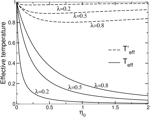
Figure 1: The effective stabilisation temperatures for each of the fields as a function of the viscosity coefficient $\eta_{0}$. The curves shown are for three values of $\lambda$ and $m=T=\eta_{c}=1$.

Equations (3) are represented graphically in Figure 1 for three different values of $\lambda$. Clearly, as $\eta_{0}$ increases from zero, $T_{\mathrm{eff}}$ decreases from the starting value $T$. The drop in temperature is more pronounced when the self coupling is smaller. $T_{\mathrm{eff}}$ approaches negligible values for $\eta_{0}\gtrsim\eta_{c}$ and sufficiently small $\lambda\lesssim 0.2$. This simply reflects that when the indirect interaction of $\phi_{0}$ with the heat bath is weaker this field dissipates its energy more efficiently. On the other hand, the field $\phi_{c}$ because of its direct coupling to the heat bath remains “hot”, i.e. $T^{\prime}_{\mathrm{eff}}$ stays close to $T$, but the larger $\lambda$ is, the more it deviates from $T$. This deviation is a natural consequence of the direct dissipative viscosity term for $\phi_{0}$ which is not balanced by any fluctuating effects. Although not shown in Figure 1 we have from (3) that when $\lambda\to\infty$ the effective temperatures become identical for any value of $\eta_{0}$.

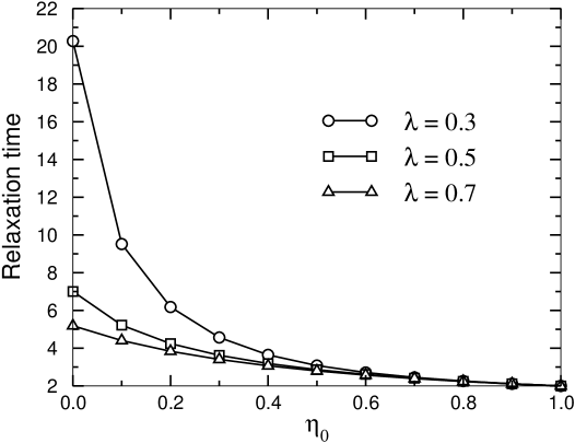
Figure 2: The relaxation times for $\phi_{0}$ as a function of the viscosity coefficient $\eta_{0}$. The curves are for three values of $\lambda$ and $m=T=\eta_{c}=1$.

The relaxation times for the decoupled fields for various values of the self-coupling are shown in Figure 2. The results were obtained by determining the eigenvalues of the homogeneous version of equations (3) (i.e. ignoring the noise term). The several relaxation time scales for the system are proportional to the inverse of the real part of these eigenvalues. In Figure 2 we show for each value of $\eta_{0}$ the largest of these time scales, which we interpret as the equilibration time for the uncoupled fields. We also checked that for all values of $\eta_{0}$ and $\lambda$ there is one eigenvalue leading to a relaxation time close to $2.0$, corresponding to the charged fields. When the two values of the dissipation are the same, for $\eta_{0}=\eta_{c}=1$, the two time scales coincide as expected. The rapid slowing down in the rate at which $\phi_{0}$ stabilises as $\lambda$ decreases shows a dependence closer to $\lambda^{-2}$ as we would expect. This naive expectation derives from the effective noise term ${\cal O}(\lambda)$ that the interacting potential induces in the equation for $\phi_{0}$ in the equations of motion (3).

In summary, by looking at a two field toy model we observe an unevenness in the way the kinetic energy is distributed between the “charged” and the “neutral” field. The conditions for this biasing are possible because of the presence of an external dissipation term and different strengths for the coupling of the fields to the heat bath. When the field with the weakest coupling to the bath is decoupled we recognise that this counterintuitive behaviour is due to a singularity in the limit of vanishing external dissipation. In a realistic situation the weakest coupling to the bath should not be neglected. The singular gives place to a two scale regime and the biasing is expect to occur when $\eta^{\mathrm{ext}}$ extracts energy at least at a rate comparable with the input from the bath coming from the weaker coupling. In the next section we will see how a similar effect contributes to a vacuum selection following a symmetry breaking phase transition.

4 Vacuum biasing in the $O(4)$ model

4.1 The use of the Langevin approach

We now return to the model described by the Lagrangean (1) and we will study its dynamical evolution under the Langevin approach already used in Sect. 3. In order to simulate the dynamics of the fields we use phenomenological Langevin equations

$$\Big{[}(\partial_{t}^{2}-\nabla^{2})-\mu^{2}+\lambda\sum_{k=1}^{4}\phi_{k}^{2}+\eta_{i}\partial_{t}\Big{]}\phi_{i}=\xi_{i},$$ (16)

with $\mu^{2}=\lambda v^{2}$, $v$ being the $T=0$ vacuum expectation value, and where $\eta_{i}$ and $\xi_{i}$ are respectively the viscosity coefficients and the Gaussian noises. For the fields that couple to the photon bath and that are assumed to thermalise at its temperature $T$, we have

$$\langle\xi_{i}(\vec{x},t)\xi_{j}(\vec{x}^{\prime},t^{\prime})\rangle=\Omega_{i}\delta_{ij}\delta^{(3)}(\vec{x}-\vec{x}^{\prime})\delta(t-t^{\prime}).$$ (17)

where $\beta\Omega_{i}=2\eta_{i}$, with $\beta=1/T$, according to the fluctuation-dissipation theorem. Below $T_{c}$ this relation is used only for $i=3,4$, while in the disordered phase it is assumed for all the fields.

In the ordered phase we consider the neutral fields to be decoupled from the bath, $\xi_{i}=0$, but let $\eta_{i}\neq 0$. The non vanishing value of these coefficients are due to an “external” source of dissipation. An expansion of the system, as in the early universe, is a possible origin for this type of dissipative term. In fact, this has been the main motivation behind this study. The toy model in the previous section showed us that even a small external dissipation could give rise to non negligible effects. In cosmology we expect a similar situation (except at very early times) in the sense that the dissipation due to the expansion of the universe is much smaller than the one associated to the charged fields which is due to the interactions with the “photon” bath.

It is in place to say something on the advantages and limitations of using the Langevin equations (16) at this stage. These equations describe the classical out-of-equilibrium evolution of a system of coupled fields. Therefore, at most, it provides effective equations for the long-wavelength modes of quantum fields with large occupation number. For this reason it is often used as a phenomenological set of equations to study close-to-equilibrium effects near phase transitions [10]. The use of the relativistic form of these type of equations has been motivated by cosmological applications [6, 7].

The relative simplicity of these equations is their main asset. We take the noise to be white and the dissipative kernel local both in space and time. Nevertheless, they provide a good starting set of equations to look for qualitative answers to questions in close-to-equilibrium dynamics provided one keeps a careful perspective of its shortcomings. This is the approach we take here.

The shortcomings of equations (16) are best understood when a more systematic derivation of the effective out-of-equilibrium dynamics from first principles is carried out [11, 12, 13]. The phenomenological approach to the study of hot non-Abelian plasmas provides also useful insights [14, 15]. There are, for instance, the questions on whether the origin of the noise is external or internal [13], or that the Langevin approach is only reliable near thermal equilibrium when a quasi-particle type of approximation can be justified. Let us say something briefly on the second issue.

One of the safest ways of understanding the regimes where a Langevin description applies in quantum field theory is to start from the Kadanoff-Baym equations [16] and work out under which conditions these equations can be interpreted as the result of Langevin processes [17]. The high temperature limit is a well established condition and is naturally implicit in (16) as this is an effective equation for long-wavelength modes, $k\ll T$. The use of classical equations is also justifiable by the more recent investigations on the reliability of the classical field theory limit to the dynamics of quantum fields out of equilibrium [18, 19, 8] at high $T$ or near $T_{c}$.

4.2 The simulations

We use a discretised version of (16) in three dimensional square lattices with $50^{3}$ to simulate the evolution of the $O(4)$ model (1). A leap-frog algorithm with time step $\delta_{t}=0.05$ is used. Larger lattices of $100^{3}$ have been used to verify the stability of our results. A Gaussian random number generator is used for the rapidly changing fluctuations. All quantities are measured in units of the $T=0$ vacuum expectation $v$. The dimensionless quantities are identified with a tilde. For example, $\widetilde{v}=1$ and $\widetilde{\beta}=v/T$. When choosing the lattice spacing we need to ensure that the modes with wavelength longer than $\sim T^{-1}$ are not cut off. In our runnings merely for reference we took physical scales from the chiral symmetry breaking effective mean field model. By using a lattice spacing $\widetilde{\Delta x}=0.25$ for $v=93$ MeV we can work up to temperatures of approximately $T\sim 350$ MeV.

We run our simulations for successive temperatures of the heat bath determined by $\Omega_{+}=2\eta_{+}T$, the amplitude for the noise of the charged scalars. Starting from a temperature $T>T_{c}$ we bring down the temperature across $T_{c}$. While in the disordered phase all the fields are taken to be in contact with the heat bath. It is only for $T<T_{c}$, when the vacuum expectation value starts to increase, that the neutral fields are decoupled.

In Figure 3, we plot the order parameters for the condensates of neutral and charged scalars against the inverse temperature $\beta$. These are, respectively, $\langle|\phi_{1}\phi_{2}|\rangle$ and $\langle|\phi_{3}\phi_{4}|\rangle$, where $\langle|\phi_{i}\phi_{j}|\rangle=\sqrt{\sum_{n=i,j}(\frac{1}{V}\int_{V}\phi_{n}(x))^{2}}$ are averages over the entire lattice. As the details of the decoupling of the neutral fields are not known we show the curves for three different types of decoupling. The label of instantaneous, exponential and power law refer to the way the variance $\Omega_{0}=\Omega_{0}(T)$ approaches zero starting from its value at the disordered phase as $T$ continues to decrease below $T_{c}$. For the runnings in Figure 3, the values of all the viscosity coefficients $\eta_{i}$ are kept the same for all the scalars. The different decouplings do not have an effect on the final values of the order parameters which always favour a non vanishing value for $\langle|\phi_{1}\phi_{2}|\rangle$. This shows a bias for the condensation of the neutral fields resulting from the relative large value of the ratio between the viscosity coefficient of the neutral by the charged scalar. Here we used $\eta_{0}/\eta_{+}=1$ to emphasise the case when the condensation of the neutral sector is strongly favoured.

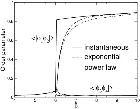
Figure 3: Diagram showing the variation in the order parameter as the system is cooled across $T_{c}$. We use $\lambda=1$ and a $50^{3}$ box. We show curves for three different decouplings: instantaneous, exponential and power law.

For the large value of $\eta_{0}$ used in the simulations for Figure 3 the neutral and the charged scalars have an equally effective channel to cool as the temperature decreases. However, the fluctuations coming from the interaction with the heat bath have the effect of slowing down the dissipation of the charged fields. This will favour the neutral fields to roll down more effectively to the bottom of the potential and condense.

The neutral fields are not blind to the photon bath due to the scalar self-coupling. They dissipate through the viscosity term but they gain energy via the scalar self-coupling. However, as long as the effects of fluctuations hitting the neutral modes is small and any increment of energy can quickly be dissipated, which occurs when $\lambda$ is not too large and $\eta_{0}$ not too small compared to $\eta_{+}$, the neutral scalars continue to monopolise the vacuum. As we discuss next the situation might change as $\eta_{0}$ decreases.

The curves in Figure 4, where we set $\eta_{0}=0$ but all other parameters are kept the same as in the runnings used for Figure 3, show that in this case the charged scalars condense. This suggests that as $\eta_{0}$ is decreased below some critical value the charged fields condense instead of the neutral ones. This results in a “superconducting” background where the photons are massive which clearly violates our working assumption of having a thermalised photon bath. Therefore, we conclude that the condensation of the charged scalars is an artifact of our simulations in this region of the parameter space of the model.

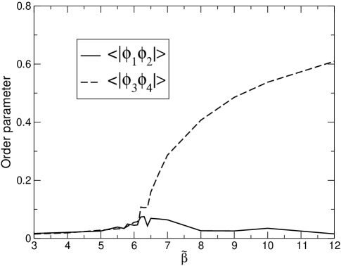
Figure 4: Diagram showing the vacuum selection favouring the charged scalars to condense when $\eta_{0}=0$ in the broken phase.

From the simulations we have discussed, we anticipate the existence of a critical value $\eta_{\mathrm{cr}}$ for $\eta=\eta_{0}/\eta_{+}$ in the interval $0<\eta_{\mathrm{cr}}<1$. A precise determination of $\eta_{\mathrm{cr}}$ is numerically delicate and at this phenomenological stage of our study it does not justify the dedicated effort it requires. For certain this critical value indicates the end of the validity of the context of our working conditions. This, we expect, indicates a qualitative change on the nature of the condensation.

The region of critical $\eta$ is characterised by competing domains of neutral and charged scalars, which might present analogies to disoriented chiral condensates [4]. In this region we have estimated the value of $\eta_{\mathrm{cr}}$ for varying self-coupling and present them in Table 1. Although the dependence with $\lambda$ is difficult to establish, our results give an indication that as $\lambda$ is increased by approximately one order of magnitude, $\lambda=4\to 20$, the critical value of $\eta$ also increases by a similar magnitude, $\eta_{\mathrm{cr}}\sim 10^{-5}\to 10^{-4}$. This is the behaviour we would naively expect from the fact that the scalar self-coupling is also a measure of the extent to which the decoupled fields have indirect contact with the photon bath. Finally, we remark that the results in the Table 1 for $\widetilde{\beta}=9$ might already fall outside the region where a classical description based on a Langevin approach is not reliable [8] as the system is no longer close to $T_{c}$.

Table 1: The table shows the values of $\langle|\phi_{1}\phi_{2}|\rangle$ and $\langle|\phi_{3}\phi_{4}|\rangle$. The three values of $\widetilde{\beta}$ correspond respectively to a temperature above, near and below $T_{c}$.

$\lambda=4$	$\widetilde{\beta}=4$		$\widetilde{\beta}=6$		$\widetilde{\beta}=9$
$\widetilde{\eta}_{0}=1\cdot 10^{-4}$	.011	.011	.113	.046	.607	.047
$\widetilde{\eta}_{0}=5\cdot 10^{-5}$	.011	.011	.072	.048	.586	.123
$\widetilde{\eta}_{0}=2\cdot 10^{-5}$	.011	.011	.057	.046	.552	.225
$\lambda=12$
$\widetilde{\eta}_{0}=2\cdot 10^{-4}$	.008	.008	.198	.089	.621	.126
$\widetilde{\eta}_{0}=1\cdot 10^{-4}$	.008	.008	.135	.157	.604	.185
$\widetilde{\eta}_{0}=5\cdot 10^{-5}$	.008	.008	.108	.165	.623	.111
$\lambda=20$
$\widetilde{\eta}_{0}=5\cdot 10^{-4}$	.007	.007	.292	.071	.649	.098
$\widetilde{\eta}_{0}=2\cdot 10^{-4}$	.007	.007	.133	.250	.639	.140
$\widetilde{\eta}_{0}=5\cdot 10^{-5}$	.007	.007	.074	.278	.650	.078

4.3 Interplay between parameters

It is useful to analyse the interplay between the various parameters in the model. To this end, we look at the kinetic energy of each set of fields, the coupled and the decoupled. Parallels with the toy model studied in the previous section will also be easier to draw. With this study we aim at learning how thermalisation is affected by the ratio of the viscosity coefficients $\eta=\eta_{0}/\eta_{+}$ and the scalar coupling $\lambda$.

In Figure 5 the time evolution of the kinetic energies for both types of scalar fields are plotted. The parameters $\widetilde{\eta}_{0}=0.005$, $\widetilde{\eta}_{+}=1$ and $\widetilde{\beta}=6.5$, all in units of the $T=0$ vacuum expectation value $v$ in a $100^{3}$ box, are the same for all the curves, whereas we use three different values for $\lambda$.

The equilibrium curve corresponds to the coupled fields which thermalise quickly in the time scales displayed in our plot. Of course “quickly” here means that the relaxation times for the decoupled fields are clearly longer than for the coupled ones. This occurs for all the parameter values shown. We verified that the temperature for the equilibrium curve is to a very good approximation consistent with the equipartition relation and therefore independent of $\lambda$. The external dissipation does not give origin to noticeable deviations from equipartition, as in the toy model, because of the present large number of degree of freedom.

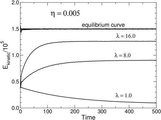
Figure 5: Diagram showing the kinetic energy of the scalar fields for a single value of $\eta=\eta_{0}/\eta_{c}$ and three different values of $\lambda$. For small values of $\lambda$ the neutral scalars approaches a steady state at a very slow rate.

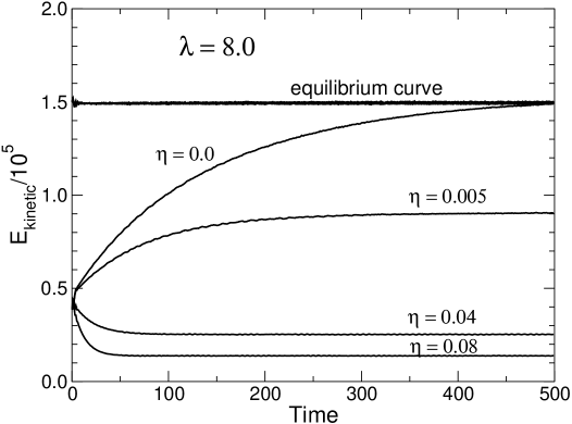
Figure 6: Diagram showing the kinetic energy of the scalar fields for a single value of $\lambda$ and four different values of $\eta=\eta_{0}/\eta_{c}$. The slowest relaxation time for the neutral fields occurs in the $\eta=0$ limit of no external dissipation.

The most interesting feature of Figure 5 is the $\lambda$ dependence of the asymptotic values for the kinetic energy of the decoupled fields. As in (3) we can interpret these quantities as effective equilibration temperatures $T_{\mathrm{eff}}$. We observe that the larger $\lambda$ is, the faster the decoupled fields approach a steady state. This is to be expected as the decoupled fields interact indirectly with the photon bath via the quartic scalar coupling. It explains not only the shorter relaxation times for larger values of $\lambda$ but also the higher $T_{\mathrm{eff}}$ values which get closer to the temperature of the bath.

We verified that the value of the asymptotic kinetic energies is independent of the initial conditions. In Figure 5 the starting kinetic energy of the decoupled fields is a third of the equipartition value. It is therefore safe to conclude that for weak scalar couplings the equilibrium state should be quite distinct from the equipartition thermalised state.

In Figure 6 we complement the curves shown in Figure 5 by keeping now the same scalar coupling for all the curves, here we use $\lambda=8$, and vary $\eta_{0}$, or equivalently $\eta$ as we again set $\eta_{+}=1$. We observe that the larger the viscosity coefficient $\eta_{0}$ the faster the decoupled fields equilibrate. On the other hand, as $\eta$ increases $T_{\mathrm{eff}}$ shifts away from $T$. The asymptotic steady state approaches the equilibrium curve only in the opposite limit, i.e. when the external dissipative channel is “switch off”. In this case, the kinetic energy does eventually reach the value expected by equipartition but at a clearly slow rate set by the magnitude of $\lambda$ via the fluctuations mediated by the scalar coupling.

4.4 Coupling the decoupled fields

We end this section with a discussion on the effects of introducing fluctuation terms to the evolution equations for the decoupled fields in analogy to what we have done in (13) for the toy model. The Langevin equations already include indirect interactions of the decoupled fields with the bath. However, one may still wonder if results might change when we include a more direct source of fluctuations. The most natural reason for introducing additional fluctuating forces is the interaction between the soft modes described by the Langevin equations and the associated scalar hard modes which should be present for both types of fields.

The relative strength of the different interactions is central here. Let $g$ denote the gauge coupling. Then our working assumption that the scalar self coupling is weak compared to the coupling to the photon bath means $g\gg\lambda$. In a simple perturbative estimate this implies that $\eta_{+}\gg\eta_{0}^{\mathrm{fl}}$. Qualitatively this relation is expected to hold at very high temperatures but more reliable non perturbative statements require more dedicated simulations.

In order for the external dissipation to have observable effects it can not be negligible with relation to both thermal dissipation coefficients. In our simulations this is trivially the case as $\eta_{+}\gg\eta_{0}^{\mathrm{ext}}=\eta_{0}^{\mathrm{}}$, but $\eta_{0}^{\mathrm{ext}}>\eta_{0}^{\mathrm{fl}}=0$. The first of these two inequalities justifies neglecting non thermal terms in the equations for the coupled scalars. In general, the biasing should occur as long as $\eta_{0}^{\mathrm{ext}}\gtrsim\eta_{0}^{\mathrm{fl}}\neq 0$. Let us see how our analysis supports this view.

Looking back at equation (15) we see that in the toy model the neutral field dissipation must be external for the effective temperatures of the asymptotic states to be different. A similar result applies to the $O(4)$ model where no vacuum selection occurs unless there is an external dissipation. From Figure 6 we recognise that it is necessary for the dissipation coefficient $\eta_{0}$ to have a non thermal external component. Clearly if $\eta_{0}$ had a purely thermal origin the kinetic energy of the neutral field would always asymptotically approach the equilibrium curve. This is expressed in the $\eta=0$ curve in Figure 6 as thermal dissipative effects are implicitly already present due to the scalar self-coupling. Adding an explicit coupling to a heat bath would only have the effect of decreasing the relaxation time.

5 Summary and discussion

In this paper we discussed the conditions that cause a selective condensation of neutral fields in an $O(4)$ symmetric scalar field sector of a field theory in three dimensions when this sector also includes charged fields. In particular, we studied a regime in the vicinity of a symmetry breaking transition where the interactions with a thermalised photon bath can be simulated by a phenomenological Langevin approach.

We show that under quite general conditions a non thermal dissipation in the evolution of the neutral fields effectively reduces the vacuum manifold of a system described by an $O(4)$ scalar model from $S^{3}$ to $S^{1}$, above a small dissipation threshold. From this analysis we identify the conditions that favour the formation and stabilisation of embedded defects as first argued by Nagasawa and Brandenberger [1].

The vacuum manifold reduction is due to the existence of different asymptotic steady states for the two types of scalar fields considered. This effect is caused by an “external” source of dissipation, in the sense that it does not arise from fluctuations resulting from interactions with the photon bath. The neutral field steady state is characterised by an effective temperature $T_{\mathrm{eff}}<T$, “colder” than the photon bath, and this is what leads to their selective condensation.

The remarkable feature is that even a small amount of “external” dissipation can be sufficient to cause qualitatively distinct effects, such as the vacuum selection. Small here is in relation to the dominant dissipation terms in the charged scalar field sector, which is related to the interaction with the photon bath by the fluctuation-dissipation theorem. This is counterintuitive. In principle, one would be inclined to neglect the possible effects of such a small amount of dissipation. For instance, the asymptotic state of the charged field sector is hardly affected by the “external” dissipation. What changes things is the existence of a small indirect thermal dissipation. Then the external dissipation needs at least to be of the order of the much smaller thermal dissipation coming from the indirect coupling of the neutral scalars with the heat bath.

We can naturally generalise the system to a more realistic one. First, the external dissipation is considered in both scalar field sectors. However, for the charged field sector this leads only to negligible corrections. Second, the neutral scalars are coupled directly to the heat bath although with a much weaker coupling than the charged scalars so that the resulting thermal dissipation for the former does not dominate over the non thermal external dissipation. Under these general conditions our results on vacuum selection are not qualitatively changed.

Finally, we note that possible corrections to the scalar fields potential coming from the interactions with the gauge bosons should not play an important role for our analysis. We know from the work of Nagasawa and Brandenberger [1] that the asymmetry created by the decoupling from the neutral fields from the photon bath biases the effective potential in a way that stabilises non topological defects when immersed in a photon plasma. Moreover, equilibrium thermal corrections to the potential tend to reduce the instability of these embedded configurations [21]. Therefore, at a perturbative level we do not expect corrections to counteract the vacuum selection we analyse here. A less investigated difficulty, but potentially an important one, is the contribution from very soft photons. Because of infra-red divergences reliable corrections similar to those in [11, 12] are not to our knowledge currently available. More dedicated simulations including the full dynamics of both the scalars and the gauge bosons are necessary to clarify this problem.

The type of scenario we describe here should be relevant for applications in the early universe where the expansion of the universe provides a non thermal source of dissipation. It would also be interesting to investigate if similar effects might take place in the quark-gluon plasma where different steady or intermediate states might coexist as in the bottom-up thermalisation in heavy-ion collision proposed in [20] driven by soft gauge bosons modes.

Acknowledgments

The authors would like to thank the referees for their constructive comments. It is a pleasure to acknowledge discussions with J. Berges, D. Panja, A. Patkos, J. Smit and A. Tranberg. F. F. would like to thank P. J. H. Denteneer and D. F. Litim for calling his attention to references [9] and [20] respectively. The work of F. F. was supported by FOM in the first part of this project, N. D. A. by PPARC and P. S. by the Magnus Ehrnrooth Foundation. This work is supported by the ESF Programme COSLAB - Laboratory Cosmology and the NWO under the VICI Programme.

References

- [1] M. Nagasawa and R. H. Brandenberger, Phys. Lett. B 467 (1999) 205 [hep-ph/9904261]; Phys. Rev. D 67 (2003) 043504 [hep-ph/0207246].
- [2] G. N. Felder, J. Garcia-Bellido, P. B. Greene, L. Kofman, A. D. Linde and I. Tkachev, Phys. Rev. Lett. 87 (2001) 011601 [hep-ph/0012142].
- [3] D. Boyanovsky and H. J. de Vega, Phys. Rev. D 47 (1993) 2343 [hep-th/9211044]; D. Boyanovsky, D. S. Lee and A. Singh, Phys. Rev. D 48 (1993) 800 [hep-th/9212083]; D. Boyanovsky, H. J. de Vega and R. Holman, Topological defects and the non-equilibrium dynamics of symmetry breaking phase transitions, Les Houches 1999, 139-169 [hep-ph/9903534].
- [4] A. A. Anselm, Phys. Lett. B 217 (1989) 169; J. D. Bjorken, Int. J. Mod. Phys. A 7 (1992) 4189; K. Rajagopal and F. Wilczek, Nucl. Phys. B 399 (1993) 395 [hep-ph/9210253]; Nucl. Phys. B 404 (1993) 577 [hep-ph/9303281].
- [5] Z. Xu and C. Greiner, Phys. Rev. D 62 (2000) 036012 [hep-ph/9910562].
- [6] M. Gleiser, Phys. Rev. Lett. 73 (1994) 3495 [hep-ph/9403310]; J. Borrill and M. Gleiser, Phys. Rev. D 51 (1995) 4111 [hep-ph/9410235].
- [7] N. D. Antunes, L. M. A. Bettencourt and M. Hindmarsh, Phys. Rev. Lett. 80 (1998) 908 [hep-ph/9708215].
- [8] R. J. Rivers and F. C. Lombardo, “How phase transitions induce classical behaviour”, hep-th/0412259.
- [9] Th. M. Nieuwenhuizen, Phys. Rev. Lett. 80 (1998) 5580; L. Cugliandolo and J. Kurchan, Physica A 263 (1999) 242.
- [10] N. Goldenfeld, “Lectures on phase transitions and the renormalization group”, Addison-Wesley (1992)
- [11] M. Gleiser and R. O. Ramos, Phys. Rev. D 50 (1994) 2441 [hep-ph/9311278]. A. Berera, M. Gleiser and R. O. Ramos, Phys. Rev. D 58 (1998) 123508 [hep-ph/9803394].
- [12] C. Greiner and B. Muller, Phys. Rev. D 55 (1997) 1026 [hep-th/9605048].
- [13] L. P. Csernai, S. Jeon and J. I. Kapusta, Phys. Rev. E 56, (1997) 6668 [nucl-th/9708033].
- [14] D. Bödeker, Phys. Lett. B 426 (1998) 351 [hep-ph/9801430]; Nucl. Phys. B 559 (1999) 502 [hep-ph/9905239].
- [15] D. F. Litim and C. Manuel, Phys. Rev. D 61 (2000) 125004 [hep-ph/9910348].
- [16] P. Danielewicz, Annals Phys. 152 (1984) 239; Annals Phys. 152 (1984) 305.
- [17] C. Greiner and S. Leupold, Annals Phys. 270 (1998) 328 [hep-ph/9802312]; Langevin interpretation of Kadanoff-Baym equations, hep-ph/9912229.
- [18] G. Aarts, G. F. Bonini and C. Wetterich, Nucl. Phys. B 587 (2000) 403 [hep-ph/0003262]; G. Aarts and J. Berges, Phys. Rev. Lett. 88 (2002) 041603 [hep-ph/0107129].
- [19] A. Arrizabalaga, J. Smit and A. Tranberg, JHEP 0410 (2004) 017 [hep-ph/0409177].
- [20] R. Baier, A. H. Mueller, D. Schiff and D. T. Son, Phys. Lett. B 502 (2001) 51 [hep-ph/0009237].
- [21] R. Holman, S. Hsu, T. Vachaspati and R. Watkins, Phys. Rev. D 46 (1992) 5352 [hep-ph/9208245].