Abstract

A structured mixed phase consisting of quark and hadron phases is numerically studied with the Coulomb screening effect and the surface effect. We carefully introduced the Coulomb potential, so that a geometrical structure becomes mechanically unstable when the surface tension is large. Charge densities are largely rearranged by the screening effect, and thereby the equation of state shows the similar behavior to that given by the Maxwell construction. Therefore, although bulk calculations with the Gibbs conditions show that the mixed phase may exist in a wide density region, we can see it is restricted to a narrow density region by the surface effect and the Coulomb screening effect.

1 Introduction

It has been believed that hadron matter changes to quark matter at high-density region by way of the “deconfinement phase transition”. Unfortunately the deconfinement phase transition have not been well understood up to now, and many authors have studied it by model calculations or by first-principle calculations like lattice QCD. These studies are now developing, and many exciting results have been reported. Properties of quark matter have been actively studied theoretically in quark-gluon plasma, color superconductivity [1, 2] or magnetism [3, 4, 5], and experimentally in relativistic heavy-ion collision (RHIC), HERA or early universe and compact stars [6, 7].

When we calculate uniform hadron matter (nuclear matter) and quark matter at zero temperature separately, by using the MIT bag model, we can expect the first-order phase transition as seen in Figs. 2 and 2. We can see that quark matter is an energetically favorable state at high-density region, $\rho>\rho_{\mathrm{c}}$ (Fig. 2). As we can see in Fig. 2, the thermodynamic potential of quark matter becomes lower at higher baryon-number chemical potential. These results suggest the deconfinement phase transition at high densities.

The features of the deconfinement phase transition have not been fully elucidated yet. We assume here that it is the first order phase transition, and use the bag model for simplicity. Then the thermodynamically forbidden region appears in the equation of state (EOS) and we can expect the mixed phase, the hadron-quark mixed phase, in some density region, which may exist in inner core region of neutron stars and during the hadronization of high-temperature quark-gluon plasma at RHIC experiment. We have to apply the Gibbs conditions (GC) to get EOS in thermodynamic equilibrium: GC demand chemical equilibrium, pressure valance and thermal equilibrium between two phases;

$$\mu_{\mathrm{B}}^{\mathrm{quark}}=\mu_{\mathrm{B}}^{\mathrm{hadron}}(\equiv\mu_{\mathrm{B}}),\hskip 5.0pt\mu_{\mathrm{Q}}^{\mathrm{quark}}=\mu_{\mathrm{Q}}^{\mathrm{hadron}}(\equiv\mu_{\mathrm{e}}),\hskip 5.0ptP^{\mathrm{quark}}=P^{\mathrm{hadron}},\hskip 5.0ptT^{\mathrm{quark}}=T^{\mathrm{hadron}},$$ (1)

where $\mu_{\mathrm{B}}^{i}$ and $\mu_{\mathrm{Q}}^{i}$ are baryon-number and charge chemical potentials, respectively. Thermal equilibrium is implicitly achieved at $T=0$. Note that there are two independent chemical potentials in this phase transition. In such a case the system should be much different from the liquid-vapor phase transition which is described by only one chemical potential.

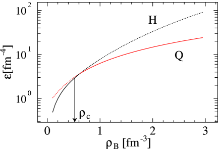
Figure 1: Energy density $\epsilon$ for uniform hadron matter and quark matter. Uniform quark matter is energetically favorable in high-density region, while hadron matter in low-density region.

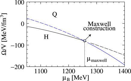
Figure 2: Thermodynamic potential $\Omega$ of uniform hadron matter and quark matter as a function of baryon chemical potential $\mu_{\mathrm{B}}$. Uniform quark matter is energetically favorable in high $\mu_{\mathrm{B}}$ region while hadron matter in low $\mu_{\mathrm{B}}$ region.

These GC must be fulfilled in the hadron-quark mixed phase. On the other hand, the Maxwell construction (MC) may be very familiar and has been used by many authors to get EOS for the first order phase transitions [8, 9, 10, 11]. It is well known that MC is a correct prescription to derive EOS for the liquid-vapor phase transition. However, Glendenning [12] pointed out that MC is not appropriate for the hadron-quark mixed phase: one of GC about the charge chemical equilibrium, $\mu_{\mathrm{Q}}^{\mathrm{quark}}=\mu_{\mathrm{Q}}^{\mathrm{hadron}}$, is not satisfied in MC, since the local charge neutrality is implicitly assumed without imposing this condition. He emphasized that the local charge neutrality is too restrictive and each hadron or quark phase may have a net charge because only the total charge must be kept neutral.

When we use GC in the bulk calculation, which we explain in detail later, we can see the mixed phase appears in a large density region. The pressure is not constant as density changes in the mixed phase, while only a constant pressure is obtained from MC as shown in Refs. [12, 13].

However, the bulk calculation is too simple and Heiselberg et al. [14] claimed the importance of including the finite-size effects, i.e., the surface tension at the hadron-quark boundary and the Coulomb interaction energy. They studied the quark droplet immersed in hadron matter and found that it is energetically unfavorable if the surface tension is large enough. On the contrary, however, if the surface tension is not large the mixed phase can exist in some density region.

Glendenning and Pei [15] suggested the crystalline structure by a bulk calculation using the small surface tension: one phase is immersed in another phase with various geometrical structures; “droplet”, “rod”, “slab”, “tube”, and “bubble”. These are called the structured mixed phases (SMP). Applying the results based on the bulk calculation to neutron stars, they suggested that there could develop SMP in the core region for several kilo meters in thickness.

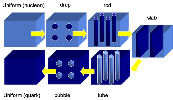
Figure 3: Schematic view of the structured mixed phases.

At a first glance, this view seems to be reasonable and there may appear the mixed phase in a large density region. However, there are still many points to be elucidated about the finite-size effects. Voskresensky et al. emphasized that the proper treatment of the Coulomb interaction is important in the mixed phase [16].

First note that there is the relation between chemical potential and the Coulomb potential by way of the gauge transformation: chemical potential is not well defined before the gauge fixing. Secondly, the charge chemical equilibrium could be rather satisfied even in MC, once the Coulomb potential $V_{\mathrm{Coul}}$ is incorporated:

$$\hfill\mu_{\mathrm{Q}}^{\mathrm{quark}}\ =\mu_{\mathrm{Q}}^{\mathrm{hadron}},$$ (2)

whereas

$$\mu_{\mathrm{Q}}^{\mathrm{quark}}-V_{\mathrm{Coul}}^{\mathrm{quark}}\neq\mu_{\mathrm{Q}}^{\mathrm{hadron}}-V_{\mathrm{Coul}}^{\mathrm{hadron}}.$$ (3)

Note that the electron chemical potential $\mu_{e}=\mu_{Q}$ and the electron number density can be expressed in terms of the combination, $\left(\mu_{\mathrm{Q}}-V_{\mathrm{Coul}}\right)$ (see Eq. (48)), when the Coulomb potential $V_{\rm Coul}$ is introduced. Therefore, Eqs. (2), (3) mean that the charge chemical potential is equal, while the electron number is different between the hadron and quark phases. Equation (3) is reduced to $\mu_{e}^{\rm quark}\neq\mu_{e}^{\rm hadron}$ in the absence of the Coulomb potential, which is the previous claim that the charge chemical equilibrium is apparently violated in MC. Thus we can see that the previous claim means nothing but the difference of the electron number in two phases [16]. Thirdly, it is important to take into account the Coulomb screening effect. We have to solve the Poisson equation consistently with other equations of motion for charged particles. Actually, Voskresensky et al.  showed SMP is mechanically unstable by the Coulomb screening effect when the surface tension is not small. If SMP is mechanically unstable, the phase transition should be similar to that in MC.

It can be easily seen that there should occur rearrangement of charged particle densities by the Coulomb interaction. On the contrary such rearrangement modifies the Coulomb potential. As a result the Poisson equation becomes highly non-linear and difficult to solve analytically. In their study, a linear approximation (RPA) was employed to solve the Poisson equation analytically. It is valid to use the approximation for pointing out the important property of SMP, but it may be conceivable that various charge properties like “global charge neutrality” for GC, “local charge neutrality” for MC, and “the Coulomb screening effect” have important roles in the mixed phase. Therefore, solving the Poisson equation without any approximation is of much significance. We have reported a preliminary result for the case of droplet [18]. It would be also very interesting to derive EOS in our consistent calculation for the hadron-quark matter phase transition.

2 Bulk calculation with the Gibbs conditions

Now we consider two infinite matters separated by a sharp boundary: uniform quark matter and hadron matter. We consider the quark phase consists of u, d, s quarks and electron, and the hadron phase proton, neutron and electron. We discard the Coulomb interaction in the calculation. Then we can evaluate the total thermodynamic potential $\Omega_{\mathrm{tot}}$:

$$\Omega_{\mathrm{tot}}=\Omega_{\mathrm{u}}+\Omega_{\mathrm{d}}+\Omega_{\mathrm{s}}+\Omega_{\mathrm{n}}+\Omega_{\mathrm{p}}+\Omega_{\mathrm{e}}.$$ (4)

The explicit expressions of $\Omega_{i}$ for non-uniform matter are given in the next section. We use them by replacing the space dependent quantities by constants for each uniform matter.

Introducing the volume fraction of the quark phase $f$, we impose the global charge neutrality: the total charge density vanishes,

$$f\rho_{\mathrm{Q}}+(1-f)\rho_{\mathrm{H}}=0,$$ (5)

where $\rho_{\mathrm{Q}}$ and $\rho_{\mathrm{H}}$ are the net charge densities of the quark and hadron phases, respectively,

$$\begin{split}\rho_{\mathrm{Q}}&=\frac{2}{3}\rho_{\mathrm{u}}-\frac{1}{3}\rho_{\mathrm{d}}-\frac{1}{3}\rho_{\mathrm{s}}-\rho_{\mathrm{e}},\\ \rho_{\mathrm{H}}&=\rho_{\mathrm{p}}-\rho_{\mathrm{e}}.\end{split}$$ (6)

Note that we have now six chemical potentials; $\mu_{\mathrm{u}}$, $\mu_{\mathrm{d}}$, $\mu_{\mathrm{s}}$, $\mu_{\mathrm{p}}$, $\mu_{\mathrm{n}}(\equiv\mu_{\mathrm{B}})$, $\mu_{\mathrm{e}}$. We first consider $\beta$ equilibrium in each phase and chemical equilibrium at the hadron-quark boundary. Thus all chemical potentials are constant. The chemical equilibrium conditions then are:

$$\mu_{\mathrm{u}}+\mu_{\mathrm{e}}=\mu_{\mathrm{d}},$$ (7)

$$\mu_{\mathrm{d}}=\mu_{\mathrm{s}},$$ (8)

in the quark phase,

$$\mu_{\mathrm{p}}+\mu_{\mathrm{e}}=\mu_{\mathrm{n}}$$ (9)

in the hadron phase, and

$$\mu_{\mathrm{n}}=\mu_{\mathrm{u}}+2\mu_{\mathrm{d}},$$ (10)

$$\mu_{\mathrm{p}}=2\mu_{\mathrm{u}}+\mu_{\mathrm{d}},$$ (11)

at the hadron-quark interface. The last condition (11) can be derived from other four conditions, so that there are left four independent conditions for chemical equilibrium. Therefore, if we give two chemical potentials $\mu_{\mathrm{B}}$ and $\mu_{\mathrm{e}}$ by hand, we can determine these four chemical potentials; $\mu_{\mathrm{u}}$, $\mu_{\mathrm{d}}$, $\mu_{\mathrm{s}}$ and $\mu_{\mathrm{p}}$ from these four equations.

Next, we can determine $\mu_{\mathrm{e}}$ by the global charge neutrality condition (5). $f$ is still unknown at this point and finally, we find the optimal value of $f$ by using one of GC; $P^{\mathrm{quark}}=P^{\mathrm{hadron}}$, where pressure $P$ is given by the thermodynamic relation: $P=-\Omega/V$. Thus once $\mu_{\mathrm{B}}$ is given, all other values $\mu_{i}$ ($i=u,d,s,p,e$) and $f$ can be obtained.

We show the results of the bulk calculation. We present the charge densities in Fig. 4. We can see the total charge density is zero, while the quark phase is negatively charged and the hadron phase positively charged. Note that MC always gives a null charge density in each phase due to the local charge neutrality [13].

Figure 4: Charge density of each phase. The total charge density is always zero.

Figure 6 shows pressure versus baryon-number density. The most important difference between “Maxwell” and “Bulk Gibbs” is that the pressure given by MC is constant while that given by the bulk calculation with GC is density dependent. Remember that the outstanding feature in these two results comes from that each hadron or quark phase has a net charge in “Bulk Gibbs”, while each phase is neutral in “Maxwell”.

The phase diagram in the $\mu_{\rm B}-\mu_{\rm e}$ plane is presented in Fig. 6. We can easily see that the charge chemical potential $\mu_{\mathrm{e}}$ is much different between uniform hadron matter and quark matter for MC, which means chemical equilibrium condition for $\mu_{\mathrm{e}}$ is not satisfied in MC. Thus it could be said that MC is not a proper way in the bulk calculation. Glendenning [12] pointed out this defect in MC and showed another result (Bulk Gibbs) within the bulk calculation. One can easily see that the mixed phase appears in a wide $\mu_{\mathrm{B}}$ region in Fig. 6.

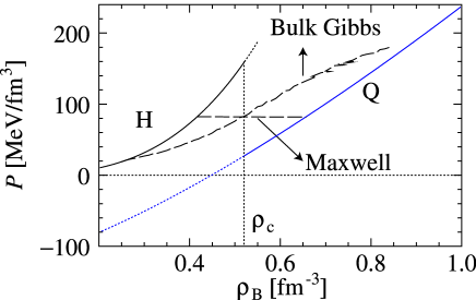
Figure 5: Pressure of uniform matter, that given by the bulk calculation with GC (Bulk Gibbs) and that given by MC (Maxwell).

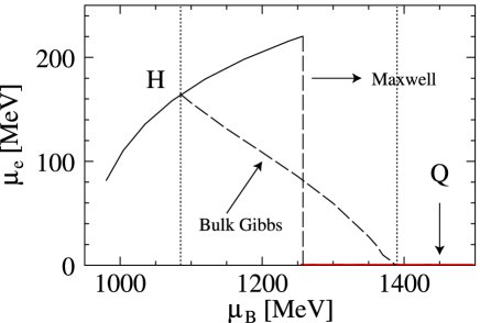
Figure 6: Phase diagram in the chemical potential plane. H means uniform hadron matter and Q uniform quark matter. Other notations have the same meaning as in Fig. 6

After the claim by Glendenning, Heiselberg et al. [14] demonstrated that the finite-size effects may disfavor the mixed phase by extending the bulk calculation to include the Coulomb interaction and the surface energy. On the other hand, Glendenning and Pei [15] suggested “crystalline structures of the mixed phase” because SMP are energetically more favorable than uniform matter even including the surface and Coulomb effects.

Voskresensky et al. pointed out the importance of the Coulomb screening effect and suggested the usefulness of MC for the mixed phase. We have seen MC is apparently incorrect because if we apply MC to this mixed phase, one of GC, charge chemical equilibrium, is violated. However, once the Coulomb interaction is taken into account, there is still a room to satisfy the condition without spoiling the picture given by MC, as noted in the previous section. Since the Coulomb screening effect had been taken into account with an approximation in their study, we may still address a question, “is the picture derived from MC is completely meaningless when we include the Coulomb interaction in a proper way?”. All we have to do next is to solve the Poisson equation without any approximation, strictly satisfying GC.

3 Formalism

3.1 Density Functional Theory

We use the idea of the Density Functional Theory (DFT) [19, 20] to study the quark-hadron mixed phase. We employ here the Thomas-Fermi approximation, which gives the simple expressions for the energies. We summarize below some energy expressions with the local density approximation (LDA); the expressions are first derived for uniform system, and then we regard densities as the space-dependent functions.

First, the kinetic energy is simply expressed as

$$\epsilon(\rho(\bm{r})) = \frac{2}{\left(2\pi\right)^{3}}\int_{0}^{p_{\mathrm{F}}(\bm{r})}d^{3}p\sqrt{p^{2}+m^{2}}$$

$$= \frac{m^{4}}{8\pi^{2}}\left[\frac{p_{\mathrm{F}}(\bm{r})}{m}\sqrt{1+\left(\frac{p_{\mathrm{F}}(\bm{r})}{m}\right)^{2}}\left(2\left(\frac{p_{\mathrm{F}}(\bm{r})}{m}\right)^{2}+1\right)\right.$$

$$\left.\hskip 56.9055pt-\ln\left(\frac{p_{\mathrm{F}}(\bm{r})}{m}+\sqrt{1+\left(\frac{p_{\mathrm{F}}(\bm{r})}{m}\right)^{2}}\right)\right],$$

where $m$ is the particle mass and the Fermi momentum $p_{\mathrm{F}}(\bm{r})$ is expressed by the density profile $\rho(\bm{r})$ as $p_{\mathrm{F}}(\bm{r})=\left(\pi^{2}\rho(\bm{r})\right)^{\frac{1}{3}}$.

Next, we consider the interaction energy of quarks. We take the first-order contribution which comes from the one-gluon exchange interaction in uniform quark matter,

$$\begin{tabular}[]{c}\includegraphics[width=85.35826pt,height=85.35826pt,keepaspectratio]{oge.eps2}\end{tabular}=\overline{\psi}(p_{2})\left(-ig\gamma_{\mu}\frac{\lambda_{a}}{2}\right)\psi(p_{1})D^{\mu\nu}(p^{\prime})\overline{\psi}(p_{4})\left(-ig\gamma_{\nu}\frac{\lambda_{a}}{2}\right)\psi(p_{3}).$$ (13)

Here $\lambda_{a}$ is the SU(3) Gell-Mann matrix and $D^{\mu\nu}$ the gluon propagator [21]. By way of the Wick contraction, the Hartree and Fock terms are derived:

$$\mathop{\vbox{\halign{#\cr\kern 1.72218pt\cr$\hbox{$\hskip 6.94446pt\vrule height=7.31946pt,width=0.29999pt,depth=-0.66708pt\kern-0.29999pt\vrule height=7.31946pt,width=53.16515pt,depth=-7.01947pt\kern-0.29999pt\vrule height=7.31946pt,width=0.29999pt,depth=-0.11153pt$\hss}\hbox{$\hskip 110.38705pt\vrule height=7.31946pt,width=0.29999pt,depth=-0.66708pt\kern-0.29999pt\vrule height=7.31946pt,width=53.25511pt,depth=-7.01947pt\kern-0.29999pt\vrule height=7.31946pt,width=0.29999pt,depth=-0.11153pt$\hss}$\crcr\kern 1.72218pt\nointerlineskip\cr\hbox{$\displaystyle{\overline{\psi}}{(}{q)\left(-ig\gamma_{\mu}\frac{\lambda_{a}}{2}\right)}{\psi}{(q)D^{\mu\nu}(0)\overline{\psi}}{(}{k)\left(-ig\gamma_{\nu}\frac{\lambda_{a}}{2}\right)}{\psi}(k)$}\crcr}}}\limits=\begin{tabular}[]{c}\includegraphics[width=85.35826pt,height=85.35826pt,keepaspectratio]{hartree.eps2}\end{tabular}$$ (14)

for the Hartree term, and

$$\mathop{\vbox{\halign{#\cr\kern 1.72218pt\cr$\hbox{$\hskip 6.94446pt\vrule height=10.97919pt,width=0.29999pt,depth=-0.66708pt\kern-0.29999pt\vrule height=10.97919pt,width=170.51704pt,depth=-10.6792pt\kern-0.29999pt\vrule height=10.97919pt,width=0.29999pt,depth=-0.11153pt$\hss}\hbox{$\hskip 60.1096pt\vrule height=7.31946pt,width=0.29999pt,depth=-0.11153pt\kern-0.29999pt\vrule height=7.31946pt,width=64.09679pt,depth=-7.01947pt\kern-0.29999pt\vrule height=7.31946pt,width=0.29999pt,depth=-0.66708pt$\hss}$\crcr\kern 1.72218pt\nointerlineskip\cr\hbox{$\displaystyle{\overline{\psi}}{(}{q)\left(-ig\gamma_{\mu}\frac{\lambda_{a}}{2}\right)}{\psi}{(k)D^{\mu\nu}(q-k)\overline{\psi}}{(}{k)\left(-ig\gamma_{\nu}\frac{\lambda_{a}}{2}\right)}{\psi}(q)$}\crcr}}}\limits=\begin{tabular}[]{c}\includegraphics[width=85.35826pt,height=85.35826pt,keepaspectratio]{fock.eps2}\end{tabular}$$ (15)

for the Fock term. Due to the traceless property of $\lambda_{a}$, ${\rm Tr}\lambda_{a}=0$, the Hartree term gives a null contribution in the color-singlet quark matter,

$$\mathop{\vbox{\halign{#\cr\kern 1.72218pt\cr$\hbox{$\hskip 6.94446pt\vrule height=7.31946pt,width=0.29999pt,depth=-0.66708pt\kern-0.29999pt\vrule height=7.31946pt,width=53.25511pt,depth=-7.01947pt\kern-0.29999pt\vrule height=7.31946pt,width=0.29999pt,depth=-0.11153pt$\hss}$\crcr\kern 1.72218pt\nointerlineskip\cr\hbox{$\displaystyle{\overline{\psi}}{(}{k)\left(-ig\gamma_{\nu}\frac{\lambda_{a}}{2}\right)}{\psi}(k)$}\crcr}}}\limits=\mathrm{Tr}\left[\overline{\psi}\psi\left(-ig\gamma_{\nu}\frac{\lambda_{a}}{2}\right)\right]=0.$$ (16)

Therefore only the Fock term contributes to the interaction energy, which becomes

$$\begin{tabular}[]{c}\includegraphics[width=71.13188pt,height=71.13188pt,keepaspectratio]{fock2.eps2}\end{tabular}=-\frac{1}{8}g^{2}\mathrm{Tr}\left(\lambda_{a}\lambda_{a}\right)\int\!\!\!\int\frac{d^{4}k}{\left(2\pi\right)^{4}}\frac{d^{4}q}{\left(2\pi\right)^{4}}\mathrm{Tr}\left(\gamma_{\mu}G_{D}(q)\gamma_{\nu}G_{D}(k)\right)D^{\mu\nu}(q-k)$$ (18)

$$=-64\alpha_{s}\pi\int\!\!\!\int\frac{d^{3}q}{(2\pi)^{3}}\frac{d^{3}k}{(2\pi)^{3}}n_{q}n_{k}\frac{1}{4k^{0}q^{0}}\left(2m_{f}^{2}-kq\right)\frac{-1}{\left(k-q\right)^{2}}\equiv\epsilon_{\mathrm{Fock}}.$$ (19)

Here $G_{D}$ is the density-dependent quark propagator [21]. The subscript $f$ denotes the flavor, $m_{f}$ the quark mass, $k^{0}=\left(|\bm{k}|^{2}+m_{f}^{2}\right)^{1/2}$ and $n_{k}=\theta(k_{\mathrm{F}f}-|\bm{k}|)$ with the Fermi momentum $k_{\mathrm{F}f}$. After some manipulation we easily find

$$\epsilon_{\mathrm{Fock}}=-\frac{\alpha_{s}}{\pi^{3}}\sum_{\mathrm{f}}m_{f}^{4}\left\{x_{{f}}^{4}-\frac{3}{2}\left[x_{{f}}\eta_{{f}}-\ln\left(x_{{f}}+\eta_{{f}}\right)\right]^{2}\right\},$$ (20)

where $\displaystyle x_{f}=\frac{p_{\mathrm{F}f}(\bm{r})}{m_{f}}$ and $\eta_{f}=\sqrt{1+x_{f}^{2}}$, and we use the relation $p_{\mathrm{Ff}}(\bm{r})=\left(\pi^{2}\rho_{f}(\bm{r})\right)^{\frac{1}{3}}$. Equation (20) becomes $\epsilon_{\rm Fock}=\frac{1}{2}\frac{\alpha_{s}}{\pi^{3}}\sum_{f}p_{Ff}^{4}$ for massless particles.

For the interaction energy of nucleons, we use for simplicity the effective potential parametrized by densities [16],

$$\epsilon_{\mathrm{pot}}(\bm{r}) = S_{0}\frac{\left(\rho_{\mathrm{n}}(\bm{r})-\rho_{\mathrm{p}}(\bm{r})\right)}{\rho_{0}(\bm{r})}+\left(\rho_{\mathrm{n}}(\bm{r})+\rho_{\mathrm{p}}(\bm{r})\right)\epsilon_{\mathrm{bind}}$$ (21)

$$+K_{0}\frac{\left(\rho_{\mathrm{n}}(\bm{r})+\rho_{\mathrm{p}}(\bm{r})\right)}{18}\left(\frac{\rho_{\mathrm{n}}(\bm{r})+\rho_{\mathrm{p}}}{\rho_{0}(\bm{r})}-1\right)^{2}$$

$$+C_{\mathrm{sat}}\left(\rho_{\mathrm{n}}(\bm{r})+\rho_{\mathrm{p}}(\bm{r})\right)\left(\frac{\rho_{\mathrm{n}}(\bm{r})+\rho_{\mathrm{p}}(\bm{r})}{\rho_{0}}-1\right),$$

where, $S_{0}$, $K_{0}$, $\epsilon_{\mathrm{bind}}$, and $C_{\mathrm{sat}}$ are adjustable parameters to satisfy the saturation properties of nuclear matter.

3.2 Thermodynamic potential

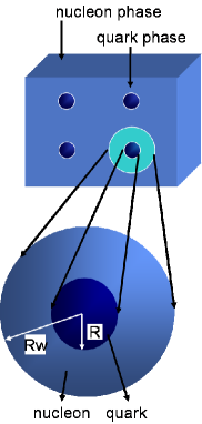
Figure 7: Wigner-Seitz approximation.

We consider a system which consists of the hadron and quark phases. We divide the whole space into equivalent and charge-neutral Wigner-Seitz cells with the size $R_{W}$ and the droplet size $R$ as illustrated in Fig. 7. Here we only consider the droplet phase. Following DFT we begin with the thermodynamic potential in terms of particle density profiles and chemical potentials, $\mu_{i}^{\mathrm{Q}}$ and $\mu_{i}^{\mathrm{H}}$,

$$\Omega_{\mathrm{tot}}=E(\rho_{i}(\bm{r}))-\sum_{i}\mu_{i}^{\mathrm{Q}}\int_{0}^{R}\!\!d\bm{r}\,\rho_{i}^{\mathrm{Q}}(\bm{r})-\sum_{i}\mu_{i}^{\mathrm{H}}\int_{R}^{R_{W}}\!\!d\bm{r}\,\rho_{i}^{\mathrm{H}}(\bm{r}).$$ (22)

To take into account the Coulomb interaction, we write it in terms of the $i$-particle density profiles; $\rho_{i}(\bm{r})$ with $Q_{i}$ being the particle charge ($Q=-e<0$ for the electron),

$$V_{\mathrm{Coul}}(r)=-\sum_{i}\int d^{3}r^{\prime}\frac{Q_{i}\rho_{i}(\bm{r}^{\prime})}{\left|\bm{r}-\bm{r}^{\prime}\right|}.$$ (23)

Applying the Laplacian $\nabla^{2}$ on Eq. (23), we can easily derive the Poisson equation $\nabla^{2}V_{\mathrm{Coul}}=4\pi e^{2}\sum_{i}Q_{i}\rho_{i}(\bm{r})$. The Coulomb interaction energy $E_{V}$ is then expressed as

$$E_{V}=\frac{1}{2}\sum_{i,j}\int d^{3}rd^{3}r^{\prime}\frac{Q_{i}\rho_{i}(\bm{r})Q_{j}\rho_{j}(\bm{r}^{\prime})}{\left|\bm{r}-\bm{r}^{\prime}\right|}.$$ (24)

Including the surface term, the total energy is expressed as

$$E(\rho_{i}(\bm{r}))=\int_{0}^{R}d\bm{r}\epsilon_{\mathrm{Q}}+\int_{R}^{R_{W}}d\bm{r}\epsilon_{\mathrm{H}}+\int_{S}dS\epsilon_{S}+E_{V},$$ (25)

where $\epsilon_{S}$ means the surface-energy density, $S$ boundary area, and $\epsilon_{\mathrm{Q}}$ and $\epsilon_{\mathrm{H}}$ the energy densities in the quark and hadron phases. Since we poorly know the details of the hadron quark interface, we simply approximate the surface energy as $\displaystyle\int_{S}dS\epsilon_{S}\equiv\sigma S$ by using the surface tension $\sigma$. Each chemical potential is derived by the equation of motion $\displaystyle\frac{\delta\Omega_{\mathrm{tot}}}{\delta\rho_{i}(\bm{r})}=0$, which reads $\displaystyle\mu_{i}=\frac{\delta E(\rho_{i}(\bm{r}))}{\delta\rho_{i}(\bm{r})}$, or

$$\mu_{i} = \frac{\delta E_{\mathrm{kin+str}}}{\delta\rho_{i}(\bm{r})}-N_{i}V(\bm{r}),\hskip 10.0ptN_{i}=\frac{Q_{i}}{e},$$ (26)

$$E_{\mathrm{kin+str}} = \int_{0}^{R}d\bm{r}\epsilon_{\mathrm{Q}}+\int_{R}^{R_{W}}d\bm{r}\epsilon_{\mathrm{H}}.$$ (27)

As we have seen in the previous section, each phase may have a finite net charge. In the previous studies of SMP, the Coulomb interaction between charged particles has been treated rather simply: the Coulomb energy was added to the total energy by using the volume fraction $f$ and constant densities derived for two infinite matters [14, 22]. Thus the Coulomb screening effect and rearrangement of charge densities are completely discarded. One important point we would like to address here is, when there is the Coulomb interaction, the gauge variance of chemical potentials should be taken into account. Differentiating the expression of chemical potential (26) with respect to the Coulomb potential $V(\bm{r})$, we get the relation [16],

$$A_{ij}\frac{\partial\rho_{j}}{\partial V} = N_{i},$$ (28)

$$A_{ij}B_{jk} = \delta_{ik},$$ (29)

where matrices $A$ and $B$ are defined as

$$A_{ij}\equiv\frac{\delta^{2}E_{\mathrm{kin+str}}}{\delta\rho_{i}\delta\rho_{j}},\ \ \ B_{ij}\equiv\frac{\partial\rho_{i}}{\partial\mu_{j}}.$$ (30)

From these equations, the gauge invariance relation is derived,

$$\frac{\partial\rho_{i}}{\partial V}=N_{j}\frac{\partial\rho_{j}}{\partial\mu_{i}}.$$ (31)

We can immediately see that the chemical potential is gauge variant from this equation: when the Coulomb potential is shifted by a constant value, $V(\bm{r})\Longrightarrow V({\bm{r}})-V_{0}$, the chemical potential should also be shifted $\mu_{i}\Longrightarrow\mu_{i}+N_{i}V_{0}$ to keep the gauge invariance. Note that the charge density should be observable and gauge invariant; we shall see the constant shift of the Coulomb potential is compensated by the redefinition of the chemical potential in the expression of the charge density. The Poisson equation is also gauge invariant because it is not changed by the constant shift of the Coulomb potential. Therefore, if the Poisson equation is not properly taken into account, the gauge invariance is obviously violated.

Next, we present the explicit form of the thermodynamic potential for each particle. First, we consider the quark phase which consists of u, d and s quarks and electron. According to the small current quark mass, we treat u and d quarks as massless particles and only s quark massive (150 MeV) in this phase. Electron is also treated as a massless particle. Next, we consider hadron phase which consists of proton, neutron and electron. Nucleons are treated as non-relativistic particles. The total thermodynamic potential becomes

$$\Omega_{\mathrm{tot}}=\Omega_{\mathrm{Q}}+\Omega_{\mathrm{H}}+E_{S}.$$ (32)

Here $\Omega_{\rm Q}$ and $\Omega_{\rm H}$ are the thermodynamic potentials in the quark and hadron phases, and $E_{S}$ the surface energy.

3.2.1 Quark phase (u, d, s quarks)

The thermodynamic potentials in the quark phase are given by Eqs. (3.1), (20), (25):

$$\Omega_{\mathrm{Q}} = \Omega_{\mathrm{u}}+\Omega_{\mathrm{d}}+\Omega_{\mathrm{s}}+\Omega_{\mathrm{em}}^{\mathrm{Q}}+\int_{0}^{R}d\bm{r}B\hskip 10.0pt\hbox{($B$ : bag constant)}.$$ (33)

$$\Omega_{\mathrm{u}} = \int_{0}^{R}d^{3}r\left[\frac{3\pi^{\frac{2}{3}}}{4}\left(1+\frac{2\alpha_{s}}{3\pi}\right)\rho_{\mathrm{u}}^{\frac{4}{3}}(\bm{r})-\mu_{\mathrm{u}}\rho_{\mathrm{u}}(\bm{r})-\frac{2}{3}V_{\mathrm{Coul}}(\bm{r})\rho_{\mathrm{u}}(\bm{r})\right],$$ (34)

$$\Omega_{\mathrm{d}} = \int_{0}^{R}d^{3}r\left[\frac{3\pi^{\frac{2}{3}}}{4}\left(1+\frac{2\alpha_{s}}{3\pi}\right)\rho_{\mathrm{d}}^{\frac{4}{3}}(\bm{r})-\mu_{\mathrm{d}}\rho_{\mathrm{d}}(\bm{r})+\frac{1}{3}V_{\mathrm{Coul}}(\bm{r})\rho_{\mathrm{d}}(\bm{r})\right],$$ (35)

$$\Omega_{\mathrm{s}} = \int_{0}^{R}d^{3}r\left[\epsilon_{\mathrm{s}}(\rho_{\mathrm{s}}(\bm{r}))-\mu_{\mathrm{s}}\rho_{\mathrm{s}}(\bm{r})+\frac{1}{3}V_{\mathrm{Coul}}(\bm{r})\rho_{\mathrm{s}}(\bm{r})\right],$$ (36)

$$\Omega_{\mathrm{em}}^{\mathrm{Q}} = \int_{0}^{R}d^{3}r\left[-\frac{1}{8\pi e^{2}}\left(\nabla V_{\mathrm{Coul}}(\bm{r})\right)^{2}+\frac{\left(3\pi^{2}\rho_{e}(\bm{r})\right)^{\frac{4}{3}}}{4\pi^{2}}-\mu_{e}\rho_{e}(\bm{r})+V_{\mathrm{Coul}}(\bm{r})\rho_{e}(\bm{r})\right].$$ (37)

Here, $\Omega_{\mathrm{em}}^{\mathrm{Q}}$ summarizes the electron and another Coulomb contributions. The energy density of s quark $\epsilon_{\mathrm{s}}(\rho_{\mathrm{s}}(\bm{r}))$ is a function of $\rho_{\mathrm{s}}(\bm{r})$, which is explicitly expressed by using Eqs. (3.1) and (20) as

$$\epsilon_{\mathrm{s}}(\rho_{\mathrm{s}}(\bm{r}))=\left\{\frac{3m_{\mathrm{s}}^{4}}{8\pi^{2}}\left[\frac{p_{\mathrm{Fs}}(\bm{r})}{m_{\mathrm{s}}}\sqrt{1+\left(\frac{p_{\mathrm{Fs}}(\bm{r})}{m_{\mathrm{s}}}\right)^{2}}\left(2\left(\frac{p_{\mathrm{Fs}}(\bm{r})}{m_{\mathrm{s}}}\right)^{2}+1\right)\right.\right.$$

$$\left.\left.-\ln\left(\frac{p_{\mathrm{Fs}}(\bm{r})}{m_{\mathrm{s}}}+\sqrt{1+\left(\frac{p_{\mathrm{Fs}}(\bm{r})}{m_{\mathrm{s}}}\right)^{2}}\right)\right]-\frac{\alpha_{s}}{\pi^{3}}\left[p_{\mathrm{Fs}}^{4}(\bm{r})-\frac{3}{2}m_{\mathrm{s}}^{4}\left[\frac{p_{\mathrm{Fs}}(\bm{r})}{m_{\mathrm{s}}}\sqrt{1+\left(\frac{p_{\mathrm{Fs}}(\bm{r})}{m_{\mathrm{s}}}\right)^{2}}\right.\right.\right.$$

$$\left.\left.\left.-\ln\left(\frac{p_{\mathrm{Fs}}(\bm{r})}{m_{\mathrm{s}}}+\sqrt{1+\left(\frac{p_{\mathrm{Fs}}(\bm{r})}{m_{\mathrm{s}}}\right)^{2}}\right)\right]^{2}\right]\right\}.$$ (38)

3.2.2 Hadron phase (non-relativistic nucleons)

The thermodynamic potentials in the hadron phase read,

$$\Omega_{\mathrm{H}} = \Omega_{\mathrm{n}}+\Omega_{\mathrm{p}}+\Omega_{\mathrm{em}}^{\mathrm{H}}+\int_{R}^{R_{\mathrm{W}}}d\bm{r}\epsilon_{\mathrm{pot}}(\bm{r})\hskip 10.0pt\hbox{here $\epsilon_{\mathrm{pot}}(\bm{r})$ is Eq.\ (\ref{effpot}).}$$ (39)

$$\Omega_{\mathrm{n}} = \int_{R}^{R_{W}}d^{3}r\left[\frac{3}{10m}\left(3\pi^{2}\right)^{\frac{2}{3}}\rho^{\frac{5}{3}}_{\mathrm{n}}(\bm{r})-\mu_{\mathrm{n}}\left(\rho_{\mathrm{p}}(\bm{r}),\rho_{\mathrm{n}}(\bm{r})\right)\rho_{\mathrm{n}}(\bm{r})\right],$$ (40)

$$\Omega_{\mathrm{p}} = \int_{R}^{R_{W}}d^{3}r\left[\frac{3}{10m}\left(3\pi^{2}\right)^{\frac{2}{3}}\rho^{\frac{5}{3}}_{\mathrm{p}}(\bm{r})-\mu_{\mathrm{p}}\left(\rho_{\mathrm{p}}(\bm{r}),\rho_{\mathrm{n}}(\bm{r})\right)\rho_{\mathrm{p}}(\bm{r})-V_{\mathrm{Coul}}(\bm{r})\rho_{\mathrm{p}}(\bm{r})\right],$$ (41)

$$\Omega_{\mathrm{em}}^{\mathrm{H}} = \int_{R}^{R_{W}}d^{3}r\left[-\frac{1}{8\pi e^{2}}\left(\nabla V_{\mathrm{Coul}}(\bm{r})\right)^{2}+\frac{\left(3\pi^{2}\rho_{e}(\bm{r})\right)^{\frac{4}{3}}}{4\pi^{2}}-\mu_{e}\rho_{e}(\bm{r})+V_{\mathrm{Coul}}(\bm{r})\rho_{e}(\bm{r})\right].$$ (42)

Here $\Omega_{\mathrm{em}}^{\mathrm{H}}$ summarizes the electron and another Coulomb contributions.

3.3 Equations of motion

We get the expression of chemical potentials and the Poisson equation from the equation of motion $\frac{\partial\Omega}{\partial\phi_{i}}=0$, where $\phi_{i}=\rho_{u}(\bm{r}),\rho_{d}(\bm{r}),\rho_{s}(\bm{r}),\rho_{p}(\bm{r}),\rho_{n}(\bm{r}),\rho_{e}(\bm{r}),V_{\mathrm{Coul}}(\bm{r})$. The Poisson equation is explicitly written as

$$\nabla^{2}V_{\mathrm{Coul}}(\bm{r})=4\pi e^{2}\left[\left(\frac{2}{3}\rho_{u}(\bm{r})-\frac{1}{3}\rho_{d}(\bm{r})-\frac{1}{3}\rho_{s}(\bm{r})\right)\theta(R-r)+\rho_{\mathrm{p}}(\bm{r})\theta(r-R)-\rho_{e}(\bm{r})\right].$$ (43)

The chemical potentials for quarks in the quark phase are derived as

$$\mu_{\mathrm{u}} = \left(1+\frac{2\alpha_{s}}{3\pi}\right)\pi^{\frac{2}{3}}\rho_{\mathrm{u}}^{\frac{1}{3}}(\bm{r})-\frac{2}{3}V_{\mathrm{Coul}}(\bm{r}),$$ (44)

$$\mu_{\mathrm{d}} = \left(1+\frac{2\alpha_{s}}{3\pi}\right)\pi^{\frac{2}{3}}\rho_{\mathrm{d}}^{\frac{1}{3}}(\bm{r})+\frac{1}{3}V_{\mathrm{Coul}}(\bm{r}),$$ (45)

$$\mu_{\mathrm{s}} = \epsilon_{{\mathrm{Fs}}}+\frac{2\alpha_{s}}{3\pi}\left[p_{\mathrm{Fs}}(\bm{r})-3\frac{m_{\mathrm{s}}^{2}}{\epsilon_{\mathrm{Fs}}}\ln\left(\frac{\epsilon_{\mathrm{Fs}}+p_{\mathrm{Fs}}(\bm{r})}{m_{\mathrm{s}}}\right)\right]+\frac{1}{3}V_{\mathrm{Coul}}(\bm{r}).$$ (46)

Here, we use $\epsilon_{\mathrm{Fs}}=\sqrt{m_{\mathrm{s}}^{2}+p_{\mathrm{Fs}}^{2}}$ and $p_{\mathrm{Fs}}=(\pi^{2}\rho_{\mathrm{s}}(\bm{r}))^{\frac{1}{3}}$. The nucleon chemical potentials in the hadron phase and the electron chemical potential are

$$\mu_{\mathrm{n}} = \frac{p_{\mathrm{Fn}}^{2}}{2m}+\frac{2S_{0}\left(\rho_{n}(\bm{r})-\rho_{\mathrm{p}}(\bm{r})\right)}{\rho_{0}}+\epsilon_{\mathrm{bind}}+\frac{K_{0}}{6}\left(\frac{\rho_{\mathrm{n}}(\bm{r})+\rho_{\mathrm{p}}(\bm{r})}{\rho_{0}}-1\right)^{2}$$ (48)

$$+\frac{K_{0}}{9}\left(\frac{\rho_{\mathrm{n}}(\bm{r})+\rho_{\mathrm{p}}(\bm{r})}{\rho_{0}}-1\right)+2C_{\mathrm{sat}}\frac{\rho_{\mathrm{n}}(\bm{r})+\rho_{\mathrm{p}}(\bm{r})}{\rho_{0}}-C_{\mathrm{sat}},$$

$$\mu_{\mathrm{p}} = \mu_{\mathrm{n}}-\frac{p_{\mathrm{Fn}}^{2}}{2m}+\frac{p_{\mathrm{Fp}}^{2}}{2m}-\frac{4S_{0}\left(\rho_{\mathrm{B}}(\bm{r})-2\rho_{\mathrm{p}}(\bm{r})\right)^{2}}{\rho_{0}}-V_{\mathrm{Coul}}(\bm{r}),$$ (49)

$$\mu_{e} = \left(3\pi^{2}\rho_{e}(\bm{r})\right)^{\frac{1}{3}}+V_{\mathrm{Coul}}(\bm{r}).$$ (50)

Note that, e.g., the electron density profile $\rho_{\mathrm{e}}(\bm{r})$ is expressed as

$$\rho_{\mathrm{e}}(\bm{r})=\frac{\left(\mu_{\mathrm{e}}-V_{\mathrm{Coul}}(\bm{r})\right)^{3}}{3\pi^{2}},$$ (51)

in a gauge invariant fashion (cf. Eq. (3)). We impose the $\beta$ equilibrium in the quark and hadron phases and the chemical equilibrium at the quark-hadron boundary as in Eqs. (7)-(11). The pressure contribution from the surface tension is derived as $P_{\sigma}=\sigma\frac{dS}{dV_{\mathrm{Q}}}$ with $V_{\mathrm{Q}}$ being the volume of the quark droplet. From Eqs. (33) and (39), the pressure of each phase is expressed as

$$P^{\mathrm{Q}}=-\frac{\Omega_{\mathrm{Q}}}{V_{\mathrm{Q}}},\hskip 5.0ptP^{\mathrm{H}}=-\frac{\Omega_{\mathrm{H}}}{V_{\mathrm{H}}},$$ (52)

with $V_{\mathrm{H}}$ being the volume of hadron phase. Therefore the pressure balance condition becomes

$$P^{\mathrm{Q}}=P^{\mathrm{H}}+P_{\sigma},$$ (53)

which gives the droplet size $R$. Finally the cell size $R_{W}$ is determined by the minimum condition for $\Omega_{\mathrm{tot}}$. Particle density profiles and $R$, $R_{W}$ are completely determined for given $\mu_{\mathrm{B}}$. Thus we can solve these coupled equations of motion consistently with GC. Note that the Coulomb potential is included in a proper way and $V_{\mathrm{Coul}}(\bm{r})$ appears in almost all chemical potentials. The Coulomb potential is a functional of the charged-particle density profiles and in turn densities are functions of the Coulomb potential. As a result, the Poisson equation becomes highly non-linear. Since it is difficult to solve analytically, we solve it numerically without any approximation, whereas the linear approximation has been used in the previous work [16].

4 Numerical results

We show a case of quark droplet embedded in hadron matter for the volume fraction $f=(R/R_{\mathrm{W}})^{3}=1/100$ and the surface tension $\sigma=60$ MeV/fm². We can see the Coulomb screening effect in Fig. 8. There is always a minimum in the thermodynamic potential with respect to the droplet radius $R$ without the Coulomb screening, due to the balance between the Coulomb energy and the surface energy. However, once the Coulomb screening is taken into account, the minimum disappears, which shows the mechanical instability caused by the Coulomb screening effect. If the surface tension is large enough, the geometrical structure (droplet) becomes mechanically unstable by the Coulomb screening.

Next, we show the density profiles. We can see the flat density profile of particles in the left panel of Fig. 9, where there is no Coulomb screening effect. In the right panel, on the other hand, we can see the rearrangement of the charged particles as the Coulomb screening effect.

Let us consider the features of these density profiles in detail. In the quark phase, the densities of the negatively charged d, s quarks and electron are reduced, while that of the positively charged u quarks are enhanced by the Coulomb screening effect. Remember that the quark phase has a negative charge and the hadron phase a positive charge in the hadron-quark mixed phase.

Figure 8: Radial dependence of the thermodynamic potential $\Omega$ for the droplet structure. Solid and dashed lines are $\Omega$ with and without screening, respectively.

For the hadron phase, we can see the opposite effect by the Coulomb screening: the electron number increases and the proton number is reduced. We see that the charged particles in one phase are also affected by the charge of another phase: negatively charged particles in the quark phase are attracted to the surface, while positively charged particles (u quarks) are repelled from the surface. On the contrary, the positively charged particles in the hadron phase (protons) are attracted to the surface, while electrons are repelled. Although the rearrangement effect is not enough to establish the local charge neutrality, we can understand that the Coulomb screening effect is to reduce the local charge in each phase.

To draw the phase diagram of the hadron-quark mixed phase, we have to minimize the thermodynamic potential with respect to the volume fraction, i.e., we have to change the droplet radius $R$ and Wigner-Seitz cell size $R_{\mathrm{w}}$.

Figure 9: Density profiles $\rho_{i}$ without the Coulomb screening effect (left panel) and with the Coulomb screening effect (right panel). This is the case of $\mu_{\mathrm{B}}=1232$ MeV and the volume fraction $f=\left(R/R_{\mathrm{W}}\right)^{3}=0.01$. Each density uniformly spreads in each phase and $V_{\mathrm{Coul}}$ is constant ( =0 ) in the left panel, while there is rearrangement of the charge densities and $V_{\mathrm{Coul}}$ is spatially dependent in the right panel.

We show the total thermodynamic potential for the droplet phase in Fig. 10. Comparing with uniform hadron matter and quark matter, the droplet phase takes the smallest value of thermodynamic potential between a certain range of the baryon-number chemical potential. To clarify the difference between uniform matter and the droplet phase, we show the difference of thermodynamic potential between them in the right panel of Fig. 10.

We can see a large difference between our result ($\sigma=40$ MeV/fm²) and that given by the bulk calculation in Fig. 10.

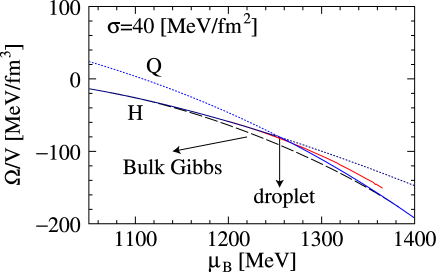
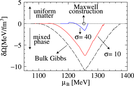
Figure 10: Thermodynamic potential $\Omega$ (left panel) and its difference from uniform hadron matter and quark matter $\delta\Omega$ (right panel). The dashed line “Bulk Gibbs”, in the right panel, shows the difference between the bulk calculation and uniform matter. Solid lines are the cases for the droplet phase with $\sigma=10$ and 40 MeV/fm².

If the difference $\delta\Omega$ is negative, the mixed phase is an energetically favorable state. On the contrary, if $\delta\Omega$ is positive, the mixed phase is an unfavorable state. In the right panel of Fig. 10, the point given by the Maxwell construction is specified by a circle ($\mu_{\mathrm{B}}\sim 1257$ MeV, $\delta\Omega=0$), where the following relations are maintained,

$$\mu_{\mathrm{B}}^{\mathrm{quark}}=\mu_{\mathrm{B}}^{\mathrm{hadron}}(\equiv\mu_{\mathrm{B}}),\hskip 5.0ptP^{\mathrm{quark}}=P^{\mathrm{hadron}},\hskip 5.0ptT^{\mathrm{quark}}=T^{\mathrm{hadron}}.$$ (54)

Note that if we naively apply MC, we have to discard one of GC, $\mu_{\mathrm{e}}^{\mathrm{quark}}=\mu_{\mathrm{e}}^{\mathrm{hadron}}$ in the absence of the Coulomb potential. The curve of “Bulk Gibbs” shows that the mixed phase is energetically favorable in the wide $\mu_{\mathrm{B}}$ region, as is already seen in Sec. 2. The difference $\delta\Omega$ for “Bulk Gibbs” is up to 10 MeV/fm³, while for the droplet phase ($\sigma=40$ MeV/fm²), it is only less than 2 MeV/fm³. This shows that if we use the larger value of the surface tension, the mixed phase gets more unfavorable. This feature is similar to that reported by Heiselberg [14] or Alford [22]. We can see the region of the energetically favorable mixed phase in the right panel of Fig. 10: the region becomes narrower than “Bulk Gibbs”, which means that the property of the mixed phase is closer to that given by MC. Thus we have seen that the mixed phase is very much affected by the Coulomb screening effect and the surface effect, by strictly keeping GC. For the larger value of the surface tension, MC is effectively useful in the description of the hadron-quark mixed phase. Note that we never violate the condition for the charge chemical equilibrium $\mu_{\mathrm{e}}^{\mathrm{hadron}}=\mu_{\mathrm{e}}^{\mathrm{quark}}$ to get these conclusions. Remember that the meaning of the condition in the presence of the Coulomb potential is different from that in the absence of the Coulomb potential.

5 Summary and concluding remarks

In this note we have first seen how the bulk calculation is performed for the hadron-quark mixed phase by applying the Gibbs conditions to the system consisting of two infinite matters. It gives a wide density region for the mixed phase. Based on this result, some authors also suggested the structured mixed phase with various geometrical structures, by including the finite-size effects, the surface and Coulomb energies [14, 22].

We have examined the finite-size effects in the mixed phase by numerically solving the equations of motion for the particle densities and the Poisson equation for the Coulomb potential. Our framework is based on the idea of the density functional theory, which, we believe, is one of the best theories to treat the structured mixed phases. We have demonstrated, by taking the droplet phase as an example, that the Coulomb screening effect and rearrangement of the charge densities play an important role for the mechanical instability as well as the energy of the mixed phase. As a result we have seen that the region of the mixed phase is highly restricted by the Coulomb screening effect as well as the surface energy. We have also seen that EOS gives the similar behavior to that given by the Maxwell construction, whereas the Maxwell construction is apparently incorrect in a system with more than one chemical potential: the Maxwell construction is effectively useful in the description of the mixed phase, even in this case. As another case of more than one chemical potential, kaon condensation has been also studied [23] and the result is similar to the present case.

We have included the surface tension, but its definite value is not clear and many authors treated it as a free parameter. There are also many estimations for the surface tension at the hadron-quark interface in lattice QCD [24, 25], in shell-model calculations [26, 27, 28] and in model calculations based on the Dual-Ginzburg Landau theory [29]. If we have the realistic value of the surface tension, we can reasonably bring out SMP in the hadron-quark phase transition. As these system corresponds to neutron star matter, we have seen that the mixed phase should be narrow by the finite-size effects. Our result would restrict the allowed SMP region in neutron stars which is suggested by Glendenning [15, 13]. It could be said that they should change the property of neutron stars especially in equation of state [30].

We have assumed in relation to phenomenological implications here that temperature is zero. It would be much interesting to include the finite-temperature effect. Then it is possible to draw the phase diagram in the $\mu_{\mathrm{B}}-T$ plane and we can study the properties of the deconfinement phase transition. In this study we have used a simple model for quark matter to figure out the finite-size effects in the structured mixed phase. However, it has been suggested that the color superconductivity is a ground state of quark matter [1, 22]. To get more realistic picture of the hadron-quark phase transition, we will need to take into account color superconductivity. In the recent studies the mixed phase has been also studied [31, 32].

References

- [1] M. Alford, K. Rajagopal and F. Wilczek, Nucl. Phys. B 64 (1999) 443, D. Bailin and A. Love, Phys. Rep. 107 (1984) 325. As resent reviews, M. Alford, hep-ph/0102047; K. Rajagopal and F. Wilczek, hep-ph/0011333, D. H. Rischke, Prog. Part. Nucl. Phys. 52 (2004) 197
- [2] M. Alford and S. Reddy, Phys. Rev. D 67 (2003) 074024
- [3] T. Tatsumi, T. Maruyama and E. Nakano, Prog. Theor. Phys. Suppl. 153 (2004) 190
- [4] E. Nakano, T. Maruyama and T. Tatsumi, Phys. Rev. D 68 (2003) 105001
- [5] T. Tatsumi, Phys. Lett. B 489 (2000) 280
- [6] J. Madsen, Lect. Notes Phys. 516 (1999) 162
- [7] K. S. Cheng, Z. G. Dai and T. Lu, Int. Mod. Phys. D7 (1998) 139
- [8] W. Weise, and G. E. Brown, Phys. lett. B 58 (1975) 300
- [9] A. B. Migdal, A. I. Chernoustan and I. N. Mishustin, Phys. lett. B 83 (1979) 158
- [10] J. Ellis, J. Kapusta and K. A. Olive, Nucl. Phys. B 348 (1991) 345
- [11] A. Rosenhauer, E. F. Staubo, L. P. Csernai, T. Øvergård, and E. Østgaad, Nucl. Phys. A 540 (1992) 630
- [12] N. K. Glendenning, Phys. Rev. D D46 (1992) 1274; Phys. Rep. 342 (2001) 393.
- [13] N. K. Glendenning, Compact stars, Springer 2000.
- [14] H. Heiselberg, C. J. Pethick and E. F. Staubo, Phys. Rev. Lett. 70 (1993) 1355
- [15] N. K. Glendenning and S. Pei, Phys. Rev. C D52 (1995) 2250
- [16] D. N. Voskresensky, M. Yasuhira and T. Tatsumi, Phys. Lett. B541 (2002) 93; Nucl. Phys. A723 (2003) 291; T. Tatsumi, M. Yasuhira and D. N. Voskresensky, Nucl. Phys. A718 (2003) 359c; T. Tatsumi and D. N. Voskresensky, nucl-th/0312114.
- [17] T. Norsen and S. Reddy, Phys. Rev. C. 63 (2001) 065804
- [18] T. Endo, Toshiki Maruyama, S. Chiba and T. Tatsumi, Nucl. Phys. A 749 (2005) 333
- [19] R. G. Parr and W. Yang, Density-Functional Theory of atoms and molecules, Oxford Univ. Press, 1989.
- [20] E. K. U. Gross and R. M. Dreizler, Density functional theory, Plenum Press (1995)
- [21] R. Tamagaki and T. Tatsumi, Prog. Theor. Phys. Suppl. 112 (1993) 277
- [22] M. Alford, K. Rajagopal, S. Reddy, and F. Wilczek, Phys. Rev. D 64 (2001) 074017
- [23] Toshiki Maruyama, T. Tatsumi, D. N. Voskresensky, T. Tanigawa and S. Chiba, Nucl. Phys. A 749 (2005) 186
- [24] K. Kajantie, L. Kärkäinen, and K. Rummukainen, Nucl. Phys. B357 (1991) 693
- [25] S. Huang, J. Potvion, C. Rebbi and S. Sanielevici, Phys. Rev. D 43 (1991) 2056
- [26] J. Madsen, Phys. Rev. D 46 (1992) 329
- [27] J. Madsen, Phys. Rev. Lett. 70 (1993) 391
- [28] M. S. Berger and R. L. Jaffe, Phys. Rev. C 35 (1987) 213
- [29] H. Monden, H. Ichie, H. Suganuma and H. Toki, Phys. Rev. C 57 (1998) 2564
- [30] T. Endo, Toshiki Maruyama, S. Chiba and T. Tatsumi, in preparation.
- [31] I. Shovkovy, M. Hanauske and M. Huang, Phys. Rev. D 67 (2003) 103004
- [32] S. Reddy and G. Rupak, nucl-th/0405054