Pair Production of Charged Higgs Bosons from Bottom-Quark Fusion

Abstract

For very large values of $\tan\beta$, the charged Higgs boson pair production via $b\bar{b}$ annihilation can proceed dominantly at the Large Hadron Collider (LHC) . We calculated the cross sections of the charged Higgs boson pair production via subprocess $b\bar{b}\to H^{+}H^{-}$ at the LHC including the next-to-leading order (NLO) QCD corrections in the minimal supersymmetric standard model (MSSM). We find that the NLO QCD corrections can significantly reduce the dependence of the cross sections on the renormalization and factorization scales.

PACS: 14.80. Cp, 12.60.Jv, 12.38.Bx

I. Introduction

One of the most important missions of future high-energy experiments is to search for scalar Higgs bosons and explore the electroweak symmetry breaking mechanism. In the standard model (SM)[1], one doublet of complex scalar fields is needed to spontaneously break the symmetry, leading to a single neutral Higgs boson $h^{0}$. The minimal supersymmetric standard model (MSSM) [2] is one of the most attractive extensions of the SM. The MSSM requires the existence of two doublets of Higgs fields to cancel anomalies and to give masses separately to up and down-type fermions. The MSSM predicts two CP-even neutral Higgs bosons $h^{0},H^{0}$, a pseudoscalar $A^{0}$ Higgs boson and a pair of charged scalar particles $H^{\pm}$. At the tree level, the MSSM Higgs sector has two free parameters: $\tan\beta=v_{2}/v_{1}$, the ratio of the vacuum expectation values of the two Higgs doublets and a Higgs boson mass which is taken to be $m_{H^{\pm}}$ in this paper.

The discovery of the $H^{\pm}$ would be a clear signal for the existence of physics beyond the SM with a strong hint towards supersymmetry. The CERN large hadron collider (LHC), with $\sqrt{s}=14~{}TeV$ and a luminosity of 100 ${\rm fb}^{-1}$ per year, will be a wonderful tool for looking for new physics. At the LHC, the light charged Higgs boson can be produced from the top quark decays $t\to b+H^{+}$[3]. Heavy charged Higgs boson is mainly produced via the processes $g\bar{b}\to\bar{t}H^{+}$[4], $gg\to\bar{t}bH^{+}$[5] and $qb\to q^{\prime}bH^{+}$[6]. Moreover, single charged Higgs boson production associated with a $W$ boson, via tree-level $b\bar{b}$ annihilation and one-loop $gg$ fusion, has been proposed and analyzed in Ref.[7].

At the LHC, the charged Higgs boson also can be produced in pair production mode. There are three important $H^{+}H^{-}$ production channels: (i) $q\bar{q}\to H^{+}H^{-}$, where $q=u,d,c,s,b$. (via Drell-Yan process, where a photon and a Z-boson are exchanged in the $s$-channel. In the case of $q=b$, there are additional Feynman diagrams involving $h^{0}$ and $H^{0}$ in the $s$-channel and the top quark in the $t$-channel) [8]. For very large values of $\tan\beta$, due to the large contributions from the additional diagrams, the $H^{+}H^{-}$ production can proceed dominantly via $b\bar{b}$ annihilation [9]. (ii) $gg\to H^{+}H^{-}$ (via quarks and squarks loop) [9][10] . (iii) $qq\to qqH^{+}H^{-}$ (via vector boson fusion) [11].

In the subprocess $b\bar{b}\to H^{+}H^{-}$, the initial state bottom quarks arise from a gluon in the proton splitting into a collinear $b\bar{b}$-pair, parameterized in terms of bottom quark distribution functions. On the other hand, the ’twin’ process $gg\to b\bar{b}H^{+}H^{-}$ using gluon density has been studied at LO in Ref.[12]. It is pointed out that the use of the b-quark density may overestimate the inclusive cross section due to crude approximations in the kinematics [13]. However, it is suggested that the bottom quark parton approximation maybe valid by choosing appropriate factorization scale [14]. Following the suggestions in Ref.[13, 14], we can analyze the transverse momentum distribution of the b-quarks in the process $gg\to b\bar{b}H^{+}H^{-}$ as shown in Fig.2 of Ref.[12]. The most suitable factorization scale for $b\bar{b}\to H^{+}H^{-}$ is of order $m_{H^{\pm}}/5\sim m_{H^{\pm}}/4$ which is much smaller than the usually used scale $m_{H^{\pm}}$.

In this paper, we study the process $pp\to b\bar{b}\to H^{+}H^{-}+X$ at the LHC with very large $\tan\beta$ in the MSSM. The NLO QCD corrections are calculated. The paper is organized as follow: In section 2, we discuss the LO results of the subprocess $b\bar{b}\to H^{+}H^{-}$. In section 3, we present the calculations of the NLO QCD corrections. In section 4, the numerical results, discussions and conclusions are presented.

II. The Leading Order Cross Section

The Feynman diagrams for the subprocess $b(p_{1})\bar{b}(p_{2})\to H^{+}(k_{3})H^{-}(k_{4})$ at the LO are shown in Fig.1, where $p_{1,2}$ and $k_{3,4}$ represent the four-momenta of the incoming partons and the outgoing particles respectively.

Figure 1: The tree level Feynman diagrams for $b\bar{b}\to H^{+}H^{-}$.

We divide the tree-level amplitude into two parts,

$$M^{0}=M_{0}^{(s)}+M_{0}^{(t)},$$ (2.1)

where $M_{0}^{(s)}$ and $M_{0}^{(t)}$ represent the amplitudes arising from the s-channel diagrams shown in Fig.1(a,b,c,d) and the t-channel diagram shown in Fig.1(e) respectively. The explicit expressions for the amplitudes $M_{0}^{(s)}$ and $M_{0}^{(t)}$ can be written as

$$M_{0}^{(t)} = i\bar{v}(p_{2})\frac{(P_{R}g^{(1)}_{H^{+}tb}+P_{L}g^{(2)}_{H^{+}tb})(m_{t}+\hbox to0.0pt{/\hss}p_{1}-\hbox to0.0pt{/\hss}k_{3})(P_{L}g^{(1)}_{H^{+}tb}+P_{R}g^{(2)}_{H^{+}tb})}{\hat{t}-m^{2}_{t}}u(p_{1}),$$

$$M_{0}^{(s)} = i\bar{v}(p_{2})[\frac{g_{H^{+}H^{-}h^{0}}g_{h^{0}b\bar{b}}}{\hat{s}-m^{2}_{h^{0}}}+\frac{g_{H^{+}H^{-}H^{0}}g_{H^{0}b\bar{b}}}{\hat{s}-m^{2}_{H^{0}}}-\frac{Q_{b}e^{2}(\hbox to0.0pt{/\hss}k_{3}-\hbox to0.0pt{/\hss}k_{4})}{\hat{s}}$$ (2.2)

$$- \frac{(c^{2}_{w}-s^{2}_{w})e^{2}}{2c^{2}_{w}s^{2}_{w}}\frac{(\hbox to0.0pt{/\hss}k_{3}-\hbox to0.0pt{/\hss}k_{4})(s^{2}_{w}/3-P_{L}/2)}{\hat{s}-m^{2}_{Z}}]u(p_{1}),$$

where $\hat{s}=(p_{1}+p_{2})^{2}$, $\hat{t}=(p_{1}-k_{3})^{2}$ and $\hat{u}=(p_{1}-k_{4})^{2}$ are the usual Mandelstam variables. $P_{L,R}=(1\mp\gamma_{5})/2$, $s_{w}=\sin\theta_{w}$, $c_{w}=\cos\theta_{w}$,$Q_{b}=-1/3$. The couplings are defined below,

$$g^{(1)}_{H^{+}tb} = \frac{iem_{t}}{\sqrt{2}m_{W}s_{w}\tan\beta},~{}~{}~{}~{}~{}~{}g^{(2)}_{H^{+}tb}=\frac{ie\overline{m}_{b}(\mu_{r})\tan\beta}{\sqrt{2}m_{W}s_{w}},$$

$$g_{h^{0}b\bar{b}} = \frac{ie\overline{m}_{b}(\mu_{r})}{2m_{W}s_{w}}\frac{\sin\alpha}{\cos\beta},~{}~{}~{}~{}~{}~{}g_{H^{0}b\bar{b}}=-\frac{ie\overline{m}_{b}(\mu_{r})}{2m_{W}s_{w}}\frac{\cos\alpha}{\cos\beta},$$

$$g_{H^{+}H^{-}h^{0}} = -\frac{iem_{W}}{s_{w}}(\sin(\beta-\alpha)+\frac{\cos(2\beta)\sin(\alpha+\beta)}{2c^{2}_{w}}),$$

$$g_{H^{+}H^{-}H^{0}} = -\frac{iem_{W}}{s_{w}}(\cos(\beta-\alpha)-\frac{\cos(2\beta)\cos(\alpha+\beta)}{2c^{2}_{w}}),$$ (2.3)

where $\alpha$ is the mixing angle which leads to the physical Higgs eigenstates $h^{0}$ and $H^{0}$. $\overline{m}_{b}(\mu_{r})$ is $\overline{\rm MS}$ running mass of the bottom quark. We neglected the bottom quark mass during our calculation except in the Yukawa couplings.

Then the LO cross section for the subprocess $b\bar{b}\to H^{+}H^{-}$ is obtained by using the following formula:

$$\hat{\sigma}^{0}(\hat{s},b\bar{b}\to H^{+}H^{-})=\frac{1}{16\pi\hat{s}^{2}}\int_{\hat{t}_{min}}^{\hat{t}_{max}}d\hat{t}~{}\overline{\sum}|M^{0}|^{2},$$ (2.4)

where $\hat{t}_{max,min}=(m_{H^{\pm}}-\frac{1}{2}\hat{s})\pm\frac{1}{2}\sqrt{\hat{s}^{2}-4m^{2}_{H^{\pm}}\hat{s}}$. The summation is taken over the spins and colors of initial and final states, and the bar over the summation denotes averaging over the spins and colors of initial partons.

III. NLO QCD Corrections

The NLO QCD corrections to $pp\to b\bar{b}\to H^{+}H^{-}+X$ in the MSSM can be separated into two parts: the virtual corrections arising from one loop diagrams and the real corrections.

III..1 Virtual One-loop Corrections

The virtual one-loop diagrams of the subprocess $b\bar{b}\to H^{+}H^{-}$ in the MSSM consist of self-energy, vertex and box diagrams which are depicted in Figs.2-3. Fig.2 shows the diagrams of the SM-like QCD corrections arising from quark and gluon loops, and Fig.3 shows the diagrams of the so called ’pure’ SUSY QCD corrections arising from squark and gluino loops. There exist both ultraviolet(UV) and soft/collinear infrared(IR) singularities in the amplitude for the SM-like diagrams shown in Fig.2. The amplitude for the ’pure’ SUSY QCD diagrams (Fig.3) contains only UV singularities. In our calculation, we adopt the ’t Hooft-Feynman gauge and all the divergences are regularized by using dimensional regularization method in $d=4-2\epsilon$ dimensions.

Figure 2: The one-loop Feynman diagrams of the SM-like QCD corrections for $b\bar{b}\to H^{+}H^{-}$ subprocess.

Figure 3: The one-loop Feynman diagrams of the ’pure’ SUSY QCD corrections for $b\bar{b}\to H^{+}H^{-}$ subprocess.

In order to remove the UV divergences, we need to renormalize the wave functions of the external fields and the Yukawa couplings of $h^{0}-b-\bar{b}$, $H^{0}-b-\bar{b}$ and $H^{-}-t-\bar{b}$. We renormalize the top quark mass in the on-mass-shell (OS) scheme. For the renormalization of the bottom quark mass in the Yukawa couplings, we employ the modified minimal subtraction ($\overline{\rm MS}$) scheme. The relevant renormalization constants in this work can be expressed as

$$\frac{\delta m_{t}}{m_{t}} = (\frac{\delta m_{t}}{m_{t}})^{(QCD)}+(\frac{\delta m_{t}}{m_{t}})^{(SQCD)}$$

$$= -\frac{\alpha_{s}}{4\pi}C_{F}\{(4B_{0}+2B_{1})(m^{2}_{t},m^{2}_{t},0)-1\}$$

$$- \frac{\alpha_{s}}{4\pi}C_{F}\{\sum^{2}_{i=1}[B_{1}-\frac{m_{\tilde{g}}}{m_{t}}\sin(2\theta_{\tilde{t}})(-1)^{i}B_{0}](m^{2}_{t},m^{2}_{\tilde{g}},m^{2}_{\tilde{t}_{i}})\},$$

$$\delta Z^{L}_{b} = (\delta Z^{L}_{b})^{(QCD)}+(\delta Z^{L}_{b})^{(SQCD)}$$

$$= -\frac{\alpha_{s}}{4\pi}C_{F}B_{0}(0,0,0)+\frac{\alpha_{s}}{2\pi}C_{F}\left[B_{1}(0,m^{2}_{\tilde{g}},m^{2}_{\tilde{b}_{1}})\cos^{2}\theta_{\tilde{b}}+B_{1}(0,m^{2}_{\tilde{g}},m^{2}_{\tilde{b}_{2}})\sin^{2}\theta_{\tilde{b}}\right],$$

$$\delta Z^{R}_{b} = (\delta Z^{R}_{b})^{(QCD)}+(\delta Z^{R}_{b})^{(SQCD)}$$

$$= -\frac{\alpha_{s}}{4\pi}C_{F}B_{0}(0,0,0)+\frac{\alpha_{s}}{2\pi}C_{F}\left[B_{1}(0,m^{2}_{\tilde{g}},m^{2}_{\tilde{b}_{1}})\sin^{2}\theta_{\tilde{b}}+B_{1}(0,m^{2}_{\tilde{g}},m^{2}_{\tilde{b}_{2}})\cos^{2}\theta_{\tilde{b}}\right],$$

$$\frac{\delta m_{b}}{m_{b}} = (\frac{\delta m_{b}}{m_{b}})^{(QCD)}+(\frac{\delta m_{b}}{m_{b}})^{(SQCD)}$$ (3.1)

$$= -\frac{\alpha_{s}}{4\pi}3C_{F}\Delta+\frac{\alpha_{s}}{4\pi}C_{F}\Delta,$$

where $\Delta=\frac{1}{\epsilon}-\gamma_{E}+\ln(4\pi)$ and $C_{F}=\frac{4}{3}$. In above equations we divide the renormalization constants into two parts, one arises from the one-loop diagrams involving quark and gluon, the other comes from the loops involving squark and gluino.

The virtual corrections to the cross section for the subprocess $b\bar{b}\to H^{+}H^{-}$ can be written as

$$\hat{\sigma}^{V}(\hat{s},b\bar{b}\to H^{+}H^{-})=\frac{1}{16\pi\hat{s}^{2}}\int_{\hat{t}_{min}}^{\hat{t}_{max}}d\hat{t}~{}2Re\overline{\sum}[(M^{V})^{\dagger}M^{0}],$$ (3.2)

where $\hat{t}_{max,min}=(m_{H^{\pm}}-\frac{1}{2}\hat{s})\pm\frac{1}{2}\sqrt{\hat{s}^{2}-4m^{2}_{H^{\pm}}\hat{s}}$, and the summation with bar over head means the same operation as that appeared in Eq.(2.4). $M^{V}$ is the renormalized amplitude for virtual one-loop corrections. After renormalization procedure, $\hat{\sigma}^{V}$ is UV-finite. Nevertheless, it still contains the soft/collinear IR singularities

$$d\hat{\sigma}^{V}|_{IR}=\left[\frac{\alpha_{s}}{2\pi}\frac{\Gamma(1-\epsilon)}{\Gamma(1-2\epsilon)}\left(\frac{4\pi\mu_{r}^{2}}{\hat{s}}\right)^{\epsilon}\right]d\hat{\sigma}^{0}\left(\frac{A^{V}_{2}}{\epsilon^{2}}+\frac{A^{V}_{1}}{\epsilon}\right),$$ (3.3)

where

$$A^{V}_{2} = -2C_{F},~{}~{}~{}~{}~{}~{}~{}A^{V}_{1}=-3C_{F}.$$ (3.4)

The soft divergences will be cancelled by adding the real gluon emission corrections. The remaining collinear divergences can be absorbed into the parton distribution functions, which will be discussed in the following subsections.

III..2 Real Gluon Emission Corrections of $b\bar{b}\to H^{+}H^{-}+g$

The real gluon emission subprocess $b\bar{b}\to H^{+}H^{-}+g$ (shown in Fig.4) presents ${\cal O}(\alpha_{s})$ correction to $b\bar{b}\to H^{+}H^{-}$. It also gives the IR singularities which cancel the analogous singularities arising from the one-loop level virtual corrections mentioned in the above subsection. These singularities can be either of soft or collinear nature and can be conveniently isolated by slicing the phase space of subprocess $b\bar{b}\to H^{+}H^{-}+g$ into different regions defined by suitable cutoffs, a method which goes under the general name of the phase space slicing method (PPS)[15].

Figure 4: The Feynman diagrams for $b\bar{b}\to H^{+}H^{-}+g$.

We denote this $2\to 3$ subprocess as

$$b(p_{1})+\bar{b}(p_{2})\to H^{+}(k_{3})+H^{-}(k_{4})+g(k_{5})$$ (3.5)

and calculate the cross section by using the two cutoff phase space slicing method[16]. We define the Lorentz invariants

$$\hat{s} = (p_{1}+p_{2})^{2},~{}~{}\hat{t}=(p_{1}-k_{3})^{2},~{}~{}\hat{u}=(p_{1}-k_{4})^{2},$$

$$\hat{t}_{15} = (p_{1}-k_{5})^{2},~{}~{}\hat{t}_{25}=(p_{2}-k_{5})^{2}$$ (3.6)

and describe this method briefly as follows: Firstly, by introducing an arbitrary small soft cutoff $\delta_{s}$ we separate the $2\to 3$ phase space into two regions, according to whether the energy of the emitted gluon is soft, i.e. $E_{5}\leq\delta_{s}\sqrt{\hat{s}}/2$, or hard, i.e. $E_{5}>\delta_{s}\sqrt{\hat{s}}/2$. The partonic real cross section can be written as

$$\hat{\sigma}^{R}_{g}(b\bar{b}\to H^{+}H^{-}g)=\hat{\sigma}^{S}_{g}(b\bar{b}\to H^{+}H^{-}g)+\hat{\sigma}^{H}_{g}(b\bar{b}\to H^{+}H^{-}g),$$ (3.7)

where $\hat{\sigma}^{S}_{g}$ is obtained by integrating over the soft region of the emitted gluon phase space. $\hat{\sigma}^{S}_{g}$ contains all the soft IR singularities. Secondly, to isolate the remaining collinear singularities from $\hat{\sigma}^{H}_{g}$, we further decompose $\hat{\sigma}^{H}_{g}$ into a sum of hard collinear (HC) and hard non-collinear ($\overline{\rm HC}$) terms by introducing another cutoff $\delta_{c}$ named collinear cutoff

$$\hat{\sigma}^{H}_{g}(b\bar{b}\to H^{+}H^{-}g)=\hat{\sigma}^{\rm HC}_{g}(b\bar{b}\to H^{+}H^{-}g)+\hat{\sigma}^{\overline{\rm HC}}_{g}(b\bar{b}\to H^{+}H^{-}g).$$ (3.8)

The HC regions of the phase space are those where any one of the Lorentz invariants $\hat{t}_{15},\hat{t}_{25}$ becomes smaller in magnitude than $\delta_{c}\hat{s}$, while at the same time the emitted gluon remains hard. $\hat{\sigma}^{\rm HC}_{g}$ contains the collinear divergences. In the soft and HC region, $\hat{\sigma}^{S}_{g}$ and $\hat{\sigma}^{\rm HC}_{g}$ can be obtained by performing the phase space integration in $d$-dimension analytically. In the $\overline{\rm HC}$ region, $\hat{\sigma}^{\overline{\rm HC}}_{g}$ is finite and can be evaluated in four dimensions using standard Monte Carlo techniques[17]. The cross sections, $\hat{\sigma}^{S}_{g}$, $\hat{\sigma}^{\rm HC}_{g}$ and $\hat{\sigma}^{\overline{\rm HC}}_{g}$, depend on the two arbitrary parameters, $\delta_{s}$ and $\delta_{c}$. However, in the total real gluon emission hadronic cross section $\sigma^{R}_{g}$, after mass factorization, the dependence on these arbitrary cutoffs cancels, as will be explicitly shown in Sec. 4. This constitutes an important check of our calculation.

The differential cross section in the soft region is given as

$$d\hat{\sigma}^{S}_{g}=d\hat{\sigma}^{0}\left[\frac{\alpha_{s}}{2\pi}\frac{\Gamma(1-\epsilon)}{\Gamma(1-2\epsilon)}\left(\frac{4\pi\mu_{r}^{2}}{\hat{s}}\right)^{\epsilon}\right]\left(\frac{A^{S}_{2}}{\epsilon^{2}}+\frac{A^{S}_{1}}{\epsilon}+A^{S}_{0}\right),$$ (3.9)

with

$$A^{S}_{2} = 2C_{F},~{}~{}~{}A^{S}_{1}=-4C_{F}\ln\delta_{s},~{}~{}~{}A^{S}_{0}=4C_{F}\ln^{2}\delta_{s}.$$ (3.10)

The differential cross section $d\sigma^{\rm HC}_{g}$ can be written as

$$d\sigma^{\rm HC}_{g} = d\hat{\sigma}^{0}\left[\frac{\alpha_{s}}{2\pi}\frac{\Gamma(1-\epsilon)}{\Gamma(1-2\epsilon)}\left(\frac{4\pi\mu_{r}^{2}}{\hat{s}}\right)^{\epsilon}\right](-\frac{1}{\epsilon})\delta_{c}^{-\epsilon}[2P_{bb}(z,\epsilon)G_{b/P}(x_{1}/z)G_{\bar{b}/P}(x_{2})$$ (3.11)

$$+ (x_{1}\leftrightarrow x_{2})]\frac{dz}{z}(\frac{1-z}{z})^{-\epsilon}dx_{1}dx_{2}.$$

where $G_{b,\bar{b}/P}(x)$ is the bare parton distribution function of $b(\bar{b})$ quark in proton. $P_{bb}(z,\epsilon)$ is the $d$-dimensional unregulated ($z<1$) splitting function related to the usual Altarelli-Parisi splitting kernel [18]. $P_{bb}(z,\epsilon)$ can be written explicitly as

$$P_{bb}(z,\epsilon) = P_{bb}(z)+\epsilon P^{\prime}_{bb}(z),$$

$$P_{bb}(z) = C_{F}\frac{1+z^{2}}{1-z},~{}~{}~{}~{}~{}~{}~{}~{}P^{\prime}_{bb}(z)=-C_{F}(1-z).$$ (3.12)

III..3 Real Corrections from subprocesses $gb(\bar{b})\to H^{+}H^{-}+b(\bar{b})$

In addition to the real gluon emission subprocess $b\bar{b}\to H^{+}H^{-}+g$, there are also subprocesses $gb(\bar{b})\to H^{+}H^{-}+b(\bar{b})$ at this order of perturbation theory, as shown in Fig.5.

Figure 5: The Feynman diagrams for $gb(\bar{b})\to H^{+}H^{-}+b(\bar{b})$.

The contributions from these processes only contain the initial state collinear singularities. Using the method described above, we split the phase space into two regions: collinear region and non-collinear region.

$$\hat{\sigma}^{R}_{b}(gb(\bar{b})\to H^{+}H^{-}+b(\bar{b}))=\hat{\sigma}^{C}_{b}(gb(\bar{b})\to H^{+}H^{-}+b(\bar{b}))+\hat{\sigma}^{\overline{C}}_{b}(gb(\bar{b})\to H^{+}H^{-}+b(\bar{b}))$$

Also $\hat{\sigma}^{\overline{C}}_{b}$ is finite and can be evaluated in four dimensions using standard Monte Carlo techniques. The differential cross section $d\sigma^{C}_{b}$ can be written as

$$d\sigma^{C}_{b} = d\hat{\sigma}^{0}\left[\frac{\alpha_{s}}{2\pi}\frac{\Gamma(1-\epsilon)}{\Gamma(1-2\epsilon)}\left(\frac{4\pi\mu_{r}^{2}}{\hat{s}}\right)^{\epsilon}\right](-\frac{1}{\epsilon})\delta_{c}^{-\epsilon}[2P_{bg}(z,\epsilon)G_{g/P}(x_{1}/z)G_{b/P}(x_{2})$$ (3.14)

$$+ (x_{1}\leftrightarrow x_{2})]\frac{dz}{z}(\frac{1-z}{z})^{-\epsilon}dx_{1}dx_{2}.$$

with

$$P_{bg}(z,\epsilon) = P_{bg}(z)+\epsilon P^{\prime}_{bg}(z),$$

$$P_{bg}(z) = \frac{1}{2}[z^{2}+(1-z)^{2}],~{}~{}~{}~{}~{}~{}P^{\prime}_{bg}(z)=-z(1-z).$$ (3.15)

III..4 NLO QCD Corrected Cross Section for $pp\to b\bar{b}\to H^{+}H^{-}+X$

After adding the renormalized virtual corrections and the real corrections, the partonic cross sections still contain the collinear divergences which can be absorbed into the redefinition of the distribution functions at NLO. Using the $\overline{\rm MS}$ scheme, the scale dependent NLO parton distribution functions are given as [16]

$$G_{i/P}(x,\mu_{f})=G_{i/P}(x)+\sum_{j}(-\frac{1}{\epsilon})\left[\frac{\alpha_{s}}{2\pi}\frac{\Gamma(1-\epsilon)}{\Gamma(1-2\epsilon)}\left(\frac{4\pi\mu_{r}^{2}}{\mu_{f}^{2}}\right)^{\epsilon}\right]\int^{1}_{z}\frac{dz}{z}P_{ij}(z)G_{j/P}(x/z).$$

By using above definition, we get a NLO QCD parton distribution function counter-terms which are combined with the collinear contributions (Eq.(3.11) and Eq.(3.14)) to result in the $O(\alpha_{s})$ expression for the remaining collinear contributions:

$$d\sigma^{coll} = d\hat{\sigma}^{0}\left[\frac{\alpha_{s}}{2\pi}\frac{\Gamma(1-\epsilon)}{\Gamma(1-2\epsilon)}\left(\frac{4\pi\mu_{r}^{2}}{\hat{s}}\right)^{\epsilon}\right]\{2\tilde{G}_{b/P}(x_{1},\mu_{f})G_{\bar{b}/P}(x_{2},\mu_{f})$$ (3.17)

$$+ 2[\frac{A_{1}^{sc}(b\to bg)}{\epsilon}+A_{0}^{sc}(b\to bg)]G_{b/P}(x_{1},\mu_{f})G_{\bar{b}/P}(x_{2},\mu_{f})$$

$$+ (x_{1}\leftrightarrow x_{2})\}dx_{1}dx_{2},$$

where

$$A_{1}^{sc}(b\to bg) = C_{F}(2\ln\delta_{s}+3/2),~{}~{}~{}A_{0}^{sc}=A_{1}^{sc}\ln(\frac{\hat{s}}{\mu_{f}^{2}}),$$ (3.18)

and

$$\tilde{G}_{b/P}(x,\mu_{f})=\sum_{j=b,g}\int^{1-\delta_{s}\delta_{bj}}_{x}\frac{dy}{y}G_{j/P}(x/y,\mu_{f})\tilde{P}_{bj}(y),$$ (3.19)

with

$$\tilde{P}_{ij}(y)=P_{ij}\ln(\delta_{c}\frac{1-y}{y}\frac{\hat{s}}{\mu_{f}^{2}})-P^{\prime}_{ij}(y).$$ (3.20)

We can observe that the sum of the soft (Eq.(3.9)), collinear(Eq.(3.17)), and ultraviolet renormalized virtual correction (Eq.(3.3)) terms is finite, i.e.,

$$A^{S}_{2} + A^{V}_{2}=0,$$

$$A^{S}_{1} + A^{V}_{1}+2A_{1}^{sc}(b\to bg)=0.$$ (3.21)

The final result for the total ${\cal O}(\alpha_{s})$ correction can be written as the sum of two terms: a two-body term $\sigma^{(2)}$ and a three-body term $\sigma^{(3)}$.

$$\sigma^{(2)} = \frac{\alpha_{s}}{2\pi}\int dx_{1}dx_{2}d\hat{\sigma}^{0}\{G_{b/P}(x_{1},\mu_{f})G_{\bar{b}/P}(x_{2},\mu_{f})[A^{S}_{0}+A^{V}_{0}+2A_{0}^{sc}(b\to bg)]$$ (3.22)

$$+ 2\tilde{G}_{b/P}(x_{1},\mu_{f})G_{b/P}(x_{2},\mu_{f})+(x_{1}\leftrightarrow x_{2})\}.$$

And

$$\sigma^{(3)}=\int dx_{1}dx_{2}[G_{b/P}(x_{1},\mu_{f})G_{\bar{b}/P}(x_{2},\mu_{f})+(x_{1}\leftrightarrow x_{2})]d\hat{\sigma}^{(3)},$$ (3.23)

with

$$d\hat{\sigma}^{(3)}=\frac{1}{2\hat{s}_{12}}\{\int_{\overline{\rm HC}}\overline{\sum}|M_{3}(b\bar{b}\to H^{+}H^{-}g)|^{2}d\Gamma_{3}+2\int_{\overline{\rm C}}\overline{\sum}|M_{3}(gb\to H^{+}H^{-}b)|^{2}d\Gamma_{3}\}.$$

Finally, the NLO total cross section for $pp\to b\bar{b}\to H^{+}H^{-}+X$ is given as

$$\sigma^{NLO}=\sigma^{0}+\sigma^{(2)}+\sigma^{(3)}.$$ (3.25)

IV. Numerical Results and Discussion

In this section, we present the numerical results of the cross section for the charged Higgs boson pair production via bottom quark fusion at the LHC. In the numerical evaluation, we take the SM parameters as: $m_{t}=178.1$ GeV, $m_{Z}=91.1876$ GeV, $m_{W}=80.425$ GeV and $\alpha_{EW}(m_{W})=1/128$. We use the two-loop evolution of the strong coupling $\alpha_{s}(\mu_{r})$ with $\alpha_{s}(m_{Z})=0.1187$ [19]. We use the CTEQ6L1 parton distribution function for the LO cross sections and CTEQ6M for NLO results [20]. The factorization scale is taken as $\mu_{f}=m_{H^{\pm}}/4$ and the renormalization scale is set to be $\mu_{r}=m_{H^{\pm}}$ by default unless otherwise stated. We present the results involving the ’pure’ SM-like QCD and the total SUSY QCD corrections in following two subsections separately.

IV..1 Results Including Only the SM-like QCD Corrections

In this subsection, we present the cross sections including only the SM-like QCD corrections. It means we consider this process in an Two-Higgs-Doublet model without taking SUSY particles into account. When we calculate the virtual one-loop corrections, we only include the SM-like QCD one-loop diagrams shown in Fig.2 and set the renormalization constants in Eq.(III..1) to be their QCD parts. The $\overline{\rm MS}$ bottom quark mass $\overline{m}_{b}(\mu_{r})$ can be evaluated by using the one-loop or two-loop renormalization group improved formula with the bottom quark pole mass taken to be $m_{b}=4.7$ GeV. They are expressed as

$$(\overline{m}_{b}(\mu_{r}))^{QCD}_{1l} = m_{b}(1-\frac{4}{3}\frac{\alpha_{s}(m_{b})}{\pi})\left[\frac{\alpha_{s}(\mu_{r})}{\alpha_{s}(m_{b})}\right]^{(c_{0}/b_{0})}\,,$$ (4.1)

$$(\overline{m}_{b}(\mu_{r}))^{QCD}_{2l} = m_{b}(1-\frac{4}{3}\frac{\alpha_{s}(m_{b})}{\pi})\left[\frac{\alpha_{s}(\mu_{r})}{\alpha_{s}(m_{b})}\right]^{(c_{0}/b_{0})}\left[1+\frac{c_{0}}{b_{0}}(c_{1}-b_{1})\left(\alpha_{s}(\mu_{r})-\alpha_{s}(m_{b})\right)\right],$$

where

$$b_{0} = \frac{1}{4\pi}(\frac{11}{3}N-\frac{2}{3}n_{f}),~{}~{}~{}c_{0}=\frac{1}{\pi},$$ (4.3)

$$b_{1} = \frac{1}{2\pi}\frac{51N-19n_{f}}{11N-2n_{f}},~{}~{}~{}c_{1}=\frac{1}{72\pi}(101N-10n_{f})\,.$$ (4.4)

where $N(=3)$ is the number of colors and $n_{f}(=5)$ is the number of active light flavors. In our calculation we use $(\overline{m}_{b}(\mu_{r}))^{QCD}_{1l}$ to evaluate the LO cross sections and $(\overline{m}_{b}(\mu_{r}))^{QCD}_{2l}$ for the NLO cross sections.

Figure 6: The dependence of the cross sections on the cutoff $\delta_{s}$

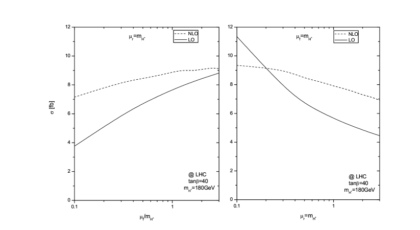
Figure 7: The dependence of the cross sections on factorization scale $\mu_{f}$ and renormalization scale $\mu_{r}$.

Fig.6 shows that our NLO QCD result does not depend on the arbitrary cutoffs $\delta_{s}$ and $\delta_{c}$ of the two cutoff phase space slicing method. The two-body($\sigma^{(2)}$) and three-body($\sigma^{(3)}$) contributions and the NLO cross section ($\sigma^{NLO}$) are shown as a function of the soft cutoff $\delta_{s}$ with the collinear cutoff $\delta_{c}=\delta_{s}/50$. $\tan\beta=40$, $m_{H^{\pm}}=180$ GeV and $\mu_{f}=\mu_{r}=m_{H^{\pm}}$. We can see the NLO cross section $\sigma^{NLO}$ is independent of the cutoffs. In the following numerical calculations, we take $\delta_{s}=10^{-4}$ and $\delta_{c}=\delta_{s}/50$.

In Fig.7, we show the dependence of the total cross section for $pp\to b\bar{b}\to H^{+}H^{-}+X$ on the renormalization scale and the factorization scale with $\tan\beta=40$, $m_{H^{\pm}}=180$ GeV. In the left plot of Fig.7, the renormalization scale is taken to be $\mu_{r}=m_{H^{\pm}}$ while the factorization scale varies in the region $0.1m_{H^{\pm}}\sim 3m_{H^{\pm}}$. In the right plot of Fig.7, we take $\mu_{f}=m_{H^{\pm}}$ and $0.1m_{H^{\pm}}<\mu_{r}<3m_{H^{\pm}}$. A significant reduction of the scale dependence for the NLO cross sections can be observed, thus the reliability of the NLO QCD predictions has been improved substantially.

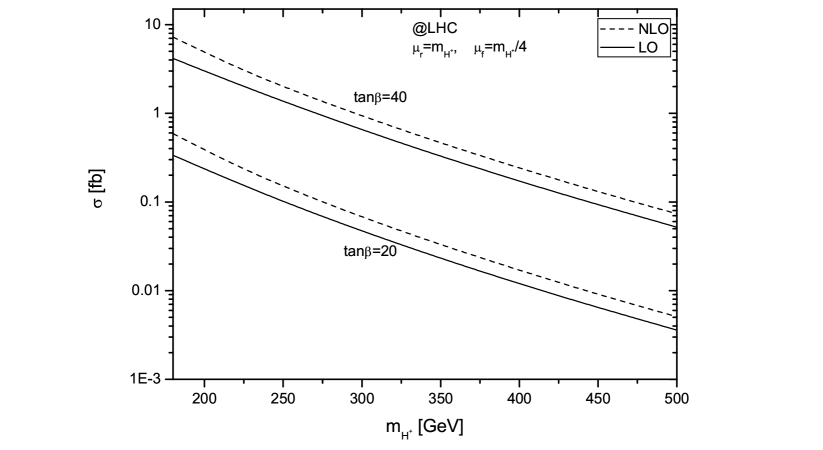
Figure 8: The dependence of the cross sections on $m_{H^{\pm}}$.

Figure 9: The dependence of the cross sections on $\tan\beta$.

Fig.8 shows the dependence of the LO and NLO cross sections for $pp\to b\bar{b}\to H^{+}H^{-}+X$ on the charged Higgs mass $m_{H^{\pm}}$. The values of $\tan\beta$ are taken to be 40 (upper lines) and 20 (lower lines). $m_{H^{\pm}}$ varies from 180 GeV to 500 GeV. The total cross section can reach 10 $fb$ for small values of $m_{H^{\pm}}$ with very large $\tan\beta$. In Fig.9, the dependence of the $pp\to b\bar{b}\to H^{+}H^{-}+X$ cross sections on $\tan\beta$ are studied for $m_{H^{\pm}}=180$ GeV and 400 GeV. The cross sections increase rapidly with the increment of $\tan\beta$ from 10 to 50.

IV..2 Results Including the Total SUSY QCD Corrections

In this subsection, we present the cross sections including all the NLO SUSY QCD corrections. The relevant SUSY parameters in our calculation are: the parameters $M_{\tilde{Q},\tilde{U},\tilde{D}}$ and $A_{t,b}$ in squark mass matrices, the higgsino mass parameter $\mu$ and the mass of the gluino $m_{\tilde{g}}$. The squark mass matrix is defined as

$${\cal M}_{\tilde{q}}^{2} = \left(\begin{array}[]{cc}m^{2}_{\tilde{q}_{L}}&a_{q}m_{q}\\ a_{q}m_{q}&m^{2}_{\tilde{q}_{R}}\end{array}\right)$$ (4.7)

with

$$m^{2}_{\tilde{q}_{L}} = M_{\tilde{Q}}^{2}+m_{q}^{2}+m_{Z}^{2}\cos 2\beta(I^{q}_{3}-e_{q}\sin^{2}\theta_{W}),$$

$$m^{2}_{\tilde{q}_{R}} = M_{\{\tilde{U},\tilde{D}\}}^{2}+m_{q}^{2}+m_{Z}^{2}\cos 2\beta e_{q}\sin^{2}\theta_{W}$$

$$a_{q} = A_{q}-\mu\{\cot\beta,\tan\beta\},$$ (4.8)

for {up, down} type squarks. $I_{3}^{q}$ and $e_{q}$ are the third component of the weak isospin and the electric charge of the quark $q$. The chiral states $\tilde{q}_{L}$ and $\tilde{q}_{R}$ are transformed into the mass eigenstates $\tilde{q}_{1}$ and $\tilde{q}_{2}$:

$$\left(\begin{array}[]{cc}\tilde{q}_{1}\\ \tilde{q}_{2}\end{array}\right)=R^{\tilde{q}}\left(\begin{array}[]{cc}\tilde{q}_{L}\\ \tilde{q}_{R}\end{array}\right),~{}~{}R^{\tilde{q}}=\left(\begin{array}[]{cc}\cos\theta_{\tilde{q}}&\sin\theta_{\tilde{q}}\\ -\sin\theta_{\tilde{q}}&\cos\theta_{\tilde{q}}\end{array}\right).$$ (4.9)

Then the mass eigenvalues $m_{\tilde{q}_{1}}$ and $m_{\tilde{q}_{2}}$ are given by

$$\left(\begin{array}[]{cc}m^{2}_{\tilde{q}_{1}}&0\\ 0&m^{2}_{\tilde{q}_{2}}\end{array}\right)=R^{\tilde{q}}{\cal M}_{\tilde{q}}^{2}(R^{\tilde{q}})^{\dagger}$$ (4.12)

For simplicity, we assume $M_{\tilde{Q}}=M_{\tilde{U}}=M_{\tilde{D}}=A_{t}=A_{b}=m_{\tilde{g}}\equiv M_{SUSY}=500$ GeV, $\mu=200$ GeV.

In the MSSM, the counter term of $m_{b}$ can be very large due to the ’pure’ SUSY QCD (gluino-mediated) diagram for large values of $\tan\beta$. The gluino-mediated contributions can be absorbed into the tree-level Yukawa couplings [21]. In such a way we obtain the $\overline{\rm MS}$ bottom quark mass $\overline{m}_{b}$ including the total SUSY QCD contributions,

$$(\overline{m}_{b}(\mu_{r}))^{SQCD}=(\overline{m}_{b}(\mu_{r}))^{QCD}-\frac{\alpha_{s}}{4\pi}C_{F}m_{b}\{\sum^{2}_{i=1}[B^{fin}_{1}-\frac{m_{\tilde{g}}}{m_{b}}\sin(2\theta_{\tilde{b}})(-1)^{i}B^{fin}_{0}](m^{2}_{b},m^{2}_{\tilde{g}},m^{2}_{\tilde{b}_{i}})\}$$

where the notations $B^{fin}_{1}$ and $B^{fin}_{0}$ denote the operations of taking the finite parts of the two-point integral functions. The $\mu_{r}$ dependence of $B$ functions cancels after summing over the sbottom index $i=1,2$. As shown in a series papers, the SUSY QCD contributions to the bottom quark running mass can be written as [22]

$$(\overline{m}_{b}(\mu_{r}))^{SQCD}\simeq\frac{(\overline{m}_{b}(\mu_{r}))^{QCD}}{1+\Delta m_{b}},$$ (4.14)

where

$$\Delta m_{b}=\frac{2\alpha_{s}}{3\pi}\mu m_{\tilde{g}}\tan\beta I(m_{\tilde{b}_{1}},m_{\tilde{b}_{2}},m_{\tilde{g}}),$$ (4.15)

with

$$I(a,b,c)=\frac{1}{(a^{2}-b^{2})(b^{2}-c^{2})(a^{2}-c^{2})}(a^{2}b^{2}\log\frac{a^{2}}{b^{2}}+b^{2}c^{2}\log\frac{b^{2}}{c^{2}}+c^{2}a^{2}\log\frac{c^{2}}{a^{2}}).$$ (4.16)

Indeed, if all supersymmetry breaking mass parameters and $\mu$ are of equal size, one get an interesting limit of Eq.(4.15)[23],

$$\Delta m_{b}=sign(\mu)\frac{\alpha_{s}(Q=M_{SUSY})}{3\pi}\tan\beta.$$ (4.17)

We can see $\Delta m_{b}$ does not decouple in the limit of large values of the supersymmetry breaking masses. The sign of $\mu$ is the decisive factor in determining whether the ’pure’ SUSY QCD corrections will enhance or suppress the cross section for the process of $pp\to b\bar{b}\to H^{+}H^{-}+X$.

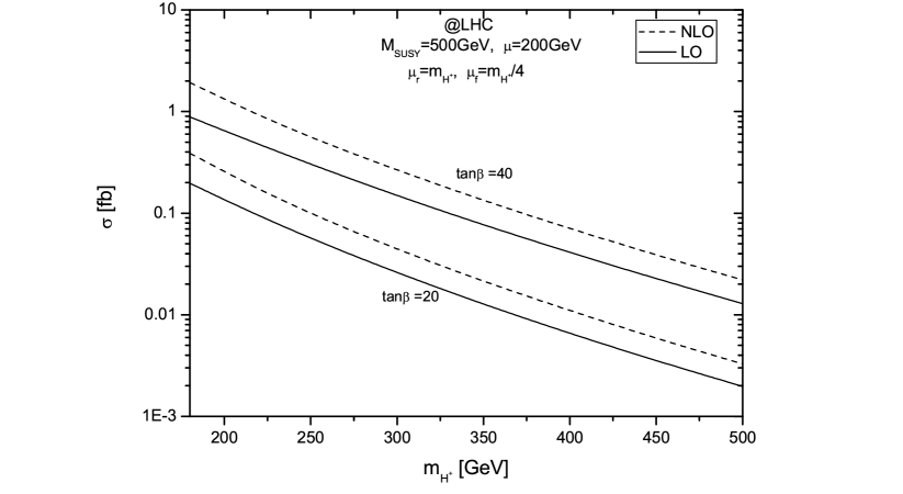
Figure 10: The dependence of the cross sections on $m_{H^{\pm}}$ including the total SUSY QCD corrections.

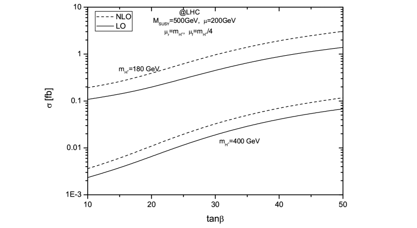
Figure 11: The dependence of the cross sections on $\tan\beta$ including the total SUSY QCD corrections.

In our calculations we use Eq.(IV..2) to calculate the $\overline{\rm MS}$ running bottom quark mass. The large SUSY QCD corrections are absorbed in the tree-level bottom Yukawa coupling, and we use the bottom quark mass counter term defined in Eq.(III..1) to avoid double counting. In Fig.10, we show the dependence of the LO and NLO cross sections on the charged Higgs mass $m_{H^{\pm}}$ which is same as Fig.8 but including the total SUSY QCD corrections. The curves in Fig.10 are much lower than those in Fig.8, because after including the ’pure’ SUSY QCD contributions $(\overline{m}_{b}(\mu_{r}))^{SQCD}$ is much smaller than $(\overline{m}_{b}(\mu_{r}))^{QCD}$, assuming the sign of $\mu$ is positive and $\tan\beta$ is large (see Eq.(4.17)). In Fig.11, we plot the $\tan\beta$ dependence of the cross section including the total SUSY QCD contributions.

In summary, we have studied the production of the charged Higgs boson pair via the bottom quark fusion in the MSSM including the NLO QCD contributions at the LHC. With very large values of $\tan\beta$, $b\bar{b}\to H^{+}H^{-}$ subprocess can become the dominant mechanism in the charged Higgs boson pair production at the LHC. The numerical results of the cross sections show that the NLO SUSY QCD corrections are generally significant. We find also that the $\overline{\rm MS}$ bottom quark mass $\overline{m}_{b}$ will receive large corrections from the ’pure’ SUSY QCD contributions which will significantly suppress or enhance the cross section depending on the sign of the higgsino mass parameter $\mu$. The NLO QCD corrections can significantly reduce the dependence of the cross sections on the renormalization and factorization scales.

Acknowledgments: This work was supported in part by the National Natural Science Foundation of China and special fund sponsored by China Academy of Science.

References

• [1] S. Weinberg, Phys. Rev. Lett. 19, 1264 (1967); S. Glashow, Nucl. Phys. B 22, 579 (1961); A. Salam, in $Elementary$ $Particle$ $Theory$, edited by N. Svartholm, p367 (1968).
• [2] H. P. Nilles Phys. Rep. 110, 1 (1984); H. E. Haber and G. L. Kane, Phys. Rep. 117, 75 (1985); J. F. Gunion, H. E. Haber, Nucl. Phys. B 272, 1 (1986).
• [3] Z. Kunszt and F. Zwirner, Nucl.Phys. B 385, 3 (1992).
• [4] J. F. Gunion, H. E. Haber, F. E. Paige, W.-K. Tung and S. S. D. Willenbrock, Nucl. Phys. B 294, 621 (1987); R. M . Barnett, H. E. Haber and D. E. Soper Nucl. Phys. B 306, 697 (1988); F. I. Olness and W.-K. Tung, Nucl. Phys. B 308, 813 (1988); V. Barger, R. J. N. Philips and D. P. Roy, Phys. Lett. B 324, 236 (1994).
• [5] J. L. Diaz-Cruz and O. A. Sampayo, Phys. Rev. D 50, 6820 (1994).
• [6] S. Moretti and K. Odagiri, Phys. Rev. D 55, 5627 (1997).
• [7] D. A. Dicus, J. L. Hewett, C. Kao and T. G. Rizzo, Phys. Rev. D 40, 787 (1989); S. Moretti and K. Odagiri, Phys. Rev. D 59, 055008 (1999); A.A.Barrientos Bendezu and B. A. Kniehl, Phys. Rev. D 59, 015009 (1998); A.A.Barrientos Bendezu and B. A. Kniehl, Phys. Rev. D 61, 097701 (2000); A.A.Barrientos Bendezu and B. A. Kniehl, Phys. Rev. D 63, 015009 (2000); O. Brein, W. Hollik, and S. Kanemura, Phys. Rev. D 63, 095001 (2001).
• [8] E. Eichten, I. Hinchliffe, K. Lane and C. Quigg, Rev. Mod. Phys. 56, 579 (1984).
• [9] A.A. Barrientos Bendezú and B.A. Kniehl, Nucl. Phys. B 568, 305 (2000);
• [10] S.S.D. Willenbrock, Phys. Rev. D 35, 173 (1987); Y. Jiang, W.-G. Ma, L. Han, M. Han and Z.-H. Yu, J. Phys. G 23, 385 (1997), Erratum, ibidem G 23, 1151 (1997); A. Krause, T. Plehn, M. Spira and P.M. Zerwas, Nucl. Phys. B 519, 85 (1998); A. Belyaev, M. Drees, O.J.P. Eboli, J.K. Mizukoshi and S.F. Novaes, Phys. Rev. D 60, 075008 (1999); A. Belyaev, M. Drees and J.K. Mizukoshi, Eur. Phys. J. C 17, 337 (2000); O. Brein and W. Hollik, Eur. Phys. J. C 13, 175 (2000).
• [11] S. Moretti, J. Phys. G 28, 2567 (2002).
• [12] S. Moretti and J. Rathsman, Eur. Phys. J. C 33, 41 (2004).
• [13] D. Rainwater, M. Spira and D. Zeppenfeld, MAD-PH-02-1260, hep-ph/0203187; M. Spira, PSI-PR-02-19, hep-ph/0211145.
• [14] T. Plehn, Phys. Rev. D 67, 014018 (2003); F. Maltoni, Z. Sullivan and S. Willenbrock, Phys. Rev. D 67, 093005 (2003); E. Boos and T. Plehn, Phys.Rev. D 69, 094005 (2004); R. V. Harlander and W. B. Kilgore, Phys.Rev. D 68, 013001 (2003).
• [15] K. Fabricius, I. Schmitt, G. Kramer and G. Schierholz, Z. Phys. C 11, 315(1981); G. Kramer and B. Lampe, Fortschr. Phys. 37, 161(1989); W. T. Giele and E.W.N. Glover, Phys. Rev. D 46, 1980(1992); W. T. Giele, E.W.N. Glover and D.A. Kosower, Nucl. Phys. B 403, 633 (1993).
• [16] B.W. Harris and J.F. Owens, Phys. Rev. D 65 094032(2002)
• [17] G.P. Lepage, J. Comput. Phys. 27,192(1978)
• [18] G. Altarelli and G. Parisi, Nucl. Phys. B126 298 (1977).
• [19] S. Eidelman, et al., Phys. Lett. B529, (2004)1.
• [20] J. Pumplin et al., JHEP 0207, 012 (2002); D. Stump et al., JHEP 0310, 046 (2003).
• [21] C. Weber, H. Eberl, W. Majerotto, Phys.Rev. D 68, 093011(2003).
• [22] L.J. Hall, R. Rattazzi and U. Sarid, Phys. Rev. D50, 7048 (1994); M. Carena, M. Olechowski, S. Pokorski and C. E. Wagner, Nucl. Phys. B 426, 269 (1994); D. Pierce, J. Bagger, K. Matchev and R. Zhang, Nucl. Phys. B 491, 3(1997).
• [23] M. Carena, D. Garcia, U. Nierste and C.E. Wagner, Nucl. Phys. B 577, 88 (2000).