Upper Bounds on Lepton-number Violating Processes

Abstract

We consider four lepton-number violating ($\not{\hbox{\kern-4.0pt$L$}}$) processes: (a) neutrinoless double-beta decay $(0\nu\beta\beta)$, (b) $\Delta L=2$ tau decays, (c) $\Delta L=2$ rare meson decays and (d) nuclear muon-positron conversion. In the absence of exotic $\not{\hbox{\kern-4.0pt$L$}}$ interactions, the rates for these processes are determined by effective neutrino masses $\left<m\right>_{\ell_{1}\ell_{2}}$, which can be related to the sum of light neutrino masses, the neutrino mass-squared differences, the neutrino mixing angles, a Dirac phase and two Majorana phases. We sample the experimentally allowed ranges of $\left<m\right>_{\ell_{1}\ell_{2}}$ based on neutrino oscillation experiments as well as cosmological observations, and obtain a stringent upper bound $\left<m\right>_{\ell_{1}\ell_{2}}\mathrel{\raise 1.29167pt\hbox{$<$\kern-7.5pt\lower 4.30554pt\hbox{$\sim$}}}0.14$ eV. We then calculate the allowed ranges for $\left<m\right>_{\ell_{1}\ell_{2}}$ from the experimental rates of direct searches for the above $\Delta L=2$ processes. Comparing our calculated rates with the currently or soon available data, we find that only the $0\nu\beta\beta$ experiment may be able to probe $\left<m\right>_{ee}$ with a sensitivity comparable to the current bound. Muon-positron conversion is next in sensitivity, while the limits of direct searches for the other $\Delta L=2$ processes are several orders of magnitude weaker than the current bounds on $\left<m\right>_{\ell_{1}\ell_{2}}$. Any positive signal in those direct searches would indicate new contributions to the $\not{\hbox{\kern-4.0pt$L$}}$ interactions beyond those from three light Majorana neutrinos.

I Introduction

Fermion masses and flavor mixing are among the most mysterious problems of contemporary particle physics and they have posed major challenges to particle theory and experiment for decades. Further understanding of these issues should eventually shed light on fundamental phenomena like CP violation, flavor-changing neutral currents, baryon-number ($B$) and lepton-number ($L$) asymmetry in the Universe and will hopefully lead to a more satisfactory unified theory of flavor physics [1].

In the Standard Model (SM) of strong and electroweak interactions, neutrinos are strictly massless due to the absence of the right-handed chiral states ($\nu_{R}$) and the requirement of $SU(2)_{L}$ gauge invariance and renormalizability. Recent neutrino oscillation experiments have conclusively shown that neutrinos are massive [2]. This discovery presents a pressing need to consider physics beyond the Standard Model. It is straightforward to introduce a Dirac mass term $m_{D}(\overline{\nu_{L}}\nu_{R}+$h.c.) for a neutrino by including the right-handed state, just like the treatment for all other fermions via the Yukawa couplings to the Higgs doublet in the SM. However, a profound question arises: Since $\nu_{R}$ is a SM gauge singlet, why should not there exist a gauge-invariant Majorana mass term ${1\over 2}M\nu_{R}\nu_{R}$ in the theory? In fact, there is a strong theoretical motivation for the Majorana mass term to exist since it could naturally explain the smallness of the observed neutrino masses via the so-called “see-saw” mechanism $m_{\nu}\approx m^{2}_{D}/M$ [3]. From a model-building point of view, there are many scenarios that could incorporate the Majorana mass. Examples include R-parity violating interactions ($\Delta L=1$) in Supersymmetry (SUSY) [4], Left-Right symmetric gauge theories [5], grand unified theories [6], models with exotic Higgs representations [7, 8] and theories with extra dimensions [9]. One may also consider constructing generic neutrino mass operators to parameterize the fundamental physics effects in a model-independent manner [10].

Besides the phenomena of neutrino flavor oscillations and possible new CP-violating phases, the Majorana mass term violates lepton number by two units ($\Delta L=2$), which may result in important consequences in particle physics and cosmology. Although the prevailing theoretical prejudice prefers Majorana neutrinos, experimentally testing the nature of the neutrinos, and lepton-number violation ($\not{\hbox{\kern-4.0pt$L$}}$) in general, is of fundamental importance. The basic process with $\Delta L=2$ is mediated by

$$W^{-}W^{-}\rightarrow\ell^{-}_{1}\ell^{-}_{2},$$

where the $W^{-}$ are virtual SM weak bosons and $\ell_{1,2}=e,\ \mu,\ \tau$. By coupling fermion currents to the $W$ bosons as depicted in Fig. 1, and arranging the initial and final states properly, one finds various physical processes that can be experimentally searched for. The best known example is the neutrinoless double-beta decay ($0\nu\beta\beta$) [11, 12, 13], which proceeds via the parton-level subprocess $dd\to uu\ W^{-*}W^{-*}\to uu\ e^{-}e^{-}$. Other interesting classes of $\not{\hbox{\kern-4.0pt$L$}}$ processes involve tau decays such as $\tau^{-}\to e^{+}(\mu^{+})\pi^{-}\pi^{-}$ etc. [14] and hyperon decays such as $\Sigma^{-}\to\Sigma^{+}e^{-}e^{-}$, $\Xi^{-}\to p\mu^{-}\mu^{-}$ etc. [15]. One could also explore additional processes like $e^{-}\to\mu^{+}$ conversion [16] . One may also consider searching for signals at accelerator and collider experiments via $e^{-}e^{-}\to W^{-}W^{-}$ [17], $e^{\pm}p\to\nu_{e}(\bar{\nu}_{e})\ell_{1}^{\pm}\ell_{2}^{\pm}X$ [18], $\nu_{\ell}(\bar{\nu}_{\ell})N\to\ell^{\mp}\ell_{1}^{\pm}\ell_{2}^{\pm}X$ [19] and $pp\to\ell^{+}_{1}\ell^{+}_{2}X$ [20].

Figure 1: A generic diagram for $\Delta L=2$ processes via Majorana neutrino exchange.

Assuming no additional contributions from other exotic particles that have $\not{\hbox{\kern-4.0pt$L$}}$ interactions, the matrix element for $\not{\hbox{\kern-4.0pt$L$}}$ processes is proportional to the product of two flavor mixing matrix elements and a $\not{\hbox{\kern-4.0pt$L$}}$ mass insertion from a light Majorana neutrino

$$\left<m\right>_{\ell_{1}\ell_{2}}=|\sum_{i}V_{\ell_{1}i}V_{\ell_{2}i}m_{i}|.$$

The $\left<m\right>_{\ell_{1}\ell_{2}}$ are called “effective neutrino masses”. Experimental searches for $\not{\hbox{\kern-4.0pt$L$}}$ processes will directly measure the effective neutrino masses squared, and thus probe the fundamental parameters of neutrino mixing angles and phases and their masses.

In this paper we study $\Delta L=2$ processes related to $W^{-}W^{-}\rightarrow\ell_{1}^{-}\ell_{2}^{-}$. We establish our conventions and lay out the general expressions for the effective neutrino masses in Sec. II. We then calculate those quantities, based on the current knowledge from atmospheric, solar and reactor neutrino oscillation experiments. We include the constraints on neutrino masses from a joint analysis of Wilkinson Microwave Anisotropy Probe (WMAP), Cosmic Microwave Background (CMB) data, the Sloan Digital Sky Survey (SDSS) large scale galaxy survey and bias, the SDSS Ly$\alpha$ forest power spectrum and the latest supernovae SNIa sample. We thereby limit the allowed ranges of the $\left<m\right>_{\ell_{1}\ell_{2}}$. In Sections III, IV, V, and VI we study the four $\Delta L=2$ processes,

• neutrinoless double-beta decay ($0\nu\beta\beta$),

• $\not{\hbox{\kern-4.0pt$L$}}$ tau decays $\tau^{-}\rightarrow\ell^{+}M_{1}^{-}M_{2}^{-}$,

• $\not{\hbox{\kern-4.0pt$L$}}$ meson decays $M_{1}^{+}\rightarrow M_{2}^{-}\ell_{1}^{+}\ell_{2}^{+}$,

• nuclear muon-positron ($\mu^{-}-e^{+}$) conversion.

We calculate the transition rates and determine the allowed ranges of $\left<m\right>_{\ell_{1}\ell_{2}}$ from the bounds set by direct experimental searches for the above $\Delta L=2$ processes, and then compare the results with the bounds obtained based on the neutrino mixing inputs in Sec. II. We find that the upper bound from $0\nu\beta\beta$ is most sensitive to the model-parameters and is at the same level as the constraint from Sec. II. The bounds from the other three classes of measurements are significantly weaker although they probe different combinations of the parameters. In the future should we observe a $\not{\hbox{\kern-4.0pt$L$}}$ signal in one of those channels, it would indicate non-standard physics beyond the contributions of light Majorana neutrinos. We draw our conclusions in Sec. VII. Some technical details in calculating the transition rates for the above processes are presented in the Appendices.

II Effective Neutrino Masses

In terms of neutrino mass eigenstates $\nu_{i}$ the charged current interaction Lagrangian is written as

$${\cal L}_{cc}=-\frac{g}{\sqrt{2}}\sum_{\ell=e,\mu,\tau}{\sum_{i=1,2,3}}V_{\ell i}{\bar{\ell}}\gamma^{\mu}P_{L}\nu_{i}W_{\mu}+{\rm h.c.}$$ (1)

where $P_{L}$ is the left-handed projection operator $(1-\gamma_{5})/2$, $V_{\ell i}$ is the Maki-Nakamura-Sakata-Pontecorvo (MNSP) mixing matrix element [21] between the lepton mass eigenstate $\ell=e,\mu,\tau$ and the $i^{th}$ neutrino mass eigenstate. It is conveniently parameterized by [2]

$$V=\left(\matrix{c_{s}c_{x}&s_{s}c_{x}e^{i\frac{\phi_{2}}{2}}&s_{x}e^{i\frac{\phi_{3}}{2}}\cr-s_{s}c_{a}-s_{a}s_{x}c_{s}e^{i\delta}&c_{a}c_{s}e^{i\frac{\phi_{2}}{2}}-s_{a}s_{s}s_{x}e^{i\frac{\phi_{2}}{2}}e^{i\delta}&s_{a}c_{x}e^{i\frac{\phi_{3}}{2}}e^{i\delta}\cr s_{a}s_{s}-s_{x}c_{a}c_{s}e^{i\delta}&-s_{a}c_{s}e^{i\frac{\phi_{2}}{2}}-s_{s}s_{x}c_{a}e^{i\frac{\phi_{2}}{2}}e^{i\delta}&c_{a}c_{x}e^{i\frac{\phi_{3}}{2}}e^{i\delta}\cr}\right)$$ (2)

in the notation $c_{i}$ = cos$\theta_{i}$ and $s_{i}$ = sin$\theta_{i}$. The mixing angles $\theta_{a}$ and $\theta_{s}$ are relevant to atmospheric and solar oscillations, respectively, and the angle $\theta_{x}$ is presently unknown, except that it is bounded by the CHOOZ reactor data. The phase $\delta$ is a Dirac phase and $\phi_{2}$, $\phi_{3}$ are Majorana phases.

The general subprocess of $\not{\hbox{\kern-4.0pt$L$}}$ is neutrinoless dilepton production from two virtual $W$ bosons as depicted in Fig. 1

$$W^{-}W^{-}\rightarrow\ell^{-}_{1}\ell^{-}_{2},$$ (3)

which can occur only if neutrinos are Majorana particles. This subprocess changes the lepton number from $L=0$ to $L=2$ and the observation of $\not{\hbox{\kern-4.0pt$L$}}$ would establish that neutrino is a Majorana particle. The leptonic subprocess of Eq. (3) occurs via Majorana neutrino exchange and is given by the product of two charged currents

$${{\cal M}_{lep}^{\mu\nu}}\propto{\sum_{i}}V_{\ell_{1}i}V_{\ell_{2}i}({\bar{\ell}_{1}}\gamma^{\mu}P_{L}\nu_{i})({\bar{\ell}_{2}}\gamma^{\nu}P_{L}\nu_{i}).$$ (4)

As presented in Appendix A, the transition rates for light neutrino exchange are proportional to the squares of effective neutrino masses $\left<m\right>_{\ell_{1}\ell_{2}}$ defined as

$$\left<m\right>_{\ell_{1}\ell_{2}}={\mid}\sum_{i}V_{\ell_{1}i}V_{\ell_{2}i}m_{i}\mid,$$ (5)

where $\ell_{1},\ell_{2}=e,\mu,\tau,\ i=1,2,3$. Since the mixing factor is symmetric $V_{\ell_{1}i}V_{\ell_{2}i}=V_{\ell_{2}i}V_{\ell_{1}i}$, there are six different $\left<m\right>_{\ell_{1}\ell_{2}}$. The explicit expressions for $\left<m\right>_{\ell_{1}\ell_{2}}$ are given [22] by

$$\left<m\right>_{ee} = |m_{1}c_{s}^{2}c_{x}^{2}+m_{2}s_{s}^{2}c_{x}^{2}e^{i\phi_{2}}+m_{3}s_{x}^{2}e^{i\phi_{3}}|,$$

$$\left<m\right>_{e\mu} = |m_{1}c_{s}c_{x}(-s_{s}c_{a}-s_{a}s_{x}c_{s}e^{i\delta})+m_{2}s_{s}c_{x}(c_{a}c_{s}e^{i\phi_{2}}-s_{a}s_{s}s_{x}e^{i(\phi_{2}+\delta)})+m_{3}s_{a}s_{x}c_{x}e^{i(\phi_{3}+\delta)}|,$$

$$\left<m\right>_{e\tau} = |m_{1}c_{s}c_{x}(s_{a}s_{s}-s_{x}c_{a}c_{s}e^{i\delta})+m_{2}s_{s}c_{x}(-s_{a}c_{s}e^{i\phi_{2}}-s_{s}s_{x}c_{a}e^{i(\phi_{2}+\delta)})+m_{3}s_{x}c_{a}c_{x}e^{i(\phi_{3}+\delta)}|,$$

$$\left<m\right>_{\mu\mu} = |m_{1}(s_{s}c_{a}+s_{a}s_{x}c_{s}e^{i\delta})^{2}+m_{2}(c_{a}c_{s}e^{i\frac{\phi_{2}}{2}}-s_{a}s_{s}s_{x}e^{i(\frac{\phi_{2}}{2}+\delta)})^{2}+m_{3}s_{a}^{2}c_{x}^{2}e^{i(\phi_{3}+2\delta)}|,$$

$$\left<m\right>_{\mu\tau} = |m_{1}(s_{s}c_{a}+s_{a}s_{x}c_{s}e^{i\delta})(s_{x}c_{a}c_{s}e^{i\delta}-s_{a}s_{s})+m_{3}s_{a}c_{a}c_{x}^{2}e^{i(\phi_{3}+2\delta)}$$

$$+ m_{2}(s_{a}s_{s}s_{x}e^{i(\phi_{2}+\delta)}-c_{a}c_{s}e^{i\phi_{2}})(s_{a}c_{s}+s_{s}s_{x}c_{a}e^{i\delta})|,$$

$$\left<m\right>_{\tau\tau} = |m_{1}(s_{a}s_{s}-s_{x}c_{a}c_{s}e^{i\delta})^{2}+m_{2}(-s_{a}c_{s}e^{i\frac{\phi_{2}}{2}}-s_{s}s_{x}c_{a}e^{i(\frac{\phi_{2}}{2}+\delta)})^{2}+m_{3}c_{a}^{2}c_{x}^{2}e^{i(\phi_{3}+2\delta)}|.$$ (6)

We can see that the $\left<m\right>_{\ell_{1}\ell_{2}}$ are functions of the oscillation angles ($\theta_{a},\theta_{s}\mbox{ and }\theta_{x}$) and the neutrino masses $m_{i}$. The three neutrino masses can be expressed in terms of other three measured quantities: the sum of neutrino masses and the two mass-squared differences,

$$\Sigma=m_{1}+m_{2}+m_{3}=m_{1}+\sqrt{m_{1}^{2}+\delta m^{2}_{s}}+\sqrt{m_{1}^{2}+\delta m^{2}_{a}}.$$ (7)

The atmospheric ($a$) and solar ($s$) mass-squared differences are defined as

$$\delta m^{2}_{a} = m^{2}_{3}-m^{2}_{1},$$

$$\delta m^{2}_{s} = m^{2}_{2}-m^{2}_{1},$$ (8)

where $\delta m^{2}_{a}>0$ for the normal hierarchy (NH) and $\delta m^{2}_{a}<0$ for the inverted hierarchy (IH).

The above expressions provide a convenient formalism to study the range of values of $\left<m\right>_{\ell_{1}\ell_{2}}$ as functions of the angles and the phases (both Dirac and Majorana). In particular, we study $\Sigma$ versus $\left<m\right>_{\ell_{1}\ell_{2}}$ for both the normal and inverted hierarchies. To do this in a comprehensive manner, we carry out a Monte Carlo sampling of the oscillation parameters and phases. The Dirac phase ($\delta$) and the two Majorana phases ($\phi_{2}$ and $\phi_{3}$) are allowed to range between $0$ and 2$\pi$. The atmospheric oscillation data gives bounds on [23]

$$1.9\times 10^{-3}\mbox{ eV}^{2}<|\delta m^{2}_{a}|<3.0\times 10^{-3}\mbox{ eV}^{2},\ \sin^{2}2\theta_{a}>0.9\ {\rm at}\ 90\%\ {\rm CL}.$$

In fact, the bounds on $\theta_{a}$ vary with $\delta m^{2}_{a}$ and in our computation these bounds are obtained from the 90$\%$ CL $\delta m^{2}_{a}$ versus sin${}^{2}2\theta_{a}$ plot of Ref. [24], which was obtained in an $L/E$ analysis of only selected high resolution FC (fully contained) and PC (partially contained) events. The analysis of the full data set from the same running period [25] gives slightly different constraints; the constraints on sin${}^{2}2\theta_{a}$ are slightly better from the full data set but the $L/E$ analysis better constrains $\delta m^{2}_{a}$. Similarly, for the above range of $\delta m^{2}_{a}$, reactor data places bounds on

$$\sin^{2}\theta_{x}<0.06,$$

which also vary with $\delta m^{2}_{a}$. We use the limits obtained from the CHOOZ 90$\%$ CL exclusion plot of Ref. [26]. Finally a joint analysis of the solar and reactor oscillation data limits the parameter ranges to

$$7.6\times 10^{-5}\ \mbox{eV}^{2}<\delta m^{2}_{s}<9.1\times 10^{-5}\ \mbox{eV}^{2},\ {\rm and}\ 0.31<\tan^{2}\theta_{s}<0.52\ {\rm at}\ 90\%\ {\rm CL.}$$

The bounds on $\theta_{s}$ vary with $\delta m^{2}_{s}$ and these are obtained from the 90$\%$ CL $\delta m^{2}_{s}$ versus tan${}^{2}\theta_{s}$ plot of Ref. [27]. All the inputs to the Monte Carlo sampling are summarized in Table I. We can further constrain the range of $\left<m\right>_{\ell_{1}\ell_{2}}$ by imposing limits on $\Sigma$ obtained from cosmology. The current best limit

$$\Sigma\leq\mbox{0.42 eV at }95\%\mbox{ CL}$$ (9)

was obtained from an analysis of WMAP, the SDSS galaxy spectrum and its bias, the SDSS Ly$\alpha$ forest power spectrum and the latest supernovae SNIa sample, assuming a spatially flat universe and adiabatic initial conditions [28]. Throughout this paper, we will adopt the cosmological bound of Eq. (9). We would like to point out that more conservative analyses without including the Ly$\alpha$ forest power spectrum exist. These lead to larger values of $\Sigma$, such as $\Sigma\leq\mbox{0.75 eV}$ [29] and $\Sigma\leq\mbox{0.54 eV}$ [30] at the 2$\sigma$ level.

Table 1: Inputs to Monte Carlo sampling for calculating effective neutrino masses

Parameter	Input
$|\delta m_{a}^{2}|$	$1.9\times 10^{-3}\mbox{ eV}^{2}-3.0\times 10^{-3}\mbox{ eV}^{2}$ [23]
$\delta m_{s}^{2}$	90$\%$ CL $\delta m^{2}_{s}$ versus tan${}^{2}\theta_{s}$ plot [27]
$\theta_{a}$	90$\%$ CL $\delta m^{2}_{a}$ versus sin${}^{2}2\theta_{a}$ plot [24]
$\theta_{s}$	90$\%$ CL $\delta m^{2}_{s}$ versus tan${}^{2}\theta_{s}$ plot [27]
$\theta_{x}$	CHOOZ 90$\%$ CL exclusion plot [26]
$\delta$	0 to 2$\pi$
$\phi_{2}$	0 to 2$\pi$
$\phi_{3}$	0 to 2$\pi$

The results of the Monte Carlo sampling along with constraints from cosmology are shown in Fig. 2 for both normal and inverted hierachies by solid and dashed curves respectively. We first point out the following general features:

• For large values of the minimum neutrino mass, typically $m_{min}>0.1$ eV, the mass differences are unimportant and thus $m_{1}\approx m_{2}\approx m_{3}$ or $\Sigma\mathrel{\raise 1.29167pt\hbox{$>$\kern-7.5pt\lower 4.30554pt\hbox{$\sim$}}}3m_{min}$. Due to unitarity of the mixing matrix, we can see that the maximum values of effective masses obey $\left<m\right>_{\ell_{1}\ell_{2}}\approx m_{min}\mathrel{\raise 1.29167pt\hbox{$<$\kern-7.5pt\lower 4.30554pt\hbox{$\sim$}}}\Sigma/3.$ On the other hand, for smaller values of $m_{min}$, $\Sigma$ is governed by the larger mass difference, namely $\Sigma\mathrel{\raise 1.29167pt\hbox{$>$\kern-7.5pt\lower 4.30554pt\hbox{$\sim$}}}\sqrt{\delta m^{2}_{a}}\approx m_{3}\approx 5\times 10^{-2}$ eV for the NH scenario, and $\Sigma\mathrel{\raise 1.29167pt\hbox{$>$\kern-7.5pt\lower 4.30554pt\hbox{$\sim$}}}2\sqrt{\delta m^{2}_{a}}\approx 2m_{1}\approx 9\times 10^{-2}$ eV for the IH scenario.

• The cosmological observations of $\Sigma\leq$ 0.42 eV put an upper limit on $\left<m\right>_{\ell_{1}\ell_{2}}$ at about 0.14 eV.

• The normal and inverted hierarchies are indistinguishable at the current level of sensitivity. When $\Sigma$ is smaller than the present cosmology limit, the difference (in upper limits) between normal and inverted hierarchies may become significant as is apparent from all the plots. We are just above the region where the NH and IH results begin to separate. An improvement in the accuracy of either of the two observables by a factor of two or better would begin to provide a sensitive probe to distinguish the NH and IH scenarios.

We note the qualitative difference between Fig. 2(a) and the other panels in Fig. 2. The allowed region for ${\left<m\right>_{ee}}$ is between the curves for both normal hierarchy (solid lines) and inverted hierarchy (dashed curves). It is more stringent than the other ${\left<m\right>_{\ell_{1}\ell_{2}}}$ because ${\left<m\right>_{ee}}$ depends on two fewer parameters ($\theta_{a},\ \delta$) than the others. Also the specific combination of oscillation parameters for ${\left<m\right>_{ee}}$ does not lead to complete cancellations or vanishingly small contributions (unless for a small range of $\Sigma$ in the NH scenario) unlike others. Our results for the range of values of ${\left<m\right>_{ee}}$ are similar to the analyses previously done in Refs. [31, 32] and an updated version presented in Ref. [33]. Similar analyses for the other $\left<m\right>_{\ell_{1}\ell_{2}}$ for specific scenarios were considered in Ref. [34]. We will not show the results for $\left<m\right>_{e\mu}$ and $\left<m\right>_{\tau\tau}$ since they are qualitatively very similar to $\left<m\right>_{e\tau}$ and $\left<m\right>_{\mu\mu}$, respectively.

By setting limits on the $\not{\hbox{\kern-4.0pt$L$}}$ process decay rates and cross sections, direct experimental upper bounds on effective neutrino masses can be obtained as to be discussed in the next sections. We then compare them with the results from this section.

III Neutrinoless double-beta decay $(0\nu\beta\beta)$

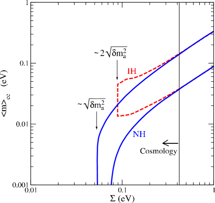
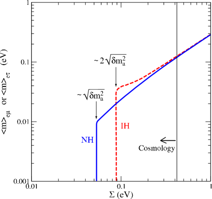
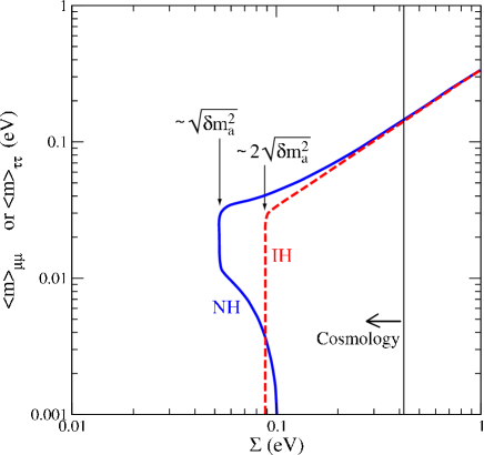
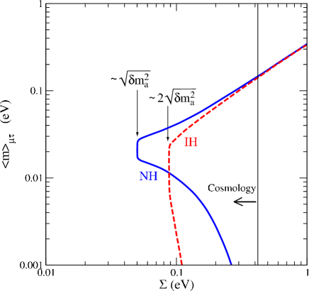
Figure 2: (a) Upper left: allowed regions between the curves for $\left<m\right>_{ee}$ versus $\Sigma$; (b) upper right: allowed regions to the right of the curves for $\left<m\right>_{e\mu}$ or $\left<m\right>_{e\tau}$; (c) lower left: same as (b) but for $\left<m\right>_{\mu\mu}$ or $\left<m\right>_{\tau\tau}$; (d) lower right: same as (b) but for $\left<m\right>_{\mu\tau}$. The bound for $\Sigma$ at 95$\%$ CL from cosmology is shown in all figures by the vertical line.

The decay rate for neutrinoless double-beta decay $(0\nu\beta\beta)$ is proportional to ${\left<m\right>^{2}_{ee}}$; ${\left<m\right>_{ee}}$ is plotted in Fig. 2(a). The theoretical formalism for calculating the decay rate is given in Appendix B. Ref. [12] summarized the latest experimental limits of $0\nu\beta\beta$ for various isotopes; the results are reproduced in Table 2. The experimental bound on $\left<m\right>_{ee}$ has improved from 5 eV in 1992 to about 1 eV in the most recent experiments. The best limits come from the two ⁷⁶Ge experiments which are Heidelberg-Moscow and IGEX respectively. Although $0\nu\beta\beta$ is a vital experiment to determine the Majorana nature of neutrinos, we note that the uncertainty in nuclear matrix elements would result in an uncertainty as large as a factor of three in the inferred value of $\left<m\right>_{ee}$ from an observation of the decay process [12].

We list our result in the last row of Table 2 based on Fig. 2(a) which is largely determined by the cosmological bound. We see that our result is slightly stronger than the current experimental bounds. The bounds we obtain for $\left<m\right>_{ee}$ are based on the Monte Carlo scan over the fundamental parameters in the neutrino sector as given in Table 1 and thus are independent of the nuclear matrix elements. The large uncertainty comes in when we predict the decay rates for the nuclear isotopes.

Table 2: Experimental bounds on half-life time of $0\nu\beta\beta$ for various isotopes from Ref. [12] and the implied upper bounds on $\left<m\right>_{ee}$. The last row lists the cosmological bound as obtained in the previous section.

Isotope	Half-life (years)	$\left<m\right>_{ee}$ (eV)	Year of published paper
48Ca	$>1.4\times 10^{22}$	$<7.2-44.7$	2004
76Ge	$>1.9\times 10^{25}$	$<0.35$	2001
76Ge	$>1.6\times 10^{25}$	$<0.33-1.35$	2002
76Ge	$=1.2\times 10^{25}$	$=0.44$	2004
82Se	$>2.7\times 10^{22}$	$<5$	1992
100Mo	$>5.5\times 10^{22}$	$<2.1$	2001
116Cd	$>1.7\times 10^{23}$	$<1.7$	2003
128Te	$>7.7\times 10^{24}$	$<1.1-1.5$	1993
130Te	$>5.5\times 10^{23}$	$<0.37-1.9$	2004
136Xe	$>4.4\times 10^{23}$	$<1.8-5.2$	1998
150Nd	$>1.2\times 10^{21}$	$<3$	1997
Cosmology	none	$\leq 0.14$	this paper

A recent publication claims evidence for $0\nu\beta\beta$ at the $4.2\sigma$ level [35], but the result is controversial. In Ref. [35], $\left<m\right>_{ee}$ was determined to be in a range between 0.2 to 0.6 eV at 99.73$\%$ CL for a particular choice of the nuclear matrix element, and becomes 0.1 to 0.9 eV if allowing a $\pm 50\%$ uncertainty of the nuclear matrix element. With the bound on $\Sigma$ at 95$\%$ CL, the first range is disfavored by the limits we obtained and the second range allowing a larger uncertainty leaves a very narrow range for ${\left<m\right>_{ee}}$.

Tritium $\beta$ decay experiments also probe the absolute scale of the neutrino mass. The current limits from cosmology are better by an order of magnitude compared to the tritium $\beta$ decay limits [33]. Future limits from the KATRIN tritium $\beta$-decay experiment are expected to be 0.30 eV (0.35 eV) at the 3$\sigma$ (5$\sigma$) level. The present limit on $\left<m\right>_{ee}$ from cosmology is still stronger than this expected improvement from KATRIN, but the KATRIN experiment will provide an important direct confirmation.

IV Lepton-number violating tau decay

In this section we examine tau decays into an anti-lepton and two mesons

$$\tau^{-}\rightarrow\ell^{+}M_{1}^{-}M_{2}^{-},$$ (10)

which is a process with $\Delta L=-2$. The relevant effective masses are $\left<m\right>_{e\tau}$ and $\left<m\right>_{\mu\tau}$ as shown in Fig. 2(b) and Fig. 2(d) respectively, from the current parameters from neutrino oscillation experiments. The constraint from cosmology of Eq. (9) gives an upper limit of 0.14 eV for $\left<m\right>_{e\tau}$ and $\left<m\right>_{\mu\tau}$. In Appendix C, we give the calculations for the decay branching fraction of the process (10) in terms of $\left<m\right>^{2}_{\ell\tau}$. We express the branching fraction in an intuitive form as

$$BR\approx 10^{-33}\ |V^{CKM}_{M_{1}}V^{CKM}_{M_{2}}|^{2}\left({f_{M_{1}}\ f_{M_{2}}}\over{(100\ {\rm MeV})^{2}}\right)^{2}\left({1777\ {\rm MeV}}\over{m_{\tau}}\right)^{2}\left({\left<m\right>_{\ell\tau}}\over{1\ {\rm eV}}\right)^{2}\Phi,$$ (11)

where $\Phi$ is the phase space integral over the squared matrix element and can be evaluated numerically. For small values of $\left<m\right>_{\ell\tau}$, the branching fraction induced by a light Majorana neutrino is seen to be very small.

A direct search for neutrinoless tau decays has been made at the CLEO II detector at Cornell Electron Storage Ring (CESR). Twenty eight different decay modes have been studied and the limits on the branching fractions were reported in [36]. The experimental limits for various decay modes are typically of the order of $10^{-6}$, as given in Table 3. From those, one can determine upper bounds on $\left<m\right>_{\ell\tau}$ from Eq. (11), as given in details in Appendix C. Unfortunately, the obtained bounds are very weak compared to our inferred cosmology bounds less than 1 eV, as shown in the last column in Table 3. In fact, the current formalism for calculations in terms of the effective neutrino masses is valid only for the light Majorana neutrino exchange when the mass is much less than the energies available in the reaction. Thus the entries with such large values in this Table lose the original meaning of the effective neutrino mass. We nevertheless include these values here and henceforth to indicate how much improvement would be needed to be sensitive to the light neutrino contributions. This information is useful to see which process may be more sensitive to what operator and to what extent. On the other hand, any observation of a $\not{\hbox{\kern-4.0pt$L$}}$ signal in these channels at the current values would strongly imply contributions beyond those of light Majorana neutrinos. Hence it is important not to neglect the experimental study of these processes even though the limits seem too weak in comparison with the Majorana neutrino mechanism.

Table 3: Experimental bounds on branching fractions in $\Delta L=2$ tau decays from [36] and the implied sensitivity to probe the corresponding effective neutrino masses.

Decay mode	$B_{exp}$	$\left<m\right>_{\ell\tau}$ (TeV)
$\tau^{-}\rightarrow e^{+}\pi^{-}\pi^{-}$	$1.9\times 10^{-6}$	$12$
$\tau^{-}\rightarrow e^{+}\pi^{-}K^{-}$	$2.1\times 10^{-6}$	$46$
$\tau^{-}\rightarrow e^{+}K^{-}K^{-}$	$3.8\times 10^{-6}$	$730$
$\tau^{-}\rightarrow\mu^{+}\pi^{-}\pi^{-}$	$3.4\times 10^{-6}$	$20$
$\tau^{-}\rightarrow\mu^{+}\pi^{-}K^{-}$	$7.0\times 10^{-6}$	$100$
$\tau^{-}\rightarrow\mu^{+}K^{-}K^{-}$	$6.0\times 10^{-6}$	$1000$

V Rare meson decays

We now investigate the $\not{\hbox{\kern-4.0pt$L$}}$ processes in which a meson decays [37, 20] into another meson and two like-sign leptons

$$M_{1}^{+}\rightarrow M_{2}^{-}\ell_{1}^{+}\ell_{2}^{+}.$$ (12)

These decays are similar to the tau decay modes described in the last section. For the various decay modes, the effective neutrino masses involved are $\left<m\right>_{ee}$, $\left<m\right>_{e\mu}$ and $\left<m\right>_{\mu\mu}$ depending on the final state leptons. Again, we plot their allowed values based on the known neutrino parameters, as shown in Fig. 2(a) for $\left<m\right>_{ee}$, in Fig. 2(b) for $\left<m\right>_{e\mu}$ (indistinguishable from $\left<m\right>_{e\tau}$), and in Fig. 2(c) for $\left<m\right>_{\mu\mu}$ (indistinguishable from $\left<m\right>_{\tau\tau}$). We infer a generic upper limit for $\left<m\right>_{\ell_{1}\ell_{2}}$ to be 0.14 eV from constraints from cosmology Eq. (9). The branching fraction for the rare meson decay modes is

$$BR\approx 10^{-29}\ |V^{CKM}_{M_{1}}V^{CKM}_{M_{2}}|^{2}\left({\tau_{M_{1}}}\over{1.0\times 10^{-8}\ {s}}\right)\left({f_{M_{1}}\ f_{M_{2}}}\over{(100\ {\rm MeV})^{2}}\right)^{2}\left({m_{M_{1}}}\over{1\ {\rm GeV}}\right)^{3}\left({\left<m\right>_{\ell_{1}\ell_{2}}}\over{1\ {\rm eV}}\right)^{2}\Phi^{\prime},~{}~{}~{}$$ (13)

where $\Phi^{\prime}$ is the phase space integral over the squared matrix element and can be evaluated numerically.

Searches for rare meson decay modes have been made in numerous experiments. Table 4 summarizes the current experimental limits on branching fractions given by [38]. From these, direct search limits can be determined on effective neutrino masses and some associated calculational details are given in Appendix D. Again, the bounds obtained are still much weaker than the cosmology bound. Although the $K^{+}$ decays yield the most sensitive bounds, they are still many orders of magnitude away. We include the obtained values in Table 4 to indicate how much improvement would be needed to be sensitive to the light neutrino contributions. There are no direct search limits obtained for ${\langle m\rangle}_{\tau\tau}$ from the processes discussed. However only very weak constraints for $BR(B\to X\tau^{+}\tau^{-})<\cal{O}(\mbox{5}\%)$ exist in a theoretical analysis [39]. The similar signature $B^{+}\rightarrow M^{-}\tau^{+}\tau^{+}$ is a possible decay mode that would bound ${\langle m\rangle}_{\tau\tau}$ and should be pursued, but any such bound will not be competitive with the cosmology limit unless there is a contribution from new physics beyond the light Majorana neutrinos.

Table 4: Experimental bounds on branching fractions in $\Delta L=2$ rare meson decays [38] and the implied sensitivity to probe the corresponding effective neutrino masses.

Decay mode	$B_{exp}$	$\left<m\right>_{\ell_{1}\ell_{2}}$ (TeV)
$K^{+}\rightarrow\pi^{-}e^{+}e^{+}$	$6.4\times 10^{-10}$	0.11
$K^{+}\rightarrow\pi^{-}\mu^{+}\mu^{+}$	$3.0\times 10^{-9}$	0.48
$K^{+}\rightarrow\pi^{-}e^{+}\mu^{+}$	$5.0\times 10^{-10}$	0.09
$D^{+}\rightarrow\pi^{-}e^{+}e^{+}$	$9.6\times 10^{-5}$	320
$D^{+}\rightarrow\pi^{-}\mu^{+}\mu^{+}$	$4.8\times 10^{-6}$	76
$D^{+}\rightarrow\pi^{-}e^{+}\mu^{+}$	$5.0\times 10^{-5}$	170
$D^{+}\rightarrow K^{-}e^{+}e^{+}$	$1.2\times 10^{-4}$	1900
$D^{+}\rightarrow K^{-}\mu^{+}\mu^{+}$	$1.3\times 10^{-5}$	670
$D^{+}\rightarrow K^{-}e^{+}\mu^{+}$	$1.3\times 10^{-4}$	1500
$D_{s}^{+}\rightarrow\pi^{-}e^{+}e^{+}$	$6.9\times 10^{-4}$	200
$D_{s}^{+}\rightarrow\pi^{-}\mu^{+}\mu^{+}$	$2.9\times 10^{-5}$	42
$D_{s}^{+}\rightarrow\pi^{-}e^{+}\mu^{+}$	$7.3\times 10^{-4}$	150
$D_{s}^{+}\rightarrow K^{-}e^{+}e^{+}$	$6.3\times 10^{-4}$	990
$D_{s}^{+}\rightarrow K^{-}\mu^{+}\mu^{+}$	$1.3\times 10^{-5}$	150
$D_{s}^{+}\rightarrow K^{-}e^{+}\mu^{+}$	$6.8\times 10^{-4}$	740
$B^{+}\rightarrow\pi^{-}e^{+}e^{+}$	$1.6\times 10^{-6}$	420
$B^{+}\rightarrow\pi^{-}\mu^{+}\mu^{+}$	$1.4\times 10^{-6}$	400
$B^{+}\rightarrow\pi^{-}e^{+}\mu^{+}$	$1.3\times 10^{-6}$	270
$B^{+}\rightarrow K^{-}e^{+}e^{+}$	$1.0\times 10^{-6}$	1300
$B^{+}\rightarrow K^{-}\mu^{+}\mu^{+}$	$1.8\times 10^{-6}$	1800
$B^{+}\rightarrow K^{-}e^{+}\mu^{+}$	$2.0\times 10^{-6}$	1300

VI Muon positron conversion

The nuclear muon to positron conversion process is another $\Delta L=2$ process that is very similar to $0\nu\beta\beta$. When a muon propagates through matter, ordinarily it interacts with a proton in a nucleus and produces a neutron and a neutrino, which is similar to inverse beta decay. However, if the neutrino is a Majorana particle, it is possible that a muon can interact with two protons and produce two neutrons and a positron. The leptonic part of the decay amplitude is exactly the same as tau decay and the nuclear part will lead to nuclear matrix elements analogous to $0\nu\beta\beta$. The fundamental interaction is parameterized by $\left<m\right>_{e\mu}$ and the current bound from neutrino oscillation experiments and cosmology is shown in Fig. 2(b).

An experimental bound on the branching ratio of muon to positron conversion on titanium was reported in [40]

$$B=\frac{\Gamma(Ti+\mu^{-}\rightarrow e^{+}+Ca_{gs})}{\Gamma(Ti+\mu^{-}\rightarrow\nu_{\mu}+Sc)}<1.7\times 10^{-12}.$$ (14)

The experimental limit on $\left<m\right>_{e\mu}$ was obtained from this branching ratio limit by Ref. [41] to be

$$\left<m\right>_{e\mu}\leq 17\ (82)\ \rm MeV,$$

where the created proton pairs are in singlet (triplet) state. Although still larger than the bound from oscillation plus cosmology, this can be the next most sensitive probe to the $\not{\hbox{\kern-4.0pt$L$}}$ processes after $0\nu\beta\beta$. However, others [42] argue that the theoretical expression for the decay rate was overestimated and they obtain a much lower branching ratio prediction,

$$B=1.60\times 10^{-25}{\biggl{(}\frac{\left<m\right>_{e\mu}}{m_{e}}\biggr{)}}^{2},$$ (15)

which would only lead to a weak bound of $\left<m\right>_{e\mu}\leq 1.3$ TeV. Thus there is a large disparity of $\sim 10^{5}$ in the literature about the inferred limits on $\left<m\right>_{e\mu}$ from the muon-positron conversion process, due to the different treatments of the nuclear transition matrix elements. Beside this difference, there is a large uncertainty in muon-positron conversion due to the effects from nuclear physics. As a competing channel, the limit from $K^{+}$ decay of 90 GeV is more constraining than this 1.3 TeV limit but weaker than the optimistic result above. Moreover, the hadronic matrix element for the kaon decay should be better known than that involving nuclear physics.

Another process similar to muon-positron conversion that has not been studied experimentally so far is nuclear muon capture: $\mu^{-}+(Z,A)\to\mu^{+}+(Z-2,A)$. This process was first studied theoretically for ${}^{44}Ti$ and a branching ratio of $5.0\times 10^{-24}$ was obtained by considering an effective neutrino mass $\left<m\right>_{\mu\mu}$ of 250 keV [43]. By including our limit from cosmology of $\left<m\right>_{\mu\mu}\leq$ 0.14 eV, we can deduce a branching ratio $\leq 1.6\times 10^{-36}$. Ref. [44] claims that the imaginary part of the nuclear matrix elements which plays a dominant role was neglected in [43] which led to an overestimation. They obtain a branching ratio

$$B=1.0\times 10^{-23}{\biggl{(}\frac{\left<m\right>_{\mu\mu}}{m_{e}}\biggr{)}}^{2}.$$ (16)

With our limit of $\left<m\right>_{\mu\mu}\leq$ 0.14 eV this translates to a branching ratio $\leq 0.75\times 10^{-36}$. The most recent paper on this topic [45] claims the branching ratio is $10^{-6}$ smaller than the one estimated in [43] and would lead to a branching ratio $\leq 10^{-42}$ if we consider $\left<m\right>_{\mu\mu}\leq$ 0.14 eV. Evidently there is a disagreement in the literature about the limit on the branching ratio by 6 orders of magnitude. Only an effort similar to that for $0\nu\nu\beta$ can improve the situation. The $\mu^{-}\to\mu^{+}$ conversion process will be studied experimentally at the PRISM facility and is expected to achieve sensitivity of $\sim 10^{-13}$ to this process on ${}^{44}Ti$ nucleus after one nominal year run [46]. But this is much below the predicted branching ratios even for the most optimistic scenario and will not be accessible in the near future if the process is mediated by light Majorana neutrinos only.

VII Conclusion

Table 5: Summary of experimental bounds and cosmology limits on effective neutrino mass. The lowest bounds on each component of effective neutrino mass are presented with the corresponding experiments for these bounds.

$\ell_{1}\ell_{2}$	Cosmo bounds on $\left<m\right>_{\ell_{1}\ell_{2}}$	Exp bounds on $\left<m\right>_{\ell_{1}\ell_{2}}$	Corresponding experiments
$ee$	0.14 eV	0.33 eV	$0\nu\beta\beta$
$e\mu$	0.14 eV	17 MeV (90 GeV)†	$\mu^{-}-e^{+}$ conversion
$e\tau$	0.14 eV	12 TeV	$\tau^{-}\rightarrow e^{+}\pi^{-}\pi^{-}$
$\mu\mu$	0.14 eV	480 GeV	$K^{+}\rightarrow\pi^{-}\mu^{+}\mu^{+}$
$\mu\tau$	0.14 eV	19 TeV	$\tau^{-}\rightarrow\mu^{+}\pi^{-}\pi^{-}$
$\tau\tau$	0.14 eV	none	none
† The conservative limit comes from $K^{+}\rightarrow\pi^{-}e^{+}\mu^{+}$ which, unlike $\mu^{-}-e^{+}$ conversion,
does not involve the large uncertainties from nuclear matrix element calculations.

The observation of a $\not{\hbox{\kern-4.0pt$L$}}$ process would show that neutrino is a Majorana particle. In the absence of exotic $\not{\hbox{\kern-4.0pt$L$}}$ interactions, the rates for these processes are determined by effective neutrino masses $\left<m\right>_{\ell_{1}\ell_{2}}$, as functions of light Majorana neutrino masses and the mixing parameters. We first sampled the experimentally allowed ranges of $\left<m\right>_{\ell_{1}\ell_{2}}$ based on the data from neutrino oscillation experiments as well as cosmological observations, and obtained a stringent upper bound $\left<m\right>_{\ell_{1}\ell_{2}}\approx\Sigma/3\mathrel{\raise 1.29167pt\hbox{$<$\kern-7.5pt\lower 4.30554pt\hbox{$\sim$}}}0.14$ eV. This cosmology limit is expected to improve with a future sensitivity down to $\Sigma\approx 0.1$ eV [47]. As the limits on $\Sigma$ improve new bounds on ${\langle m\rangle}_{\ell_{1}\ell_{2}}$ can be deduced as seen from our plots. In particular, the normal hierarchy and inverted hierarchy scenarios may be experimentally differentiated.

We considered four lepton-number violating processes: (a) neutrinoless double-beta decay $(0\nu\beta\beta)$, (b) $\Delta L=2$ tau decays, (c) $\Delta L=2$ rare meson decays and (d) nuclear muon-positron conversion. After evaluating the transition rates for these processes, we translated the current experimental bounds from direct searches into limits on $\left<m\right>_{\ell_{1}\ell_{2}}$. The best limits obtained from experiments on these processes were compared with the cosmology limits in Table 5. The $0\nu\beta\beta$ process is the only process which can currently give interesting experimental limits on ${\langle m\rangle}_{\ell_{1}\ell_{2}}$. We note that while experimental limits for $0\nu\beta\beta$ involve large theoretical uncertainties from nuclear matrix element calculations, our cosmology limit is independent of any such uncertainties. The other processes have very weak experimental limits, that essentially do not impose any meaningful bounds on ${\langle m\rangle}_{\ell_{1}\ell_{2}}$. The entries in the Tables are only meant to suggest the level of improvement needed in order to sensitively probe the light Majorana neutrino mass. On the other hand, the predicted small rates could provide a window of opportunity for observing exciting new physics. Any positive signal in those direct searches would indicate new contributions to the $\not{\hbox{\kern-4.0pt$L$}}$ interactions beyond those from the three light Majorana neutrinos.

Appendix A General amplitude of $\Delta L=2$ processes

The charged current interaction lagrangian in terms of neutrino mass states is

$${\cal L}_{W}=-\frac{g}{\sqrt{2}}\sum_{\ell=e,\mu,\tau}{\sum_{i=1,2,3}}V_{\ell i}{\bar{\ell}}\gamma^{\mu}P_{L}\nu_{i}W_{\mu}+h.c.$$ (17)

where $P_{L}=\frac{1}{2}(1-\gamma_{5})$. The leptonic $\Delta L=2$ subprocess $W^{-}W^{-}\rightarrow\ell_{1}^{-}\ell_{2}^{-}$ is induced by the product of two charged currents

$${{\cal M}_{lep}^{\mu\nu}}\propto{\sum_{i}}V_{\ell_{1}i}V_{\ell_{2}i}({\bar{\ell}_{1}}\gamma^{\mu}P_{L}\nu_{i})({\bar{\ell}_{2}}\gamma^{\nu}P_{L}\nu_{i}),$$ (18)

which can be rewritten using charge conjugation as

$${{\cal M}_{lep}^{\mu\nu}}\propto{\sum_{i}}V_{\ell_{1}i}V_{\ell_{2}i}({\bar{\ell}_{1}}\gamma^{\mu}P_{L}\nu_{i})({\bar{\nu}_{i}}\gamma^{\nu}P_{R}{\ell^{c}_{2}}).$$ (19)

The Majorana neutrino fields can be contracted to form a neutrino propagator, and the transition matrix element is thus given by

$${{\cal M}_{lep}^{\mu\nu}}=\frac{g^{2}}{2}{\sum_{i}}V_{\ell_{1}i}V_{\ell_{2}i}({\bar{\ell}_{1}}\gamma^{\mu}P_{L})\frac{\not{\hbox{\kern-4.0pt$q$}}+m_{i}}{q^{2}-m_{i}^{2}}(\gamma^{\nu}P_{R}{\ell^{c}_{2}}),$$ (20)

where $q$ is the momentum exchange carried by the neutrino. The $\not{\hbox{\kern-4.0pt$q$}}$ term vanishes due to the chirality flip. Including the crossed diagram ($\ell_{1}\leftrightarrow\ell_{2}$) the leptonic amplitude then becomes

$${{\cal M}_{lep}^{\mu\nu}}=\frac{g^{2}}{2}{\sum_{i}}V_{\ell_{1}i}V_{\ell_{2}i}\frac{m_{i}}{q^{2}-m_{i}^{2}}{\bar{u}_{1}}(\gamma^{\mu}\gamma^{\nu}+\gamma^{\nu}\gamma^{\mu})P_{R}v_{2}.$$ (21)

If we only consider the contributions from light Majorana neutrinos, namely $q^{2}\gg m_{i}^{2}$, then

$${{\cal M}_{lep}^{\mu\nu}} = \frac{g^{2}}{2}{\sum_{i}}V_{\ell_{1}i}V_{\ell_{2}i}\frac{m_{i}}{q^{2}}{\bar{u}_{1}}(\gamma^{\mu}\gamma^{\nu}+\gamma^{\nu}\gamma^{\mu})P_{R}v_{2}$$ (22)

$$= \frac{g^{2}}{2}{1\over q^{2}}{\bar{u}_{1}}(\gamma^{\mu}\gamma^{\nu}+\gamma^{\nu}\gamma^{\mu})P_{R}v_{2}\ {\sum_{i}}V_{\ell_{1}i}V_{\ell_{2}i}m_{i},$$

and is thus governed by the “effective neutrino mass”

$$\left<m\right>_{\ell_{1}\ell_{2}}=|\sum_{i}V_{\ell_{1}i}V_{\ell_{2}i}m_{i}|.$$

Appendix B Neutrinoless double-beta decay ($0\nu\beta\beta$)

The decay amplitude for neutrinoless double-beta decay $(0\nu\beta\beta)$ can be separated into leptonic and nuclear parts,

$${i\cal M}={({\cal M}_{lep})_{\mu\nu}}{({\cal M}_{nuc})^{\mu\nu}}.$$ (23)

The leptonic amplitude is given by (22). In the non-relativistic approximation for the nucleons, the nuclear amplitude evaluated for initial ground state to final ground state transitions turns into a sum of Gamow-Teller and Fermi nuclear matrix elements defined as,

$${\cal M}_{nuc}\equiv{\cal M}_{GT}-\frac{g_{v}^{2}}{g_{a}^{2}}{\cal M}_{F}=\langle f|\sum_{j,k}H(r_{jk},\bar{E})\tau_{j}^{\dagger}\tau_{k}^{\dagger}(\stackrel{{\scriptstyle\rightarrow}}{{\sigma_{j}}}\cdot\stackrel{{\scriptstyle\rightarrow}}{{\sigma_{k}}}-\frac{g_{v}^{2}}{g_{a}^{2}})|i\rangle,$$ (24)

where $\langle f|$ and $|i\rangle$ are the final and initial nuclear states, $g_{a}$ and $g_{v}$ are weak axial-vector and vector coupling constants and the function $H$ called the “neutrino potential” has an approximate form given in Ref [12]. The decay rate for $0\nu\beta\beta$ can be expressed as

$$[T_{\frac{1}{2}}]^{-1}=G(\Delta E,Z)|{\cal M}_{nucl}|^{2}\left<m\right>_{ee}^{2},$$ (25)

where $G(\Delta E,Z)$ is the phase space integral.

For a detailed discussion, in particular the uncertainties associated with the nuclear matrix elements, see [12, 13].

Appendix C Lepton-number violating tau decay

This mode is cleaner in principle than $0\nu\beta\beta$ since the hadronic part does not involve complicated nuclear structure. For the tree level amplitude, the hadronic part can be expressed in terms of the decay constants of the mesons in a model independent way. The box diagram includes hadronic matrix elements which cannot be simplified in terms of decay constants and needs to be evaluated in a model dependent way. We expect the tree level amplitude to dominate and do not include the box diagram. It has been argued that in certain cases for rare meson decays sub-leading contributions may be appreciable [48, 20]. Even in such a scenario the difference will not be important at the current level of sensitivities and we include the more conservative limit from tree level diagrams only. The tau decays and the rare meson decays are crossed versions of each other, hence the above arguments are true for both.

The leptonic part of the subprocess $\tau^{-}\rightarrow\ell^{+}W^{-*}W^{-*}$ is obtained by crossing the amplitude of $W^{+}W^{+}\rightarrow\ell_{1}^{+}\ell_{2}^{+}$ in (22)

$${{\cal M}_{lep}^{\mu\nu}}=\frac{g^{2}}{2}{\sum_{i}}V^{*}_{\tau i}V^{*}_{\ell i}{\bar{v}_{\tau}}\frac{m_{i}}{q^{2}}\gamma^{\mu}\gamma^{\nu}P_{R}v_{\ell}.$$ (26)

Combining the hadronic and leptonic parts, the decay amplitude for

$$\tau^{-}(p_{1})\rightarrow\ell^{+}(p_{2})\ M_{1}^{-}(q_{1})\ M_{2}^{-}(q_{2})$$

is given by

$${i\cal M} = {({\cal M}_{lep})_{\mu\nu}}{{\cal M}_{M_{1}}^{\mu}}{{\cal M}_{M_{2}}^{\nu}}+(M_{1}\leftrightarrow M_{2})$$ (27)

$$= 2G_{F}^{2}V^{CKM}_{M_{1}}V^{CKM}_{M_{2}}f_{M_{1}}f_{M_{2}}\Bigl{[}\sum_{i}{V_{\tau i}^{*}}{V^{*}_{\ell i}}m_{i}\bar{v}_{\tau}(\frac{\not{\hbox{\kern-4.0pt$q$}}_{1}\not{\hbox{\kern-4.0pt$q$}}_{2}}{(p_{1}-q_{1})^{2}}+\frac{\not q_{2}\not q_{1}}{(p_{1}-q_{2})^{2}})P_{R}v_{\ell}\Bigr{]},$$

where $V^{CKM}$ is the quark flavor-mixing matrix elements for the mesons, $f_{M_{i}}$ are meson decay constants. The decay rate is then given by

$$\Gamma=(1-{1\over 2}\delta_{M_{1}M_{2}})\frac{1}{128\pi^{3}}G_{F}^{4}|V^{CKM}_{M_{1}}V^{CKM}_{M_{2}}|^{2}f_{M_{1}}^{2}f_{M_{2}}^{2}{m_{\tau}^{3}}\left<m\right>_{\ell\tau}^{2}\Phi,$$ (28)

where $\Phi$ is the phase space integration over the matrix elements squared

$$\Phi = {1\over m_{\tau}^{2}}\int F(p_{i},q_{j})\ dx_{\ell}dx_{M_{1}},$$ (29)

$$F(p_{i},q_{j}) = {A\over(p_{1}-q_{1})^{4}}+{B\over(p_{1}-q_{1})^{2}(p_{1}-q_{2})^{2}}+(q_{1}\leftrightarrow q_{2}),$$ (30)

$$A(p_{i},q_{j}) = 8(p_{1}\cdot q_{1})(p_{2}\cdot q_{2})(q_{1}\cdot q_{2})-4m^{2}_{M_{1}}(p_{1}\cdot q_{2})(p_{2}\cdot q_{2})$$

$$- 4m^{2}_{M_{2}}(p_{1}\cdot q_{1})(p_{2}\cdot q_{1})+2m^{2}_{M_{1}}m^{2}_{M_{2}}(p_{1}\cdot p_{2}),$$ (31)

$$B(p_{i},q_{j}) = 4(p_{1}\cdot p_{2})(q_{1}\cdot q_{2})^{2}-A(p_{i},q_{j}).$$ (32)

The integration variables $x_{\ell}$ and $x_{M_{1}}$ are the energies scaled by the mass of the decay particle

$$x_{i}={2E_{i}\over m_{\tau}},$$ (33)

as introduced in the text book [49]. Numerically, $\Phi\approx 1.641,\ 0.7787$ and 0.1455 for the modes $\pi\pi,\pi K$ and $KK$ respectively, neglecting the mass of the final state lepton.

In the limit that the final state particles are massless, then the phase space $\Phi$ can be written in a simple form as

$$\Phi={1\over m_{\tau}^{2}}\int[4(x_{\ell}-1)+\frac{x_{\ell}(x_{\ell}-1)}{(x_{M_{1}}-1)(x_{\ell}+x_{M_{1}}-1)}]\ dx_{\ell}dx_{M_{1}},$$ (34)

where the integration limits are given by $0\leq x_{\ell}\leq 1$ and $(1-x_{\ell})\leq x_{M_{1}}\leq 1$. Note that $\Phi$ presents a mass singularity when all the final state particles are considered massless.

Normalized to the $\tau$ decay width $\Gamma_{\tau}=G_{F}^{2}m_{\tau}^{5}/192\pi^{3}$, the corresponding branching fraction is:

$$BR = (1-{1\over 2}\delta_{M_{1}M_{2}})\frac{3}{2}G_{F}^{2}|V^{CKM}_{M_{1}}V^{CKM}_{M_{2}}|^{2}f_{M_{1}}^{2}f_{M_{2}}^{2}\frac{1}{{m_{\tau}}^{2}}\left<m\right>_{\ell\tau}^{2}\Phi$$

$$\approx 10^{-33}\ |V^{CKM}_{M_{1}}V^{CKM}_{M_{2}}|^{2}\left({f_{M_{1}}\ f_{M_{2}}}\over{(100\ {\rm MeV})^{2}}\right)^{2}\left({1777\ {\rm MeV}}\over{m_{\tau}}\right)^{2}\left({\left<m\right>_{\ell\tau}}\over{1\ {\rm eV}}\right)^{2}\Phi$$

$$\approx 10^{-14}\ |V^{CKM}_{M_{1}}V^{CKM}_{M_{2}}|^{2}\left({f_{M_{1}}\ f_{M_{2}}}\over{(100\ {\rm MeV})^{2}}\right)^{2}\left({\left<m\right>_{\ell\tau}}\over{m_{\tau}}\right)^{2}\Phi.$$

The meson decay constants, CKM matrix elements and $\tau$ mass are taken from the Particle Data Group (PDG) [38]:

$$f_{\pi}=130.7\ {\rm MeV},\ f_{K}=159.8\ {\rm MeV},\ |V_{ud}|=0.9738,\ |V_{us}|=0.2200.$$

Appendix D Rare meson decay

The rare meson decays

$$M_{1}^{+}(q_{1})\rightarrow\ell^{+}(p_{1})\ \ell^{+}(p_{2})\ M_{2}^{-}(q_{2})$$

have the same Feynman diagrams as tau decay. The decay amplitude is given by

$$i{\cal M}=2G_{F}^{2}V^{CKM}_{M_{1}}V^{CKM}_{M_{2}}f_{M_{1}}f_{M_{2}}\Bigl{[}\sum_{i}{V_{\ell_{1}i}}{V_{\ell_{2}i}}m_{i}\bar{u}_{\ell_{1}}(\frac{\not{\hbox{\kern-4.0pt$q$}}_{1}\not{\hbox{\kern-4.0pt$q$}}_{2}}{(q_{1}-p_{1})^{2}}+\frac{\not q_{2}\not q_{1}}{(q_{1}-p_{2})^{2}})P_{R}v_{\ell_{2}}\Bigr{]}.$$ (36)

The decay rate is then given by:

$$\Gamma=(1-{1\over 2}\delta_{\ell_{1}\ell_{2}})\frac{1}{64\pi^{3}}G_{F}^{4}|V^{CKM}_{M_{1}}V^{CKM}_{M_{2}}|^{2}f_{M_{1}}^{2}f_{M_{2}}^{2}m_{M_{1}}^{3}\left<m\right>_{\ell_{1}\ell_{2}}^{2}\Phi^{\prime},$$ (37)

where $\Phi^{\prime}$ is the phase space integration with the dimensionless integration variables $x_{\ell_{1}}$ and $x_{M_{2}}$.

$$\Phi^{\prime} = \frac{1}{m_{M_{1}}^{2}}\int F^{\prime}(p_{i},q_{j})\ dx_{\ell_{1}}dx_{M_{2}},$$ (38)

$$F^{\prime}(p_{i},q_{j}) = {A\over(q_{1}-p_{1})^{4}}+{B\over(q_{1}-p_{1})^{2}(q_{1}-p_{2})^{2}}+(p_{1}\leftrightarrow p_{2}),$$ (39)

where A$(p_{i},q_{j})$ and B$(p_{i},q_{j})$ are given in Eqs. (31) and (32). $x_{\ell_{1}}$ and $x_{M_{2}}$ are the energies scaled by the mass of the decay particle and are given by $x_{i}=2E_{i}/m_{M_{1}}$ [49]. To have a numerical estimate consider the case when the final state particles are massless. Then the phase space $\Phi^{\prime}$ can be written in a simple form as

$$\Phi^{\prime}={1\over m_{M_{1}}^{2}}\int 4(1-x_{M_{2}})dx_{\ell_{1}}dx_{M_{2}}\approx 0.6667,$$ (40)

where the integration limits are $0\leq x_{\ell_{1}}\leq 1$ and $(1-x_{\ell_{1}})\leq x_{M_{2}}\leq 1$. It is interesting to note that the integration $\Phi^{\prime}$ is finite even in the massless limit for the final state particles, unlike the case for $\Phi$ in $\tau$ decay, due to the anti-symmetric property of the matrix element for the two fermions in the final state.

The branching ratio is then given by

$$BR = \tau_{M_{1}}\Gamma=(1-{1\over 2}\delta_{\ell_{1}\ell_{2}})\frac{1}{64\pi^{3}}\tau_{M_{1}}G_{F}^{4}|V^{CKM}_{M_{1}}V^{CKM}_{M_{2}}|^{2}f_{M_{1}}^{2}f_{M_{2}}^{2}m_{M_{1}}^{3}\left<m\right>_{\ell_{1}\ell_{2}}^{2}\Phi^{\prime}$$ (42)

$$\approx 10^{-29}\ |V^{CKM}_{M_{1}}V^{CKM}_{M_{2}}|^{2}\left({\tau_{M_{1}}}\over{1.0\times 10^{-8}\ {s}}\right)\times$$

$$\left({f_{M_{1}}\ f_{M_{2}}}\over{(100\ {\rm MeV})^{2}}\right)^{2}\left({m_{M_{1}}}\over{1\ {\rm GeV}}\right)^{3}\left({\left<m\right>_{\ell_{1}\ell_{2}}}\over{1\ {\rm eV}}\right)^{2}\Phi^{\prime}.$$

We have used the following constants from the PDG [38], the decay constant for $B$ from [50] and for $D$ from [51], for obtaining $\left<m\right>_{\ell_{1}\ell_{2}}$ from the branching fractions for the various decay modes

$$f_{D}=202\ {\rm MeV,}\ f_{Ds}=266\ {\rm MeV,}\ f_{B}=190\ {\rm MeV;}$$

$$|V_{ub}|=0.00367,\ |V_{cd}|=0.224,\ |V_{cs}|=0.996;$$

$$\tau_{K}=1.2384\times 10^{-8}\ {\rm s},\ \tau_{D}=1.040\times 10^{-12}\ {\rm s},\ \tau_{D_{s}}=4.9\times 10^{-13}\ {\rm s},\ \tau_{B}=1.671\times 10^{-12}\ {\rm s};$$

$$m_{K}=493.7\ {\rm MeV,}\ m_{D}=1869\ {\rm MeV,}\ m_{D_{s}}=1968\ {\rm MeV,}\ m_{B}=5279\ {\rm MeV.}$$

References

- [1] For reviews on flavor physics, see e.g., M. Artuso, B. Gavela, B. Kayser, C. McGrew, P. Rankin, and E.D. Zimmerman, FERMILAB-CONF-01-428, in eConf C010630:P2001 (2001); A. Masiero, S.K. Vempati, and O. Vives, New J. Phys. 6, 202 (2004) [arXiv:hep-ph/0407325].
- [2] For a recent review, see e.g., V. Barger, D. Marfatia and K. Whisnant, Int. J. Mod. Phys. E12, 569-647 (2003) [arXiv:hep-ph/0308123]; for earlier comprehensive discussions of neutrino physics see e.g., Massive Neutrinos in Physics and Astrophysics by R. N. Mohapatra and P. B. Pal (World Scientific 2004); Physics of Neutrinos and Applications to Astrophysics by M. Fukugita and T. Yanagida (Springer-Verlag 2003); The Physics of Massive Neutrinos by B. Kayser, F. Gibrat-Debu and F. Perrier (World Scientific 1989).
- [3] P. Minkowski, Phys. Lett. B67, 421 (1977); T. Yanagida, in Proc. of the Workshop on Grand Unified Theory and Baryon Number of the Universe, KEK, Japan, 1979; M. Gell-Mann, P. Ramond and R. Slansky in Sanibel Symposium, February 1979, CALT-68-709 [retroprint arXiv:hep-ph/9809459], and in Supergravity, eds. D. Freedman et al. (North Holland, Amsterdam, 1979); S.L. Glashow in Quarks and Leptons, Cargese, eds. M. Levy et al. (Plenum, 1980, New York), p. 707; R. N. Mohapatra and G. Senjanovic, Phys. Rev. Lett. 44, 912 (1980).
- [4] C. S. Aulakh and R. N. Mohapatra, Phys. Lett. B119, 136 (1982); L. J. Hall and M. Suzuki, Nucl. Phys B231, 419 (1984); G. G. Ross and J. W. F. Valle, Phys. Lett. B151, 375 (1985); J. Ellis, G. Gelmini, C. Jarlskog, G. G. Ross and J. W. F. Valle, Phys. Lett. B150, 142 (1985); S. Dawson, Nucl. Phys. B261, 297 (1985); M. Drees, S. Pakvasa, X. Tata and T. ter. Veldhuis, Phys. Rev. D57, R5335 (1998) [arXiv:hep-ph/9712392]; E. J. Chun, S. K. Kang, C. W. Kim and U. W. Lee, Nucl. Phys. B544, 89 (1999) [arXiv:hep-ph/9807327]; V. Barger, T. Han, S. Hesselbach and D. Marfatia, Phys. Lett. B538, 346 (2002) [arXiv:hep-ph/0108261]; for a recent review see R. Barbieri et al, arXiv:hep-ph/0406039.
- [5] J. C. Pati and A. Salam, Phys. Rev. D10, 275 (1974); R. N. Mohapatra and J. C. Pati, Phys. Rev D11, 566, 2558 (1975); G. Senjanovic and R. N. Mohapatra, Phys. Rev. D12, 1502 (1975).
- [6] J. A. Harvey, P. Ramond and D. B. Reiss, Nucl. Phys. B199, 223 (1982); S. Dimopoulos, L. J. Hall and S. Raby, Phys. Rev. Lett. 68, 1984 (1992); L. J. Hall and S. Raby, Phys. Rev D51, 6524 (1995) [arXiv:hep-ph/9501298].
- [7] A. Zee, Phys. Lett. B93, 389 (1980) [Erratum - ibid. B95, 461 (1980)]; Phys. Lett B161, 141 (1985).
- [8] E. Ma and U. Sarkar, Phys. Rev. Lett. 80, 5716 (1998); E. Ma and G. Rajasekaran, Phys. Rev. D64, 113012 (2001) [arXiv:hep-ph/0106291]; E. Ma, Mod. Phys. Lett. A17, 289 (2002) [arXiv:hep-ph/0201225]; K. S. Babu, E. Ma and J. W. Valle, Phys. Lett. B552, 207 (2003) [arXiv:hep-ph/0206292]; E. Ma, Mod. Phys. Lett. A17, 2361 (2002) [arXiv:hep-ph/0211393].
- [9] Nima Arkani-Hamed, Savas Dimopoulos, Gia Dvali and John March-Russell, Phys. Rev. D65, 024032 (2002) [arXiv:hep-ph/9811448]; Keith R. Dienes and Ina Sarcevic, Phys. Lett. B500, 133 (2001) [arXiv:hep-ph/0008144].
- [10] K.S. Babu and C.N. Leung, Nucl. Phys. B619, 667 (2001) [arXiv:hep-ph/0106054].
- [11] W. H. Furry, Phys. Rev. 56, 1184 (1939); for early reviews see, Primakoff and Rosen, Rep. Prog. Phys. 22, 121 (1959); Ann. Rev. Nucl. Part. Sci. 31, 145 (1981).
- [12] For recent review see eg. S.R. Elliott and J. Engel, J. Physics. G30 R183 (2004) [arXiv:hep-ph/0405078].
- [13] M. Doi, T. Kotani and E. Takasugi, Prog. Theor. Phys. Suppl. 83, 1 (1985).
- [14] A. Ilakovac, B. A. Kniehl and A. Pilaftsis, Phys. Rev D52, 3993 (1995); A. Ilakovac and A. Pilaftsis, Nucl. Phys. B437, 491 (1995); A. Ilakovac, Phys. Rev. D54, 5653 (1996) [arXiv:hep-ph/9608218].
- [15] L.S. Littenberg and R.E. Shrock, Phys. Rev. D46, R892 (1992); C. Barbero, G. Lopez Castro and A. Mariano, Phys. Lett. B566, 98 (2003) [arXiv:nucl-th/0212083].
- [16] C.S. Lim, E. Takasugi and M. Yoshimura, arXiv:hep-ph/0411139.
- [17] T. G. Rizzo, Phys. Lett. B116, 23 (1982); C. A. Heusch and P. Minkowski, Nucl. Phys. B416, 3 (1994).
- [18] M. Flanz, W. Rodejohann and K. Zuber, Phys. Lett. B473, 324 (2000), Erratum - ibid. B480, 418 (2000) [arXiv:hep-ph/9911298].
- [19] M. Flanz, W. Rodejohann and K. Zuber, Eur. Phys. J. C16, 453 (2000) [arXiv:hep-ph/9907203]; W. Rodejohann and K. Zuber, Phys. Rev. D63, 054031 (2001) [arXiv:hep-ph/0011050].
- [20] A. Ali, A.V. Borisov and N.B. Zamorin, Eur. Phys. J. C21, 123 (2001) [arXiv:hep-ph/0104123].
- [21] Z. Maki, M. Nakagawa and S. Sakata, Prog. Theor. Phys. 28, 870 (1962); B. Pontecorvo, Sov. Phys. JETP 26, 984 (1968).
- [22] Michele Frigerio and Alexei Yu. Smirnov, Nucl. Phys. B640, 233 (2002) [arXiv:hep-ph/0202247].
- [23] M. Ishitsuka [Super-Kamiokande Collaboration], arXiv:hep-ex/0406076.
- [24] Super-Kamiokande Collaboration, Y. Ashie et al., Phys. Rev. Lett. 93, 101801 (2004) [arXiv:hep-ex/0404034].
- [25] Super-Kamiokande Collaboration, Y. Ashie et al., arXiv:hep-ex/0501064, submitted to Phys. Rev. D.
- [26] M. Apollonio et al., Phys. Lett. B466, 415 (1999); T. Nakaya [Super-Kamiokande Collaboration], eConf C020620, SAAT01 (2002) [arXiv:hep-ex/0209036].
- [27] J. N. Bahcall, M. C. Gonzlez-Garcia, Carlos Peña-Garay, JHEP 0408 (2004) 016 [arXiv:hep-ex/0406294].
- [28] U. Seljak et al., arXiv:astro-ph/0407372, submitted to PRD.
- [29] Vernon Barger, Danny Marfatia and Adam Tregre, Phys. Lett. B595, 55 (2004) [arXiv:hep-ph/0312065].
- [30] U. Seljak et al., Phys. Rev. D71, 043511 (2005) [arXiv:astro-ph/0406594].
- [31] V. Barger, S.L. Glashow, D. Marfatia and K. Whisnant, Phys. Lett. B532, 15 (2002) [arXiv:hep-ph/0201262; S. Pascoli and S.T.Petcov, Phys. Lett. B544, 239 (2002) [arXiv:hep-ph/0205022].
- [32] H. V. Klapdor-Kleingrothaus, H.Päs and A. Yu. Smirnov, Phys. Rev. D63, 073005 (2001).
- [33] G. L. Fogli, E. Lisi, A. Marrone, A. Melchiorri, A. Palazzo, P. Serra, J. Silk, Phys. Rev. D70, 113003 (2004) [arXiv:hep-ph/0408045].
- [34] W. Rodejohann, J. Phys. G 28, 1477 (2002).
- [35] H.V. Klapdor-Kleingrothaus, I.V. Krivosheina, A. Dietz and O. Chkvorets, Phys. Lett. B586, 198 (2004) [arXiv:hep-ph/0404088].
- [36] CLEO Collaboration, D. Bliss et al., Phys. Rev. D57, 5903 (1998) [arXiv:hep-ex/9712010].
- [37] L.S. Littenberg and R.E. Shrock, Phys. Rev. Lett. 68, 443 (1992); C. Dib, V. Gribanov, S. Kovalenko and I. Schmidt, Phys. Lett. B493, 82 (2000) [arXiv:hep-ph/0006277].
- [38] PDG, S. Eidelman et al. Phys. Lett. B592, 1 (2004).
- [39] Y. Grossman, Z. Ligeti and E. Nardi, Phys. Rev. D55, 2768 (1997) [arXiv:hep-ph/9607473].
- [40] SINDRUM II Collaboration, J. Kaulard et al., Phys. Lett. B422, 334 (1998).
- [41] K. Zuber, arXiv:hep-ph/0008080.
- [42] P. Domin, A. Faessler, S. Kovalenko and F. Simkovic, Phys. Rev. C70, 065501 (2004) [arXiv:nucl-th/0409033].
- [43] J.H. Missimer, R.N. Mohapatra and Nimai C. Mukhopadhyay, Phys. Rev. D50, 2067 (1994).
- [44] F. Simkovic, A. Faessler, S. Kovalenko and P. Domin, Phys. Rev. D66, 033005 (2002) [arXiv:hep-ph/0112271].
- [45] E. Takasugi, Nucl. Instrum. Meth. A503, 252 (2003).
- [46] M. Aoki, Nucl. Instrum. Meth. A503, 258 (2003).
- [47] W. Hu, D. J. Eisenstein and M. Tegmark, Phys. Rev. Lett. 80, 5255 (1998).
- [48] Mikhail A. Ivanov and Sergey G. Kovalenko, Phys. Rev. D71, 053004 (2005) [arXiv:hep-ph/0412198].
- [49] V. Barger and R. Phillips, Collider Physics, Addison-Wesley (1987).
- [50] MILC Collaboration, C. Bernard et al., Phys. Rev. D66, 094501 (2002) [arXiv:hep-lat/0206016].
- [51] Istvan Danko for the CLEO Collaboration, arXiv:hep-ex/0501046.