Taming the $\bar{B}\longrightarrow X_{s}\gamma$ spectrum by Dressed Gluon Exponentiation

Abstract:

We show that the $\bar{B}\longrightarrow X_{s}\gamma$ photon energy ($E_{\gamma}$) spectrum can be reliably computed by resummed perturbation theory. Our calculation is based on Dressed Gluon Exponentiation (DGE) incorporating Sudakov and renormalon resummation. It is shown that the resummed spectrum does not have the perturbative support properties: it smoothly extends to the non-perturbative region $E_{\gamma}>m/2$, where $m$ is the quark pole mass, and tends to zero near the physical endpoint. The calculation of the Sudakov factor, which determines the shape of the spectrum in the peak region, as well as that of the pole mass, which sets the energy scale, are performed using Principal–Value Borel summation. By using the same prescription in both, the cancellation of the leading renormalon ambiguity is respected. Furthermore, in computing the Sudakov exponent we go beyond the formal next–to–next–to–leading logarithmic accuracy using the large–order asymptotic behavior of the series, which is accurately determined from the relation with the pole mass. Upon matching the resummed result with the next–to–leading order expression we compute the spectrum, obtain its moments as a function of a minimum photon energy cut, analyze sources of uncertainty and show that our predictions are in good agreement with Belle data.

1 Introduction

Inclusive measurements of radiative, $\bar{B}\longrightarrow X_{s}\gamma$, and semileptonic decays in the B factories have a great potential in putting stringent constraints on short–distance physics beyond the Standard Model and in providing an accurate determination of the CKM parameters. However, exploiting this potential crucially depends on our ability to extrapolate from the experimentally accessible kinematic domain to the full phase space. This requires precise theoretical predictions for inclusive decay spectra.

The main obstacle in the QCD calculation of inclusive decay spectra [1, 2, 3, 4, 5, 6, 7, 8, 9, 10, 11, 12, 13, 14, 15] — as opposed to total rates — is their sensitivity to the momentum distribution of the heavy quark in the meson[1, 2], which is defined by

$$f(z,M;\mu)=\int_{-\infty_{\,}}^{\infty}\frac{dy^{-}}{4\pi}\,{\rm e}^{-iz\,P^{+}y^{-}}\,\left<B(P)\right|\bar{\Psi}(y)\Phi_{y}(0,y)\gamma_{+}\Psi(0)\left|B(P)\right>_{\mu};\qquad\ P^{2}=M^{2},$$ (1)

where $M$ is the meson mass, $\mu$ is the renormalization scale of the operator, $y$ is a lightlike vector in the “$-$” direction and $\Phi_{y}(0,y)$ is a path–ordered exponential in this direction connecting the points $y$ and $0$. Being a property of the bound state, this distribution is of course non-perturbative. Although it can be analyzed using the Operator Product Expansion (OPE) and written as an infinite sum over forward matrix elements of local operators, quantitative information on this distribution is very limited.

The quark distribution function is directly relevant in the experimentally most accessible region near the endpoint of the spectrum, where the invariant mass of the hadronic jet is small. In $\bar{B}\longrightarrow X_{s}\gamma$ decays this corresponds to the photon energy $E_{\gamma}$ (measured in the $B$ rest frame) being close to its maximal value $M/2$. This limit is inherently important as the leading–order partonic process corresponds to a photon and an s-quark recoiling back to back, with $E_{\gamma}=m/2$ ($m$ is the quark pole mass). This results in a $\delta(1-x)$ distribution, where $x\equiv 2E_{\gamma}/m$. This distribution is smeared by perturbative and non-perturbative effects but it still peaks near $x=1$. Because of the singular nature of this distribution, it is convenient to consider the photon–energy moments. The perturbative expansion of these moments is well defined to any order in perturbation theory, but it is dominated by Sudakov logs, $\ln N$ ($N$ is the moment index) and it therefore requires resummation. The dominant non-perturbative contributions, which are associated with the momentum distribution function of the heavy quark in the meson, appear as powers of $N\Lambda/m$. This parametric enhancement of perturbative and non-perturbative contributions at large $N$ is important even if one considers only the first few moments that are measured experimentally: the information encoded in high moments is absolutely essential to recover the correct dependence of the partial decay rate on the minimal photon energy cut $E_{\gamma}>E_{0}$. Such a cut is experimentally unavoidable.

Being motivated by the OPE, most theoretical approaches to decay spectra have relied on introducing a factorization scale, which is either a hard cutoff or a dimensional–regularization scale, distinguishing between soft interaction that is associated with the momentum distribution in the meson and harder interaction that depends on the details of the decay process at hand. While the latter is described by perturbation theory the former can be parametrized given sufficient experimental constraints. This analysis is analogous to that of deep inelastic structure functions, but the analogy is restricted to a certain kinematic domain near the endpoint; moreover, it is incomplete since decay spectra contain an additional source of double logarithmic corrections that is absent in structure functions. Unfortunately, in practice the choice of factorization scale, and even more so the procedure by which factorization (the separation between the perturbative and non-perturbative regimes) is implemented, strongly affects the final answer for observable quantities. A good example is provided by the first few moments of the photon energy in $\bar{B}\longrightarrow X_{s}\gamma$ decays with experimentally relevant cuts, where the factorization prescription has been the center of a long lasting controversy, see e.g. [14, 15].

In our approach [16, 17] separation between perturbative and non-perturbative corrections is implemented without introducing any factorization scale. Instead, we strongly rely on the resummation of the perturbative expansion. The starting point is the fact that at the partonic level, moments of decay spectra are infrared and collinear safe; infrared sensitivity (confinement effects) shows up only through power corrections. Applying Dressed Gluon Exponentiation (DGE) [19, 20, 21, 22, 16] we resum Sudakov logarithms as well as running–coupling effects. The conceptual step we make is to regard the perturbative calculation of the Sudakov exponent (in moment space) as an asymptotic series. This series is summed using Principal–Value Borel summation. This amounts to parameter–free power-like separation between perturbative and non-perturbative corrections. Non-perturbative parameters controlling powers of $N\Lambda/m$ are then defined in this prescription, and they loose their immediate interpretation as local matrix elements. This, however, does not alter the fact that these corrections are associated with the quark distribution function nor does it undermine their universal nature. On the other hand, it typically makes them numerically small compared to any cutoff–based separation.

Sudakov resummation in inclusive decay spectra [4] closely parallels threshold resummation in hard scattering processes [23, 24, 25, 26]: perturbative corrections from real gluon emission are singular in the soft and the collinear limits; in inclusive observables such as the spectral moments these singularities cancel out by virtual corrections, leaving behind finite but large contributions $\sim C_{n,k}\,\alpha_{s}^{n}\,\ln^{k}N$ with $1\leq k\leq 2n$ at any order in perturbation theory. These corrections exponentiate. Standard techniques facilitate identifying their origin in phase space and then systematically resumming them to a given logarithmic accuracy. In inclusive decays Sudakov logarithms are associated with two independent subprocesses (see Refs. [4, 16], and Fig. 1 in Ref. [17]); each of them can be defined and computed to all orders in a process–independent manner:

1. $S_{N}(m;\mu)$, the soft function, which is the Sudakov factor of the heavy quark distribution function, summing up radiation with momenta ${\cal O}(m/N)$ — often referred to as the ‘soft scale’ — that influences the momentum of the heavy quark prior to its decay. This function is defined by considering the $z\longrightarrow 1$ singular terms in

   $$f_{\hbox{\tiny PT}}(z,m;\mu)=\int_{-\infty_{\,}}^{\infty}\frac{dy^{-}}{4\pi}\,{\rm e}^{-iz\,p^{+}y^{-}}\,\left<b(p)\right|\bar{\Psi}(y)\Phi_{y}(0,y)\gamma_{+}\Psi(0)\left|b(p)\right>_{\mu};\qquad p^{2}=m^{2},$$ (2)

   which is the perturbative analogue of Eq. (1) where the external state $\left|b(p)\right>$ is an on-shell heavy quark. Upon taking moments one obtains

   $$F_{N}^{\hbox{\tiny PT}}(m;\mu)\equiv\int_{0}^{1}dzf_{\hbox{\tiny PT}}(z,m;\mu)z^{N-1}\,=\,H(\alpha_{s}(m))\,S_{N}(m;\mu)+{\cal O}(1/N),$$ (3)

   where $S_{N}(m;\mu)$ sums up the log-enhanced terms to all orders and $H(\alpha_{s}(m))$ incorporates the finite terms at $N\longrightarrow\infty$. See Ref. [30] for further details.

2. $J_{N}(m,\mu)$, the jet function, summing up radiation that is associated with an unresolved final–state quark jet of invariant mass squared ${\cal O}(m^{2}/N)$. This function is directly related to the large-$x$ limit of deep inelastic structure functions. See Ref. [32] for further details.

The hard interaction mediating the decay is totally irrelevant for the Sudakov factor.

Ref. [16] has generalized the large-$x$ factorization approach beyond the perturbative (logarithmic) level. It has been shown that, when considered to all orders, the moments corresponding to each of the above subprocesses contain infrared renormalons. The quark distribution Sudakov factor $S_{N}$ has renormalon ambiguities scaling as integer powers of $N\Lambda/m$, while the jet function $J_{N}$ contains ones that scale as integer powers of $N\Lambda^{2}/m^{2}$. This implies that certain power corrections are inherent to these subprocesses. As soon as these power corrections are important, Sudakov resummation ceases to be purely perturbative. Ref. [16] has shown that running–coupling effects constitute a significant contribution to the Sudakov exponent, and that their resummation necessarily links the calculation of the Sudakov factor with the parametrization of power corrections. When treated separately each of these ingredients is inherently ambiguous, but when combined, the ambiguities cancel out.

The leading non-perturbative corrections to inclusive decays are those associated with the quark distribution function, Eq. (1). The moments of this non-perturbative function can be expressed as [16]:

$$F_{N}(M;\mu)\simeq F_{N}^{\hbox{\tiny PT}}(m;\mu)\times\exp\left\{-\frac{(N-1)\bar{\Lambda}}{M}\right\}\,\times\,{\cal F}((N-1)\Lambda/M);\qquad\quad\bar{\Lambda}\equiv M-m,$$ (4)

where $F_{N}^{\hbox{\tiny PT}}(m;\mu)$ are the moments of the perturbative quark distribution in an on-shell heavy quark, Eq. (2), the exponential factor stands for the “binding energy” effect, and ${\cal F}$ sums up additional, quark–mass independent non-perturbative power corrections on the soft scale $M/N$ to all orders. Power corrections on the hard scale $m$ are neglected here.

The exponential factor in Eq. (4) has an important role in computing decay spectra: it converts spectral moments from partonic kinematics, where moments are defined with respect to powers of $x=2E_{\gamma}/m$, to hadronic kinematics. It is well known that the pole mass $m$ has an infrared renormalon corresponding to a linear ${\cal O}(\Lambda)$ ambiguity [27, 28]. In Ref. [16] it was shown that this ambiguity cancels out between the exponential factor $\exp\left\{-{(N-1)\bar{\Lambda}}/{M}\right\}$ and the Sudakov factor $S_{N}$ in the perturbative quark distribution $F_{N}^{\hbox{\tiny PT}}(m;\mu)$. Thus, in the product in Eq. (4) one recovers an unambiguous result for the quark distribution in the meson. In this work we make use of this observation in two ways:

• When computing the Sudakov factor we use the Principal–Value Borel sum. The same prescription is then implied for $\bar{\Lambda}$. This is implemented here when computing the pole mass $m$ from the short distance mass $m_{\hbox{\tiny${\overline{\rm MS}}$}}$.

• Our approximation for the Borel function in the Sudakov factor is improved based on the observation that its ambiguity must cancel against that of the pole mass: the known large–order behavior of the relation between the pole mass and $m_{\hbox{\tiny${\overline{\rm MS}}$}}$ is used to fix the large–order behavior of the Sudakov factor and in this way improve its determination beyond what is known from fixed–order calculations.

The main purpose of the present paper is to provide a DGE–based prediction for the photon–energy spectrum in $\bar{B}\longrightarrow X_{s}\gamma$ decays, which can be confronted with experimental data and provide a baseline for parametrization of power corrections when the data become precise enough. As opposed to previous attempts to describe the spectrum, here we refrain from making any arbitrary parametrization of non-perturbative corrections. In Eq. (4) we use ${\cal F}((N-1)\Lambda/M)=1$. We only account for the “binding–energy” effect through $\bar{\Lambda}=M-m$, where the pole mass is computed from $m_{\hbox{\tiny${\overline{\rm MS}}$}}$. Barring the uncertainty in modeling perturbative corrections to all orders (see below), our prediction for the spectrum depends only on $\alpha_{s}$ and on the quark short–distance mass. The total rate depends on additional parameters such as $M_{W}$ and the charm–quark mass, but the uncertainty in these parameters makes a negligible effect on the distribution.

Recent progress in perturbative calculations [29, 30] facilitates computing the Sudakov factor with next–to–next–to–leading logarithmic (NNLL) accuracy. We therefore begin our study in Sec. 2.1 by presenting the NNLL results. We investigate the convergence of the perturbative expansion with increasing logarithmic accuracy and confirm the prediction of Ref. [16] that this expansion breaks down early. Then, in Sec. 2.2 we recall the formulation of the Sudakov exponent as a Borel sum and review the results obtained in Ref. [16] for the Borel function in the large–$\beta_{0}$ limit. In Sec. 2.3 we address one of the central issues of this paper, namely the construction of an approximate Borel function for the exponent that incorporates the exact analytic functions in the large–$\beta_{0}$ limit on the one hand, and has the exact expansion coefficients in the full theory to the NNLO on the other. We examine in detail the sensitivity of the spectrum to the assumptions made on the Borel function away from the origin and incorporate the constraint on the large–order behavior of the exponent, which we determine from the relation with the pole mass. Sec. 3 deals with the matching of the resummed Sudakov factor to the full NLO perturbative result that incorporates contributions from all the relevant short–distance operators. In Sec. 4 we address non-perturbative power corrections. Here we compute the pole mass $m_{\hbox{\tiny PV}}$ from the short–distance mass and use it to translate the perturbative moments defined with respect to $x=2E_{\gamma}/m_{\hbox{\tiny PV}}$ into the spectrum in physical photon–energy units. We end up with a parameter–free prediction for the spectrum, which includes all that is currently known about the $\bar{B}\longrightarrow X_{s}\gamma$ spectrum in perturbation theory. In Sec. 5 we present our numerical results for the spectrum, compute its moments as a function of the photon–energy cut and analyze sources of uncertainty. Finally, we compare the predictions with the available data from Belle.

2 The Sudakov exponent by Dressed Gluon Exponentiation

2.1 Sudakov resummation with fixed logarithmic accuracy

Sudakov resummation is based on the exponentiation of logarithmically–enhanced terms in moment space. The spectral moments of the $b\longrightarrow X_{s}\gamma$ decay occurring through the magnetic–operator interaction $O_{7}$ (see Eq. (44) below) can be expressed as

$$\bar{M}_{N}^{\hbox{\tiny PT},O_{7}}\equiv\int_{0}^{1}dx\,\frac{1}{\Gamma_{\hbox{\tiny total}}^{O_{7},\hbox{\tiny PT}}}\frac{d\Gamma^{O_{7},\hbox{\tiny PT}}(x)}{dx}x^{N-1}\,=\,C_{N}^{O_{7}}(\alpha_{s}(m))\,\times\,{\rm Sud}(m,N),$$ (5)

where ${d\Gamma^{O_{7},\hbox{\tiny PT}}(x)}/{dx}$ is the perturbative distribution in $x\equiv 2E_{\gamma}/m$, the superscript PT stands for ‘perturbative’, meaning in particular that the initial state is an on-shell heavy quark with mass $m$, and the bar indicates that the distribution is normalized by $\Gamma_{\hbox{\tiny total}}^{O_{7},\hbox{\tiny PT}}$ so $\bar{M}_{N=1}\equiv 1$. In Eq. (5) all the log–enhanced terms are resummed into the Sudakov factor ${\rm Sud}(m,N)$. After the resummation has been performed, one can determine the spectrum from the moments by inverting the Mellin transform:

$$\frac{1}{\Gamma_{\hbox{\tiny total}}^{O_{7},\hbox{\tiny PT}}}\frac{d\Gamma^{O_{7},\hbox{\tiny PT}}(x)}{dx}=\int_{{\cal C}}\frac{dN}{2\pi i}\,\,x^{-N}\,\,\bar{M}_{N}^{\hbox{\tiny PT},O_{7}},$$ (6)

where the contour ${\cal C}$ extends from $c-i\infty$ to $c+i\infty$ to the right of the singularities of the integrand.

The Sudakov factor ${\rm Sud}(m,N)$ is independent of the details of the hard interaction. Therefore, other operators contributing to the $b\longrightarrow X_{s}\gamma$ process staring at NLO share the same Sudakov factor. Their contribution will be taken into account in Sec. 3 and in the numerical analysis; for simplicity, in this section we consider only $O_{7}$.

Based on previous analysis of large-$x$ factorization in $b\longrightarrow X_{s}\gamma$ [4, 16] we know that the Sudakov resummation formula takes the form:

$${\widetilde{{\rm Sud}}}(m,N) = \exp\bigg{\{}\int_{0}^{1}dx\frac{x^{N-1}-1}{1-x}\,\bigg{[}\int_{(1-x)^{2}m^{2}}^{(1-x)m^{2}}\frac{d\mu^{2}}{\mu^{2}}{\cal A}\Big{(}\alpha_{s}(\mu^{2})\Big{)}$$ (7)

$$\hskip 40.0pt+{\cal B}\Big{(}\alpha_{s}((1-x)m^{2})\Big{)}-{\cal D}\Big{(}\alpha_{s}((1-x)^{2}m^{2})\Big{)}\bigg{]}\bigg{\}}.$$

This all–order formula depends on three anomalous dimensions: ${\cal A}$ is the universal cusp anomalous dimension [54, 55, 53], which is also the large-$x$ limit of the quark–quark splitting function; ${\cal B}$ is the Sudakov anomalous dimension associated with an unresolved quark jet with a given invariant mass, which (in combination with ${\cal A}$) also determines the large-$x$ limit of deep inelastic structure functions [23, 24, 32]; and ${\cal D}$ is the Sudakov anomalous dimension that is associated with the momentum distribution in an on-shell heavy quark [30]. Each anomalous dimension can be expanded in $\alpha_{s}^{\hbox{\tiny${\overline{\rm MS}}$}}$ as follows:

$${\cal A}\big{(}\alpha_{s}(\mu^{2})\big{)} = \sum_{n=1}^{\infty}A_{n}\left(\frac{\alpha_{s}^{\hbox{\tiny${\overline{\rm MS}}$}}(\mu^{2})}{\pi}\right)^{n},$$

$${\cal B}\big{(}\alpha_{s}(\mu^{2})\big{)} = \sum_{n=1}^{\infty}B_{n}\left(\frac{\alpha_{s}^{\hbox{\tiny${\overline{\rm MS}}$}}(\mu^{2})}{\pi}\right)^{n},$$

$${\cal D}\big{(}\alpha_{s}(\mu^{2})\big{)} = \sum_{n=1}^{\infty}D_{n}\left(\frac{\alpha_{s}^{\hbox{\tiny${\overline{\rm MS}}$}}(\mu^{2})}{\pi}\right)^{n}.$$ (8)

The first few orders in these expansions are known exactly. Higher orders are known only in the large–$\beta_{0}$ limit [16]. They will be discussed in the next section.

The known coefficients are the following. First, the cusp anomalous dimension was recently computed to three–loop order [29]:

$$A_{1} = {C_{F}}$$ (9)

$$A_{2} = \left[\left({\frac{67}{36}}-{\frac{\pi^{2}}{12}}\right)\,{C_{A}}-{\frac{5\,{N_{f}}}{18}}\right]\,{C_{F}}$$

$$A_{3} = \left({\frac{1}{2}}\,\zeta\left(3\right)-{\frac{55}{96}}\right)\,{N_{f}}\,{C_{F}}^{2}+\bigg{[}\left({\frac{245}{96}}+{\frac{11}{24}}\,\zeta\left(3\right)-{\frac{67\,\pi^{2}}{216}}+{\frac{11\,\pi^{4}}{720}}\right)\,{C_{A}}^{2}$$

$$+\left(-{\frac{209}{432}}-{\frac{7}{12}}\,\zeta\left(3\right)+{\frac{5\,\pi^{2}}{108}}\right)\,{N_{f}}\,{C_{A}}-{\frac{{N_{f}}^{2}}{108}}\bigg{]}{C_{F}}.$$

Second, the anomalous dimension of the jet function is known to two–loop order from calculations in deep inelastic scattering, see e.g. Refs. [31, 32]:

$$B_{1} = -{\frac{3\,{C_{F}}}{4}}$$ (10)

$$B_{2} = \left(-{\frac{3}{32}}-{\frac{3}{2}}\,\zeta\left(3\right)+{\frac{\pi^{2}}{8}}\right)\,{C_{F}}^{2}+\bigg{[}\left(-{\frac{3155}{864}}+{\frac{11\,\pi^{2}}{72}}+{\frac{5}{2}}\,\zeta\left(3\right)\right)\,{C_{A}}$$

$$+\left({\frac{247}{432}}-{\frac{\pi^{2}}{36}}\right)\,{N_{f}}\bigg{]}\,{C_{F}}.$$

Finally, the anomalous dimension appearing in the quark distribution function in an on-shell heavy quark was recently computed to two–loop order [30]:

$$D_{1} = C_{F}$$ (11)

$$D_{2} = \bigg{[}\left(-{\frac{55}{108}}+{\frac{9}{4}}\,\zeta\left(3\right)-{\frac{\pi^{2}}{12}}\right)\,{C_{A}}-{\frac{{N_{f}}}{54}}\bigg{]}\,{C_{F}}.$$

These coefficients facilitate computing the Sudakov exponent with NNLL accuracy. In order to obtain a fixed–logarithmic–accuracy formula to this order we first express the running coupling in terms of $\alpha_{s}^{\hbox{\tiny${\overline{\rm MS}}$}}(m^{2})$,

$$\frac{\alpha_{s}^{\hbox{\tiny${\overline{\rm MS}}$}}(\mu^{2})}{\pi} = \left(\frac{\alpha_{s}^{\hbox{\tiny${\overline{\rm MS}}$}}(m^{2})}{\pi}\right)\frac{1}{1-\sigma}-\left(\frac{\alpha_{s}^{\hbox{\tiny${\overline{\rm MS}}$}}(m^{2})}{\pi}\right)^{2}\frac{\beta_{1}}{\beta_{0}}\frac{\ln(1-\sigma)}{(1-\sigma)^{2}}+\left(\frac{\alpha_{s}^{\hbox{\tiny${\overline{\rm MS}}$}}(m^{2})}{\pi}\right)^{3}\times$$

$$\bigg{[}\left(\frac{1}{(1-\sigma)^{3}}-\frac{1}{(1-\sigma)^{2}}\right)\frac{\beta_{2}^{\hbox{\tiny${\overline{\rm MS}}$}}}{\beta_{0}}+\left(\frac{1}{(1-\sigma)^{2}}-\frac{1+\ln(1-\sigma)-\ln^{2}(1-\sigma)}{(1-\sigma)^{3}}\right)\frac{\beta_{1}^{2}}{\beta_{0}^{2}}\bigg{]}+\cdots$$

where

$$\sigma=\frac{\alpha_{s}^{\hbox{\tiny${\overline{\rm MS}}$}}(\mu^{2})}{\pi}\beta_{0}\ln\frac{m^{2}}{\mu^{2}},$$

and

$$\beta_{0} = \frac{11}{12}C_{A}-\frac{1}{6}N_{f}$$ (13)

$$\beta_{1} = \frac{17}{24}C_{A}^{2}-\frac{1}{8}C_{F}N_{f}-\frac{5}{24}C_{A}N_{f}$$

$$\beta_{2}^{\hbox{\tiny${\overline{\rm MS}}$}} = \frac{1}{64}C_{F}^{2}N_{f}+\left(-\frac{205}{1152}C_{A}N_{f}+\frac{11}{576}N_{f}^{2}\right)C_{F}+\frac{2857}{3456}C_{A}^{3}+\frac{79}{3456}C_{A}N_{f}^{2}-\frac{1415}{3456}C_{A}^{2}N_{f},$$

and then integrate the ${\cal A}$ term over $\mu^{2}$. The integration over $x$ is then done (keeping only logarithmically–enhanced terms to NNLL accuracy) using the general formula:

$$\int_{0}^{1}dx\frac{x^{N-1}-1}{1-x}\,F\left(\frac{\beta_{0}\alpha_{s}^{\hbox{\tiny${\overline{\rm MS}}$}}(m^{2})}{\pi}\ln\frac{1}{1-x}\right) = -\frac{\pi}{\beta_{0}\alpha_{s}^{\hbox{\tiny${\overline{\rm MS}}$}}(m^{2})}\int_{0}^{\lambda}d\omega F(\omega)$$

$$\,-\,\gamma_{E}F(\lambda)-\frac{1}{2}F^{\prime}(\lambda)\left(\frac{\pi^{2}}{6}+\gamma_{E}^{2}\right)\frac{\beta_{0}\alpha_{s}^{\hbox{\tiny${\overline{\rm MS}}$}}(m^{2})}{\pi}+\cdots,$$

where

$$\lambda\equiv\frac{\alpha_{s}^{\hbox{\tiny${\overline{\rm MS}}$}}(m^{2})}{\pi}\beta_{0}\ln N.$$

The resulting Sudakov factor is:

$${\rm Sud}(m,N)=\exp\left\{\sum_{n=0}^{\infty}g_{n}(\lambda)\left(\frac{\alpha_{s}^{\hbox{\tiny${\overline{\rm MS}}$}}(m^{2})}{\pi}\right)^{n-1}\right\},$$ (15)

where the first three coefficients $g_{n}(\lambda)$, which sum up the logarithms to NNLL accuracy, are:

$${g_{0}}(\lambda) = \frac{A_{1}}{{\beta_{0}}^{2}}{\left(\left(1-\lambda\right)\,\ln\left(1-\lambda\right)-\frac{1}{2}\left(1-2\lambda\right)\,\ln\left(1-2\lambda\right)\right)}$$ (16)

$${g_{1}}(\lambda) = {\frac{{A_{1}\gamma_{E}}}{\beta_{0}}\bigg{(}-\,\ln\left(1-\lambda\right)+\,\ln\left(1-2\lambda\right)\bigg{)}+{B_{1}}\,\ln\left(1-\lambda\right)-{\frac{1}{2}}\,{{D}_{1}}\,\ln\left(1-2\lambda\right)}$$

$$+{\frac{{A_{2}}}{{\beta_{0}}^{2}}\bigg{(}-\ln\left(1-\lambda\right)+{\frac{1}{2}}\,\ln\left(1-2\lambda\right)\bigg{)}\,}$$

$$+{\frac{{A_{1}}\,{\beta_{1}}}{{\beta_{0}}^{3}}\left(-{\frac{1}{2}}\,\ln\left(1-2\lambda\right)-{\frac{1}{4}}\,\ln\left(1-2\lambda\right)^{2}+{\frac{1}{2}}\,\ln\left(1-\lambda\right)^{2}+\ln\left(1-\lambda\right)\right)\,}$$

$${g_{2}}(\lambda) = {A_{1}}\left({\frac{1}{2}}-{\frac{1}{1-2\lambda}}+{\frac{1}{-2\,\lambda+2}}\right)\,\left(\gamma_{E}^{2}+\frac{\pi^{2}}{6}\right)$$

$$+{B_{1}\,\gamma_{E}}\left(1-{\frac{1}{1-\lambda}}\right)\,+{{D}_{1}\,\gamma_{E}}\left({\frac{1}{1-2\lambda}}-1\right)\,$$

$$+{\frac{1}{{\beta_{0}}}\left\{{\left({\frac{1}{1-\lambda}}-{\frac{1}{1-2\,\lambda}}\right)\,{A_{2}\gamma_{E}}+\left({1-\frac{1}{1-\lambda}}\right)\,{B_{2}}+\left(-{\frac{1}{2}}-{\frac{1}{4\,\lambda-2}}\right)\,{{D}_{2}}}\right\}}$$

$$+\frac{1}{\beta_{0}^{2}}\,\bigg{\{}\bigg{[}\bigg{(}{\frac{\,\ln\left(1-\lambda\right)}{\lambda-1}}-{\frac{\,\ln\left(1-2\,\lambda\right)}{2\,\lambda-1}}+\,{\frac{1}{\lambda-1}}-{\frac{1}{2\,\lambda-1}}\bigg{)}\,{A_{1}\gamma_{E}}$$

$$+\left(-{\frac{1}{\lambda-1}}-{\frac{\ln\left(1-\lambda\right)}{\lambda-1}}-1\right)\,{B_{1}}+\left({\frac{1}{2}}+{\frac{1}{4\,\lambda-2}}+{\frac{1}{2}}\,{\frac{\ln\left(-2\,\lambda+1\right)}{2\,\lambda-1}}\right)\,{{D}_{1}}\bigg{]}{\beta_{1}}$$

$$+\left(-{\frac{1}{4}}+{\frac{1}{8\,\lambda-4}}-{\frac{1}{2\,\lambda-2}}\right)\,{A_{3}}\bigg{\}}$$

$$+\,\frac{1}{\beta_{0}^{3}}\,\bigg{\{}\left({\frac{\ln\left(1-\lambda\right)}{\lambda-1}}+{\frac{3}{2\,\left(\lambda-1\right)}}+{\frac{3}{4}}-{\frac{1}{2}}\,{\frac{\ln\left(1-2\lambda\right)}{2\,\lambda-1}}-{\frac{3}{4\,\left(2\,\lambda-1\right)}}\right)\,{A_{2}}\,{\beta_{1}}$$

$$+\left(\ln\left(1-\lambda\right)-{\frac{1}{2}}\,\ln\left(1-2\lambda\right)-{\frac{1}{4}}-{\frac{1}{2\,\lambda-2}}+{\frac{1}{8\,\lambda-4}}\right)\,{A_{1}}\,{\beta_{2}}\bigg{\}}$$

$$+\frac{{A_{1}}\,{\beta_{1}}^{2}}{{\beta_{0}}^{4}}\,\bigg{\{}-{\frac{1}{2}}\,{\frac{\ln^{2}\left(1-\lambda\right)}{\lambda-1}}-{\frac{\ln\left(1-\lambda\right)\,\lambda}{\lambda-1}}-{\frac{1}{2\,\lambda-2}}+{\frac{1}{4}}\,{\frac{\ln^{2}\left(1-2\lambda\right)}{2\,\lambda-1}}$$

$$+{\frac{\ln\left(1-2\lambda\right)\,\lambda}{2\,\lambda-1}}+{\frac{1}{8\,\lambda-4}}-{\frac{1}{4}}\bigg{\}},$$

where the coefficients of the anomalous dimensions and the $\beta$ function are in the ${\overline{\rm MS}}$ scheme. They are given by Eqs. (9) through (11) and Eq. (13), respectively.

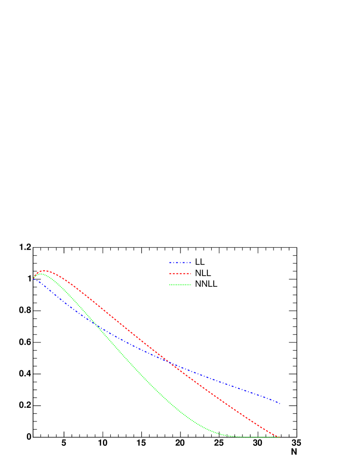
Figure 1: The moment–space Sudakov factor ${\rm Sud}(m,N)$, computed using Eq. (15) to LL, NLL and NNLL accuracy, plotted as dotdashes, dashes and dots, respectively. The curves end at $N\simeq 33$, corresponding to $\lambda=\frac{1}{2}$, where the Landau singularity in $g_{n}(\lambda)$ appears.

Fig. 1 shows the Sudakov factor of Eq. (15) with increasing logarithmic accuracy: $g_{0}(\lambda)$ only (LL accuracy), then $g_{0}(\lambda)$ and $g_{1}(\lambda)$ (NLL accuracy) and finally the first three terms (NNLL accuracy). We observe that the convergence of the series in Eq. (15) is poor. Non-negligible differences appear already in the first few moments. These will be partially washed out by matching the results with the fixed–order calculation. However, for $N\mathrel{\mathchoice{\vbox{\offinterlineskip\halign{$\m@th\displaystyle\hfil#\hfil$\cr>\crcr\sim\crcr} }}{\vbox{\offinterlineskip\halign{$\m@th\textstyle\hfil#\hfil$\cr>\crcr\sim\crcr} }}{\vbox{\offinterlineskip\halign{$\m@th\scriptstyle\hfil#\hfil$\cr>\crcr\sim\crcr} }}{\vbox{\offinterlineskip\halign{$\m@th\scriptscriptstyle\hfil#\hfil$\cr>\crcr\sim\crcr} }}}10$, where $\ln N$ starts to get large, the NNLL contribution of $g_{2}(\lambda)$ is already larger than that of the NLL term; for $N\mathrel{\mathchoice{\vbox{\offinterlineskip\halign{$\m@th\displaystyle\hfil#\hfil$\cr>\crcr\sim\crcr} }}{\vbox{\offinterlineskip\halign{$\m@th\textstyle\hfil#\hfil$\cr>\crcr\sim\crcr} }}{\vbox{\offinterlineskip\halign{$\m@th\scriptstyle\hfil#\hfil$\cr>\crcr\sim\crcr} }}{\vbox{\offinterlineskip\halign{$\m@th\scriptscriptstyle\hfil#\hfil$\cr>\crcr\sim\crcr} }}}18$ the NNLL contribution becomes larger than the leading-log term! This clearly indicates that the perturbative expansion breaks down. It is known from previous studies [19, 20, 21, 22, 16] that the asymptotic behavior of ${\rm Sud}(m,N)$ is controlled by infrared renormalons. In Ref. [16] it was shown, based on the resummation of running–coupling effects in the large–$\beta_{0}$ limit, that the expansion in Eq. (15) should break down early (see Fig. 2 there). Having at hand the full NNLL result we confirm that this is indeed so.

The conclusions are the following: first, it becomes obvious that the logarithmic accuracy criterion is, at best, insufficient. Moreover, since the poor convergence of the series in Eq. (15) is associated with running–coupling effects, these must be resummed. Finally, since the latter brings about infrared renormalon ambiguities that scale as powers of $(N\Lambda/m)$ the resolution of this problem is directly linked to the question of separation between perturbative and non-perturbative contributions: the calculation of the Sudakov exponent cannot be considered as a purely perturbative matter. Similar observations in different but analogous physics problems have led to the development of DGE [19, 20, 21, 22] as an alternative to resummation with fixed logarithmic accuracy.

Before moving on to DGE let us conclude our perturbative analysis by summarizing the state–of–the–art fixed–order and fixed–logarithmic–accuracy results. First, in Appendix A we derive explicit expressions for the log–enhanced terms at ${\cal O}(\alpha_{s}^{2})$. These will be useful for checking NNLO calculations. Finally, it is straightforward to invert the Mellin transform of ${\rm Sud}(m,N)$ in Eq. (15) to obtain a resummation formula with NNLL accuracy in $x$ space. The integrated spectrum with $E_{\gamma}>E_{0}=(1-\Delta)m/2$,

$$\Gamma[b\longrightarrow X_{s}\gamma]^{O_{7}}_{E_{\gamma}>E_{0}}(\Delta)\equiv\int_{1-\Delta}^{1}dx\,\frac{d\Gamma^{O_{7},\hbox{\tiny PT}}(x)}{dx},$$ (17)

is then:

$$\frac{\Gamma[b\longrightarrow X_{s}\gamma]^{O_{7}}_{E_{\gamma}>E_{0}}(\Delta)}{\Gamma_{\hbox{\tiny total}}^{O_{7},\hbox{\tiny PT}}}=C_{\infty}^{O_{7}}(\alpha_{s}(m))\frac{\exp\bigg{\{}g_{0}(\omega)\left(\frac{\alpha_{s}^{\hbox{\tiny${\overline{\rm MS}}$}}(m)}{\pi}\right)^{-1}+g_{1}(\omega)+g_{2}(\omega)\frac{\alpha_{s}^{\hbox{\tiny${\overline{\rm MS}}$}}(m)}{\pi}\bigg{\}}}{\Gamma\left(1-\beta_{0}\left(g_{0}^{\prime}(\omega)+g_{1}^{\prime}(\omega)\frac{\alpha_{s}^{\hbox{\tiny${\overline{\rm MS}}$}}(m)}{\pi}\right)\right)}$$

$$\hskip 12.0pt\times\left[1+\frac{1}{2}g_{0}^{\prime\prime}(\omega)\beta_{0}^{2}\frac{\alpha_{s}^{\hbox{\tiny${\overline{\rm MS}}$}}(m)}{\pi}\Big{(}\Psi^{2}\left(1-\beta_{0}g_{0}^{\prime}(\omega)\right)-\Psi^{\prime}\left(1-\beta_{0}g_{0}^{\prime}(\omega)\right)\Big{)}\right]\,+\,R_{O_{7}}(\Delta),$$ (18)

where

$$\omega\equiv\frac{\alpha_{s}^{\hbox{\tiny${\overline{\rm MS}}$}}(m^{2})}{\pi}\beta_{0}\ln\frac{1}{\Delta}.$$

Eq. (2.1) was matched to agree with the exact NLO expression upon expansion using Eq. (A):

$$C_{\infty}^{O_{7}}(\alpha_{s}(m))\simeq 1-C_{F}\,\frac{\alpha_{s}^{\hbox{\tiny${\overline{\rm MS}}$}}(m)}{\pi}\,\left(\frac{\gamma_{E}^{2}}{2}+\frac{\pi^{2}}{12}-\frac{7}{4}\gamma_{E}+\frac{31}{12}\right)+{\cal O}(\alpha_{s}^{2})$$ (19)

incorporates finite terms in the $N\longrightarrow\infty$ limit, while the additive contribution

$$R_{O_{7}}(\Delta)=\left[-\frac{1}{6}\Delta^{3}+\left(\frac{1}{4}\ln\Delta+\frac{1}{4}\right)\Delta^{2}+\left(\frac{5}{2}-\ln\Delta\right)\Delta\right]C_{F}\frac{\alpha_{s}^{\hbox{\tiny${\overline{\rm MS}}$}}(m)}{\pi}+{\cal O}(\alpha_{s}^{2})$$ (20)

completes the terms that vanish at $\Delta\longrightarrow 0$. Note that the currently unknown ${\cal O}(\alpha_{s}^{2})$ term in Eq. (19) influences NNLL terms in the spectrum (at ${\cal O}(\alpha_{s}^{3})$ and beyond) by mixing with the leading logarithms from the expansion of the exponential function in Eq. (2.1). Thus, although the Sudakov factor itself is known to NNLL accuracy, complete NNLL accuracy of the spectrum is not yet available.

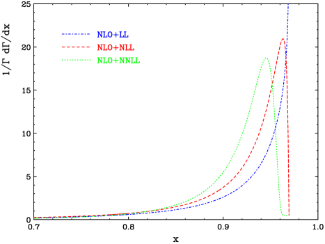
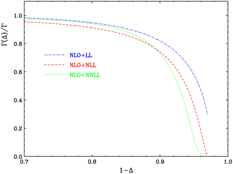
Figure 2: The differential (top) and the integrated (bottom) spectra based on the fixed–logarithmic–accuracy formula of Eq. (2.1), which is matched to NLO. The LL, NLL and NNLL accuracy results are plotted as dotdashes, dashes and dots, respectively. The three curves end at $x\simeq 0.97$, where the resummed results become complex owing to the Landau singularity at $\omega=1/2$.

The resulting spectrum with the Sudakov factor computed at NNLL accuracy is shown in Fig. 2 together with lower logarithmic accuracy results. We find that in spite of matching the resummed result to the NLO expression (this compensates for some of the difference observed in Fig. 1) differences between the three approximations to the spectrum are still large. Note that the three curves are not plotted beyond $x\simeq 0.97$, where Eq. (2.1) becomes complex owing to the presence of the Landau singularity at $\omega=1/2$. We observe that with increasing logarithmic accuracy the differential spectrum widens up and gets shifted to lower photon energies. While these features are intuitively expected, the instability of the perturbative result makes it hard to rely on this spectrum and use it as a baseline for parametrization of non-perturbative effects. An explicit separation criterion between the perturbative and non-perturbative regimes is clearly missing here. As we shall see below, these deficiencies are cured by DGE.

2.2 Borel representation of the exponent and the large–$\beta_{0}$ limit

According to Ref. [16] the Sudakov factor in Eq. (5) can be expressed as the following Borel sum:

$${\rm Sud}(m,N)\,\equiv\,\exp\bigg{\{}\frac{C_{F}}{\beta_{0}}\int_{0}^{\infty}\frac{du}{u}\,T(u)\,\left(\frac{\Lambda^{2}}{m^{2}}\right)^{u}\bigg{[}B_{\cal S}(u)\Gamma(-2u)\left(N^{2u}-1\right)-$$

$$\hskip 240.0ptB_{\cal J}(u)\Gamma(-u)\left(N^{u}-1\right)\bigg{]}\bigg{\}}.$$ (21)

Here we use the scheme–invariant Borel representation [33] where $T(u)$ is the Laplace transform of the ’t Hooft coupling:

$$A(\mu) = \frac{\beta_{0}\alpha_{s}^{\hbox{\tiny't Hooft}}(\mu)}{\pi}=\int_{0}^{\infty}{du}\,T(u)\,\left(\frac{\Lambda^{2}}{\mu^{2}}\right)^{u};\qquad\qquad\frac{dA}{d\ln\mu^{2}}=-A^{2}(1+\delta A),$$

$$T(u) = \frac{(u\delta)^{u\delta}{\rm e}^{-u\delta}}{\Gamma(1+u\delta)};\qquad\qquad\ln(\mu^{2}/\Lambda^{2})=\frac{1}{A}-\delta\ln\left(1+\frac{1}{\delta A}\right)$$ (22)

with $\delta\equiv\beta_{1}/\beta_{0}^{2}$, where the first two coefficients of the $\beta$ function are given in Eq. (13).

The functions $B_{\cal S}(u)$ and $B_{\cal J}(u)$ are the scheme invariant Borel representations of the anomalous dimensions of the soft (quark distribution) and the jet functions, respectively. Defining the Borel representation of the anomalous dimensions introduced in the previous section, namely

$${\cal A}\big{(}\alpha_{s}(\mu)\big{)}=\frac{C_{F}}{\beta_{0}}\int_{0}^{\infty}du\,T(u)\,\left(\frac{\Lambda^{2}}{\mu^{2}}\right)^{u}\,B_{\cal A}(u),$$

$${\cal B}\big{(}\alpha_{s}(\mu)\big{)}=\frac{C_{F}}{\beta_{0}}\int_{0}^{\infty}du\,T(u)\,\left(\frac{\Lambda^{2}}{\mu^{2}}\right)^{u}\,B_{\cal B}(u),$$

$${\cal D}\big{(}\alpha_{s}(\mu)\big{)}=\frac{C_{F}}{\beta_{0}}\int_{0}^{\infty}du\,T(u)\,\left(\frac{\Lambda^{2}}{\mu^{2}}\right)^{u}\,B_{\cal D}(u),$$ (23)

we have:

$$B_{\cal S}(u) = B_{\cal A}(u)-uB_{\cal D}(u),$$

$$B_{\cal J}(u) = B_{\cal A}(u)-uB_{\cal B}(u).$$ (24)

These are exact relations.

Using the perturbative expansions in Eqs. (2.1) through (11), one obtains the following expansions for the corresponding Borel functions at small $u$:

$$B_{\cal A}(u)=1+\left(\frac{5}{3}+c_{2}\right)\frac{u}{1!}+\left(-\frac{1}{3}+c_{3}\right)\frac{u^{2}}{2!}+\cdots,$$ (25)

where $c_{n}$ represent contributions that are subleading in $\beta_{0}$; $c_{2}$ and $c_{3}$ are (see Appendix C in [30]):

$$c_{2} = \frac{C_{A}}{\beta_{0}}\left(\frac{1}{3}-\frac{\pi^{2}}{12}\right)$$

$$c_{3} = \frac{1}{\beta_{0}}\left[\left(\frac{649}{288}-\frac{5}{18}\pi^{2}+\frac{7}{2}\zeta_{3}\right)C_{A}+\left(\frac{23}{8}-3\zeta_{3}\right)C_{F}\right]$$ (26)

$$+ \frac{1}{\beta_{0}^{2}}\left[\left(\frac{251}{288}+\frac{7}{144}\pi^{2}-\frac{11}{4}\zeta_{3}+\frac{11}{720}\pi^{4}\right)C_{A}^{2}+\left(-\frac{235}{96}+\frac{11}{4}\zeta_{3}+\frac{\pi^{2}}{16}\right)C_{F}C_{A}-\frac{3}{32}C_{F}^{2}\right]$$

$$+ \frac{1}{\beta_{0}^{3}}\left[\left(-\frac{301}{512}-\frac{7}{192}\pi^{2}\right)C_{A}^{3}+\left(-\frac{11}{64}-\frac{11}{192}\pi^{2}\right)C_{F}C_{A}^{2}+\frac{11}{128}C_{F}^{2}C_{A}\right].$$

and

$$B_{\cal D}(u) = 1+\left[\!{\displaystyle\frac{1}{9}}+{\displaystyle\frac{C_{A}}{{\beta_{0}}}{\left({\displaystyle\frac{9}{4}}\,\zeta_{3}-{\displaystyle\frac{\pi^{2}}{12}}-{\displaystyle\frac{11}{18}}\right)\,}}\!\right]u\,+\,{\cal O}(u^{2}),$$ (27)

$$B_{\cal B}(u) = -{\displaystyle\frac{3}{4}}+\left[{\displaystyle\frac{\pi^{2}}{6}}-{\displaystyle\frac{247}{72}}\,+\,{\displaystyle\frac{C_{A}}{\beta_{0}}{\left(-{\displaystyle\frac{73}{144}}+{\displaystyle\frac{5}{2}}\,\zeta_{3}\right)\,}}+{\displaystyle\frac{C_{F}}{\beta_{0}}{\left(-{\displaystyle\frac{3}{32}}-{\displaystyle\frac{3}{2}}\,\zeta_{3}+{\displaystyle\frac{\pi^{2}}{8}}\right)\,}}\right]u+{\cal O}(u^{2}).$$

Upon expanding the entire square brackets in Eq. (2.2) in powers of $u$ using Eqs. (2.2) through (27) one recovers the same log–enhanced terms presented in the previous section to NNLL accuracy. However, upon performing the Borel integral (barring renormalon singularities, see below) one can resum running–coupling effects to all orders. In the large–$\beta_{0}$ limit the Borel functions are given by [16, 22]:

$$B_{\cal S}(u) = {\rm e}^{\frac{5}{3}u}(1-u)\,+\,{\cal O}(1/\beta_{0}),$$

$$B_{\cal J}(u) = \frac{1}{2}\,{\rm e}^{\frac{5}{3}u}\left(\frac{1}{1-u}+\frac{1}{1-u/2}\right)\frac{\sin\pi u}{\pi u}\,+\,{\cal O}(1/\beta_{0}).$$ (28)

Note that these are entire functions, free of singularities in the whole complex plane. In the full theory, i.e. for finite $\beta_{0}$, analytic expressions of this kind are, of course, not known. In Sec. 2.3 we shall construct approximations to these unknown functions based on their small-$u$ expansions quoted above and some additional constraints. Because of the significant contribution of running–coupling effects [21, 20, 22, 16] the difference between performing the Borel integral (DGE) and extracting the leading logarithms to a fixed logarithmic accuracy is very significant. This will be explicitly demonstrated in the next section.

Writing the Sudakov factor of Eq. (2.2) in a factorized form, i.e.

$${\rm Sud}(m,N)=S_{N}(m;\mu)\,J_{N}(m;\mu),$$ (29)

requires subtraction of logarithmic singularities:

$$S_{N}(m;\mu)=\exp\bigg{\{}\frac{C_{F}}{\beta_{0}}\int_{0}^{\infty}\frac{du}{u}\,T(u)\,\left(\frac{\Lambda^{2}}{m^{2}}\right)^{u}\,\,\times$$ (30)

$$\hskip 130.0pt\bigg{[}B_{\cal S}(u)\Gamma(-2u)\left(N^{2u}-1\right)+\left(\frac{m^{2}}{\mu^{2}}\right)^{u}B_{\cal A}(u)\ln N\bigg{]}\bigg{\}},$$

$$J_{N}(m;\mu)=\exp\bigg{\{}-\frac{C_{F}}{\beta_{0}}\int_{0}^{\infty}\frac{du}{u}\,T(u)\,\left(\frac{\Lambda^{2}}{m^{2}}\right)^{u}\,\,\times$$ (31)

$$\hskip 130.0pt\bigg{[}B_{\cal J}(u)\Gamma(-u)\left(N^{u}-1\right)+\left(\frac{m^{2}}{\mu^{2}}\right)^{u}B_{\cal A}(u)\ln N\bigg{]}\bigg{\}},$$

where, as above, $B_{\cal A}(u)$ is the Borel representation of the cusp anomalous dimension. This anomalous dimension determines the factorization scale ($\mu$) dependence of the separate soft and the jet functions, while ${\rm Sud}(m,N)$ is independent of $\mu$:

$$\frac{d\ln S_{N}(m;\mu)}{d\ln\mu^{2}}=-\frac{d\ln J_{N}(m;\mu)}{d\ln\mu^{2}} \equiv -\frac{C_{F}}{\beta_{0}}{\cal A}(\alpha_{s}(\mu))\ln N.$$ (32)

Finally, note that the Sudakov factors Eq. (30) and Eq. (31) (and likewise Eq. (2.2)) have infrared renormalon singularities. As usual these singularities occur at integer (in both $J_{N}$ and $S_{N}$) and half integer (in $S_{N}$) values of the Borel variable $u$. To properly define these resummed Sudakov factors one needs to deform the integration contour off the real $u$ axis or take the Principal–Value prescription. We shall adopt the latter, which guaranties that ${\rm Sud}(m,N)$ is a real–valued function, namely

$${\rm Sud}(m,N)=\bigg{[}{\rm Sud}(m,N^{*})\bigg{]}^{*},$$ (33)

and, in particular, that it is real for real positive $N$, as it is at any finite order in perturbation theory. By choosing this prescription we have made an explicit separation between what will be regarded as resummed perturbation theory and additional non-perturbative power corrections, which we shall discuss in Sec. 4 below.

2.3 Renormalons beyond the large–$\beta_{0}$ limit

The all–order structure of the Sudakov exponent is summarized by Eq. (2.2). DGE makes use of this structure in spite of the limited knowledge of the functions $B_{\cal S}(u)$ and $B_{\cal J}(u)$. In the large–$\beta_{0}$ limit these functions, given by Eq. (2.2), are free of infrared renormalon singularities. Being anomalous dimensions they are expected to be free of renormalons also in the full theory. Similarly to other cases [19, 20, 21, 32, 22], infrared renormalons appearing in the Sudakov exponent (2.2) have a very specific origin: the integration over the longitudinal momentum fraction $z$ in the $z\longrightarrow 1$ limit. This integration gives rise to the factors $\Gamma(-2u)$ and $\Gamma(-u)$ in Eq. (30) and Eq. (31), respectively.

Eq. (30) therefore implies that the soft Sudakov exponent has simple renormalon poles at all integer and half integer values of $u$, except where $B_{\cal S}(u)$ vanishes. Similarly, according to Eq. (31), the jet function has simple renormalon poles at all integer values of $u$, except where $B_{\cal J}(u)$ vanishes. It turns out that in the large–$\beta_{0}$ limit these functions do vanish at some of the would-be renormalon positions: $B_{\cal S}(u)$ vanishes at $u=1$ while $B_{\cal J}(u)$ at all integers $u\geq 3$. It is not known whether the corresponding renormalons do appear in the full theory.

The theoretical interest aside, the renormalon structure of the Sudakov exponent, and in particular, that of the soft function, is important for phenomenology. Obviously, the most important renormalon singularity is the one at $u=\frac{1}{2}$. It has been shown in Ref. [16] that the associated ambiguity cancels out between the soft Sudakov exponent and the leading non-perturbative correction $\bar{\Lambda}=M-m$. For this cancellation to be realized — thus avoiding a spurious ${\cal O}(N\Lambda/m)$ artifact — both quantities need to be computed as asymptotic expansions, regularizing the $u=\frac{1}{2}$ renormalon in the same manner. As explained in the introduction, in this paper we shall implement this idea. We shall use the Cauchy Principal–Value prescription in the calculation of $\bar{\Lambda}$ from the ${\overline{\rm MS}}$ mass (see Sec. 4.2) and in the calculation of the Sudakov exponent.

Power accuracy is, however, not easy to achieve. The difficulty is that in order to accurately compute the Principal Value of the Borel integral, say in Eq. (30), the renormalon structure, including its overall normalization (the residue) must be known. Standard perturbative expansions of $B_{\cal S}(u)$ as in Eq. (27), yield power series in $u$, which may not be reliable near $u=\frac{1}{2}$. In the following we will address this problem. Higher renormalon singularities in the soft function scaling as higher powers of $N\Lambda/m$ are also relevant. One expects that these effects will mainly be important in the endpoint region. However, it is hard to know a priori how far from endpoint their influence extends. For the jet function the situation is different: the sensitivity to the functional form of $B_{\cal J}(u)$ away from the origin is small. This correspond to the fact that power corrections on the scale $m^{2}/N$ are smaller. In what follows we therefore concentrate on $B_{\cal S}(u)$ and, first of all, on its value at $u=\frac{1}{2}$ which determines the corresponding renormalon residue in Eq. (30) and in Eq. (2.2).

We first note that direct evaluation of the available NNLO expansion of $B_{\cal S}(u)$ at $u=\frac{1}{2}$ using Eq. (2.2) with Eqs. (25) and (27) is unreliable. The apparent convergence of the series (in the Borel plane) at the first three orders is slow: for example with $N_{f}=4$ the terms of increasing powers of $u$ are: $1$, $-0.0188$ and $-0.3415$. As the expansion of an anomalous dimension this series is expected to converge, but since the NNLO is sizable while the large–order behavior is not known, it appears that such a direct evaluation of the residue cannot be accurate.

Next, we note that the exact result of the large–$\beta_{0}$ limit, Eq. (2.2), constrains the anomalous dimensions to ${\cal O}(u^{0})$ only, and that the corrections to $B_{\cal S}(u)$ at ${\cal O}(u)$ and ${\cal O}(u^{2})$, which are subleading in $\beta_{0}$, are large. Thus, a naive non-Abelianization approach, in which ${\cal O}(1/\beta_{0})$ terms are neglected, is not sufficiently accurate. A similar conclusion was reached before [32] considering the case of the jet function.

Fortunately, indirect information on $B_{\cal S}(u)$ at $u=\frac{1}{2}$ is available owing to the exact cancellation [16] of the corresponding renormalon ambiguity with the one in $\bar{\Lambda}$, or in the pole mass. We note that the singularity structure of the $u=\frac{1}{2}$ renormalon in the pole mass [34] — a simple pole in the scheme invariant Borel function — matches exactly the one of the soft Sudakov exponent, as it should. As discussed in Appendix B, the normalization of the pole–mass renormalon at $\frac{1}{2}$ is well under control. This allows us to fix the value of the Borel function:

$$\left.B_{\cal S}(u)\right|_{u=\frac{1}{2}}=\frac{q}{2}{\rm e}^{\delta/2}.$$ (34)

The normalization constant $q$ — see Eq. (99) — has been computed from the perturbative relation between the pole mass and the ${\overline{\rm MS}}$ mass by several authors [35, 36, 37, 38], obtaining good numerical convergence already at the available NNLO. In Appendix B we summarize our own study of this renormalon. Previous work on the subject was restricted to the standard Borel representation and to the ${\overline{\rm MS}}$ scheme. We extend this analysis using the scheme–invariant formulation of the Borel transform. This provides an independent check of the accuracy of this calculation and facilitates the comparison with the Sudakov exponent.

The result for the normalization of the pole–mass renormalon at $\frac{1}{2}$ is shown in Fig. 13 in Appendix B. The close agreement between different calculational procedures based on the expansion of $m/m_{\hbox{\tiny${\overline{\rm MS}}$}}(m_{\hbox{\tiny${\overline{\rm MS}}$}})$ demonstrates the reliability of this determination. We conclude that the residue can be computed with $\sim 2-3\%$ accuracy over a wide range of $\beta_{0}$ values, in agreement with Refs. [35, 36, 37, 38]. As anticipated, the determination that relies on the soft Sudakov exponent is less accurate. Nevertheless, it does yield similar values.

As explained above, in order to evaluate the Sudakov exponent of Eq. (2.2) using the Principal–Value prescription we must know $B_{\cal S}(u)$ (and $B_{\cal J}(u)$) as a function of $u$ away from the origin. Any uncertainty would translate into uncertainty in the computed spectrum, and an ambiguity in the separation between perturbative and non-perturbative corrections. To gauge the numerical significance of this issue, let us construct a few models, which we generically call NNLL–DGE, that all share the same expansion in powers of $u$ up to the NNLO but differ away from the origin.

A natural possibility [19, 20, 22, 32] is to start with the analytic form of the large–$\beta_{0}$ limit, Eq. (2.2), and include a multiplicative correction factor that modifies the expansion coefficients at ${\cal O}(u)$ and at ${\cal O}(u^{2})$ by terms that are subleading in $\beta_{0}$, so as to match the exact coefficients given by Eq. (2.2) with Eq. (27).

At ${\cal O}(u)$ (NLL–DGE) this was already done in Ref. [16] following Refs. [19, 20, 21, 22] as follows:

$$B_{\cal S}^{\rm NLL-DGE}(u) = {\rm e}^{\left(\frac{5}{3}+c_{2}\right)u}(1-u)+\,{\cal O}(u^{2}),$$ (35)

and

$$B_{\cal J}^{\rm NLL-DGE}(u) = \frac{1}{2}\,{\rm e}^{\left(\frac{5}{3}+c_{2}\right)u}\left(\frac{1}{1-u}+\frac{1}{1-u/2}\right)\frac{\sin\pi u}{\pi u}\,+\,{\cal O}(u^{2}).$$ (36)

Proceeding to ${\cal O}(u^{2})$ (NNLL–DGE) one can write:

$$B_{\cal S}^{(a)}(u) = {\rm e}^{\frac{5}{3}u}(1-u)\,\times\,\exp{\bigg{\{}c_{2}u+\left[c_{3}-c_{2}^{2}+\frac{C_{A}}{\beta_{0}}\left(\frac{5}{18}\pi^{2}+\frac{7}{9}-\frac{9}{2}\zeta_{3}\right)\right]\frac{u^{2}}{2!}+{\cal O}(u^{3})\bigg{\}}},$$

$$B_{\cal J}^{(a)}(u) = \frac{1}{2}\,{\rm e}^{\frac{5}{3}u}\left(\frac{1}{1-u}+\frac{1}{1-u/2}\right)\frac{\sin\pi u}{\pi u}\,\times$$

$$\exp{\bigg{\{}c_{2}u+\left[c_{3}-c_{2}^{2}+\frac{C_{A}}{\beta_{0}}\left(\frac{29}{72}\pi^{2}-\frac{43}{72}-5\zeta_{3}\right)+\frac{C_{F}}{\beta_{0}}\left(-\frac{\pi^{2}}{4}+\frac{3}{16}+3\zeta_{3}\right)\right]\frac{u^{2}}{2!}+{\cal O}(u^{3})\bigg{\}}}.$$

It is straightforward to check that the this model coincides with the exact analytic functions in the large–$\beta_{0}$ limit on the one hand, and has the exact expansion coefficients to the NNLO on the other.

Let us recall that a similar exercise has already been done for the jet function in Ref. [32], in the context of the large–$x$ limit of deep inelastic structure functions. Since in the case of decay spectra the soft function plays a dominant role, we shall adopt the model of Eq. (2.3) for $B_{\cal J}(u)$ and not consider here other possibilities.

An alternative model for the soft function is given by

$$B_{\cal S}^{(b)}(u)={\rm e}^{\frac{5}{3}u}(1-u)\,\times\,\bigg{\{}1+c_{2}u+\left[c_{3}+\frac{C_{A}}{\beta_{0}}\left(\frac{5}{18}\pi^{2}+\frac{7}{9}-\frac{9}{2}\zeta_{3}\right)\right]\frac{u^{2}}{2!}+{\cal O}(u^{3})\bigg{\}}.$$ (38)

The main difference between $B_{\cal S}^{(a)}(u)$ and $B_{\cal S}^{(b)}(u)$ is that the former inherently suppresses contributions from the large–$u$ region, which is, in any case, not well controlled. While in general the large–$u$ region is suppressed in the Borel integral (2.2) by $(\Lambda^{2}/m^{2})^{u}$, at large $N$ this is replaced by $(N^{2}\Lambda^{2}/m^{2})^{u}$. This suppression is relevant up to $N\sim m/\Lambda$. Beyond this region the Borel integral still converges thanks to the suppression by the factor $\Gamma(-2u)$, however, the perturbative result is no more a valid approximation; the power expansion breaks down.

Figure 3: Top: the Borel representation of the soft anomalous dimension, $B_{\cal S}(u)$, as a function of $u$ for $N_{f}=4$. Vertical lines indicate potential renormalon locations. Bottom: Contributions to the Principal–Value integral over $u$ in the Sudakov exponent of Eq. (2.2) for $N=20$ from the corresponding sections, each containing one renormalon (or none). In each figure the five curves corresponds to the different models described in the text: NLL–DGE as thin full line and NNLL–DGE: ($a$) as dotdashes, ($b$) as dashes, ($c$) as thick full line, and ($d$) as dots.

For $N\mathrel{\mathchoice{\vbox{\offinterlineskip\halign{$\m@th\displaystyle\hfil#\hfil$\cr<\crcr\sim\crcr} }}{\vbox{\offinterlineskip\halign{$\m@th\textstyle\hfil#\hfil$\cr<\crcr\sim\crcr} }}{\vbox{\offinterlineskip\halign{$\m@th\scriptstyle\hfil#\hfil$\cr<\crcr\sim\crcr} }}{\vbox{\offinterlineskip\halign{$\m@th\scriptscriptstyle\hfil#\hfil$\cr<\crcr\sim\crcr} }}}m/\Lambda$ the perturbative calculation by DGE is under control. Nevertheless, non-negligible contributions may still arise from the vicinity of the renormalon positions where the factor $\Gamma(-2u)$ is singular. These are power suppressed terms. Indeed, looking in Fig. 3 at the contributions to the Sudakov exponent from different sections along the Borel integration axis for $N=20$, models $(a)$ and $(b)$ appear rather different: while model $(a)$ is characterized by very small contributions beyond $u\sim 1.5$, in model $(b)$ these are not small up to $u$ of a few tens. This directly reflects the (exponential) suppression of the large–$u$ region in $B_{\cal S}^{(a)}(u)$ versus its enhancement in $B_{\cal S}^{(b)}(u)$. We note, however, that the NLL–DGE model of Eq. (35) does not generate significant contributions from $u$ values beyond $u\sim 1.5$, although it has no inherent exponential suppression of the large–$u$ region.

To draw conclusions with regards to the net effect of the behavior of the models for $B_{\cal S}(u)$ away from the origin we now examine the value of the Sudakov factor ${\rm Sud}(m,N)$ of Eq. (2.2). The result, shown in Fig. 4, is clear: models $(a)$ and $(b)$ as well as the NLL–DGE one are close up to very high moments. This means that the total effect of the large–$u$ region of $B_{\cal S}(u)$, which is not under control, is moderate; in model $(b)$ this is owing to cancellations between contributions from the different sections in Fig. 3. On the whole the DGE result is stable. Nevertheless, the differences between the models are non-negligible.

Fig. 4 also shows that some difference between DGE and the conventional Sudakov–resummation procedure (with NNLL accuracy) develops already at low moments $N<10$, and that it becomes very significant for $N\sim 10-20$. One qualitative difference is that the latter has a Landau singularity ($N\simeq 33$) whereas the former does not [22].

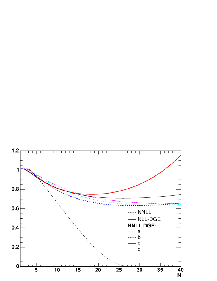
Figure 4: The moment–space Sudakov factor ${\rm Sud}(m,N)$, as computed by DGE with perturbative expansions of NLL and NNLL accuracy (in the latter case the four models $(a)$ through $(d)$ are shown) and by conventional Sudakov resummation with NNLL accuracy.

A shortcoming of the models constructed so far is that they are inaccurate around $u=\frac{1}{2}$: Eq. (34) is not fulfilled. In order to incorporate the knowledge of $B_{\cal S}(u)$ at $u=\frac{1}{2}$ we consider the following model:

$$B_{\cal S}^{(c)}(u) = {\rm e}^{\frac{5}{3}u}(1-u)\,\times\,\exp\left\{c_{2}u+\frac{1}{2}\left[c_{3}-c_{2}^{2}+\frac{C_{A}}{\beta_{0}}\left(\frac{5}{18}\pi^{2}+\frac{7}{9}-\frac{9}{2}\zeta_{3}\right)\right]u^{2}\right\}\times W(u),$$

which, similarly to models $(a)$ and $(b)$, has the exact coefficients through ${\cal O}(u^{2})$ and the correct large–$\beta_{0}$ limit. Here, however, the additional factor

$$W(u)\equiv{\rm e}^{w_{1}u+\frac{1}{2}w_{2}u^{2}}\,\left(1-w_{1}u+\frac{1}{2}(w_{1}^{2}-w_{2})u^{2}\right)=1+{\cal O}(u^{3}),$$

is constructed such that correct value of $B_{\cal S}(u)$ at $u=\frac{1}{2}$ would be reproduced, at least for the physically relevant values of $N_{f}$. To this end we set:

$$\begin{array}[]{ll}w_{1}=1.144C_{A}/\beta_{0},&\hskip 20.0ptw_{2}=-2.8C_{A}/\beta_{0}.\end{array}$$ (41)

The values of $B_{\cal S}(u)$ at $u=\frac{1}{2}$ in the different models are shown as a function of $1/\beta_{0}$ in Fig. 5.

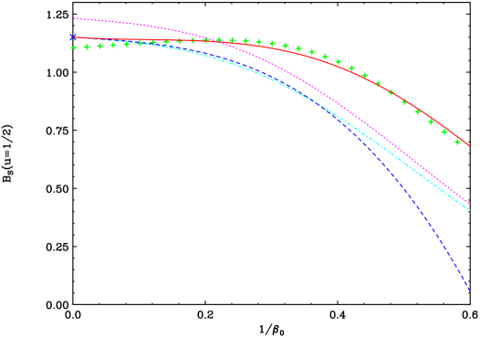
Figure 5: The value of the Borel representation of the soft anomalous dimension $B_{\cal S}(u)$ at $u=\frac{1}{2}$, which is proportional to the residue of the $u=\frac{1}{2}$ renormalon in the pole mass, plotted as a function of $1/\beta_{0}$. The exact result of the large–$\beta_{0}$ limit is denoted by a cross. The calculation relying on perturbative expansion of $m/m_{\hbox{\tiny${\overline{\rm MS}}$}}(m_{\hbox{\tiny${\overline{\rm MS}}$}})$ using the scheme–invariant Borel transform as determined using Eq. (113) is shown by plus signs. The four curves corresponds to the different models for NNLL–DGE described above: ($a$) dotdashes, ($b$) dashes, ($c$) full line and ($d$) dots. Model $(c)$ matches the computed value of $B_{\cal S}(u=\frac{1}{2})$ at $N_{f}=4$ by construction.

Returning to Fig. 4, we observe that fixing the value at $u=\frac{1}{2}$ makes a large effect on high moments $N\mathrel{\mathchoice{\vbox{\offinterlineskip\halign{$\m@th\displaystyle\hfil#\hfil$\cr>\crcr\sim\crcr} }}{\vbox{\offinterlineskip\halign{$\m@th\textstyle\hfil#\hfil$\cr>\crcr\sim\crcr} }}{\vbox{\offinterlineskip\halign{$\m@th\scriptstyle\hfil#\hfil$\cr>\crcr\sim\crcr} }}{\vbox{\offinterlineskip\halign{$\m@th\scriptscriptstyle\hfil#\hfil$\cr>\crcr\sim\crcr} }}}20$. This shows that this information is relevant for the final spectrum. Nevertheless, the fact that differences with the other models are moderate for $N\mathrel{\mathchoice{\vbox{\offinterlineskip\halign{$\m@th\displaystyle\hfil#\hfil$\cr<\crcr\sim\crcr} }}{\vbox{\offinterlineskip\halign{$\m@th\textstyle\hfil#\hfil$\cr<\crcr\sim\crcr} }}{\vbox{\offinterlineskip\halign{$\m@th\scriptstyle\hfil#\hfil$\cr<\crcr\sim\crcr} }}{\vbox{\offinterlineskip\halign{$\m@th\scriptscriptstyle\hfil#\hfil$\cr<\crcr\sim\crcr} }}}20$ is reassuring.

Finally, let us focus on the peculiar feature of the large–$\beta_{0}$ result for $B_{\cal S}(u)$, namely its vanishing at $u=1$, leading to the absence of a corresponding renormalon ambiguity. In the models considered so far we assumed that this property is shared by the full theory. This, however, has not been proven. Moreover, in Ref. [43] it has been shown that a $u=1$ renormalon appears in the kinetic–energy operator once terms that are subleading in $1/\beta_{0}$ are taken into account. This suggest that the same might occur in the Sudakov exponent, although this should be checked explicitly. In order to estimate the numerical significance of this issue, let us construct another model, $(d)$, which has $B_{\cal S}^{(d)}(u=1)\neq 0$:

$$B_{\cal S}^{(d)}(u) = \exp\left\{\left(\frac{2}{3}+c_{2}\right)u+\frac{1}{2}\left[c_{3}-c_{2}^{2}+\frac{C_{A}}{\beta_{0}}\left(\frac{5}{18}\pi^{2}+\frac{7}{9}-\frac{9}{2}\zeta_{3}\right)-1\right]u^{2}\right\}.$$ (42)

While $B_{\cal S}^{(d)}(u)$ does not respect the large–$\beta_{0}$ limit result, it does have the correct NNLO expansion at $u=0$. Returning again to Fig. 4, we observe that the effect of this modification is moderate, although probably not negligible.

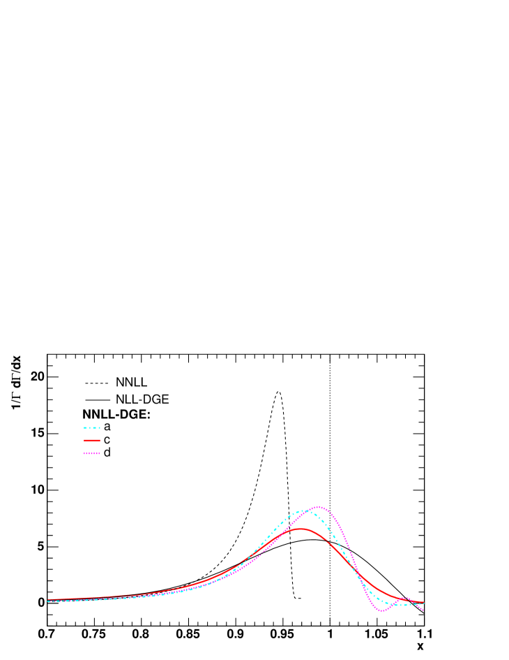
Figure 6: The perturbative differential spectrum in $b\longrightarrow X_{s}\gamma$ with different approximations for the Sudakov factor as a function of $x=2E_{\gamma}/m$, normalized by the total rate with $E_{\gamma}>m/20$. The different curves correspond to conventional Sudakov resummation with NNLL accuracy (thin dashed line) and DGE with perturbative expansions of NLL (thin full line) and NNLL accuracy (thick lines) where the three models $(a)$, $(c)$ and $(d)$ are shown by dotdashed, full and dotted lines, respectively.

Finally, let us compare between the different calculations of the resummed Sudakov exponent described above at the level of the normalized differential spectrum. To this end we match the resummed expression for the Sudakov factor with the full NLO result as explained in Sec. 3 below. Both the Borel integration in the Sudakov exponent in Eq. (2.2) and the inverse–Mellin integration in Eq. (6) are performed numerically, avoiding any further approximation. The results are shown in Fig. 6. Using DGE, the differences between different models with NLL or NNLL accuracy are moderate. On the other hand the result obtained by conventional NNLL Sudakov resummation is entirely different in spite of having the same formal logarithmic accuracy!

It is interesting to note that the DGE result does not have the perturbative support properties: while the perturbative coefficients at any given order vanish for $E_{\gamma}>m/2$, the DGE–resummed spectrum does not. It peaks for $E_{\gamma}\mathrel{\mathchoice{\vbox{\offinterlineskip\halign{$\m@th\displaystyle\hfil#\hfil$\cr<\crcr\sim\crcr} }}{\vbox{\offinterlineskip\halign{$\m@th\textstyle\hfil#\hfil$\cr<\crcr\sim\crcr} }}{\vbox{\offinterlineskip\halign{$\m@th\scriptstyle\hfil#\hfil$\cr<\crcr\sim\crcr} }}{\vbox{\offinterlineskip\halign{$\m@th\scriptscriptstyle\hfil#\hfil$\cr<\crcr\sim\crcr} }}}m/2$ and then smoothly crosses the perturbative endpoint $E_{\gamma}=m/2$ and drops to zero at $E_{\gamma}=\left(m+{\cal O}(\Lambda)\right)/2$. The resummed expression having different analytic properties than the coefficients is not surprising given that, strictly speaking, the sum does not exist. Nevertheless, it is remarkable that by taking the Principal–Value prescription in moment space we obtain a spectrum, which qualitatively corresponds to the decay of a higher–mass state.

3 Matching the resummed spectrum to the full NLO result

In the previous section we discussed the QCD description of the endpoint region neglecting ${\cal O}(1/N)$ corrections. In order to recover the correct spectrum away from the endpoint region, the resummed result must be systematically matched onto the fixed–order perturbative expansion, which is available in full at NLO — see Refs. [45, 47, 46] and references therein.

3.1 The NLO result

The NLO calculation in the Standard Model is based on the effective Hamiltonian

$${\cal H}_{\hbox{\tiny eff}}=\frac{4G_{F}}{\sqrt{2}}V^{*}_{ts}V_{tb}\sum_{k=1}^{8}C_{k}O_{k}$$ (43)

where $C_{k}$ are the Wilson coefficients and $O_{k}$ are local operators of dimension 5 or 6. The most important operator contributing at leading order corresponds to the magnetic interaction,

$$O_{7}=\frac{e\,m_{\hbox{\tiny${\overline{\rm MS}}$}}}{16\pi^{2}}\,\left(\bar{s}_{L}\sigma^{\mu\nu}b_{R}\right)\,F_{\mu\nu},$$ (44)

where $m_{\hbox{\tiny${\overline{\rm MS}}$}}$ is the running quark mass in the $\overline{\rm MS}$ scheme and $F_{\mu\nu}$ is the photon field strength. The complete basis of operators can be found for example in Refs. [45, 47].

Sudakov logarithms originate in the universal soft and collinear limits in which the specific structure of the hard interaction is irrelevant. Therefore, the calculation in Ref. [16] and the formulae of the previous section, although derived starting with $O_{7}$, apply to all operators. Terms that are finite (or vanish) at large $N$, e.g. those of Eq. (A), are different between the different operators. These terms will now be incorporated in the process of matching the Sudakov exponent to the full NLO result.

Our treatment of the endpoint region is based on moment space. On the other hand contributions that are non-singular at $x=1$ may be included either in moment space or directly in $x$ space. Since $b\longrightarrow s\gamma g$ contributions associated with $O_{8}$ are singular at $x\longrightarrow 0$ (when the photon gets soft) full NLO analysis in moment space is excluded. We therefore choose a mixed matching procedure where the dominant contribution at large $x$ is taken into account in moment space, but some terms, which vanish at $x\longrightarrow 1$, are included directly in $x$ space.

Let us express the partonic decay rate with photon energy above some fixed energy cut $E_{0}=(1-\Delta){m}/{2}$ as:

$$\Gamma[b\longrightarrow X_{s}\gamma]_{E_{\gamma}>E_{0}}=\Gamma_{\hbox{\tiny LO}}\times\bigg{[}|{\cal M}_{V}|^{2}\,\theta(\Delta>0)+R(\Delta)\bigg{]},$$ (45)

where $\theta(\Delta>0)$ is the heaviside function and

$$\Gamma_{\hbox{\tiny LO}} = \frac{G_{F}^{2}m^{3}m_{\hbox{\tiny${\overline{\rm MS}}$}}^{2}(m)}{32\pi^{4}}\left|V_{ts}^{*}V_{tb}\right|^{2}\left(C_{7}^{(0)\,eff}(\mu_{b})\right)^{2},$$ (46)

where $m\equiv m_{b}$, the b-quark pole mass, $m_{\hbox{\tiny${\overline{\rm MS}}$}}(m)$ is the running mass evaluated at $m$ and, finally, $\mu_{b}\simeq m$. In Eq. (45) ${\cal M}_{V}$ corresponds to the amplitude of the process $b\longrightarrow s\gamma$ so it begins at ${\cal O}(\alpha_{s}^{0})$ and includes all the purely virtual corrections at higher orders, while $R(\Delta)$ corresponds to partonic processes with at least one gluon in the final state, and it therefore begins at ${\cal O}(\alpha_{s})$ and depends on $\Delta$. At NLO one has [45]:

$${\cal M}_{V} = 1\,+\,\frac{\alpha_{s}}{4\pi}\left(\frac{C_{7}^{(1)\,\hbox{\tiny eff}}(\mu_{b})}{C_{7}^{(0)\,\hbox{\tiny eff}}(\mu_{b})}+\!\!\sum_{i=1..8}\frac{C_{i}^{(0)\,\hbox{\tiny eff}}(\mu_{b})}{C_{7}^{(0)\,\hbox{\tiny eff}}(\mu_{b})}\left[r_{i}+\gamma_{i7}^{(0)\,\hbox{\tiny eff}}\ln\frac{m}{\mu_{b}}\right]\right)+\cdots$$

$$R(\Delta) = \frac{C_{F}\alpha_{s}}{\pi}\Bigg{(}-\frac{1}{2}\ln^{2}\Delta-\frac{7}{4}\ln\Delta\,+\!\!\sum_{\scriptsize\begin{array}[]{c}{i,j=1..8}\\ {i\leq j}\end{array}}c_{ij}\,\phi_{ij}(\Delta)\Bigg{)}+\cdots,$$ (49)

where

$$c_{ij}\equiv\frac{C_{i}^{(0)\,\hbox{\tiny eff}}(\mu_{b})C_{j}^{(0)\,\hbox{\tiny eff}}(\mu_{b})}{\left(C_{7}^{(0)\,\hbox{\tiny eff}}(\mu_{b})\right)^{2}}.$$

The expressions for the LO coefficients $C_{i}^{(0)\,\hbox{\tiny eff}}$, the NLO coefficients $C_{i}^{(1)\,\hbox{\tiny eff}}$ and the (complex) constants $r_{i}$ as well as the anomalous dimensions $\gamma_{i7}^{(0)\,\hbox{\tiny eff}}$ can be found e.g. in [45, 44]. In $R(\Delta)$ we exhibited explicitly the terms that are singular at the phase–space boundary $\Delta\longrightarrow 0$ (or $x\longrightarrow 1$). These terms must be resummed to all orders incorporating the cancellation of divergences between real emission and virtual corrections. All the functions $\phi_{ij}(\Delta)$ vanish at $\Delta=0$ — see Appendix C for explicit expressions.

3.2 The matching procedure

Our goal is to improve the determination of $\Gamma[b\longrightarrow X_{s}\gamma]_{E_{\gamma}>E_{0}=(1-\Delta){m}/{2}}$ in Eq. (45) for small values of $\Delta$ by performing Sudakov resummation. At the same time we require that upon expansion the matched expression would coincide with the fixed–order result for any $\Delta$. To perform the matching we first split the real–emission terms into two parts, writing

$$\frac{1}{\Gamma_{\hbox{\tiny LO}}}\Gamma[b\longrightarrow X_{s}\gamma]_{E_{\gamma}>E_{0}=xm/2}=|{\cal M}_{V}|^{2}\,\bigg{[}\theta(x<1)+G_{1}(x)\bigg{]}\,+\,G_{2}(x),$$ (50)

where both $G_{1,2}(x)$ begin at ${\cal O}(\alpha_{s})$ and we require that $G_{1}(x)$ contains all the singular terms for $x\longrightarrow 1$ whereas $G_{2}(x)={\cal O}((1-x)^{2})$ so that it does not contribute to the differential rate near $x=1$:

$$\frac{1}{\Gamma_{\hbox{\tiny LO}}}\,\frac{d\Gamma^{\hbox{\tiny PT}}(x)}{dx}=|{\cal M}_{V}|^{2}\left[\delta(1-x)-\frac{dG_{1}(x)}{dx}\right]-\frac{dG_{2}(x)}{dx}.$$ (51)

Finally, we replace the square brackets by a matched Sudakov resummation (or DGE) formula in moment space while the $G_{2}$ term is left in $x$ space,

$$\frac{1}{\Gamma_{\hbox{\tiny LO}}}\,\frac{d\Gamma^{\hbox{\tiny PT}}(x)}{dx}=|{\cal M}_{V}|^{2}\int_{c-i\infty}^{c+i\infty}\frac{dN}{2\pi i}x^{-N}M_{N}^{\hbox{\tiny PT}}-\frac{dG_{2}(x)}{dx},$$ (52)

where $M_{N}^{\hbox{\tiny PT}}$ is proportional to the Sudakov factor ${\rm Sud}(N)$ in Eq. (2.2). Here we used the inverse Mellin transform formula of Eq. (6).

Eq. (52) is, by construction, consistent with both the fixed–order expansion and the resummed expression in the $x\longrightarrow 1$ limit. From Eqs. (50), (51) and (52) it follows that

$$M_{N}^{\hbox{\tiny PT}}=1+G_{1}(x=0)-\int_{0}^{1}dxx^{N-1}\left\{\frac{dG_{1}(x)}{dx}\right\}_{+},$$ (53)

where $\{\,\,\}_{+}$ stand for the “+” prescription (see Eq. (91)). Note that the contribution to the $N=1$ moment from the integral vanishes, so $M_{N=1}=1+G_{1}(x=0)$. We emphasize that, in contrast with our definition of $\bar{M}_{N}$ in Sec. 2, $M_{N=1}\neq 1$: the distribution is not normalized.

3.3 Matching formulae at NLO

This matching procedure can be applied at any order. Specifically, at NLO we have:

$$G_{1}(x) = \frac{C_{F}\alpha_{s}}{\pi}\Bigg{(}-\frac{1}{2}\ln^{2}(1-x)-\frac{7}{4}\ln(1-x)+\!\!\!\sum_{\scriptsize\begin{array}[]{c}{i,j=1..8}\\ {i\leq j}\end{array}}\!\!\!c_{ij}\,\eta_{ij}(\Delta=1-x)\Bigg{)}+{\cal O}(\alpha_{s}^{2}),$$ (55)

$$G_{2}(x) = \frac{C_{F}\alpha_{s}}{\pi}\sum_{\scriptsize\begin{array}[]{c}{i,j=1..8}\\ {i\leq j}\end{array}}c_{ij}\,\xi_{ij}(\Delta=1-x)+{\cal O}(\alpha_{s}^{2}),$$ (58)

where $\phi_{ij}(\Delta)=\eta_{ij}(\Delta)+\xi_{ij}(\Delta)$ with $\xi_{ij}(\Delta)={\cal O}(\Delta^{2})$; the explicit expressions for $\eta_{ij}$ and $\xi_{ij}$ appear in Appendix C. Using Eq. (53) with Eq. (55) we then get:

$$M_{N}^{\hbox{\tiny PT}} = 1+\frac{C_{F}\alpha_{s}}{\pi}\Bigg{\{}\int_{0}^{1}dxx^{N-1}\Bigg{[}-\frac{\ln(1-x)}{1-x}-\frac{7}{4}\frac{1}{1-x}+\!\!\sum_{\scriptsize\begin{array}[]{c}{i,j=1..8}\\ {i\leq j}\end{array}}\!\!\!c_{ij}\,\left.\frac{d\eta_{ij}(\Delta)}{d\Delta}\right|_{\Delta=1-x}\Bigg{]}_{+}$$

$$\hskip 60.0pt+\sum_{\scriptsize\begin{array}[]{c}{i,j=1..8}\\ {i\leq j}\end{array}}\!\!\!c_{ij}\,\eta_{ij}(\Delta=1)\Bigg{\}}\,+\,{\cal O}(\alpha_{s}^{2})$$

Performing the $x$-integration and extracting the single and double $\ln N$ terms which are included in the Sudakov exponent we finally obtain the matched Sudakov–resummed moments:

$$M_{N}^{\hbox{\tiny PT}}=\Bigg{[}1+\frac{C_{F}\alpha_{s}}{\pi}\Bigg{(}f(N)+\!\!\sum_{\scriptsize\begin{array}[]{c}{i,j=1..8}\\ {i\leq j}\end{array}}c_{ij}\,\mu_{ij}(N)\Bigg{)}\Bigg{]}\,\times\,{\rm Sud}(m,N),$$ (61)

where

$$f(N)=-\frac{1}{2}(\Psi(N)+\gamma_{E})^{2}+\frac{1}{2}\Psi_{1}(N)-\frac{\pi^{2}}{12}+\frac{7}{4}(\Psi(N)+\gamma_{E})+\frac{1}{2}\ln^{2}N-\left(\frac{7}{4}-\gamma_{E}\right)\ln N$$

and

$$\mu_{ij}(N)\equiv\int_{0}^{1}dxx^{N-1}\left.\frac{d\eta_{ij}(\Delta)}{d\Delta}\right|_{\Delta=1-x}.$$ (62)

It is straightforward to verify that, upon expanding Eq. (61) to ${\cal O}(\alpha_{s})$, Eq. (52) reproduces the full NLO result. The $x\longrightarrow 1$ singular terms in $-\frac{dG_{1}(x)}{dx}$ are taken into account through the Sudakov factor: they coincide with the ${\cal O}(\alpha_{s})$ terms in Eq. (A); the finite terms are incorporated into $M_{N}^{\hbox{\tiny PT}}$, and the remaining terms, which vanish at $x=1$, appear explicitly in $-\frac{dG_{2}(x)}{dx}$.

The explicit expressions for $\mu_{ij}(N)$ appear in Appendix C. Having extracted the factor $|{\cal M}_{V}|^{2}$ which contains the constants at ${\cal O}(\alpha_{s})$ in Eq. (52), $\mu_{ij}(N)$ vanish at large $N$ and the information needed to compute the ${\cal O}(\alpha_{s}^{2}\,\ln N)$ term in $M_{N}^{\hbox{\tiny PT}}$ is fully contained in $f(N)$ and the NNLL contributions to the exponent in ${\rm Sud}(m,N)$.

Having matched the result at NLO only, non-singular terms at ${\cal O}(\alpha_{s}^{2})$ are not under control. These terms depend on the details of the matching procedure. The particular choice we made gives preference to the moment–space treatment: as reflected in Fig. 7 the contribution of $G_{2}$ is very small.

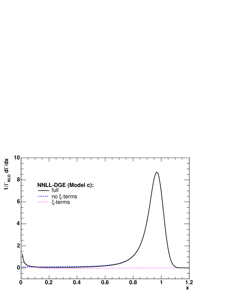
Figure 7: The differential spectrum according to Eq. (65) with $M_{N}^{\hbox{\tiny PT}}$ computed by NNLL–DGE using Eq. (61) (where the Sudakov factor is evaluated by Eq. (2.2) using model ($c$) of Eq. (2.3)). We show the spectrum matched to the full NLO result (full line) together with the separate contributions in Eq. (65) that are taken into account in moment space (dashed line) and in $x$ space (dotted line), respectively. The latter is significant only for $x\longrightarrow 0$.

To conclude this section we summarize the result. The Sudakov–resummed differential rate, matched to the exact NLO result, takes the form:

$$\frac{1}{\Gamma_{\hbox{\tiny NLO}}}\,\frac{d\Gamma^{\hbox{\tiny PT}}(x)}{dx}=\int_{c-i\infty}^{c+i\infty}\frac{dN}{2\pi i}x^{-N}M_{N}^{\hbox{\tiny PT}}+\frac{C_{F}\alpha_{s}(m_{b})}{\pi}\!\!\sum_{\scriptsize\begin{array}[]{c}{i,j=1..8}\\ {i\leq j}\end{array}}\!\!\!c_{ij}\,\left.\frac{d\xi_{ij}(\Delta)}{d\Delta}\right|_{\Delta=1-x}$$ (65)

where the moments $M_{N}^{\hbox{\tiny PT}}$ are given by Eq. (61) and the normalization is fixed by $\Gamma_{\hbox{\tiny NLO}}$, which is defined such that:

$$\Gamma[b\longrightarrow X_{s}\gamma]_{E_{\gamma}>E_{0}=(1-\Delta){m}/{2}}=\Gamma_{\hbox{\tiny NLO}}\times\left[\theta(\Delta>0)+R(\Delta)\right],$$

$${\rm with}$$

$$\Gamma_{\hbox{\tiny NLO}} = \frac{G_{F}^{2}m^{3}m_{\hbox{\tiny${\overline{\rm MS}}$}}^{2}(m)}{32\pi^{4}}\left|V_{ts}^{*}V_{tb}\right|^{2}\left(C_{7\gamma}^{\hbox{\tiny eff}}(\mu_{b})\right)^{2}\,\times$$

$$\hskip 100.0pt\left\{1+\frac{\alpha_{s}}{2\pi}\sum_{i=1..8}\frac{C_{i}^{(0)\,\hbox{\tiny eff}}(\mu_{b})}{C_{7}^{(0)\,\hbox{\tiny eff}}(\mu_{b})}\left[{\rm Re}\{r_{i}\}+\gamma_{i7}^{(0)\,\hbox{\tiny eff}}\ln\frac{m}{\mu_{b}}\right]\right\},$$

where $C_{7\gamma}^{\hbox{\tiny eff}}(\mu_{b})=C_{7}^{(0)\,\hbox{\tiny eff}}(\mu_{b})+\frac{\alpha_{s}}{4\pi}C_{7}^{(1)\,\hbox{\tiny eff}}(\mu_{b})$. We emphasize that the contribution of the $\xi_{ij}$ terms, which is treated in $x$ space, vanishes linearly with $(1-x)$ at large $x$ and it is numerically very small in the experimentally relevant region of $x$.

Finally, the corresponding formula for the total rate with an energy cut $E_{\gamma}>E_{0}=(1-\Delta){m}/{2}$ is:

$$\frac{1}{\Gamma_{\hbox{\tiny NLO}}}\Gamma[b\longrightarrow X_{s}\gamma]_{E_{\gamma}>E_{0}}\!=\!\!\int_{c-i\infty}^{c+i\infty}\frac{dN}{2\pi i}\,\frac{(1-\Delta)^{1-N}}{N-1}M_{N}^{\hbox{\tiny PT}}\!+\!\frac{C_{F}\alpha_{s}(m_{b})}{\pi}\!\!\!\!\!\!\!\sum_{\scriptsize\begin{array}[]{c}{i,j=1..8}\\ {i\leq j}\end{array}}\!\!\!\!\!c_{ij}\xi_{ij}(\Delta),$$ (69)

where $c>1$. Note that at $\Delta\longrightarrow 1$ (completely inclusive measurement) the inverse Mellin integral in Eq. (69) becomes trivial: it equals $M_{N=1}$.

4 Power corrections

The perturbative analysis of decay spectra in the endpoint region [4, 16] exposes the presence of three different scales: (1) hard, corresponding to virtual corrections with momenta ${\cal O}(m)$; (2) final–state dynamics of the jet with invariant mass squared ${\cal O}(m^{2}/N)$; and (3) soft radiation, with momenta ${\cal O}(m/N)$, that determines the heavy–quark momentum distribution function. Naturally, there is also non-perturbative dynamics on each of these scales, which brings about power corrections. The largest power corrections are clearly those on the soft scale. Smaller power corrections, which nevertheless become increasingly important near the endpoint, are the ones corresponding to the jet–mass scale. Their combined effect is related to the appearance of resonances when the jet mass is sufficiently small. In the following we address power corrections on the soft scale only.

4.1 Power corrections on the soft scale

The classical approach to the quark distribution function [1, 2] is based on the OPE. Expanding the non-local lightcone operator in Eq. (1) in powers of the lightcone separation $y^{-}$ one obtains local operators with a corresponding number of $iD_{+}$ derivatives. The matrix elements of these operators in the meson define non-perturbative parameters $f_{n}$, which, similarly to the non-local operator in Eq. (1), require renormalization. In the endpoint region all of these powers are relevant, and need to be summed. One arrives at the following result:

$$\frac{1}{2}\left<B(P)\right|\bar{\Psi}(y)\Phi_{y}(0,y)\gamma_{+}\Psi(0)\left|B(P)\right>\simeq\exp\left\{\frac{iP^{+}y^{-}m}{M}\right\}\,\times\left[1+\sum_{n=2}^{\infty}\frac{f_{n}}{n!}(iP^{+}y^{-}/M)^{n}\right]$$ (70)

where the square brackets define the so called “shape function”. Up to ${\cal O}(1/N)$ corrections, the Mellin integral is the inverse of the Fourier integral in Eq. (1), so one gets the moment–space result by analytic continuation: $iP^{+}y^{-}\longrightarrow N$. This leads to Eq. (4).

A complementary point of view was presented in Ref. [16]. One begins by computing the quark distribution in an on-shell heavy quark, Eq. (2), which differs from the object of interest, Eq. (1), by the external states. Moments of this distribution are infrared safe: all logarithmic singularities cancel out between real and virtual corrections. However, the all–order result for these moments has infrared renormalons, which indicate power–like sensitivity to large distance physics. As discussed in Sec. 2.2 above and in Refs. [16, 30], the Sudakov factor $S_{N}$ of Eq. (30) has infrared renormalons with ambiguities that scale as integer powers of $N\Lambda/m$:

$$S_{N}=S_{N}^{\hbox{\tiny PV}}\times\exp\left\{\sum_{j=1}^{\infty}K_{j}\,\,\left(\frac{N\Lambda}{m}\right)^{j}\right\},$$ (71)

where $K_{j}$ represent ${\cal O}(1)$ ambiguities. It was shown in detail in Ref. [16] that $K_{1}$ has a special status: it is directly related to the leading renormalon ambiguity in the definition of the pole mass. This relation is realized in Eq. (4) by the fact that the normalization of the ${\cal O}(N/M)$ term in the exponent is the difference between the meson mass and the quark pole mass. Higher–order terms in the exponential factor in Eq. (71) are reflected in Eq. (4) by ${\cal F}$.

Therefore, in principle the non-perturbative function ${\cal F}$ can be thought of in terms of the OPE or from the renormalon perspective. What is important in practice however, is the way the separation between the perturbative and non-perturbative regimes is implemented. Here we choose the Principal–Value prescription. We believe that this facilitates making maximal use of perturbation theory thus minimizing the role of power corrections.

Based on Eq. (4), the physical photon–energy moments can be computed from their perturbative counterparts by

$$M_{N}=M_{N}^{\hbox{\tiny PT},\hbox{\tiny PV}}\times\exp\left\{-\frac{(N-1)\bar{\Lambda}_{\hbox{\tiny PV}}}{M}\right\}\,\times\,{\cal F}((N-1)\Lambda/M);\qquad\qquad\bar{\Lambda}_{\hbox{\tiny PV}}\equiv M-m_{\hbox{\tiny PV}},$$ (72)

with the matched expression for $M_{N}^{\hbox{\tiny PT},\hbox{\tiny PV}}$ given by Eq. (61), where the Sudakov factor of Eq. (2.2) is defined in the Principal–Value prescription. This implies of course the same prescription for $\bar{\Lambda}$ and for the higher–power ambiguities in ${\cal F}$. In the numerical analysis that follows we shall simply drop the unknown non-perturbative function ${\cal F}$. Its parametrization would be worthwhile doing once stringent theoretical constrains are available or when experimental data become sufficiently precise.

In this approximation we get the following DGE result for the differential spectrum in physical units:

$$\frac{1}{\Gamma_{\hbox{\tiny NLO}}}\,\frac{d\Gamma(E_{\gamma})}{dE_{\gamma}} = \,\frac{M}{2}\int_{c-i\infty}^{c+i\infty}\frac{dN}{2\pi i}\left(\frac{2E_{\gamma}}{M}\right)^{-N}M_{N}$$

$$\simeq \frac{m_{\hbox{\tiny PV}}}{2}\,\int_{c-i\infty}^{c+i\infty}\frac{dN}{2\pi i}\left(\frac{2E_{\gamma}}{m_{\hbox{\tiny PV}}}\right)^{-N}M_{N}^{\hbox{\tiny PT},\hbox{\tiny PV}},$$

where $M_{N}$ in the first line is given by Eq. (72) with ${\cal F}=1$ whereas $M_{N}^{\hbox{\tiny PT},\hbox{\tiny PV}}$ in the second is given by Eq. (61), where the Sudakov factor of Eq. (2.2) is defined in the Principal–Value prescription. While the two lines in Eq. (4.1) are trivially equivalent — the equality is violated by terms ${\cal O}(\Lambda/M)$ — they reflect two different physical interpretations: in the first line the moments are the physical spectral moments which are free of any prescription dependence whereas in the second these are resummed perturbative moments in a given prescription.

The equality of the two formulations in Eq. (4.1) indicates that the accuracy at which the meson mass is known is irrelevant for the calculation of the spectrum. On the other hand, no matter which of the two is chosen, an accurate determination of the pole mass in the Principal–Value prescription is crucial.

4.2 Calculation of $\bar{\Lambda}_{\hbox{\tiny PV}}$

In principle, $\bar{\Lambda}_{\hbox{\tiny PV}}$, or the Principal–Value pole mass $m_{\hbox{\tiny PV}}$, can be determined from the relation with any other well–defined mass. A natural choice is the relation with the ${\overline{\rm MS}}$ mass because it is reasonably well measured [48]

$$m_{\hbox{\tiny${\overline{\rm MS}}$}}(m_{\hbox{\tiny${\overline{\rm MS}}$}})=4.19\pm 0.05,\,{\rm GeV}$$ (74)

and the corresponding perturbative expansion is known to the NNLO [45], while the normalization of the leading infrared renormalon is well under control — see Appendix B and Refs. [35, 36, 37, 38].

Let us begin by defining $m_{\hbox{\tiny PV}}$ through the Principal Value of the standard Borel sum (see Appendix B):

$$\frac{m_{\hbox{\tiny PV}}}{m_{\hbox{\tiny${\overline{\rm MS}}$}}}=1+\frac{C_{F}}{\beta_{0}}\,{\rm PV}\int_{0}^{\infty}dzB(z)\,{\rm e}^{-z/\bar{A}},$$ (75)

where $\bar{A}=\beta_{0}\alpha_{s}(m_{\hbox{\tiny${\overline{\rm MS}}$}})/\pi$. Owing to the dominance of the first infrared renormalon, which is apparent already at low orders, and to the fact that the singularity structure of this renormalon is exactly known [34], it is possible to accurately estimate the normalization of the renormalon singularity [35, 36, 37, 38] and thus construct a bilocal expansion of the form:

$$B(z)=\sum_{n=0}^{n_{\max}}b_{n}z^{n}+\frac{q}{(1-2z)^{1+\frac{1}{2}\delta}}\left[1+\sum_{k=1}^{k_{\max}}c_{k}(1-2z)^{k}\right],$$ (76)

where, as before, $\delta=\beta_{1}/\beta_{0}^{2}$. Here the first sum is known to the NNLO and we therefore use $n_{\max}=2$. The coefficients in the second term depend only on the coefficients of the ${\overline{\rm MS}}$ $\beta$ function (see e.g. [35]) which sets $k_{\max}=2$.

An accurate determination of the normalization constant $q$ is essential for Eq. (76) to be useful for the calculation of $m_{\hbox{\tiny PV}}$ from Eq. (75). Clearly, also the convergence of the sums in Eq. (76) is relevant; but assuming that $q$ is known, both series in Eq. (76) are free of any $z=\frac{1}{2}$ renormalon singularity and thus their convergence is much better than that of the original $m/m_{\hbox{\tiny${\overline{\rm MS}}$}}$ expansion. Therefore, the accuracy at which $m_{\hbox{\tiny PV}}$ can be determined is comparable to the one at which $m_{\hbox{\tiny${\overline{\rm MS}}$}}$ is known.

According to Refs. [35, 36, 37, 38] and Appendix B, $q$ can be accurately computed. Using Eq. (113) we obtain:

$$C_{F}q(N_{f}=3)/\pi=0.560;\qquad C_{F}q(N_{f}=4)/\pi=0.536.$$ (77)

This determination can be trusted within $\sim 2-3\%$. Proceeding to evaluate $m_{\hbox{\tiny PV}}$ from Eq. (76) we obtain

$$\left.\frac{m_{\hbox{\tiny PV}}}{m_{\hbox{\tiny${\overline{\rm MS}}$}}}\right|_{N_{f}=3}=1.161\pm 0.005;\qquad\left.\frac{m_{\hbox{\tiny PV}}}{m_{\hbox{\tiny${\overline{\rm MS}}$}}}\right|_{N_{f}=4}=1.164\pm 0.005,$$ (78)

where we used the values in Eq. (77) for $q$, $\alpha_{s}(m_{b}^{\hbox{\tiny${\overline{\rm MS}}$}})=0.226$, and estimated the error based on the NNLO contribution. Taking into account the effect of the finite charm mass we shall use ${m_{\hbox{\tiny PV}}}/{m_{\hbox{\tiny${\overline{\rm MS}}$}}}=1.163\pm 0.005$. Thus, based on Eq. (74) and the measured value of the mason mass, $M=5.279\,{\rm GeV}$, we conclude that

$$m_{\hbox{\tiny PV}}=4.874\pm 0.050\,{\rm GeV};\qquad\bar{\Lambda}_{\hbox{\tiny PV}}=M-m_{\hbox{\tiny PV}}=0.405\pm 0.050\,{\rm GeV},$$ (79)

where the error is dominated by that of the short–distance mass determination, Eq. (74).

5 Numerical results and comparison with data

The state–of–the–art analysis of the total $\bar{B}\longrightarrow X_{s}\gamma$ branching ratio is based on the NLO calculation [44, 46, 47]. According to Ref. [44] the integrated spectrum above $m_{b}/20$ is:

$${\mathrm{BR}}[\bar{B}\longrightarrow X_{s}\gamma]_{E_{\gamma}>E_{0}=m_{b}/20}\simeq 3.73\,\cdot 10^{-4}.$$ (80)

This prediction has $\sim 10\%$ accuracy. It is well known that a much higher cut on the photon energy is experimentally unavoidable. Realistic measurements in the B factories can be done with $E_{\gamma}>E_{0}=1.815\,{\rm GeV}$ [56], but higher cuts are advantageous and lead to smaller experimental errors. Moreover, it turns out to be useful to measure spectral moments over this limited energy domain. In this section we show that direct comparison of such measurements to theory is now possible.

To describe the total rate we follow Ref. [44]. In this approach, instead of evaluating $\Gamma_{\hbox{\tiny NLO}}$ in Eq. (69) directly from its definition in Eq. (3.3), one uses the experimental value for the $\bar{B}\longrightarrow X_{c}e\bar{\nu}$ branching ratio avoiding explicit dependence on the b-quark pole mass. In addition, by an appropriate choice of mass scheme, Ref. [44] accounted for some charm–mass effects associated with charm quark loops in the $O_{2}$ operator. These effects are formally NNLO in the strong coupling, but they are numerically important. Comparing the result of Ref. [44] with $E_{0}=m_{b}/20$, Eq. (80), to our calculation at the corresponding cut value $\Delta=0.9$, we fix the normalization of the branching ratio ${\rm BR}_{0}$:

$${\mathrm{BR}}[\bar{B}\longrightarrow X_{s}\gamma]_{E_{\gamma}>E_{0}}\!=\!{\rm BR}_{0}\Bigg{[}\int_{c-i\infty}^{c+i\infty}\frac{dN}{2\pi i}\,\frac{(1-\Delta)^{1-N}}{N-1}\,\,M_{N}^{\hbox{\tiny PT},\hbox{\tiny PV}}\!\!+\!\!\,\frac{C_{F}\alpha_{s}(m_{b})}{\pi}\!\!\!\!\!\sum_{\scriptsize\begin{array}[]{c}{i,j=1..8}\\ {i\leq j}\end{array}}\!\!\!\!\!c_{ij}\xi_{ij}(\Delta)\Bigg{]},$$ (83)

$${\rm with}\,\,\,\,{\rm BR}_{0}=2.86\pm 0.29.$$ (84)

This formula will now be used to predict the dependence on $\Delta=1-2E_{0}/m_{\hbox{\tiny PV}}$. Throughout this analysis we shall use the central value of ${\rm BR}_{0}$ in Eq. (83).

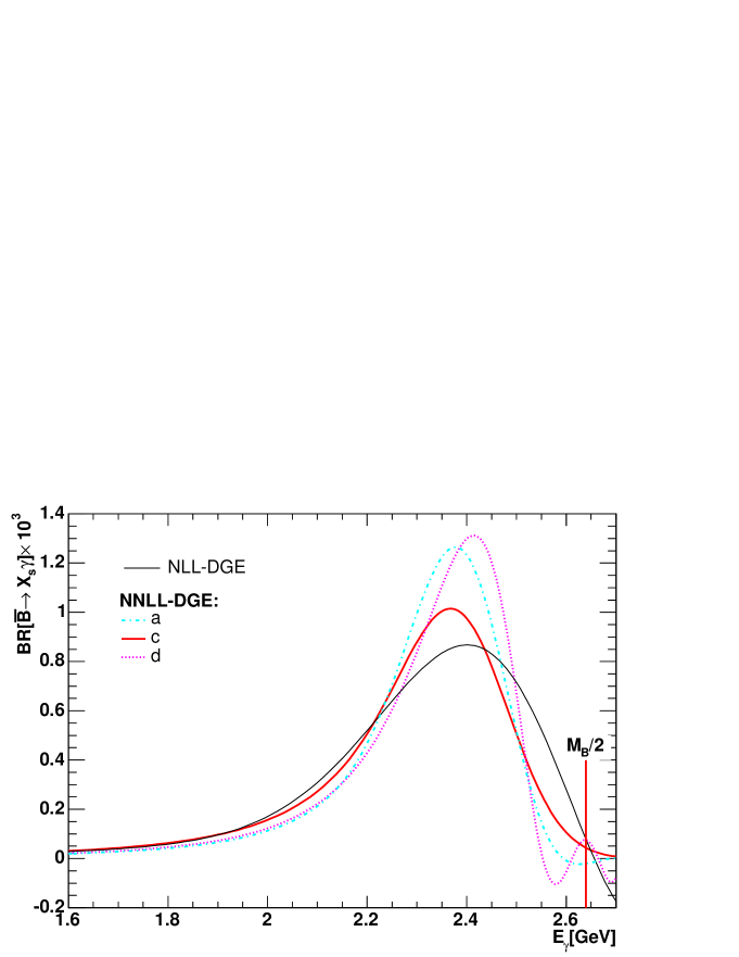
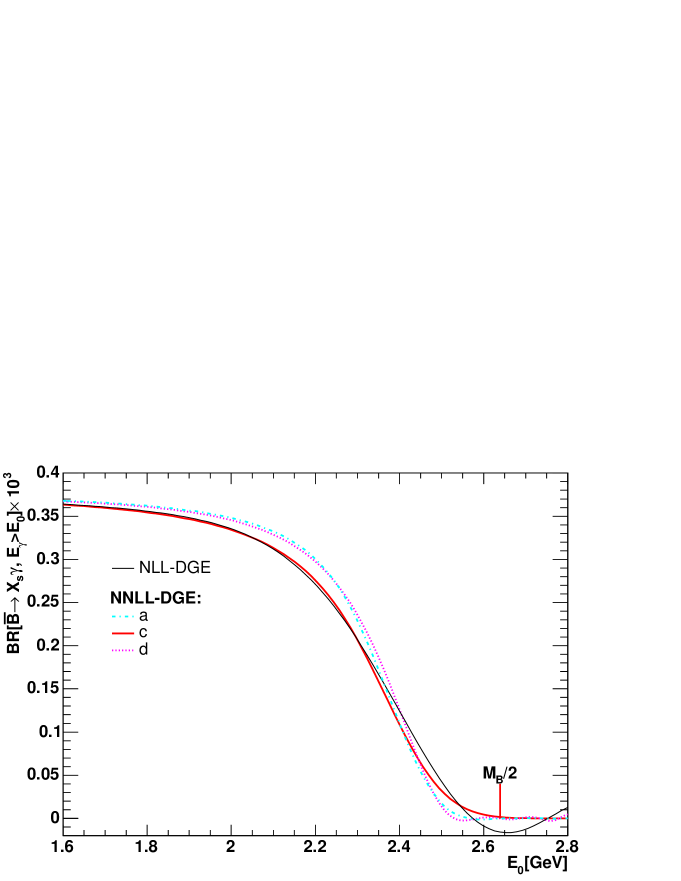
Figure 8: The dependence of the differential (top) and integrated (bottom) $\bar{B}\longrightarrow X_{s}\gamma$ spectrum as predicted by DGE on the model assumed for the Borel function of the soft Sudakov exponent (see Sec. 2.3).

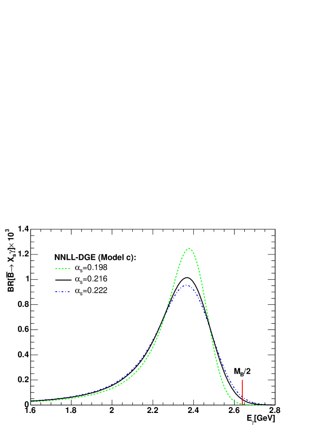
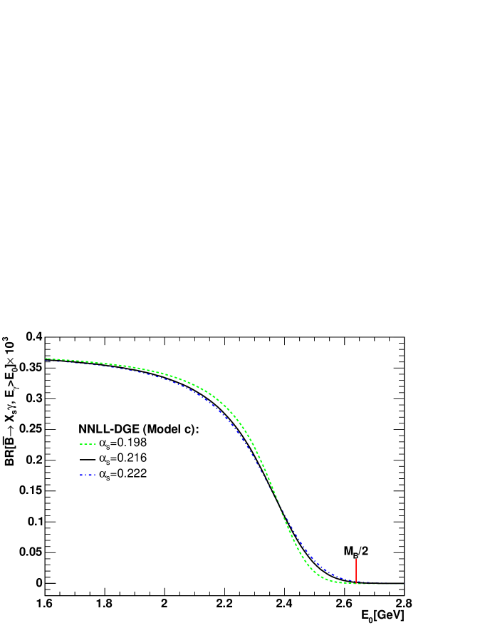
Figure 9: The dependence of the differential (top) and integrated (bottom) $\bar{B}\longrightarrow X_{s}\gamma$ spectrum as predicted by DGE on the value of the strong coupling.

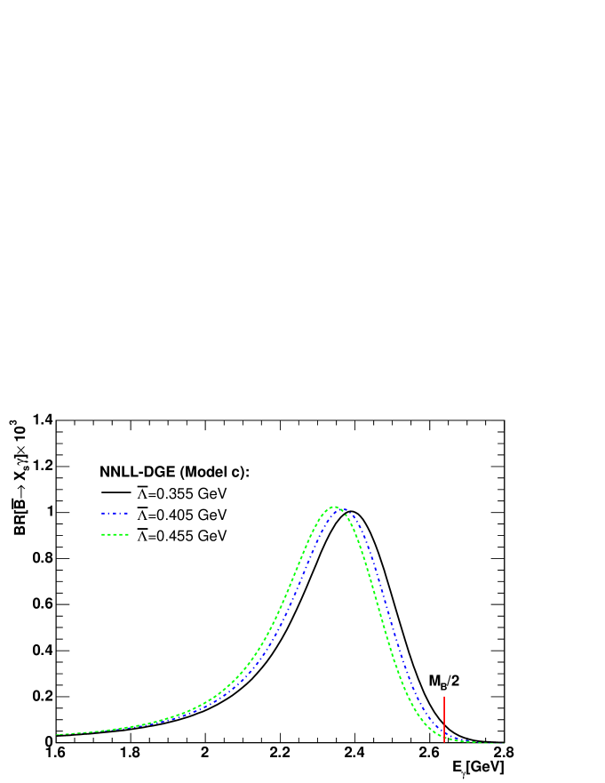
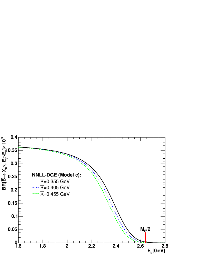
Figure 10: The dependence of the differential (top) and integrated (bottom) $\bar{B}\longrightarrow X_{s}\gamma$ spectrum as predicted by DGE on the assumed value for $\bar{\Lambda}$.

Recall that $M_{N}^{\hbox{\tiny PT},\hbox{\tiny PV}}$ in Eq. (83) is given by Eq. (61), where the DGE Sudakov factor (2.2) is defined in the Principal–Value prescription. As discussed in Sec. 4.1 the use of the corresponding Principal–Value mass $m_{\hbox{\tiny PV}}$ in the definition of $\Delta$ guaranties consistency at the level of the “binding energy”; it effectively accounts for the exponential factor in Eq. (72). On the other hand, additional power corrections ${\cal O}\Big{(}((N-1)\Lambda/M)^{2}\Big{)}$ corresponding to ${\cal F}$ in Eq. (72) are ignored. We are assuming that they are numerically small when using DGE with the Principal–Value prescription. Some evidence that this assumption is sensible is:

• The DGE prediction is perturbatively stable: as shown in Fig. 8 the change from NLL–DGE to NNLL–DGE is moderate. This feature is best seen in moment space, see Fig. 4. Perturbative stability is of course only a necessary condition, not a sufficient one, as not all sources of power corrections can be probed by perturbative means.

• The predicted spectrum smoothly extends beyond the perturbative endpoint and tends to zero for $E_{\gamma}=\left(m+{\cal O}(\Lambda)\right)/2$, close to the physical endpoint $E_{\gamma}=M/2$. In this respect the differences between the various models shown in Fig. 8 are less than 100 MeV. This is quite remarkable given that in the close vicinity of the endpoint all power corrections on the soft scale are a priori important. On the other hand, this should not be taken as an indication that all power corrections are small: they may be large, yet conspire to cancel. Moreover, in the close vicinity of the endpoint the approximation based on keeping power corrections on the soft scale only breaks down: the non-perturbative structure of the jet becomes important; in our formulation resonances are simply ignored.

These are, of course, qualitative arguments. In the long run data will hopefully allow quantifying these power corrections.

The immediate advantage of the DGE calculation of the spectrum is the possibility to provide a reliable estimate of the partial branching fraction and higher moments with experimentally relevant cuts. To assess the remaining theoretical uncertainty in this prediction let us first compare the chosen model $(c)$ for $B_{\cal S}(u)$ (Eq. (2.3)) to other models for the soft Sudakov factor introduced in Sec. 2.3. Recall that the differences between these models are associated with the structure of the Borel function away from the origin, and are therefore equivalent in principle to the power corrections on the soft scale $(m/N)$ that would be parametrized by ${\cal F}$. On the other hand, using the differences between the models as an error estimate is rather conservative, since only model $(c)$ is, by construction, consistent with the large–order behavior of the Sudakov exponent. Fig. 8 shows the differential and integrated spectra according to the various models for $B_{\cal S}(u)$. Differences between models for the differential spectrum near the peak exceed $20\%$. For the integrated spectrum, however, this translates into less than $10\%$ difference for practically any cut (excluding, of course, the immediate vicinity of the endpoint, $E_{0}>2.4$ GeV).

$\alpha_{s}^{\hbox{\tiny${\overline{\rm MS}}$}}(M_{Z})$	$\alpha_{s}^{\hbox{\tiny${\overline{\rm MS}}$}}(m_{\hbox{\tiny PV}})$	$\Lambda_{N_{f}=4}$ GeV	$\bar{\Lambda}_{\hbox{\tiny PV}}=M-m_{\hbox{\tiny PV}}$ GeV
0.113	0.198	0.265	0.392
0.1182	0.216	0.353	0.405
0.120	0.222	0.385	0.455

Table 1: Variation of the parameters entering the calculation of the spectrum with $\alpha_{s}(M_{Z})$.

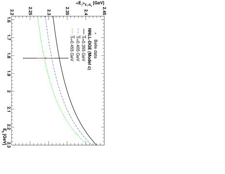
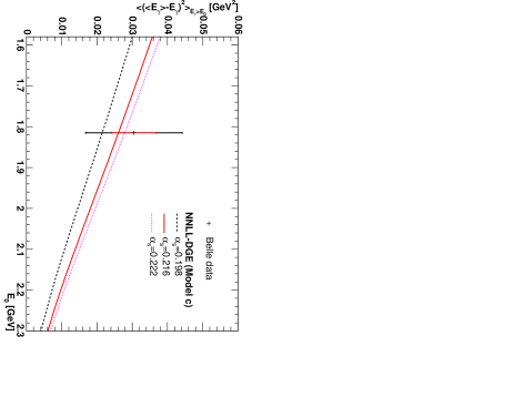
Figure 11: The first two truncated moments of the $\bar{B}\longrightarrow X_{s}\gamma$ spectrum: $\left<E_{\gamma}\right>$ (top) and $\left<(\left<E_{\gamma}\right>-E_{\gamma})^{2}\right>$ (bottom), as a function of the minimum photon energy cut $E_{0}$, as calculated by DGE using model $(c)$ of Eq. (2.3) while varying $\alpha_{s}$ and $m_{\hbox{\tiny${\overline{\rm MS}}$}}$ within their error ranges. In each plot we show a few curves representing the dominant source of uncertainty considering the various models for $B_{\cal S}(u)$ and the values of $\alpha_{s}$ and $m_{\hbox{\tiny${\overline{\rm MS}}$}}$. The DGE result is compared to the available data from Belle [56] with a cut $E_{0}=1.815$ GeV.

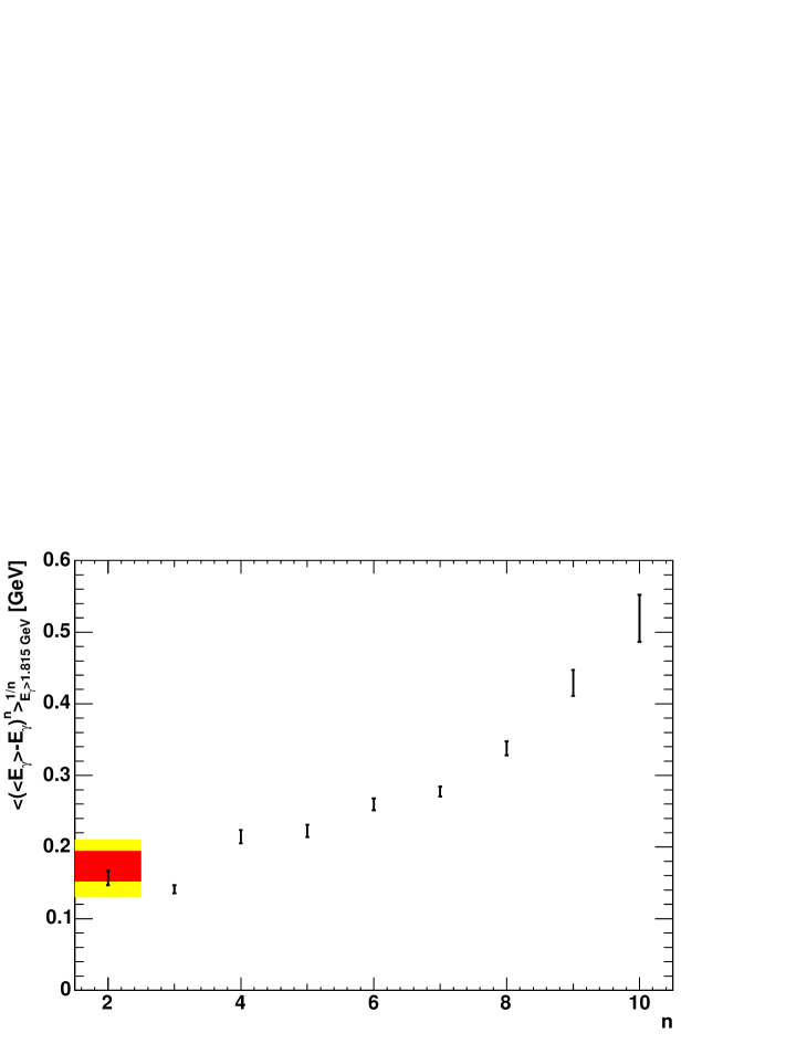
Figure 12: DGE results for the first ten truncated moments of the $\bar{B}\longrightarrow X_{s}\gamma$ spectrum, $\left<(\left<E_{\gamma}\right>-E_{\gamma})^{n}\right>$, with a cut $E_{\gamma}>E_{0}=1.815\,{\rm GeV}$. All moments are presented in energy units (GeV) by taking the corresponding $n$-th root. The $n=2$ result is compared with Belle data, where the internal and external shaded regions represent statistical and statistical plus systematic errors, respectively.

Another theoretical–uncertainty estimate can be obtained by varying the input parameters $\alpha_{s}$ and $m_{\hbox{\tiny${\overline{\rm MS}}$}}$ within their error ranges. The sensitivity of the DGE spectrum to these parameters is higher than in typical short–distance calculations. The precise value of the coupling is important since $\alpha_{s}$ is probed at low scales ${\cal O}(m/N)$. The value of the short–distance mass $m_{\hbox{\tiny${\overline{\rm MS}}$}}$ directly influences the pole mass $m_{\hbox{\tiny PV}}$ (Sec. 4.2), which sets the scale for the spectrum in physical units, see Eq. (4.1). Table 1 details the values of the parameters entering the calculation for the central and the two extreme choices we made for $\alpha_{s}^{\hbox{\tiny${\overline{\rm MS}}$}}(M_{Z})$. Fig. 9 shows the corresponding differential and integrated spectra. Fig. 10 shows the spectrum for the central value of of the coupling, $\alpha_{s}(m)=0.216$, while varying $\bar{\Lambda}$ by $\pm 50$ MeV. This corresponds, to a good approximation, to varying $m_{\hbox{\tiny${\overline{\rm MS}}$}}$ within its error range. Note that while the variation in the coupling influences all the moments (the shape of the distribution gets modified) the variation of $m_{\hbox{\tiny${\overline{\rm MS}}$}}$ mainly affects the average energy: it generates a global shift of the distribution.

A word of caution is due regarding the interpretation of the theoretical uncertainty reflected in the figures. As usual, uncertainty estimates are based on corrections that are known, e.g. degrading the NNLL–DGE to NLL–DGE. In this paper we have not parametrized non-perturbative power corrections, whose influence would increase towards the endpoint. Our analysis only reflects these effects through the different models for $B_{\cal S}(u)$. Such differences might not capture all possible power corrections. In this case, the uncertainty may be underestimated near the endpoint.

Next, let us consider the average of the photon energy with a cut, namely

$$\left<E_{\gamma}\right>_{E_{\gamma}>E_{0}}\equiv\frac{\displaystyle\int_{E_{0}}dE_{\gamma}\,\frac{d\Gamma(E_{\gamma})}{dE_{\gamma}}\,E_{\gamma}}{\displaystyle\int_{E_{0}}dE_{\gamma}\,\frac{d\Gamma(E_{\gamma})}{dE_{\gamma}}}$$ (85)

and, similarly, higher truncated moments:

$$\left<\left(\left<E_{\gamma}\right>_{E_{\gamma}>E_{0}}-E_{\gamma}\right)^{n}\right>_{E_{\gamma}>E_{0}}\equiv\frac{\displaystyle\int_{E_{0}}dE_{\gamma}\,\frac{d\Gamma(E_{\gamma})}{dE_{\gamma}}\,\left(\left<E_{\gamma}\right>_{E_{\gamma}>E_{0}}-E_{\gamma}\right)^{n}}{\displaystyle\int_{E_{0}}dE_{\gamma}\,\frac{d\Gamma(E_{\gamma})}{dE_{\gamma}}}.$$ (86)

Note that these moments differ from the standard Mellin moments discussed so far in two respects: first, they are defined over a limited photon–energy range, and second, these are “central moments” in the sense that they depend of the difference between the photon energy and the average energy in this range.

For sufficiently high $E_{0}$ cuts and low enough $n$ these moments are accessible experimentally. Results for the average energy, Eq. (85), and the variance ($n=2$ in Eq. (86)) were recently published by Belle [56, 57] with $E_{0}=1.815$ GeV. In Fig. 11 we compare this experimental result to our calculation while providing additional theoretical predictions for the dependence on the cut value. We find very good agreement. The experimental error is somewhat larger than the theoretical one. Note that the dominant source of uncertainty in the theoretical prediction for the average energy is the value of $m_{\hbox{\tiny${\overline{\rm MS}}$}}$, affecting the calculation of the pole mass $m_{\hbox{\tiny PV}}$ or $\bar{\Lambda}_{\hbox{\tiny PV}}$. In the future it may even be possible to get an accurate measurement of $m_{\hbox{\tiny${\overline{\rm MS}}$}}$ from experimental data for $\left<E_{\gamma}\right>_{E_{\gamma}>E_{0}}$. On the other hand, the dominant source of uncertainty in the variance is the value of the strong coupling. More interesting comparison can hopefully be done in the future with experimental data having higher cuts, where the systematic experimental errors are expected to be smaller. The possibility to make comparison between theory and data as a function of the cut has an important added value: clearly, at sufficiently high $E_{0}$ values the theoretical prediction, which is lacking any non-perturbative corrections, will fail.

Finally, in Fig. 12 we show the theoretical prediction for the first ten moments. Going to higher moments the finer details of the shape become important. The expectation is, of course, that power corrections will become increasingly important at high $n$. Having excluded power corrections, the dominant source of uncertainty in Fig. 12 is the value of $\alpha_{s}$. Since for higher moments the coupling is probed at lower scales $\sim{\cal O}(m/n)$, this uncertainty gradually increases with $n$. Following Belle [56] we have chosen $E_{\gamma}>E_{0}=1.815\,{\rm GeV}$. Fig. 12 shows the comparison with Belle data for the variance; there is no data to compare with for $n\geq 3$.

6 Conclusions

Inclusive $B$–decay spectra present a special challenge to theory: because of their inclusive nature the details of the hadronic wave function are largely irrelevant, but on the other hand, the soft scales involved prohibit a straightforward perturbative approach.

• The clearest manifestation of the non-perturbative nature of the $\bar{B}\longrightarrow X_{s}\gamma$ spectrum is that any fixed–order perturbative result has support only for $E_{\gamma}<m/2$ while the physical spectrum extends to $E_{\gamma}=M/2$. The gap between the quark pole mass and the meson mass is related to non-perturbative dynamic of the bound state.

• Moreover, the perturbative endpoint region is characterized by parametrically large corrections. The conventional approach to Sudakov resummation, which relies on the dominance of logarithmic corrections in the large–$N$ limit where $\alpha_{s}(m)\ln N$ is fixed, fails because of large running–coupling effects. The breakdown of the perturbative expansion with increasing logarithmic accuracy is demonstrated in Fig. 2 (see also Fig. 2 in [16]).

In this paper we showed that DGE provides a solution to both these problems. Although it is based on resummation of perturbation theory the DGE–resummed spectrum does not have perturbative support. By taking the Principal–Value prescription in moment space this inherent limitation of any fixed–order approximation is removed. The spectrum smoothly extends to the non-perturbative regime and tends to zero for $E_{\gamma}=\left(m+{\cal O}(\Lambda)\right)/2$, qualitatively as expected in the meson decay (see Fig. 6).

Of course, the DGE spectrum does not have correct non-perturbative support properties: it does not strictly vanish for $E_{\gamma}>M/2$. Moreover, is not necessarily positive definite for any $E_{\gamma}<M/2$ (see e.g. Fig. 8). Indeed, the close vicinity of the endpoint is beyond theoretical control as it involves an infinite number of non-perturbative power corrections on the soft scale $m/N$, and eventually also the non-perturbative structure of the jet.

In this work we presented perturbative predictions and refrained from making any parametrization of non-perturbative power corrections. It is conceivable that there exist a region where a few non-perturbative corrections on the soft scale are phenomenologically relevant, while corrections on the jet–mass scale can be ignored. Once experimental data are precise enough, power corrections on the soft scale will be worthwhile parametrizing because of their universal nature: they are related exclusively to the quark distribution in the meson. Therefore, fixing their magnitude can be instrumental to precision measurements of $V_{ub}$ from charmless semileptonic B decays. The DGE spectrum presented here provides a baseline for systematic parametrization of such non-perturbative power corrections. Perturbative stability is imperative in this respect. The remarkable stability of the DGE result (compare Fig. 4 to Fig. 1) is largely thanks to the resummation of running–coupling effects.

It should be emphasized that the difference between DGE and any fixed–logarithmic–accuracy approach is a qualitative one. Recall, that an accurate value of $m_{\hbox{\tiny PV}}$ (or $\bar{\Lambda}_{\hbox{\tiny PV}}$) is essential for the calculation of the photon–energy spectrum in physical units (see Sec. 4). As opposed to the general concept of the pole mass, $m_{\hbox{\tiny PV}}$ has no linear ${\cal O}(\Lambda)$ ambiguity. It can be determined with roughly the same accuracy as short–distance masses ($\sim 50$ MeV). It is only because the Sudakov exponent was defined using the Principal–Value prescription that $m_{\hbox{\tiny PV}}$ becomes the relevant mass. This is a manifestation of the cancellation of renormalon ambiguities between the quark–distribution subprocess in the Sudakov factor and the pole mass [16]. In a fixed–logarithmic–accuracy approach the renormalon in the Sudakov factor is hidden — it is realized through the divergence of the expansion in Eq. (15) — so the choice of mass scheme when computing the spectrum in physical units becomes ad hoc.

Experimentally–favorable observables are moments of the photon–energy spectrum defined over a limited range, $E_{\gamma}>E_{0}$, Eqs. (85) and (86). Having obtained a stable prediction in Mellin space over a wide domain in the complex $N$ plane, we can reliably compute the truncated moments over a range of experimentally–relevant cut values. We showed that our calculation nicely agrees with the recent data from Belle [56]. Furthermore, a great variety of possibilities for comparison between data and theory is now open, e.g. studying the dependence on the cut value and higher truncated moments. In this way more detailed information on the distribution can be systematically extracted. This is, in particular, imperative to quantifying power corrections.

The qualitative success of the DGE calculation presented here, which does not involve any non-perturbative parameters, and the good agreement with the available data from Belle, indicate that additional power corrections in this framework are indeed small. This approach is therefore promising for extracting $V_{ub}$ from charmless semileptonic B decays.

Note added

A few weeks after the submission of this paper, the BaBar collaboration has presented [58] new preliminary data for the partial branching ratio, as well as the average energy and the variance as a function of the cut. Comparison of the predictions in Figs. 10 and 11 above with these measurements can be found in Ref. [59].

Appendix A Singular terms at NNLO

Let us expand the Sudakov exponent in Eq. (15) to ${\cal O}\left(\alpha_{s}^{2}\right)$. We get:

$${\rm Sud}(m,N) = \exp\bigg{\{}\left(\frac{\alpha_{s}^{\hbox{\tiny${\overline{\rm MS}}$}}(m)}{\pi}\right)\bigg{[}-{\displaystyle\frac{1}{2}}\,\ln^{2}N\,{A_{1}}+(-\gamma_{E}\,{A_{1}}-{B_{1}}+{\mathit{D}_{1}})\,\ln N\bigg{]}\,$$

$$+{\left(\frac{\alpha_{s}^{\hbox{\tiny${\overline{\rm MS}}$}}(m)}{\pi}\right)}^{2}\bigg{[}-{\displaystyle\frac{1}{2}}\,{\beta_{0}}\,\ln^{3}N\,{A_{1}}+\left(\left(-{\displaystyle\frac{3}{2}}\,\gamma_{E}\,{A_{1}}+{\mathit{D}_{1}}-{\displaystyle\frac{1}{2}}\,{B_{1}}\right)\,{\beta_{0}}-{\displaystyle\frac{1}{2}}\,{A_{2}}\right)\,\ln^{2}N$$

$$+\left(\left(-\gamma_{E}\,{B_{1}}+2\,\gamma_{E}\,{\mathit{D}_{1}}-{\displaystyle\frac{3}{2}}\,{A_{1}}\,\gamma_{E}^{2}-{\displaystyle\frac{1}{4}}\,{A_{1}}\,\pi^{2}\right)\,{\beta_{0}}-\gamma_{E}\,{A_{2}}-{B_{2}}+{\mathit{D}_{2}}\right)\,\ln N\bigg{]}+\cdots\bigg{\}}$$

To get $\bar{M}_{N}^{\hbox{\tiny PT},\,O_{7}}$ in Eq. (5) one needs the matching coefficient, which is currently known only to ${\cal O}(\alpha_{s})$. It is given by [16]:

$$C_{N}^{O_{7}}(\alpha_{s}(m))=1+\frac{C_{F}\alpha_{s}}{2\pi}\,\bigg{\{}\bigg{[}\left({\displaystyle\frac{7}{2}}-{\displaystyle\frac{1}{N\,(N+1)}}+{\displaystyle\frac{2}{N}}\right)\,\left(\Psi(N)+\gamma_{E}\right)+\Psi_{1}(N)-{\displaystyle\frac{\pi^{2}}{6}}$$

$$\hskip 70.0pt-\left(\Psi(N)+\gamma_{E}\right)^{2}-{\displaystyle\frac{31}{6}}+{\displaystyle\frac{9}{2\,N}}+{\displaystyle\frac{1}{(N+1)^{2}}}-{\displaystyle\frac{1}{N+2}}-{\displaystyle\frac{1}{2\,N+2}}+{\displaystyle\frac{1}{N^{2}}}\bigg{]}$$

$$\hskip 70.0pt-\,\bigg{[}-\ln^{2}N+\left(\frac{7}{2}-2\gamma_{E}\right)\ln N\bigg{]}\bigg{\}}+{\cal O}\left(\alpha_{s}^{2}\right).$$ (88)

Let us note that having fixed the anomalous dimensions as above, the only missing ingredient for Sudakov resummation of decay spectra with NNLL accuracy is the $N$–independent term at ${\cal O}(\alpha_{s}^{2})$.

For easy comparison with future two–loop calculations of the decay process, we summarize below the log–enhanced terms to order $\alpha_{s}^{2}$. Expanding the exponent and taking into account the constant terms at order $\alpha_{s}$ in Eq. (A) we obtain the following log-enhanced terms at ${\cal O}\left(\alpha_{s}^{2}\right)$:

$$\bar{M}_{N}^{\hbox{\tiny PT},\,O_{7}}=1+\bigg{\{}\left({\displaystyle\frac{7}{4}}-{\displaystyle\frac{1}{2N\,(N+1)}}+{\displaystyle\frac{1}{N}}\right)\,\left(\Psi(N)+\gamma_{E}\right)+\frac{1}{2}\Psi_{1}(N)-\frac{1}{2}\left(\Psi(N)+\gamma_{E}\right)^{2}$$

$$\hskip 40.0pt-{\displaystyle\frac{\pi^{2}}{12}}-{\displaystyle\frac{31}{12}}+{\displaystyle\frac{9}{4\,N}}+{\displaystyle\frac{1}{2(N+1)^{2}}}-{\displaystyle\frac{1}{2(N+2)}}-{\displaystyle\frac{1}{4\,(N+1)}}+{\displaystyle\frac{1}{2N^{2}}}\bigg{\}}\,{\frac{\alpha_{s}^{\hbox{\tiny${\overline{\rm MS}}$}}(m)}{\pi}}$$

$$+ \bigg{\{}{\frac{C_{F}^{2}}{8}}\,\ln^{4}N+\bigg{[}{\frac{1}{12}}\,C_{F}\,N_{f}+\left({\frac{\gamma_{E}}{2}}-{\frac{7}{8}}\right)\,C_{F}^{2}-{\frac{11}{24}}\,C_{F}\,C_{A}\bigg{]}\,\ln^{3}N$$

$$+ \bigg{[}\left(-{\frac{13}{144}}+{\frac{\gamma_{E}}{4}}\right)\,C_{F}\,N_{f}+\left(-{\frac{21}{8}}\,\gamma_{E}+{\frac{3}{4}}\,\gamma_{E}^{2}+{\frac{271}{96}}+{\frac{1}{24}}\,\pi^{2}\right)\,C_{F}^{2}$$

$$+ \left({\frac{95}{288}}-{\frac{11\,\gamma_{E}}{8}}+{\frac{\pi^{2}}{24}}\right)\,C_{A}\,C_{F}\bigg{]}\ln^{2}N+\bigg{[}\left(-{\frac{13}{72}}\,\gamma_{E}-{\frac{85}{144}}+{\frac{1}{4}}\,\gamma_{E}^{2}+{\frac{5}{72}}\,\pi^{2}\right)\,C_{F}\,N_{f}$$

$$+ \left(-{\frac{13\,\pi^{2}}{48}}+{\frac{3}{2}}\,\zeta_{3}+{\frac{\gamma_{E}\,\pi^{2}}{12}}-{\frac{425}{96}}+{\frac{\gamma_{E}^{3}}{2}}-{\frac{21\,\gamma_{E}^{2}}{8}}+{\frac{271\,\gamma_{E}}{48}}\right)\,C_{F}^{2}$$

$$+ \left(-{\frac{1}{4}}\,\zeta_{3}-{\frac{67\,\pi^{2}}{144}}+{\frac{\gamma_{E}\,\pi^{2}}{12}}+{\frac{95\,\gamma_{E}}{144}}+{\frac{905}{288}}-{\frac{11\,\gamma_{E}^{2}}{8}}\right)\,C_{A}\,C_{F}\bigg{]}\ln N\bigg{\}}\left({\frac{\alpha_{s}^{\hbox{\tiny${\overline{\rm MS}}$}}\left(m\right)}{\pi}}\right)^{2}+\cdots.$$

Note that the normalization of the rate influences not only constant terms at ${\cal O}(\alpha_{s})$ but also the contributions to the $\ln^{2}N$ and the $\ln^{1}N$ terms at ${\cal O}(\alpha_{s}^{2})$ that are proportional to $C_{F}^{2}$. Here we present the expansion of $\bar{M}_{N}^{\hbox{\tiny PT},\,O_{7}}$, where the $N=1$ moment is exactly 1 by definition. It is straightforward to convert this expansion to other normalization conventions (Eqs. (116) and (3.3) may be useful).

Converting Eq. (A) to $x$ space, the $x\to 1$ singular terms in the $b\longrightarrow X_{s}\gamma$ distribution (from $O_{7}$) up to ${\cal O}(\alpha_{s}^{2})$ are:

$$\left.\frac{1}{\Gamma_{\hbox{\tiny total}}}\frac{d\Gamma}{dx}\right|_{\hbox{\tiny PT},\,O_{7}} = \delta(1-x)+\bigg{\{}-\,\frac{\ln(1-x)}{1-x}-{\frac{7}{4}}\,\frac{1}{1-x}-\frac{1}{2}(1-x)^{2}$$

$$+ \left(\frac{1}{2}\ln(1-x)+\frac{3}{4}\right)(1-x)-\ln(1-x)+\frac{3}{2}\bigg{\}}_{+}\,C_{F}\,{\frac{\alpha_{s}^{\hbox{\tiny${\overline{\rm MS}}$}}(m)}{\pi}}$$

$$+ \bigg{\{}{\frac{C_{F}^{2}}{2}\,\frac{\ln^{3}(1-x)}{1-x}}+\bigg{[}-{\frac{1}{4}}\,C_{F}\,N_{f}+{\frac{11}{8}}\,C_{F}\,C_{A}+{\frac{21}{8}}\,C_{F}^{2}\bigg{]}\,\frac{\ln^{2}(1-x)}{1-x}$$

$$+ \bigg{[}-{\frac{13}{72}}\,C_{F}\,N_{f}+\left(-{\frac{\pi^{2}}{6}}+{\frac{271}{48}}\right)\,C_{F}^{2}+\left({\frac{95}{144}}+{\frac{\pi^{2}}{12}}\right)\,C_{A}\,C_{F}\bigg{]}\,\frac{\ln(1-x)}{1-x}$$

$$+ \bigg{[}\left({\frac{85}{144}}-{\frac{\pi^{2}}{36}}\right)\,C_{F}\,N_{f}+\left(-{\frac{1}{2}}\,\zeta_{3}-{\frac{\pi^{2}}{6}}+{\frac{425}{96}}\right)\,C_{F}^{2}$$

$$+ \left({\frac{1}{4}}\,\zeta_{3}-{\frac{905}{288}}+{\frac{17\,\pi^{2}}{72}}\right)\,C_{A}\,C_{F}\bigg{]}\frac{1}{1-x}\bigg{\}}_{+}\left({\frac{\alpha_{s}^{\hbox{\tiny${\overline{\rm MS}}$}}(m)}{\pi}}\right)^{2}+\cdots.$$

We checked that the terms that are leading in $\beta_{0}$ in Eq. (A) agree with the large–$x$ expansion of Ref. [8].

In Eq. (A) $\{\,\,\}_{+}$ stand for the standard “+” prescription, i.e.

$$\left\{p(z)\right\}_{+}=p(z)-\delta(1-z)\,\int_{0}^{1}p(z)dz,$$ (91)

so, writing

$$\frac{1}{\Gamma_{\hbox{\tiny total}}}\frac{d\Gamma^{\hbox{\tiny PT}}}{dx}(x)=\delta(1-x)+\left\{p(x)\right\}_{+}$$ (92)

the convolution with a smooth test function $f(x)$ (representing non-perturbative corrections) takes the form:

$$\frac{1}{\Gamma_{\hbox{\tiny total}}}\frac{d\Gamma}{dx}(x)=f(x)\left[1-\int_{0}^{x}p(z)dz\right]+\int_{x}^{1}dzp(z)\,\left(\frac{f(x/z)}{z}-f(x)\right),$$ (93)

where both terms are well defined. In moment space, this is equivalent to multiplying the moments of the perturbative distribution $M_{N}^{\hbox{\tiny PT}}$ by the moments on the test function: $F_{N}=\int_{0}^{1}dzz^{N-1}f(z)$.

Appendix B The $u=\frac{1}{2}$ renormalon in the pole mass

In this Appendix we determine the normalization of the $u=\frac{1}{2}$ renormalon in the pole mass. This result is used for the calculation of the pole mass in the Principal–Value prescription in Sec. 4.2 and for the comparison with the soft Sudakov exponent in Sec. 2.3.

Remarkably, the structure of the leading renormalon ambiguity in the pole mass is known exactly. Ref. [34] has shown that, owing to the vanishing of the anomalous dimension of the $\bar{h}_{v}h_{v}$ operator, the linear ultraviolet divergence in the self energy of a static quark has a very simple structure: it is just proportional to the QCD scale $\Lambda$ without any logarithmic corrections. Consequently, the imaginary part associated with the $u=\frac{1}{2}$ infrared renormalon in the pole mass has the same property:

$${\rm Im}\left\{m\right\}={\rm const}\times\Lambda.$$ (94)

This means that, up to an overall normalization constant, the large–order behavior of the relation between the pole mass and any short–distance mass (which is induced by this renormalon) depends only on the coefficients of the $\beta$ function.

Owing to the dominance of the $u=\frac{1}{2}$ renormalon, which sets in already at low orders, the normalization constant can be computed from the perturbative expansion with accuracy of a few percent [35, 36, 37, 38].

The renormalon in the standard Borel representation

Let us first briefly review the standard analysis (more details can be found in [49]). To make use of Eq. (94) one first integrates the renormalization–group equation,

$$\frac{da}{d\ln\mu^{2}}=-a^{2}\Big{[}1+\delta a+\sum_{k=2}^{\infty}\delta_{k}a^{k}\Big{]},$$ (95)

where $a(\mu)=\beta_{0}\alpha_{s}(\mu)/\pi$ and $\delta_{k}=\beta_{k}/\beta_{0}^{k+1}$, writing $\Lambda$ as:

$$\Lambda=\mu\,\exp\left\{-\frac{1}{2a}-\frac{\delta}{2}\ln(a\delta)\right\}\,\times\,\Bigg{[}1+\sum_{k=1}^{\infty}\bar{c}_{k}a^{k}\Bigg{]},$$ (96)

where $\bar{c}_{k}$ are specific combinations of the coefficients of the $\beta$ function; for example:

$$\bar{c}_{1} = \frac{1}{2}\,\Big{[}-{\delta_{2}}+\delta^{2}\Big{]}$$

$$\bar{c}_{2} = \frac{1}{8}\,\Big{[}-2\,{\delta_{3}}+4\,{\delta_{2}}\,\delta-2\,\delta^{3}+{\delta_{2}}^{2}-2\,{\delta_{2}}\,\delta^{2}+\delta^{4}\Big{]}$$

$$\bar{c}_{3} = \frac{1}{48}\,\Big{[}-8\,{\delta_{4}}+6\,{\delta_{2}}\,{\delta_{3}}-{\delta_{2}}^{3}+8\,{\delta_{2}}^{2}+(16\,{\delta_{3}}-12\,{\delta_{2}}^{2})\,\delta$$ (97)

$$\hskip 30.0pt+(3\,{\delta_{2}}^{2}-6\,{\delta_{3}}-24\,{\delta_{2}})\,\delta^{2}+18\,\delta^{3}\,{\delta_{2}}+(8-3\,{\delta_{2}})\,\delta^{4}-6\,\delta^{5}\Big{]}.$$

Then, writing the perturbative relation between the pole mass and the ${\overline{\rm MS}}$ mass in the standard Borel representation (where the Borel variable $z$ is conjugate to $a$),

$${m}/{m_{\hbox{\tiny${\overline{\rm MS}}$}}(m_{\hbox{\tiny${\overline{\rm MS}}$}})} = 1+\frac{C_{F}}{\beta_{0}}\,\int_{0}^{\infty}dzB(z)\,{\rm e}^{-z/a},$$ (98)

the singular part of $B(z)$ near $z=\frac{1}{2}$ can be explicitly written using Eqs. (94) and (96):

$$B(z)={\rm regular}\,\,+\,\frac{q}{(1-2z)^{1+\frac{1}{2}\delta}}\left[1+\sum_{k=1}^{\infty}c_{k}(1-2z)^{k}\right],$$ (99)

where

$$c_{k}\equiv\frac{\Gamma(1+\frac{\delta}{2}-k)}{2^{k}\,\Gamma(1+\frac{\delta}{2})}\,\bar{c}_{k}.$$ (100)

To see this one inserts Eq. (99) into Eq. (98) and takes the imaginary part of the integral, getting:

$${\rm Im}\Big{\{}{m}/{m_{\hbox{\tiny${\overline{\rm MS}}$}}(m_{\hbox{\tiny${\overline{\rm MS}}$}})}\Big{\}}=\frac{C_{F}}{\beta_{0}}\,\frac{q}{\Gamma(1+\frac{\delta}{2})}\frac{\pi}{2}\left(2a\right)^{-\delta/2}{\rm e}^{-1/(2a)}\,\times\left[1+\sum_{k=1}^{\infty}\bar{c}_{k}a^{k}\right].$$ (101)

In this calculation one uses the following formula:

$$I_{z_{0}}(a)\equiv{\rm Im}\int_{0}^{\infty}dz\frac{{\rm e}^{-z/a}}{(1-z/z_{0})^{1+\kappa}}=\pi\left(\frac{z_{0}}{a}\right)^{\kappa}\,\frac{z_{0}\,{\rm e}^{-z_{0}/a}}{\Gamma(1+\kappa)},$$ (102)

which is derived assuming that $z_{0}$ has an infinitesimally small positive imaginary part. Eq. (101) clearly has exactly the same dependence on the coupling as Eq. (96), so the requirement of Eq. (94) is satisfied.

Figure 13: The normalization constant of the $u=\frac{1}{2}$ renormalon of the pole mass ($C_{F}q/\pi$) as a function of $1/\beta_{0}$. The exact result of the large–$\beta_{0}$ limit is denoted by a cross. Calculations relying on the perturbative expansion of $m/m_{\hbox{\tiny${\overline{\rm MS}}$}}(m_{\hbox{\tiny${\overline{\rm MS}}$}})$: standard Borel transform of the mass ratio in ${\overline{\rm MS}}$ (dotdashes); scheme–invariant Borel transform of the mass ratio (full line); the latter optimized using Eq. (113) (plus signs). Squares represent the calculation relying on the scheme–invariant Borel transform of the soft Sudakov exponent and on the cancellation of the ambiguity (i.e. on Eq. (34)). This calculation uses an optimization procedure similar to the one of Eq. (113).

The pole mass (and its imaginary part) is renormalization–scheme invariant. Several authors have computed the normalization constant $q$ using the perturbative expansion of ${m}/{m_{\hbox{\tiny${\overline{\rm MS}}$}}(m_{\hbox{\tiny${\overline{\rm MS}}$}})}$ in the ${\rm{\overline{MS}}}$ scheme [35, 36, 37, 38]. This perturbative relation is available to ${\cal O}(\alpha_{s}^{3})$ — see Eq. (10) in [41] (the ${\overline{\rm MS}}$ mass anomalous dimension has been computed before [42]). Knowing that $z=\frac{1}{2}$ is the nearest singularity to the origin and using Eq. (99) one can extract the residue by first multiplying [39, 40] the available $n$-th order approximation of $B(z)$ by $(1-2z)^{1+\frac{1}{2}\delta}$, then expanding in powers of $z$ and truncating at order $n$ and finally substituting $z=\frac{1}{2}$. We performed this calculation and we agree with previous results. The residue is shown in Fig. 13 as a function of $\beta_{0}$. For example, we obtained: $C_{F}q(N_{f}\longrightarrow\infty)/\pi\simeq 0.935$ and $C_{F}q(N_{f}=4)/\pi\simeq 0.551$. We estimate the error on this determination as $\sim 3\%$. This estimate is based on comparison with a similar calculation using the scheme invariant Borel transform (see below) and on the one point where the exact value of the normalization constant has been computed [27], the large–$\beta_{0}$ limit. There $B(z)$ is

$$\left.B(z)\right|_{\rm large\beta_{0}}={\rm regular}+\frac{3}{2}{\rm e}^{\frac{5}{3}z}\,\frac{(1-z)\Gamma(z)\Gamma(1-2z)}{\Gamma(3-z)}.$$ (103)

where the regular terms are related with the renormalization of the ${\overline{\rm MS}}$ mass. Thus the exact value is $C_{F}q(N_{f}\longrightarrow\infty)/\pi=C_{F}{\rm e}^{\frac{5}{6}}/\pi\simeq 0.9766$.

To clarify the relation between the normalization constant in the scheme–invariant Borel transform and in the standard one, let us first consider the latter in different renormalization schemes. First, let us stress that having fixed the definition of $\Lambda$ in Eq. (96), the scheme (and thus the value of the coupling at the scale $\mu$) depend on all the $\beta$–function coefficients $\beta_{k}$ with $k\geq 2$. We note that while the sum in Eq. (99) converges, the significance of subleading terms there strongly depends on the scheme. In particular, we find that in a scheme $({\rm RS})$ where the $\beta$–function coefficients are characterized by geometrical progression, ${da_{\hbox{\tiny RS}}}/{d\ln\mu^{2}}=-{a_{\hbox{\tiny RS}}^{2}}/\left({1-\delta a_{\hbox{\tiny RS}}}\right)$, all the coefficients $c_{k}$ vanish. On the other hand in the ’t Hooft scheme of Eq. (2.2), one obtains $c_{k}^{\hbox{\tiny't Hooft}}=(\delta/2)^{k}/k!$, so the singular part of the Borel function sums up into:

$$B(z)={\rm regular}\,\,+\,\frac{q\,{\rm e}^{\delta\left(\frac{1}{2}-z\right)}}{(1-2z)^{1+\frac{1}{2}\delta}}.$$ (104)

and

$$\bar{c}_{k}^{\hbox{\tiny't Hooft}}=\frac{\delta^{k}\,\Gamma(1+\frac{\delta}{2})}{\Gamma(k+1)\Gamma(1+\frac{\delta}{2}-k)},$$

so the imaginary part in Eq. (101) sums up into:

$${\rm Im}\Big{\{}{m}/{m_{\hbox{\tiny${\overline{\rm MS}}$}}(m_{\hbox{\tiny${\overline{\rm MS}}$}})}\Big{\}}=\frac{C_{F}}{\beta_{0}}\,\frac{q}{\Gamma(1+\frac{\delta}{2})}\frac{\pi}{2}\,\left(\frac{1+\delta A}{2A}\right)^{\delta/2}\,{\rm e}^{-1/(2A)},$$ (105)

where the ’t Hooft coupling $A$ is evaluated at $m_{\hbox{\tiny${\overline{\rm MS}}$}}(m_{\hbox{\tiny${\overline{\rm MS}}$}})$. The same result can be obtained by substituting Eq. (104) into Eq. (98) (where $a$ is replaced by the ’t Hooft coupling $A$) and evaluating the integral using the relation:

$$\int_{0}^{\infty}duT(u)\left(\Lambda^{2}/\mu^{2}\right)^{u}\frac{1}{u-u_{0}}=-\frac{1}{u_{0}}\int_{0}^{\infty}dz{\rm e}^{-z/A}\frac{{\rm e}^{-z\delta}}{\left(1-\frac{z}{u_{0}}\right)^{1+u_{0}\delta}},$$ (106)

where $T(u)$ and the relation between $A$ and $\ln\mu^{2}/\Lambda^{2}$ are given in Eq. (2.2). The imaginary part of the l.h.s. is simply $-\pi$ times the residue at $u=\frac{1}{2}$. This exercise also shows that the scheme invariant formulation is most natural for the problem at hand: the singular part of the corresponding Borel function is just a simple pole.

The renormalon in the scheme–invariant Borel representation

Let us turn now to consider the pole–mass renormalon in the scheme–invariant formulation of the Borel transform. The mass ratio is expressed as

$${m}/{m_{\hbox{\tiny${\overline{\rm MS}}$}}(m_{\hbox{\tiny${\overline{\rm MS}}$}})}=1+\frac{C_{F}}{\beta_{0}}\int_{0}^{\infty}du\,T(u)B(u)\,\left(\frac{\Lambda^{2}}{m_{\hbox{\tiny${\overline{\rm MS}}$}}^{2}(m_{\hbox{\tiny${\overline{\rm MS}}$}})}\right)^{u},$$ (107)

where as in Eq. (2.2), $T(u)$ corresponds to the ’t Hooft scheme.

Taking the imaginary part of Eq. (107) we obtain:

$${\rm Im}\Big{\{}{m}/{m_{\hbox{\tiny${\overline{\rm MS}}$}}(m_{\hbox{\tiny${\overline{\rm MS}}$}})}\Big{\}}=-\frac{C_{F}}{\beta_{0}}R\times J_{\frac{1}{2}}\Big{(}m_{\hbox{\tiny${\overline{\rm MS}}$}}(m_{\hbox{\tiny${\overline{\rm MS}}$}})\Big{)}$$ (108)

where the residue is

$$R\equiv\lim_{u\to\frac{1}{2}}\left(u-\frac{1}{2}\right)B(u)$$ (109)

and

$$J_{u_{0}}(\mu) \equiv {\rm Im}\int_{0}^{\infty}du\,T(u)\,\left(\frac{\Lambda^{2}}{\mu^{2}}\right)^{u}\frac{1}{u-u_{0}-i\epsilon}=\pi T(u_{0})\left(\frac{\Lambda^{2}}{\mu^{2}}\right)^{u_{0}}\!\!\!=\pi\left(\frac{u_{0}}{\tilde{A}}\right)^{u_{0}\delta}\frac{{\rm e}^{-u_{0}/{\tilde{A}}}}{\Gamma(1+u_{0}\delta)}$$

where $\epsilon>0$ is infinitesimally small; the two expressions were obtained based on the residue theorem and Eq. (106), respectively. In the second expression $\tilde{A}(\mu)$ is defined by

$$\frac{1}{\tilde{A}}=\frac{1}{A}+\delta,$$ (111)

or, equivalently, $\ln\left(\mu^{2}/\Lambda^{2}\right)={1}/{\tilde{A}}\,-\,\delta\,+\,\delta\ln(\delta\tilde{A})$. Comparing Eq. (108) with Eq. (105) we find that

$$q=-2R\,{\rm e}^{-\delta/2}.$$ (112)

The approximate calculation of the residue $R$ based on the perturbative expansion proceeds similarly to the standard Borel transform: one multiplies by $(\frac{1}{2}-u)$ expands and uses the truncated series to compute the value at $u=\frac{1}{2}$. The result is shown in as a function of $1/\beta_{0}$ in Fig. 13, where the comparison with the standard Borel transform is available. One can repeat the calculation by first multiplying the truncated series by an arbitrary function $f(u)$ (which has a Taylor expansion at $u=0$ that converges at least for $|u|\leq\frac{1}{2}$), then taking the limit, and finally dividing by the exact value $f(\frac{1}{2})$,

$$R_{\hbox{\tiny opt}}\equiv\frac{1}{f(\frac{1}{2})}\,\lim_{u\to\frac{1}{2}}\left(u-\frac{1}{2}\right)B(u)f(u).$$ (113)

We have chosen the set of functions: $f(u)=\exp(\tau u)$ where $\tau$ is arbitrary. A reliable approximation should be independent of variations of the function $f(u)$. Therefore, the procedure can be improved by finding a saddle point with respect to $\tau$. The result of this optimized calculation of $R$ are shown in Fig. 13 as well. It turns out that the result is quite stable so the difference between the optimized calculation and the simple one is small, for example, for $C_{F}q(N_{f}=4)/\pi$ we get $0.5355$ and $0.5363$ in the two, respectively.

In conclusion, the normalization of the $u=\frac{1}{2}$ renormalon in the pole mass can be determined from the perturbative relation with the ${\overline{\rm MS}}$ mass within a few percent. The difference between the determination using the scheme–invariant Borel representation and the one using the standard Borel representation is somewhat larger than the variation of the results within each of the two approaches.

Appendix C NLO results for $b\longrightarrow s\gamma g$ and the matching procedure

We begin with the well-known expressions for the $b\longrightarrow s\gamma g$ contributions [45]:

$$\phi_{22}(\Delta) = \frac{4z}{9}\left[\Delta\int_{0}^{(1-\Delta)/z}dt\;(1-zt)\left|\frac{G(t)}{t}+\frac{1}{2}\right|^{2}\;+\;\int_{(1-\Delta)/z}^{1/z}dt\;(1-zt)^{2}\left|\frac{G(t)}{t}+\frac{1}{2}\right|^{2}\right],$$

$$\phi_{27}(\Delta) = -\frac{2z^{2}}{3}\left[\Delta\int_{0}^{(1-\Delta)/z}dt\;{\rm Re}\left(G(t)+\frac{t}{2}\right)\;+\;\int_{(1-\Delta)/z}^{1/z}dt\;(1-zt){\rm Re}\left(G(t)+\frac{t}{2}\right)\right],$$

$$\phi_{77}(\Delta) = \frac{5}{2}\Delta+\frac{1}{4}\Delta^{2}-\frac{1}{6}\Delta^{3}+\frac{1}{4}\Delta(\Delta-4)\ln\Delta,$$ (114)

$$\phi_{78}(\Delta) = \frac{2}{3}\left[{\rm Li}_{2}(1-\Delta)-\frac{\pi^{2}}{6}-\Delta\ln\Delta+\frac{9}{4}\Delta-\frac{1}{4}\Delta^{2}+\frac{1}{12}\Delta^{3}\right],$$

$$\phi_{88}(\Delta) = \frac{1}{36}\left\{-2\ln\frac{m_{b}}{m_{s}}\left[\Delta^{2}+2\Delta+4\ln(1-\Delta)\right]\right.$$

$$\hskip 28.45274pt\left.+4{\rm Li}_{2}(1-\Delta)-\frac{2\pi^{2}}{3}-\Delta(2+\Delta)\ln\Delta+8\ln(1-\Delta)-\frac{2}{3}\Delta^{3}+3\Delta^{2}+7\Delta\right\},$$

$$\phi_{11} = \frac{1}{36}\phi_{22},~{}~{}~{}~{}~{}~{}\phi_{12}=-\frac{1}{3}\phi_{22},~{}~{}~{}~{}~{}~{}\phi_{17}=-\frac{1}{6}\phi_{27},~{}~{}~{}~{}~{}~{}\phi_{18}=\frac{1}{18}\phi_{27},~{}~{}~{}~{}~{}~{}\phi_{28}=-\frac{1}{3}\phi_{27},$$

where

$$G(t)=\left\{\begin{array}[]{cc}-2\arctan^{2}\sqrt{\frac{t}{4-t}},&\mbox{ for $t<4$}\vspace{0.3cm}\\ -\frac{\pi^{2}}{2}+2\ln^{2}\frac{\sqrt{t}+\sqrt{t-4}}{2}-2i\pi\ln\frac{\sqrt{t}+\sqrt{t-4}}{2},&\mbox{ for $t\geq 4$}.\end{array}\right.$$

and where, following [44], we use $z\equiv m_{c}^{\hbox{\tiny${\overline{\rm MS}}$}}(\mu)/m_{b}\simeq 0.22\pm 0.04$.

As explained in Sec. 3 our matching procedure involves splitting some of these functions, $\phi_{ij}(\Delta)=\eta_{ij}(\Delta)+\xi_{ij}(\Delta)$, such that $\eta_{ij}(\Delta)$ dominates the small–$\Delta$ limit. We require: $\xi_{ij}(\Delta)={\cal O}(\Delta^{2})$.

For $\phi_{77}$, which is conveniently transformed to moment space we simply define $\eta_{77}(\Delta)=\phi_{77}(\Delta)$ and $\xi_{77}(\Delta)=0$. It then follows from Eq. (62) that

$$\mu_{77}(N) = \frac{1}{2}\left[\left(\Psi(N)+\gamma_{E}\right)\,\left(\frac{1}{1+N}+\frac{1}{N}\right)-\frac{1}{2}\frac{1}{N+1}-\frac{1}{N+2}+\frac{9}{2N}+\frac{1}{(N+1)^{2}}+\frac{1}{N^{2}}\right].$$

Note that in Eq. (61) the full $O_{7}$ contribution is reproduced by $f(N)+\mu_{77}(N)$ plus the single and double logs from the expansion of ${\rm Sud}(m,N)$ (these are the ${\cal O}(\alpha_{s})$ terms in Eq. (A)). Note also that $f(N)+\mu_{77}(N)$ differs from $C_{N}^{O_{7}}$ of Eq. (A) by the constant term $\frac{31}{12}$, the reason being that the latter corresponds to the moments $\bar{M}^{\hbox{\tiny PT},\,O_{7}}_{N}$ (of the normalized rate) while the former corresponds to the moments $M^{\hbox{\tiny PT},\,O_{7}}_{N}$; indeed $\mu_{77}(N=1)=\phi_{77}(\Delta=1)=\frac{31}{12}$ so

$$M_{N}^{O_{7}}=\bar{M}_{N}^{O_{7}}\times\left(1+\frac{C_{F}\alpha_{s}}{\pi}\,\frac{31}{12}+{\cal O}(\alpha_{s}^{2})\right).$$ (116)

Similarly, for $\phi_{78}$, we define: $\eta_{78}(\Delta)=\phi_{78}(\Delta)$ and $\xi_{78}(\Delta)=0$, so

$$\mu_{78}(N) = \frac{2}{3}\left[-\frac{1}{(N-1)N}(\Psi(N)+\gamma_{E})+\frac{1}{N^{2}}+\frac{1}{4}\frac{1}{N+2}+\frac{1}{N}\right].$$ (117)

As explained in the text, the treatment of the other contributions involves splitting the real–emission terms into two. For all the contributions associated with the operators $O_{1}$ and $O_{2}$ and their interference with $O_{7}$ and $O_{8}$ (this includes $\phi_{22}$, $\phi_{27}$, $\phi_{11}$, $\phi_{12}$ $\phi_{17}$, $\phi_{18}$ and $\phi_{28}$) we define

$$\dot{\phi}_{ij}\equiv\left.\frac{d\phi_{ij}(\Delta)}{d\Delta}\right|_{\Delta=0}$$

and write:

$$\eta_{ij}(\Delta) = \dot{\phi}_{ij}\,\Delta,$$

$$\xi_{ij}(\Delta) = \phi_{ij}(\Delta)-\dot{\phi}_{ij}\,\Delta.$$

Since the derivative of $\eta_{ij}(\Delta)$ is a constant, the moments in Eq. (62) are pure $1/N$ terms:

$$\mu_{ij}(N)=\frac{\dot{\phi}_{ij}}{N}.$$ (118)

Finally, the contribution of $\phi_{88}$ it taken into account by extracting the leading term at $\Delta\longrightarrow 0$ (which makes the corresponding contribution to the differential rate singular) and incorporating it in moment space:

$$\eta_{88}(\Delta) = \frac{1}{9}\left[\ln\frac{m_{b}}{m_{s}}-\frac{5}{4}+\frac{1}{2}\ln\Delta\right]\,\Delta,$$

$$\xi_{88}(\Delta) = \phi_{88}(\Delta)-\eta_{88}(\Delta),$$

so

$$\mu_{88}(N)=\frac{1}{3N}\left[\frac{1}{3}\ln\frac{m_{b}}{m_{s}}-\frac{1}{4}-\frac{1}{6}(\Psi(N)+\gamma_{E})-\frac{1}{6}\frac{1}{N}\right].$$ (119)

As follows from their definition all $\mu_{ij}(N)$ vanish at large $N$.

Finally, let us summarize the result for the first moment which enters the expression for the total rate (Eq. (69) with $\Delta\longrightarrow 1$):

$$M_{N=1}^{\hbox{\tiny PT}}=1+\frac{C_{F}\alpha_{s}(m_{b})}{\pi}\!\!\sum_{\scriptsize\begin{array}[]{c}{i,j=1..8}\\ {i\leq j}\end{array}}c_{ij}\,\mu_{ij}(N=1)$$ (120)

with

$$\mu_{77}(N=1) = \frac{31}{12}$$

$$\mu_{78}(N=1) = \frac{25}{18}-\frac{\pi^{2}}{9}$$

$$\mu_{88}(N=1) = \frac{1}{9}\left(\ln\frac{m_{b}}{m_{s}}-\frac{5}{4}\right)$$

$$\mu_{22}(N=1) = \frac{4z}{9}\int_{0}^{1/z}dt\,(1-zt)\left|\frac{G(t)}{t}-\frac{1}{2}\right|^{2}$$

$$\mu_{27}(N=1) = -\frac{2z^{2}}{3}\int_{0}^{1/z}dt\,{\rm Re}\left(G(t)+\frac{t}{2}\right);$$ (121)

The remaining $\mu_{ij}(N=1)$ values can be obtained from the above using the relations in the last line in Eq. (C).

References

- [1] M. Neubert, Phys. Rev. D49 (1994) 4623; [hep-ph/9312311]. Phys. Rev. D49 (1994) 3392 [hep-ph/9311325].
- [2] I. I. Y. Bigi, M. A. Shifman, N. G. Uraltsev and A. I. Vainshtein, Int. J. Mod. Phys. A9 (1994) 2467 [hep-ph/9312359].
- [3] A. F. Falk, E. Jenkins, A. V. Manohar and M. B. Wise, Phys. Rev. D49 (1994) 4553 [hep-ph/9312306].
- [4] G. P. Korchemsky and G. Sterman, Phys. Lett. B340, 96 (1994) [hep-ph/9407344].
- [5] C. W. Bauer, Phys. Rev. D57 (1998) 5611 [Erratum-ibid. D 60 (1999) 099907] [hep-ph/9710513].
- [6] A. L. Kagan and M. Neubert, Eur. Phys. J. C7, 5 (1999) [hep-ph/9805303].
- [7] A. K. Leibovich and I. Z. Rothstein, Phys. Rev. D61 (2000) 074006 [hep-ph/9907391].
- [8] Z. Ligeti, M. E. Luke, A. V. Manohar and M. B. Wise, Phys. Rev. D60 (1999) 034019 [hep-ph/9903305].
- [9] C. W. Bauer, S. Fleming and M. E. Luke, Phys. Rev. D63 (2001) 014006 [hep-ph/0005275].
- [10] C. W. Bauer and A. V. Manohar, Phys. Rev. D70 (2004) 034024 [hep-ph/0312109].
- [11] S. W. Bosch, B. O. Lange, M. Neubert and G. Paz, Nucl. Phys. B699 (2004) 335 [hep-ph/0402094].
- [12] U. Aglietti and G. Ricciardi, Phys. Rev. D66 (2002) 074003 [hep-ph/0204125].
- [13] U. Aglietti and G. Ricciardi, Phys. Rev. D70, (2004) 114008 [hep-ph/0407225].
- [14] M. Neubert, Eur. Phys. J. C40 (2005) 165 [hep-ph/0408179v2].
- [15] D. Benson, I. I. Bigi and N. Uraltsev, Nucl. Phys. B710, 371 (2005) [hep-ph/0410080].
- [16] E. Gardi, JHEP 0404, 049 (2004) [hep-ph/0403249].
- [17] E. Gardi, “Inclusive B decay spectra and IR renormalons”, Proceedings of ‘Workshop on Continuous Advances in QCD 2004’, Minneapolis, Minnesota, 13-16 May 2004. published by World Scientific, T. Gherghetta (Ed.) [hep-ph/0407322].
- [18] E. Gardi and G. Grunberg, JHEP 9911 (1999) 016 [hep-ph/9908458].
- [19] E. Gardi and J. Rathsman, Nucl. Phys. B609 (2001) 123 [hep-ph/0103217];
- [20] E. Gardi and J. Rathsman, Nucl. Phys. B638 (2002) 243 [hep-ph/0201019].
- [21] E. Gardi, Nucl. Phys. B622 (2002) 365 [hep-ph/0108222].
- [22] M. Cacciari and E. Gardi, Nucl. Phys. B664 (2003) 299 [hep-ph/0301047].
- [23] G. Sterman, Nucl. Phys. B281 (1987) 310.
- [24] S. Catani and L. Trentadue, Nucl. Phys. B327 (1989) 323; Nucl. Phys. B353 (1991) 183.
- [25] J. C. Collins, D. E. Soper and G. Sterman, Adv. Ser. Direct. High Energy Phys. 5 (1988) 1 [hep-ph/0409313].
- [26] S. Catani, L. Trentadue, G. Turnock and B. R. Webber, Nucl. Phys. B407 (1993) 3.
- [27] M. Beneke and V. M. Braun, Nucl. Phys. B426, 301 (1994) [hep-ph/9402364].
- [28] I. I. Y. Bigi, M. A. Shifman, N. G. Uraltsev and A. I. Vainshtein, Phys. Rev. D50, 2234 (1994) [hep-ph/9402360].
- [29] S. Moch, J. A. M. Vermaseren and A. Vogt, Nucl. Phys. B688 (2004) 101 [hep-ph/0403192].
- [30] E. Gardi, JHEP 0502 (2005) 053 [hep-ph/0501257].
- [31] A. Vogt, Phys. Lett. B497 (2001) 228 [hep-ph/0010146].
- [32] E. Gardi and R. G. Roberts, Nucl. Phys. B653, 227 (2003) [hep-ph/0210429].
- [33] G. Grunberg, Phys. Lett. B304, 183 (1993).
- [34] M. Beneke, Phys. Lett. B344 (1995) 341 [hep-ph/9408380].
- [35] A. Pineda, JHEP 0106 (2001) 022 [hep-ph/0105008].
- [36] T. Lee, JHEP 0310, 044 (2003) [hep-ph/0304185].
- [37] G. Cvetic, J. Phys. G 30 (2004) 863 [hep-ph/0309262].
- [38] Nikolaus Warkentin, “Perturbative and non-perturbative aspects of deep-inelastic scattering in the semi-inclusive region,” Diploma thesis, Universität Regensburg, June 2004.
- [39] T. Lee, Phys. Lett. B462 (1999) 1 [hep-ph/9908225].
- [40] G. Cvetic and T. Lee, Phys. Rev. D64 (2001) 014030 [hep-ph/0101297].
- [41] K. Melnikov and T. v. Ritbergen, Phys. Lett. B482 (2000) 99 [hep-ph/9912391].
- [42] J. A. M. Vermaseren, S. A. Larin and T. van Ritbergen, Phys. Lett. B405 (1997) 327 [hep-ph/9703284].
- [43] M. Neubert, Phys. Lett. B393 (1997) 110 [hep-ph/9610471].
- [44] P. Gambino and M. Misiak, Nucl. Phys. B611 (2001) 338 [hep-ph/0104034].
- [45] K. G. Chetyrkin, M. Misiak and M. Munz, Phys. Lett. B400 (1997) 206 [Erratum-ibid. B425 (1998) 414] [hep-ph/9612313].
- [46] A. J. Buras and M. Misiak, Acta Phys. Polon. B33 (2002) 2597 [hep-ph/0207131].
- [47] A. J. Buras, A. Czarnecki, M. Misiak and J. Urban, Nucl. Phys. B631 (2002) 219 [hep-ph/0203135].
- [48] J. H. Kuhn and M. Steinhauser, Nucl. Phys. B619 (2001) 588 [Erratum-ibid. B640 (2002) 415] [hep-ph/0109084].
- [49] M. Beneke, Phys. Rept. 317 (1999) 1 [hep-ph/9807443].
- [50] J. A. Gracey, Phys. Lett. B322 (1994) 141 [hep-ph/9401214]; Nucl. Phys. B480 (1996) 73 [hep-ph/9609301].
- [51] M. Beneke and V. M. Braun, Nucl. Phys. B454 (1995) 253 [hep-ph/9506452].
- [52] G. P. Korchemsky and A. V. Radyushkin, Phys. Lett. B279 (1992) 359 [hep-ph/9203222].
- [53] G. P. Korchemsky and G. Marchesini, Nucl. Phys. B406 (1993) 225 [hep-ph/9210281]; Phys. Lett. B313 (1993) 433.
- [54] G. P. Korchemsky and A. V. Radyushkin, Nucl. Phys. B283 (1987) 342.
- [55] G. P. Korchemsky, Mod. Phys. Lett. A4 (1989) 1257.
- [56] P. Koppenburg et al. [Belle Collaboration], Phys. Rev. Lett. 93 (2004) 061803 [hep-ex/0403004].
- [57] A. Limosani and T. Nozaki [Heavy Flavor Averaging Group Collaboration], “Extraction of the b-quark shape function parameters using the Belle B photon–energy spectrum,” [hep-ex/0407052].
- [58] J.J. Walsh [BaBar Coll.] “Semileptonic and EW Penguin Decay Results from BaBar”, Talk at the 40th Rencontres de Moriond ‘QCD and Hadronic Interactions’, La Thuile, Italy, March 12 – 19, 2005. http://moriond.in2p3.fr/QCD/2005/Index.html
- [59] E. Gardi and J. R. Andersen, “A new approach to inclusive decay spectra”, Proceedings of the 40th Rencontres de Moriond ‘QCD and Hadronic Interactions’, La Thuile, Italy, March 12 – 19, 2005 [hep-ph/0504140].