Geotomography with solar and supernova neutrinos

Abstract:

We show how by studying the Earth matter effect on oscillations of solar and supernova neutrinos inside the Earth one can in principle reconstruct the electron number density profile of the Earth. A direct inversion of the oscillation problem is possible due to the existence of a very simple analytic formula for the Earth matter effect on oscillations of solar and supernova neutrinos. From the point of view of the Earth tomography, these oscillations have a number of advantages over the oscillations of the accelerator or atmospheric neutrinos, which stem from the fact that solar and supernova neutrinos are coming to the Earth as mass eigenstates rather than flavour eigenstates. In particular, this allows reconstruction of density profiles even over relatively short neutrino path lengths in the Earth, and also of asymmetric profiles. We study the requirements that future experiments must meet to achieve a given accuracy of the tomography of the Earth.

1 Introduction

The idea to use neutrinos in order to probe the interior of the Earth was originally put forward more than 30 years ago Volkova , and since then has undergone a number of improvements and modifications DeRujula:1983ya , Wilson:1983an , Askarian:ca , Borisov:sm , Jain:1999kp , Ermilova:pw , Chechin , Nicolaidis:fe , Nicolaidis:1990jm , Ohlsson:2001ck , Ohlsson:2001fy , Ioannisian:2002yj , Lindner:2002wm , Winter:2005we . In the present paper we offer a new insight into this problem, based on some recent theoretical and experimental developments in neutrino physics.

There are in general two possible approaches to the problem of probing the Earth’s structure with neutrinos: neutrino absorption tomography Volkova , DeRujula:1983ya , Wilson:1983an , Askarian:ca , Borisov:sm , Jain:1999kp and neutrino oscillation tomography Ermilova:pw , Chechin , Nicolaidis:fe , Nicolaidis:1990jm , Ohlsson:2001ck , Ohlsson:2001fy , Ioannisian:2002yj , Lindner:2002wm . The absorption tomography is based on the attenuation of the flux of neutrinos due to their scattering and absorption inside the Earth and so is only sensitive to the cumulative effect of neutrino absorption and deflection along its trajectory. Therefore the absorption tomography cannot give information about the matter density distribution along a given neutrino trajectory inside the Earth and requires many baselines to reconstruct the Earth’s density profile.

The oscillation tomography of the Earth is possible due to the fact that neutrino oscillations in matter are different from those in vacuum Wolfenstein:1977ue , Mikheev:gs . By studying matter effect on neutrino oscillations one can therefore probe the matter density distribution along the neutrino path. Being based on an interference phenomenon, the neutrino oscillation tomography has a much richer potential for studying the structure of the Earth. In particular, it is in principle possible to use just one baseline and probe the Earth’s density at various points along the neutrino trajectory.

In most studies on neutrino oscillation tomography, accelerators were considered as the neutrino source. However, solar and supernova neutrinos have a number of advantages over the accelerator neutrinos in this respect as the probe of the Earth’s interior Ioannisian:2002yj , Lindner:2002wm . First and foremost, the Sun and a supernova provide us with a free source of neutrinos. In addition, it is very important that, due to the loss of coherence on their way to the Earth, solar and supernova neutrinos arrive at the Earth as mass eigenstates rather than flavour eigenstates. For oscillations of mass eigenstate neutrinos in a medium, matter effects fully develop at much shorter distances than they do for flavour eigenstates Akhmedov:2000cs , therefore by using solar or supernova neutrinos one can probe the Earth’s density distribution even over relatively short neutrino path lengths inside the Earth. Another virtue of studying the oscillations of mass eigenstate neutrinos in matter is that in that case asymmetric density profiles can be reconstructed Ioannisian:2002yj , deHolanda:2004fd , Ioannisian:2004jk .

Although to first approximation the Earth’s density profile can be considered as spherically symmetric, some deviations from perfect symmetry are possible, especially over relatively short scales. Exploring such short-scale inhomogeneities would be of particular interest from the point of view of the possibility of oil or gas prospecting Ohlsson:2001fy , Ioannisian:2002yj . As was shown in Akhmedov:2001kd , studying asymmetric density profiles through the usual oscillations of flavour eigenstate neutrinos is practically impossible (see also the discussion in section 3).

Direct inversion of the neutrino oscillations problem in order to reconstruct the matter density profile is in general a difficult and subtle mathematical problem – it reduces to the reconstruction of the potential of the Schrödinger equation from its solution. In the two-flavour case, this in general requires the knowledge of the energy dependence of the absolute value of one of the components of the neutrino wave function and also of the relative phase between the two components Ermilova:pw , Chechin , which is not measured in neutrino flavour oscillation experiments. Therefore, one usually has to resort to indirect methods, for example, by generating random density distributions and comparing the corresponding predictions for oscillation probabilities with simulated data for the “true” profile Nicolaidis:1990jm , Ohlsson:2001ck , Ohlsson:2001fy . This is a complicated and time consuming procedure of limited accuracy. Indeed, one normally represents the matter density profile along the neutrino path as a relatively small number of layers of constant and randomly chosen densities, which gives rather poor resolution due to the obvious limitation on the number of layers.

In the present paper we develop a novel direct approach to the neutrino oscillation tomography of the Earth. It is based on a recently found simple expression for the Earth matter effect on the oscillations of solar and supernova neutrinos in the Earth. The similarity of this expression to the Fourier transform of the Earth’s density profile allows one to employ a modified inverse Fourier transformation and reconstruct the density profile in a simple and straightforward way.

The paper is organized as follows. In section 2 we discuss some general features of the Earth matter effect on oscillations of solar and supernova neutrinos inside the Earth and present the main formulas which will be used for the inversion of the oscillation problem. In section 3 we consider the advantages of oscillations of solar and supernova neutrinos over the other neutrino oscillations in reconstructing asymmetric matter density profiles. In section 4 we consider the inversion procedure based on the simplest formula for the Earth regeneration factor, valid for neutrino path length inside the Earth $L\ll 1700$ km (linear regime). We also develop simple iteration procedures which allow one to overcome the difficulty related to the lack of knowledge of the regeneration factor in the domain of high neutrino energies. In section 5 we briefly discuss the Earth density reconstruction based on the more accurate expression for the Earth regeneration factor, which allows one to study longer neutrino path lengths in the Earth (non-linear regime). The requirements to the experimental setups which have to be met in order to achieve a given accuracy of the reconstructed Earth density profile are considered in section 6. In particular, we discuss the effects of finite energy resolution of the detector on the accuracy of the oscillation tomography of the Earth. Our main results are summarized and discussed in section 7. Some technical details of our calculations are given in the Appendix.

2 Generalities

In the 3-flavour framework, neutrino oscillations are in general described by two mass squared differences, $\Delta m_{21}^{2}$ and $\Delta m_{31}^{2}$, three mixing angles, $\theta_{12}$, $\theta_{13}$ and $\theta_{23}$, and the Dirac-type CP-violating phase $\delta_{\rm CP}$. For oscillations of solar or supernova neutrinos inside the Earth, the third mass eigenstate essentially decouples, and the relevant parameters are $\Delta m_{21}^{2}$, $\theta_{12}$ and $\theta_{13}$ Blennow:2003xw , Akhmedov:2004rq . The first two of these are determined from the solar neutrino data and long-baseline reactor experiment KamLAND solardata , KamLAND , while for the mixing angle $\theta_{13}$ only an upper bound exists. For example, the recent global fit of neutrino data of ref. Maltoni:2004ei gives for the solar neutrino oscillation parameters the $3\sigma$ allowed ranges $\theta_{12}=(28.7\div 38.1)^{\circ}$ and $\Delta m_{21}^{2}=(7.1\div 8.9)\times 10^{-5}$ eV², with the best-fit values $\theta_{12}=33.2^{\circ}$ and $\Delta m_{21}^{2}=7.9\times 10^{-5}$eV², while for the mixing angle $\theta_{13}$ one finds $\theta_{13}\lesssim 9.1^{\circ}\leavevmode\nobreak\ (13.1)^{\circ}$, or $\sin\theta_{13}\lesssim 0.16\leavevmode\nobreak\ (0.23)$ at 90% C.L. (3$\sigma$).

Consider a flux of solar or supernova neutrinos arriving at the Earth and traveling a distance $L$ inside the Earth before reaching the detector. Due to the loss of coherence on their way to the Earth, the incoming neutrinos represent an incoherent sum of fluxes of mass-eigenstate neutrinos (see, e.g., ref. Dighe:1999id ). The Earth matter effect on oscillations of such neutrinos inside the Earth is fully described by the so-called regeneration factor $P_{2e}^{\oplus}-P_{2e}^{(0)}$. Here $P_{2e}^{\oplus}$ is the probability that a neutrino arriving at the Earth as a mass eigenstate $\nu_{2}$ is found at the detector in the $\nu_{e}$ state after having traveled a distance $L$ inside the Earth, and $P_{2e}^{(0)}$ is the projection of the second mass eigenstate onto $\nu_{e}$: $P_{2e}^{(0)}=|U_{e2}|^{2}$, $U$ being the leptonic mixing matrix in vacuum. Note that $P_{2e}^{(0)}$ is in fact the value of $P_{2e}^{\oplus}$ in the limit of vanishing matter density or zero distance traveled inside the Earth.

As has been shown in Akhmedov:2004rq , in the 3-flavour framework the Earth regeneration factor for solar and supernova neutrinos can be written as

$$P_{2e}^{\oplus}-P_{2e}^{(0)}=\frac{1}{2}\,\cos^{2}\theta_{13}\,\sin^{2}2\theta_{12}\,f(\delta)\,,$$ (1)

where

$$f(\delta)=\int_{0}^{L}\!dx\,V(x)\sin\left[2\int\limits_{x}^{L}\!\omega(x^{\prime})\,dx^{\prime}\right]\,,$$ (2)

with

$$\omega(x)=\sqrt{[\cos 2\theta_{12}\,\delta-V(x)/2]^{2}+\delta^{2}\sin^{2}2\theta_{12}}\,,\qquad\qquad\delta=\frac{\Delta m_{21}^{2}}{4E}\,.$$ (3)

The effective matter-induced potential of neutrinos $V(x)$ in eqs. (2) and (3) is related to the charged-current potential $V_{\rm CC}(x)$ through

$$V(x)=\cos^{2}\theta_{13}V_{\rm CC}(x)=\cos^{2}\theta_{13}\sqrt{2}\,G_{F}\,N_{e}(x)\,,$$ (4)

where $G_{F}$ is the Fermi constant and $N_{e}(x)$ is the electron number density in matter, $x$ being the coordinate along the neutrino path in the Earth. The 2-flavour ($\theta_{13}=0$) version of eqs. (1)-(3) was derived in Ioannisian:2004jk , and similar formulas were also found in ref. deHolanda:2004fd .

Equations (1) and (2) were obtained under the assumption $V(x)\ll 2\delta$, which is very well satisfied for oscillations of solar neutrinos in the Earth. It is also satisfied with a good accuracy for supernova neutrinos (except for very high energy ones, which are on the tail of the supernova neutrino spectrum). If, in addition, one also requires $VL\ll 1$, eq. (2) simplifies to Akhmedov:2004rq

$$f(\delta)=\int_{0}^{L}V(y)\sin 2\delta(L-y)dy\,.$$ (5)

Equation (5) is very suggestive: it has a Fourier integral form and actually means that in the small $V$ limit the function $f(\delta)$ is just the Fourier transform of matter-induced neutrino potential $V(x)$ . Therefore, if $f(\delta)$ is determined experimentally through eq. (1), one can employ the inverse Fourier transformation to reconstruct the effective matter-induced potential $V(x)$:

$$V(x)=\frac{4}{\pi}\int_{0}^{\infty}f(\delta)\sin 2\delta(L-x)d\delta\,.$$ (6)

The electron number density profile of the Earth $N_{e}(x)$ can then be found from eq. (4).

The Earth density profile could in principle be exactly reconstructed from the solar and supernova neutrino data through eq. (6) under the following conditions:

1. Eqs. (1) and (5) are exact;

2. The function $f(\delta)$ is precisely measured in the whole interval $0\leq\delta<\infty$ (i.e. in the infinite interval of neutrino energies $0\leq E<\infty$);

3. The $\delta$-dependence of the function $f(\delta)$ is known precisely, i.e the detectors have perfect energy resolution, and can determine the energy of incoming neutrinos from those of the secondary particles. In addition, the neutrino parameters $\Delta m_{21}^{2}$, $\theta_{12}$ and $\theta_{13}$ are precisely known.

In reality, none of these conditions is satisfied: eqs. (1) and (5) are only valid in the limit $V(x)\ll 2\delta$, $\,VL\ll 1$, the regeneration factor $P_{2e}^{\oplus}-P_{2e}^{(0)}$ (and so the function $f(\delta))$ can only be measured in a finite interval of energies and with some experimental errors, the detectors have finite energy resolution and can only give limited information on the energy of incoming neutrinos, and the neutrino parameters are only known with certain experimental uncertainties. In what follows we will study the constraints that these limitations put on the accuracy of the reconstructed potential $V(x)$, by relaxing conditions (1) – (3) one by one. Conversely, we shall discuss the requirements that are put on the experimental installations by the condition of reconstructing the potential $V(x)$ with a given accuracy. We will also discuss the ways in which some of the above-mentioned limitations can be overcome.

3 Symmetric versus asymmetric density profiles

By symmetric density profiles we mean the profiles that are symmetric with respect to the midpoint of the neutrino trajectory inside the Earth. They give rise to the potentials that have the same property, i.e.

$$V(L-x)=V(x)\,.$$ (7)

If the electron number density of the Earth $N_{e}$ was exactly spherically symmetric, the corresponding neutrino potential $V(x)$ would have satisfied eq. (7). However, this symmetry is only approximate; in particular, it is violated by inhomogeneities of the Earth’s density distribution on short length scales. Studying these inhomogeneities may be especially interesting, e.g., from the point of view of possible oil or gas prospecting.

Effects of asymmetric density profiles on oscillations of solar neutrinos in the Earth have been previously discussed in Ioannisian:2002yj , deHolanda:2004fd , Ioannisian:2004jk . Here we give a more detailed discussion of neutrino oscillations in asymmetric matter and also compare in this context mass-to-flavour and pure flavour neutrino oscillations.

It is easy to show that in the two-flavour (2f) framework the probabilities of oscillations between neutrinos of different flavour are the same for the potentials $V(x)$ and $V(L-x)$. Indeed, the 2f neutrino oscillation probabilities are invariant under the time reversal transformation $P_{ab}\to P_{ba}$. This follows from the unitarity relations

$$P_{aa}+P_{ab} = 1\,,$$

$$P_{aa}+P_{ba} = 1\,,$$ (8)

which enforce $P_{ab}=P_{ba}$ deGouvea:2000un , Akhmedov:2001kd . On the other hand, for an arbitrary number of flavours, time reversal transformation of the probabilities of neutrino oscillations in matter is equivalent to flipping the sign of the Dirac-type CP-violating phases $\{\delta_{\rm CP}\}$ and replacing the potential $V(x)$ with the reverse potential $V(L-x)$ Akhmedov:2001kd . Since Dirac-type CP-violation is absent in the 2f case, from $P_{ab}=P_{ba}$ one immediately finds that 2f oscillation probabilities are invariant under the transformation $V(x)\to V(L-x)$.

This can also be expressed in the following way. The evolution matrix $S$ of a 2f neutrino system is a $2\times 2$ unitary matrix which can be written in the flavour eigenstate basis as

$$S=\left(\begin{array}[]{cc}\leavevmode\nobreak\ \alpha&\leavevmode\nobreak\ \beta\\ -\beta^{*}&\leavevmode\nobreak\ \leavevmode\nobreak\ \alpha^{*}\end{array}\right)$$ (9)

with $|\alpha|^{2}+|\beta|^{2}=1$. In terms of the elements of $S$, the oscillation probabilities are given as $P_{ab}=|S_{ba}|^{2}$. Hence, time reversal of the evolution matrix (which in the 2f case is equivalent to the transformation $V(x)\to V(L-x)$) reduces to the transposition $S_{ab}\to S_{ba}$, i.e.

$$\alpha\to\alpha\,,\qquad\qquad\beta\to-\beta^{*}\,.$$ (10)

Since the transition probabilities $P_{ab}=|\beta|^{2}$, as well as the survival probabilities $P_{aa}=|\alpha|^{2}$, are invariant under the transformation (10), they cannot discriminate between the potentials $V(x)$ and $V(L-x)$. This means that flavour oscillations cannot be used for a unique reconstruction of asymmetric density profiles: there will always be a two-fold ambiguity.

The situation is drastically different when one considers the transitions between the mass and flavour eigenstates, as is the case for oscillations of solar and supernova neutrinos inside the Earth. In that case the unitarity conditions read

$$P_{1e}\, + \,P_{2e}=1\,,$$

$$P_{1e}^{(0)} + P_{2e}^{(0)}=1\,,$$ (11)

from which one only finds $P_{2e}-P_{2e}^{(0)}=-(P_{1e}^{(0)}-P_{1e}^{(0)})$, and no restrictions on the behaviour of the probabilities under the replacement $V(x)\to V(L-x)$ follow. In fact, it was shown in Akhmedov:2004rq that in the 2f case the Earth regeneration factor $P_{2e}-P_{2e}^{(0)}$ can be expressed through the elements of the matrix $S$ as

$$P_{2e}-P_{2e}^{(0)}=\cos 2\theta_{12}|\beta|^{2}+2\sin 2\theta_{12}{\rm Re}(\alpha^{*}\beta)\,.$$ (12)

While the first term on the right-hand side of eq. (12) is invariant with respect to the transformation (10), the second is in general not . Thus, unlike the flavour oscillations, the oscillations of mass eigenstate neutrinos into flavour eigenstate ones can be used to uniquely reconstruct asymmetric density profiles even in the 2f framework. As was shown in refs. Blennow:2003xw , Akhmedov:2004rq , in the case of oscillations of solar or supernova neutrinos inside the Earth the third neutrino flavour essentially decouples, and to a very high accuracy the problem is reduced to an effective 2-flavour one. Therefore, our conclusion about the impossibility of using the neutrino flavour oscillations inside the Earth for an unambiguous reconstruction of asymmetric density profiles holds also in the 3-flavour case, hence the superiority of mass-to-flavour oscillations. This is in accord with the previous findings that matter-induced T violation in neutrino flavour oscillations inside the Earth is too small to be measured Akhmedov:2001kd .

4 Linear regime

The linear regime of the inverse problem of neutrino oscillations in the Earth is based on the simple formula (5) for the function $f(\delta)$, which was derived under the assumptions

$$V/2\delta\ll 1\,,\qquad\quad VL\ll 1\,.$$ (13)

For the matter density in the upper mantle of the Earth, $\rho\simeq 3$ g/cm³, the second of these conditions leads to the upper limit on the allowed neutrino path lengths in the Earth

$$L\ll 1700\leavevmode\nobreak\ \mbox{km}\,,$$ (14)

which we will now assume to be satisfied. This condition will be relaxed in the discussion of the non-linear regime in section 5.

4.1 Integration over finite energy intervals

We shall first assume that eqs. (1) and (5) are exact, but the function $f(\delta)$ is only known in a finite interval $[\delta_{min},\delta_{max}]$ (i.e. in a finite interval of neutrino energies $E_{min}\leq E\leq E_{max}$). To study the effects of finite $\delta_{min}$ and $\delta_{max}$, consider the integral of the type (6) in the finite limits:

$$\frac{4}{\pi}\int_{\delta_{min}}^{\delta_{max}}\!f(\delta)\sin 2\delta(L-x)d\delta=\frac{1}{\pi}\int_{0}^{L}\!dyV(y)\left.\!\left\{\frac{\sin 2\delta(x-y)}{x-y}-\frac{\sin 2\delta(2L-x-y)}{2L-x-y}\right\}\right|_{\delta_{min}}^{\delta_{max}}.$$ (15)

Here we have used eq. (5), changed the order of integrations and performed the integral over $\delta$.

Ideally, one would like to have $\delta_{min}L\ll 1$ and $\delta_{max}L\gg 1$ in order that the integral in eq. (15) approach the integral over the infinite interval $0\leq\delta<\infty$ in eq. (6) as closely as possible. As we shall see, having large enough $\delta_{max}$ in principle does not pose a problem. In contrast to this, in most situations of practical interest $\delta_{min}\gtrsim L^{-1}$, i.e. the condition $\delta_{min}L\ll 1$ is not satisfied, which could be a serious problem. We shall show, however, that this difficulty can be readily overcome.

Let us first study the effect of finite $\delta_{max}$ in eq. (15). In the limit $k\to\infty$, the function $\sin kx/x$ goes to $\pi\delta(x)$ , therefore for $\delta_{max}\to\infty$ the upper limit of the integral in (15) would yield $V(x)-V(2L-x)$, i.e. essentially the potential $V(x)$ (note that $V(2L-x)=0$ for all $x\neq L$). The function $g(x)=\sin kx/x$ for finite $k>0$ is plotted in fig. 1. The width of its central peak is $\simeq\pi/k$. With increasing $k$, the peak becomes higher and narrower, and the amplitude of the side oscillations quickly decreases. It is therefore clear that finite $\delta_{max}$ leads to the finite coordinate resolution $\Delta x\simeq\pi/\delta_{max}$ of the reconstructed potential $V(x)$ as well as to small oscillations of the reconstructed potential around the true one.

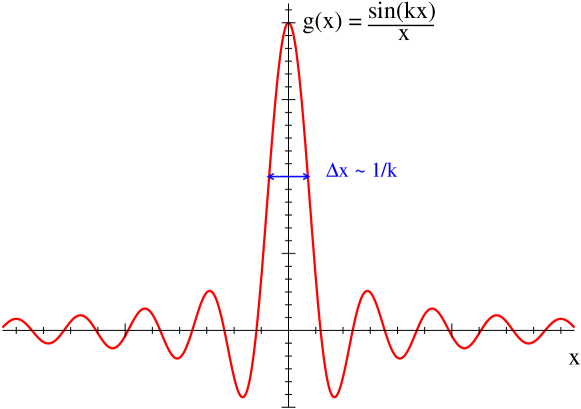
Figure 1: Function $g(x)=\sin(kx)/x$

Large values of $\delta$ correspond to small values of neutrino energy $E$ (see eq. (3)), therefore, the smaller the neutrino energy, the shorter the coordinate scale on which the Earth density profile can be probed. This may look somewhat counter-intuitive; however, one should remember that we are probing the Earth density distribution with neutrino oscillations rather than with direct neutrino-matter interactions. The smaller the neutrino energy, the shorter the oscillation length, and so the finer the density structures that can be probed. In future low-energy solar neutrino experiments, neutrinos of energies as small as a hundred keV to 1 MeV can probably be detected Raghavan , Ejiri:1999rk , LOWE ; this would correspond to $\delta_{max}\simeq(2\div 20)\times 10^{-11}$ eV, or $\Delta x\sim\pi/\delta_{max}\simeq(3\div 30)$ km, which is a very good coordinate resolution . For the neutrino path lengths $L\gtrsim 100$ km one finds $\delta_{max}L\gtrsim(10\div 100)$, i.e. the condition $\delta_{max}L\gg 1$ can be easily met.

At the same time, as we have already mentioned, having a sufficiently small $\delta_{min}$ may be a fundamental problem. There are two reasons for that. First, small $\delta_{min}$ implies large neutrino energies, and there are upper limits to the available neutrino energies. The spectrum of solar neutrinos extends up to 15 MeV ($hep$ neutrinos have slightly higher energies, but their flux is very small); the average energy of supernova neutrinos is $\sim 20$ MeV Keil:2002in . Yet, this problem can to some extent be alleviated, at least in principle. It might be possible to measure the Earth matter effect for supernova neutrinos of energies up to $\sim 100$ MeV, which are on the high-energy tail of the spectrum, but still not too far from the mean energy. Thus, for a nearby supernova and large enough detectors one can probably have sufficient statistics.

The second obstacle is of more fundamental nature. Our expressions (2) and (5) are only valid in the approximation $V/2\delta\ll 1$, which may break down for too small $\delta_{min}$. This gives a lower limit on the values of $\delta_{min}$ one can use, depending on the accuracy of the reconstructed potential one wants to achieve. In principle, one could attempt at deriving a more general expression for $f(\delta)$, not relying on the approximation $V/2\delta\ll 1$; in particular, it is fairly easy to study the opposite case $V/2\delta\gg 1$. However, for $V\gtrsim 2\delta$ the expression for $f(\delta)$ does not have a simple dependence on the potential $V(x)$, and solving the inverse problem of neutrino oscillations becomes a difficult task.

For an estimate of the constraint on $\delta_{min}$ imposed by the condition of small $V/2\delta$, let us require $V/2\delta_{min}<1/5$. For the matter density in the upper mantle of the Earth, $\rho\simeq 3$ g/cm³, this gives $\delta_{min}\gtrsim 2.8\times 10^{-13}$ eV, which for $\Delta m_{21}^{2}\simeq 7.9\times 10^{-5}$ eV² leads to $E_{max}\lesssim 70$ MeV. For neutrinos passing through the core of the Earth, the constraints on $\delta_{min}$ and $E_{max}$ will be a factor of 3 – 4 more stringent.

Let us now estimate the magnitude of $\delta_{min}L$ corresponding to $L\simeq 300$ km, which is a representative value of neutrino potholing inside the Earth, satisfying condition (14). For solar neutrinos ($E_{max}\simeq 15$ MeV) we find $\delta_{min}L\simeq 2$, while for supernova neutrinos, taking $E_{max}\simeq 70$ MeV, we obtain $\delta_{min}L\simeq 0.43$. Thus, except for very small values of $L$, we have to deal with situations when $\delta_{min}L\gtrsim 1$.

How large is the error introduced by non-vanishing $\delta_{min}$ in the reconstruction of the density profile $V(x)$? To study that, let us consider the integral of the type (6) with the finite lower integration limit $\delta_{min}=L^{-1}$. In fig. 2 the lowest curve gives the result of such a calculation for the step-function density profile (shown by the dashed line) and $\delta_{max}=300L^{-1}$. One can see several interesting features of the result. First, the deviation from the exact profile is relatively small near the detector ($x\simeq L$), but reaches about a factor of three far from it ($x\simeq 0$). Second, despite a significant deviation from the exact profile $V(x)$, the positions and the magnitudes of the jumps in $V(x)$ are reproduced very accurately. Both these features can be easily understood (see sections 4.2 and 4.2.2 below).

Thus, we have seen that the error in the reconstructed profile due to the lack of the knowledge of the Earth matter effect in the domain of low $\delta$ (high energies) can be quite substantial. We shall show now how this problem can be cured by invoking simple iteration procedures.

4.2 Iteration procedure I

Let us study the effect of non-vanishing $\delta_{min}$ in more detail. In order to do so, we consider the limit $\delta_{max}\to\infty$, which is justified by the preceding discussion. From eq. (15) one then readily finds

$$V(x)=\frac{4}{\pi}\int_{\delta_{min}}^{\infty}f(\delta)\sin 2\delta(L-x)d\delta+\frac{1}{\pi}\int_{0}^{L}V(y)F(x,y;2\delta_{min})dy\,,$$ (16)

where the function $F(x,y;k)$ is defined as

$$F(x,y;k)=\frac{\sin k(x-y)}{x-y}-\frac{\sin k(2L-x-y)}{2L-x-y}\,.$$ (17)

It is symmetric with respect to its first two arguments: $F(x,y;k)=F(y,x;k)$.

Equation (16) is exact provided that eq. (5) is exact. By comparing it with eq. (6), we find that the second integral in (16) can be considered as compensating for an error introduced in eq. (6) by having a non-zero lower limit in the integral over $\delta$. However, this compensating integral cannot be calculated directly because it contains the unknown potential $V(x)$. Thus, we have traded one unknown quantity – the function $f(\delta)$ in the domain $\delta<\delta_{min}$ – for another. At first sight, this does not do us any good. This is, however, incorrect: eq. (16) allows a simple iterative solution.

We first note that in the limit $\delta_{min}\to 0$ the second integral in eq. (16) disappears, while the first one yields $V(x)$. Therefore, for not too large values of $\delta_{min}$ the first term in (16) is expected to give a reasonable first approximation to $V(x)$. One can then use the result in the second integral to obtain the next approximation to $V(x)$, and so on. Thus, we define

$$V_{0}(x) = \frac{4}{\pi}\int_{\delta_{min}}^{\infty}f(\delta)\sin 2\delta(L-x)d\delta\,,$$ (18)

$$I_{0}(x) = \frac{1}{\pi}\int_{0}^{L}V_{0}(y)F(x,y;2\delta_{min})dy\,,\qquad\quad V_{1}(x)=V_{0}(x)+I_{0}(x)\,,$$

$$\dots\dots$$

$$I_{n-1}(x) = \frac{1}{\pi}\int_{0}^{L}V_{n-1}(y)F(x,y;2\delta_{min})dy\,,\qquad\quad\!\!V_{n}(x)=V_{0}(x)+I_{n-1}(x)\,.$$ (20)

This gives a sequence of potentials $V_{0}(x),\,V_{1}(x),\dots,\,V_{n}(x),\dots$ which, for small enough $\delta_{min}$, converges to $V(x)$. It should be noted that, while the exact eq. (16) is independent of $\delta_{min}$, our iteration procedure involves the approximate potentials and so depends on it. The smaller the chosen value of $\delta_{min}$, the faster the convergence of $V_{n}(x)$ to $V(x)$; for $\delta_{min}$ exceeding some critical value (which in general depends on the profile $N_{e}(x)$) the iteration procedure fails.

This is illustrated in figs. 2 - 4. In fig. 2 we show the potential $V(x)$ for the step-function model of the Earth density profile, along with the zeroth-order reconstructed potential $V_{0}(x)$ and the results of the first, second and fourth iterations $V_{1}(x)$, $V_{2}(x)$ and $V_{4}(x)$ ($V_{3}(x)$ is not shown in order to avoid crowding the figure). The calculations were performed for $\delta_{min}=L^{-1}$, $\delta_{max}=300L^{-1}$. One can see that already the fourth iteration gives an excellent agreement with the exact potential. We have checked that for $\delta_{min}\ll L^{-1}$ already the zeroth-approximation potential $V_{0}(x)$ gives a very good accuracy (see also section 4.2.2). The wiggliness of the reconstructed potentials in fig. 2 is due to the finiteness of $\delta_{max}$; with increasing $\delta_{max}$ it decreases.

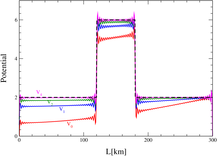
Figure 2: Step-function potential $V(x)$ (dashed line), zeroth order reconstructed potential $V_{0}(x)$ and the results of the first, second and fourth iterations $V_{1}(x)$, $V_{2}(x)$ and $V_{4}(x)$. The vertical scale is that of the corresponding matter density in g/cm³, assuming $Y_{e}=0.5$ and $\theta_{13}=0$. The following values of the parameters were chosen: $\delta_{min}=L^{-1}$, $\delta_{max}=300L^{-1}$.

If $\delta_{min}$ exceeds the critical value (which for the chosen profile is approximately equal to $2.4L^{-1}$ ), the successive iterations, instead of approaching the true potential, yield the potentials which more and more deviate from it. Thus, in this case the iteration procedure fails.

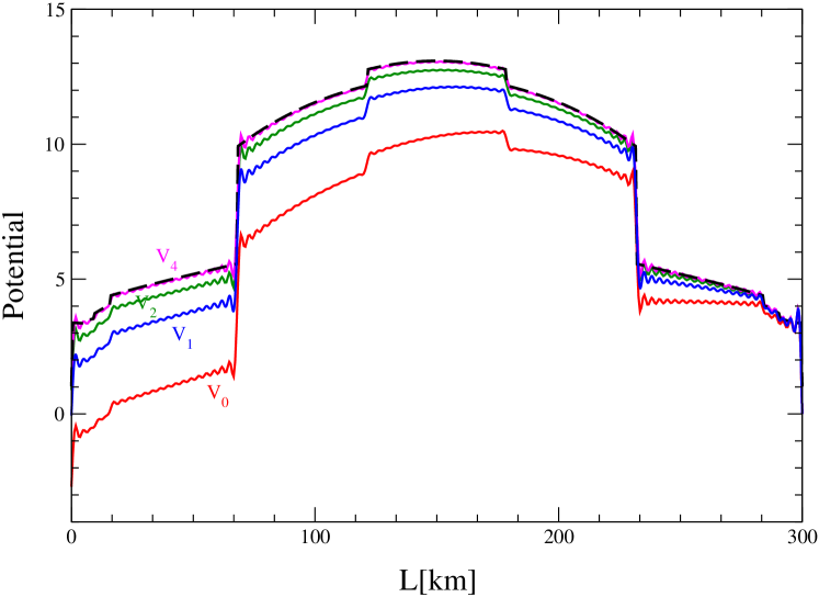
Figure 3: Same as in fig.2, but for PREM-like profile (shown by dashed line),

The iteration procedure works very well not only for simple profiles like the step-function profile in fig. 2, but also for more complicated ones. This is demonstrated in fig. 3, which is similar to fig. 2, but was plotted for the PREM-like density profile of the Earth Dziewonski:xy . It should be stressed that this profile was used in fig. 3 for illustrative purposes only, since, in the form we used it, it is a realistic Earth density profile for $L=2R_{\oplus}\simeq 12742$ km and not for $L=300$ km (for which the Earth density is actually better approximated by the step-function profile of fig. 2). Fig. 4 is similar to figs. 2 and 3, but was produced for an asymmetric Earth density profile (shown by the dashed line). It clearly demonstrates that asymmetric profiles can also be reconstructed very well, and so the inhomogeneities of matter distribution in the Earth can be studied by the method under consideration.

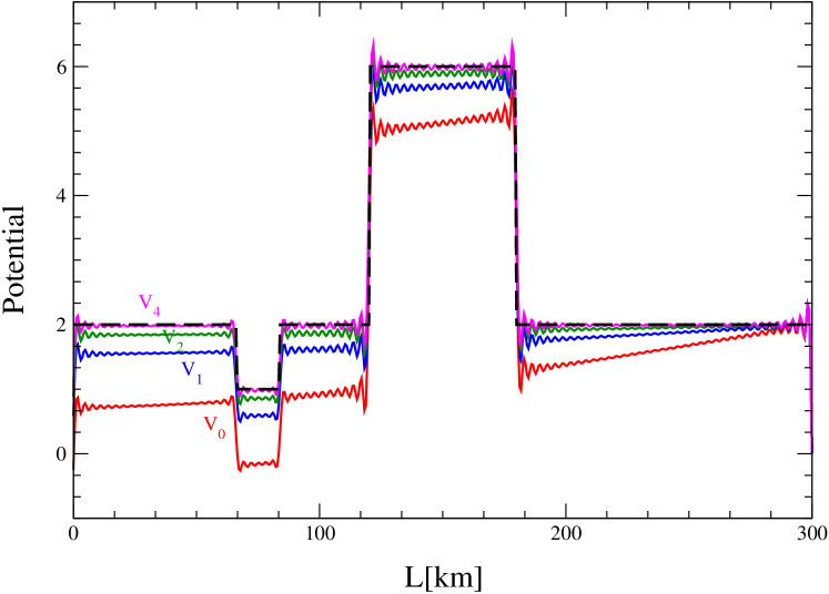
Figure 4: Same as in fig. 2, but for asymmetric step-function potential (dashed line).

Finally, we note that if $\delta_{max}L\gg 1$ but still not very large, one can devise an iterative procedure correcting for the corresponding error in the reconstructed potential (see Appendix A).

4.2.1 Convergence properties of iterations

We shall now discuss some properties of the iteration procedure (18) – (20). First, we note that the function $F(x,y;2\delta_{min})$ is positive definite for all $0<x,y<L$ provided that $\delta_{min}<2.246L^{-1}$ (see Appendix B for the proof). One can then show that for

$$\delta_{max}\to\infty\leavevmode\nobreak\ \leavevmode\nobreak\ \leavevmode\nobreak\ \mbox{and}\leavevmode\nobreak\ \leavevmode\nobreak\ \leavevmode\nobreak\ \delta_{min}<{\rm min}\{2.246L^{-1},\,\delta_{1}\}\,,$$ (21)

where $\delta_{1}$ will be defined shortly, the following string of inequalities is satisfied:

$$V_{0}(x)<V_{1}(x)<V_{2}(x)<...<V(x)\,.$$ (22)

This can be proven by induction. Consider first eq. (16). From the positivity of $V(x)$ and $F(x,y;2\delta_{min})$ it follows that the second integral in (16) (which we denote $I(x))$ is positive, and so the first integral, which is the zeroth-approximation potential $V_{0}(x)$, satisfies $V_{0}(x)<V(x)$. Generally, the larger $\delta_{min}$, the smaller $V_{0}(x)$; for large enough $\delta_{min}$ the potential $V_{0}(x)$ may even become negative for some values of $x$ in the interval $[0,\,L]$. However, if $\delta_{min}$ does not exceed certain limiting value $\delta_{1}$ (which we assume), the integral $I_{0}(x)$ defined in eq. (4.2) will still be positive. It is this limiting value $\delta_{1}$ that appears in eq. (21). From the definition of the integral $I_{0}(x)$ and the obtained condition $V_{0}(x)<V(x)$ we then find $0<I_{0}(x)<I(x)$. Therefore $V_{1}(x)=V_{0}(x)+I_{0}(x)$ satisfies $V_{0}(x)<V_{1}(x)<V(x)$. Then, from the definition of $I_{1}(x)$ we find $I_{0}(x)<I_{1}(x)<I(x)$, so that $V_{2}(x)=V_{0}(x)+I_{1}(x)$ satisfies $V_{1}(x)<V_{2}(x)<V(x)$. Continuing this procedure, we arrive at eq. (22).

Thus, under the conditions of eq. (21), each iteration produces the potential which is larger than that of the previous iteration. The potentials $V_{n}(x)$ approach the exact potential $V(x)$ from below and never exceed it. This is well illustrated by figs. 2 - 4 (we recall that the wiggliness of the curves disappears in the limit $\delta_{max}\to\infty$). Conditions (21) are thus sufficient for the convergence of the iteration procedure .

How can one estimate the critical value of $\delta_{min}$ above which the iteration procedure would diverge? From the preceding discussion it follows that the convergence of the iterations to the exact potential relies on the positivity of the “correction terms” $I_{n}(x)$. For values $\delta_{min}>\delta_{1}$ the integral $I_{0}(x)$ will become negative for some values of $x$ in the interval $[0,\,L]$, and so for those values of $x$ the potential $V_{1}(x)$ will deviate from $V(x)$ more than $V_{0}(x)$ does. If this propagates into the further iterations, the iteration procedure would fail. However, it is possible that even if some $I_{k}(x)$ are not positive definite, higher-order correction integrals $I_{n}(x)$ with $n>k$ are. In this case the iteration procedure would still be convergent.

In practice, it is difficult to determine the critical value of $\delta_{min}$ precisely. The closer (from below) $\delta_{min}$ to its critical value $\delta_{crit}$, the larger the number of iterations which is necessary to achieve a given accuracy of the reconstructed potential. Therefore, with $\delta_{min}$ approaching $\delta_{crit}$ it becomes more and more difficult to check if the procedure would converge. In addition, for $\delta_{min}$ close to $\delta_{crit}$ the behaviour of the iteration potentials $V_{n}(x)$ with increasing $n$ does not depend much on whether $\delta_{min}<\delta_{crit}$ or $\delta_{min}>\delta_{crit}$, so that it is difficult to decide if the critical value has already been exceeded. It is therefore reasonable to adopt some “practical” definition of $\delta_{crit}$, for example, as a value of $\delta_{min}$ for which the number of iterations necessary to reach a 10% accuracy of the reconstructed potential reaches 100. For all the density profiles that we studied this value turned out to be $\delta_{crit}\simeq 2.4L^{-1}$. We elaborate further on the convergence of the iterations in the next subsection.

Let us now return to the question of why the zeroth order potential $V_{0}(x)$ correctly reproduces the positions and magnitudes of the jumps in the exact potential $V(x)$. In eq. (16) (which is exact in the linear regime), the second term on the right-hand side is the integral over $y$ of the product of the continuous function $F(x,y;2\delta_{min})$ and the exact potential $V(y)$, which may have discontinuities, but no $\delta$-function type singularities. Hence, this integral is a continuous function of $x$. This immediately means that all possible jumps in $V(x)$ are contained in the first integral in eq. (16), i.e. $V_{0}(x)$.

4.2.2 The limit of small $\delta_{min}L$

It is very instructive to consider the iteration procedure in the limit $\delta_{min}L\ll 1$. Since $x,y\leq L$, the expression for $F(x,y;2\delta_{min})$ in this case simplifies to

$$F(x,y;2\delta_{min})\simeq\frac{16}{3}\,\delta_{min}^{3}\,(L-x)(L-y)\,.$$ (23)

Then from eq. (20) we find a very simple result:

$$I_{n}(x)\simeq\frac{16}{3\pi}\,\delta_{min}^{3}\,(L-x)\int_{0}^{L}V_{n}(y)(L-y)dy\,.$$ (24)

It means that the “correction terms” $I_{n}(x)$, which compensate for $\delta_{min}\neq 0$ in the inverse Fourier transformation, have a very simple coordinate dependence $\propto(L-x)$ for all $n$ and scale with $\delta_{min}L$ as $(\delta_{min}L)^{3}$. The same is true for the “exact” correction term $I(x)$ (the second integral in eq. (16)), which is obtained from eq. (24) by replacing in the integrand $V_{n}(y)$ by the exact potential $V(y)$. The approximately linear coordinate dependence of the deviation of the iteration potentials from the exact one can be seen even for $\delta_{min}L\sim 1$ (see figs. 2 - 4). It explains, in particular, why the deviations of $V_{n}(x)$ from the exact potential are small at $x\simeq L$ and largest at $x=0$.

Using eqs. (20) and (23), it is easy to show by induction that in the limit $\delta_{min}L\ll 1$

$$I_{n}(x)\simeq\frac{3}{2}\,v_{0}\left(\frac{16}{9\pi}\,\delta_{min}^{3}L^{3}\right)\left[1-\left(\frac{16}{9\pi}\,\delta_{min}^{3}L^{3}\right)^{n+1}\right]\,\frac{L-x}{L}\,,$$ (25)

$$V_{n}(x)\simeq V(x)-\frac{3}{2}v_{0}\left(\frac{16}{9\pi}\,\delta_{min}^{3}L^{3}\right)^{n+1}\frac{L-x}{L}\,,\leavevmode\nobreak\ \leavevmode\nobreak\ \leavevmode\nobreak\ \leavevmode\nobreak\ \leavevmode\nobreak\ \leavevmode\nobreak\ \leavevmode\nobreak\ \leavevmode\nobreak\ \leavevmode\nobreak\ \leavevmode\nobreak\ \leavevmode\nobreak\ \leavevmode\nobreak\ \leavevmode\nobreak\ \leavevmode\nobreak\ \leavevmode\nobreak\ \leavevmode\nobreak\ \leavevmode\nobreak\ \leavevmode\nobreak\$$ (26)

where the constant $v_{0}$ is defined as

$$v_{0}=\frac{2}{L^{2}}\int_{0}^{L}V(y)(L-y)dy\,.$$ (27)

Note that these equations are in accord with eq. (24). In the case of matter of constant density $V(x)=C_{0}=const$, one has $v_{0}=C_{0}$, and eq. (26) takes an especially simple form.

From eq. (26) it follows that for $\delta_{min}L\ll 1$ the deviation of the $n$th-iteration potential $V_{n}(x)$ from the exact one scales as $[(16/9\pi)\,\delta_{min}^{3}L^{3}]^{n+1}$, i.e. the convergence of $V_{n}(x)$ to the exact potential is very fast.

Although eqs. (25) and (26) were obtained for $\delta_{min}L\ll 1$, one can expect that they give correct order of magnitude estimates even for $\delta_{min}L\sim 1$. This allows one to estimate the number of iterations which is necessary to achieve a given accuracy of the reconstructed potential in the whole range $\delta_{min}\leq\delta_{crit}$. First, from eq. (26) we find that in the case under consideration the critical value of $\delta_{min}$, above which the iteration procedure diverges, is $\delta_{crit}=(9\pi/16)^{1/3}L^{-1}$, so that (26) can be rewritten as

$$V_{n}(x)=V(x)-(3v_{0}/2)(\delta_{min}/\delta_{crit})^{3(n+1)}(L-x)/L\,.$$ (28)

Assume now that we want the relative error in the reconstructed potential (which we define here as $|V(x)-V_{n}(x)|/v_{0}$) to be below $\varepsilon$. Then from (28) we find that the necessary number of iterations is

$$n\simeq\frac{\ln(2\varepsilon/3)}{3\ln(\delta_{min}/\delta_{crit})}-1\,.$$ (29)

As an example, take $\varepsilon=0.01$. Then for $\delta_{min}/\delta_{crit}=0.3$ already the zeroth-approximation potential $V_{0}(x)$ has the desired accuracy; for $\delta_{min}/\delta_{crit}=0.9$ eq. (29) gives $n\simeq 15$, for $\delta_{min}/\delta_{crit}=0.99$ it gives $n\simeq 165$, and in the limit $\delta_{min}\to\delta_{crit}$ one finds $n\to\infty$, as expected. It should be remembered, however, that for $\delta_{min}/\delta_{crit}\sim 1$ eq. (29) gives only a rough estimate of the necessary number of iterations because eq. (28) was obtained in the limit $\delta_{min}L\ll 1$, which essentially coincides with $\delta_{min}/\delta_{crit}\ll 1$.

We have considered in this subsection the reconstruction of the potential $V(x)$ in the limit of small $\delta_{min}L$ iteratively only in order to illustrate some general features of the iteration procedure. In fact, for $\delta_{min}L\ll 1$ it is easy to find the closed-form solution of eq. (16) . Indeed, since in this case $I(x)\propto(L-x)$, the potential $V(x)$ can be written as $V(x)=V_{0}(x)+C_{1}(L-x)$ with $C_{1}$ a constant. Substituting this into eq. (16), one readily determines $C_{1}$, which gives

$$V(x)\simeq V_{0}(x)+C_{2}\frac{\frac{16}{3\pi}\delta_{min}^{3}L^{3}}{1-\frac{16}{9\pi}\delta_{min}^{3}L^{3}}\,\frac{L-x}{L}\,$$ (30)

with

$$C_{2}=\frac{1}{L^{2}}\int_{0}^{L}V_{0}(y)(L-y)dy\,.$$ (31)

Since the function $V_{0}(x)$ is known, the problem is solved.

4.3 Iteration procedure II

In the iteration procedure considered in section 4.2 we assumed that nothing is known a priori about the Earth density profile, and the only experimental data available were the neutrino data. If some (even very rough) prior knowledge of the matter density distribution inside the Earth exists, one can employ a much better and faster iteration procedure to reconstruct the Earth density profile. As an example, we consider here the case when the average matter density along the neutrino path is known. The corresponding average potential

$$\overline{V}=\frac{1}{L}\int_{0}^{L}V(x)\,dx\,.$$ (32)

is therefore known as well. The new iteration procedure is again described by eqs. (4.2) - (20), but the zeroth order approximation potential is now $V_{0}(x)=\overline{V}=const$. In fig. 5 we plot this potential (horizontal line) and the first iteration potential $V_{1}(x)$ for the asymmetric step-function profile of fig. 4 (shown by the dashed line). One can see that, although $V_{0}$ is completely structureless, already the first iteration reproduces the exact profile extremely well. This should be compared with the results of iteration scheme I, for which only the fourth iteration gives similar accuracy (see fig. 4).

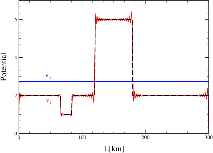
Figure 5: Asymmetric step-function profile (dashed line), zeroth approximation potential $V_{0}(x)=\overline{V}$ and first order iteration potential $V_{1}(x)$. Vertical scale and values of parameters are the same as in fig. 2.

To understand why this iteration scheme works so well, it is instructive to consider it in the limit $\delta_{min}L\ll 1$. First, we note that for an arbitrary $\delta_{min}$ and $n\geq 1$ eqs. (16) and (20) yield

$$V(x)-V_{n}(x)=\frac{1}{\pi}\int_{0}^{L}[V(y)-V_{n-1}(y)]F(x,y;2\delta_{min})dy\,.$$ (33)

In the limit $\delta_{min}L\ll 1$, the function $F(x,y;2\delta_{min})$ is given by (23); substituting this into (33), for $n=1$ we find

$$V(x)-V_{1}(x)\simeq\left(\frac{8}{3\pi}\,\delta_{min}^{3}L^{3}\right)\frac{L-x}{L}(v_{0}-\overline{V})\,,\leavevmode\nobreak\ \leavevmode\nobreak\ \leavevmode\nobreak\ \leavevmode\nobreak\ \leavevmode\nobreak\ \leavevmode\nobreak\ \leavevmode\nobreak\ \leavevmode\nobreak\ \leavevmode\nobreak\ \leavevmode\nobreak\ \leavevmode\nobreak\ \leavevmode\nobreak\ \leavevmode\nobreak\ \leavevmode\nobreak\ \leavevmode\nobreak\ \leavevmode\nobreak\ \leavevmode\nobreak\ \leavevmode\nobreak\$$ (34)

where $v_{0}$ was defined in (27). For $n$th iteration ($n\geq 1$) we find by induction

$$V(x)-V_{n}(x)\simeq\frac{3}{2}\left(\frac{16}{9\pi}\,\delta_{min}^{3}\leavevmode\nobreak\ L^{3}\right)^{n}\frac{L-x}{L}(v_{0}-\overline{V})\,.\leavevmode\nobreak\ \leavevmode\nobreak\ \leavevmode\nobreak\ \leavevmode\nobreak\ \leavevmode\nobreak\ \leavevmode\nobreak\ \leavevmode\nobreak\ \leavevmode\nobreak\ \leavevmode\nobreak\ \leavevmode\nobreak\ \leavevmode\nobreak\ \leavevmode\nobreak\ \leavevmode\nobreak\ \leavevmode\nobreak\ \leavevmode\nobreak\ \leavevmode\nobreak\ \leavevmode\nobreak\ \leavevmode\nobreak\$$ (35)

Comparing this with (26), we find that in iteration scheme II the difference $V(x)-V_{n}(x)$ contains one less power of $[(16/9\pi)\,\delta_{min}^{3}L^{3}$], but is proportional to $v_{0}-\overline{V}$ rather than to $v_{0}$. We shall show now that for symmetric density profiles ($V(x)=V(L-x)$) the difference $v_{0}-\overline{V}$ vanishes, and therefore already the first iteration reproduces the exact profile. Indeed, from eqs. (27) and (32) we have

$$v_{0}-\overline{V}=\frac{1}{L^{2}}\int_{0}^{L}V(y)[2(L-y)-L]\,dy=\frac{2}{L^{2}}\int_{-L/2}^{L/2}V(z)z\,dy\,,$$ (36)

where in the last integral we changed the integration variable to $z=L/2-y$. For symmetric density profiles, $V(z)$ is an even function of $z$, and the integral in (36) vanishes.

What if the density profile is not symmetric? In that case one can write $V(z)=V_{s}(z)+V_{a}(z)$, where $V_{s}(z)$ and $V_{a}(z)$ are the symmetric and antisymmetric parts of $V(z)$. The symmetric part $V_{s}(z)$ does not contribute to the integral in (36), whereas the contribution of $V_{a}(z)$ is small because the inhomogeneities of the Earth density distribution, responsible for $V_{a}$, occur on short coordinate scales . Thus, in scheme II, even for asymmetric density profiles the first iteration gives a very good approximation to the exact profile (see fig. 5).

It should be noted that, while the above discussion referred to the case $\delta_{min}L\ll 1$, fig. 5 actually corresponds to $\delta_{min}L=1$. However, our consideration approximately applies to that case as well. For $\delta_{min}L\sim 1$, the integrand of the driving term for the second iteration in scheme II will be proportional, instead of $V(y)(L/2-y)$, to the product of $V(y)$ and the function $[F(x,y;2\delta_{min})-(1/L)\int_{0}^{L}F(x,x^{\prime};2\delta_{min})dx^{\prime}]$. This function, though not exactly antisymmetric with respect to $y\to L-y$, is almost antisymmetric (for all $x\in[0,L]$). This explains why iteration scheme II works so well even in the case $\delta_{min}L\sim 1$.

5 Non-linear regime

Our previous discussion of the reconstruction of the Earth density profile was based on the simple formula (5) for the function $f(\delta)$, which was derived under the assumptions (13). The second of these conditions led to a rather stringent upper limit on the neutrino path lengths in the Earth (14), or $L\lesssim 300$ km. In order to be able to reconstruct the potential $V(x)$ over larger distances, one has to employ an inversion procedure based on the more accurate expression (2), which only requires the first condition in (13) for its validity. Let us now discuss this improved expression.

Since the function $\omega(x)$ in eq. (2) depends on $V(x)$, we face a non-linear problem now. The first condition in (13) and the non-linearity condition $VL\gtrsim 1$ imply $\delta_{min}L\gg 1$. This, in turn, means that the matter density profile cannot be found by invoking an iteration procedure , and one should resort to different methods of solving eq. (2). The simplest possibility would be to discretize the problem and reduce the non-linear integral equation (2) to a set of non-linear algebraic equations, which can then be solved numerically. However, eq. (2) is a non-linear Fredholm integral equation of the first kind , and equations of this type are notoriously difficult to solve. Integral equations of the first kind belong to the so-called ill-posed problems: their solutions are very unstable, and to arrive at a reliable result one has to invoke special regularization procedures. For linear integral equations, such procedures are well developed (see section 6.2 and Appendices C and D for more details); however, no universal regularization techniques exist for non-linear integral equations of the first kind. The situation is further complicated by the fact that for $\delta_{min}L\gg 1$ the potential $V(x)$ enters into the integrand of eq. (2.2) being multiplied by a fast oscillating function of the coordinate. All this makes the non-linear regime of the inverse problem of neutrino oscillations in matter very difficult to explore. This regime therefore requires a dedicated study, which goes beyond the scope of the present paper.

6 Experimental considerations

Up to now we ignored completely the experimental questions, such as the effects of the errors in experimental data and of finite energy resolution of neutrino detectors on the accuracy of the reconstructed matter density distributions. We now turn to these issues. We shall discuss here only the linear regime of the density profile reconstruction; the experimental questions pertaining to the non-linear regime will be considered elsewhere.

6.1 Effects of experimental errors

For solar neutrinos, the night-day asymmetry of the signal can be written as Akhmedov:2004rq

$$A_{ND}=2\frac{N-D}{N+D}\simeq-c_{13}^{2}\left[\frac{\sin^{2}2\theta_{12}\,\overline{\cos 2\hat{\theta}_{12}}}{1+\cos 2\theta_{12}\,\overline{\cos 2\hat{\theta}_{12}}}\right](f(\delta)/c_{13}^{2})\,,$$ (37)

where $\overline{\cos 2\hat{\theta}_{12}}$ is cosine of twice the effective 1-2 mixing angle in matter, averaged over the neutrino production coordinate inside the Sun Blennow:2003xw . The quantity $f(\delta)/c_{13}^{2}$ is independent of $c_{13}^{2}$ in the linear regime (see eqs. (5) and (4)). Thus, the relative error of the experimentally determined value of $f(\delta)/c_{13}^{2}$ is the sum of the relative errors of $A_{ND}$, $c_{13}^{2}$ and of the $\theta_{12}$ - dependent expression in the square brackets in eq. (37). The dependence of the latter on the error of $\theta_{12}$ is somewhat involved (mainly, because of the $\theta_{12}$ dependence of the effective mixing angle in matter $\hat{\theta}_{12}$). It can be approximated by

$$\epsilon_{\theta_{12}}\simeq\left[1.74-\frac{1.83\,[1-(0.4-V_{av}/2\delta)^{2}]}{(0.4-V_{av}/2\delta)[1+0.4(0.4-V_{av}/2\delta)]}\right]\Delta\theta_{12}\,,$$ (38)

where $V_{av}$ is the averaged over the neutrino production region value of the matter-induced neutrino potential in the Sun. The values of $V_{av}$ for various components of the solar neutrino spectrum can be found in table 1 of ref. deHolanda:2004fd .

The next question is how the error in the experimentally determined quantity $f(\delta)/c_{13}^{2}$ affects the accuracy of the reconstructed electron number density profile $N_{e}(x)$. Since, in the linear regime, to obtain a solution we invoke an iteration procedure, one might expect that the corresponding errors in the reconstructed density profile would accumulate with increasing iteration order. This is, however, not the case: at each iteration, the relative error of the solution is the same as the relative error of $f(\delta)/c_{13}^{2}$, and the same applies to the exact profile $N_{e}(x)$. This follows from the fact that each iteration profile and the exact solution depend linearly on $f(\delta)/c_{13}^{2}$, which is a consequence of the linearity of eq. (16).

The main contribution to the error of $f(\delta)/c_{13}^{2}$ (and thus, of the reconstructed electron number density profile) is expected to come from the error in $A_{ND}$, which is by far the largest one (at the moment, more than 100%). Therefore, an accurate reconstruction of the matter density distribution inside the Earth would require very large detectors, capable of measuring the solar neutrino day-night effect with an accuracy commensurate with the desired accuracy of the matter density reconstruction.

From eqs. (2) and (3) it follows that the errors in the parameter $\Delta m_{21}^{2}$ and in the energy scale of neutrino detectors go linearly to the shifts in the reconstructed coordinate.

6.2 Finite energy resolution of detectors

Let us consider now the effects of finite energy resolution of neutrino detectors. We shall be assuming that neutrinos are detected through a charged-current capture reaction, so that the energy of the emitted electron in the final state directly gives the energy of the incoming neutrino. The electron energy, however, is not exactly measured because of the finite energy resolution of the detector, characterized by the resolution function $R(T_{e},T_{e}^{\prime})$. Here $T_{e}$ and $T_{e}^{\prime}$ are the observed and true electron kinetic energies, respectively. Because of the one-to-one correspondence between the electron and neutrino energies, the resolution function can be written directly in terms of the “observed” and true neutrino energies. In our discussion it proved more convenient to use $\delta=\Delta m_{21}^{2}/4E$ instead of the neutrino energy $E$, therefore we will be considering the detector resolution functions expressed in terms of $\delta$ and $\delta^{\prime}$. In many cases the resolution function can be approximated by a Gaussian

$$R(\delta,\delta^{\prime})=\frac{1}{\sqrt{2\pi}\,\sigma(\delta)}\,\exp\left\{-\frac{(\delta-\delta^{\prime})^{2}}{2\sigma^{2}(\delta)}\right\}$$ (39)

with $\delta$-dependent width, e.g., $\sigma(\delta)=k_{0}\delta$ or $\sigma(\delta)=k_{0}\sqrt{\delta_{max}\delta}$.

When finite energy resolution of detectors is taken into account, the function $f(\delta)$ in the expression for the Earth regeneration factor in eq. (1) has to be replaced by

$${\cal F}(\delta)=\int_{0}^{\infty}R(\delta,\delta^{\prime})f(\delta^{\prime})\,d\delta^{\prime}\,,$$ (40)

which describes the smoothing of $f(\delta)$ with the resolution function. In order to proceed with the density profile reconstruction, we have first to extract $f(\delta^{\prime})$ from the experimentally measured quantity ${\cal F}(\delta)$. Once this has been done, one can employ the procedures described in sections 4 or 5. Thus, instead of one-step inverse problem, we now have a two-step one.

6.2.1 Finite energy resolution effects on the Earth regeneration factor

Let us first discuss the physical effects of the finite energy resolution of detectors on the observed Earth matter effect. In ref. Ioannisian:2004jk it was shown that in the simplified case of the box-shaped resolution function with the energy width $\Delta E$, eq. (2) has to be replaced by

$${\cal F}(\delta)\simeq\int_{0}^{L}V(x)\frac{\sin\Delta(\delta)(L-x)}{\Delta(\delta)(L-x)}\sin\left[2\int\limits_{x}^{L}\!\omega(x^{\prime})\,dx^{\prime}\right]dx\,,$$ (41)

where $\Delta(\delta)$ is the resolution width in terms of $\delta$: $\Delta(\delta)=\delta\cdot(\Delta E/E)$. Eq. (41) differs from (2) by the extra factor $\sin\Delta(\delta)(L-x)/[\Delta(\delta)(L-x)]$ in the integrand. This factor equals unity when $\Delta(\delta)(L-x)=0$ (which corresponds to perfect energy resolution or $x=L$), and quickly decreases with increasing $\Delta(\delta)(L-x)$ (see fig. 1). Thus, finite energy resolution of detectors leads to an attenuation of the contributions to the Earth matter effect coming from the density structures which are far from the detector, the attenuation length (distance from the detector) being

$$l_{att}\leavevmode\nobreak\ \simeq\leavevmode\nobreak\ \frac{1}{\delta}\,\frac{E}{\Delta E}\leavevmode\nobreak\ =\leavevmode\nobreak\ \frac{1}{\pi}\,l_{osc}(E)\,\frac{E}{\Delta E}\,.$$ (42)

From eq. (42) it follows that for the attenuation to be negligible, i.e. for $l_{att}$ to exceed considerably $L$ for all energies of interest, one needs

$$\delta_{max}L\,\ll\frac{E}{\Delta E}\,.$$ (43)

This can be in conflict with the requirement of good coordinate resolution $\delta_{max}L\gg 1$, unless the energy resolution is extremely good. Thus, finite energy resolution worsens the coordinate resolution of the reconstruction procedure. If one completely ignores the fact that finite energy resolution of neutrino detectors modifies the observed matter effect and simply uses ${\cal F}(\delta)$ instead of $f(\delta)$ for the density profile reconstruction, then in the case when condition (43) is not satisfied it is essentially the finite energy resolution and not the value of $\delta_{max}$ that determines the coordinate resolution of the inversion procedure. Increasing $\delta_{max}$ beyond the limit (43) would not lead to any significant improvement of the coordinate resolution in that case.

Eq. (41) exhibits a power-law attenuation of the matter density structures far from the detector in the case of box-shaped energy resolution function. However, in a more realistic case of the Gaussian energy resolution, an even stronger (exponential) attenuation results. To show that, we first recall that the function ${\cal F}(\delta)$ is measured in a finite interval $\delta\in[\delta_{min},\delta_{max}]$. Although the integral in eq. (40) extends over the whole interval $0\leq\delta^{\prime}<\infty$, in fact the contributions to this integral coming from the domains of $\delta^{\prime}$ which are far outside the interval $[\delta_{min},\delta_{max}]$ are strongly suppressed because of the presence of the resolution function $R(\delta,\delta^{\prime})$ in the integrand. In particular, if $\delta_{min}$ exceeds a few widths of the Gaussian resolution function (39), one can formally extend the integration in eq. (40) to negative values of $\delta^{\prime}$ without affecting noticeably the value of the integral. Extending the integration to the interval $-\infty<\delta^{\prime}<\infty$, from eqs. (40), (39) and (2) one readily finds

$${\cal F}(\delta)\simeq\int_{0}^{L}V(x)\,e^{-2(L-x)^{2}\sigma^{2}(\delta)}\,\sin\left[2\int\limits_{x}^{L}\!\omega(x^{\prime})\,dx^{\prime}\right]dx\,.$$ (44)

6.2.2 Undoing the smoothing

We now turn to the question of how to reconstruct the electron number density profile of the Earth from the Earth regeneration factor in the presence of a well-known but finite energy resolution. As we already pointed out, if one ignores the fact the observed Earth regeneration factor is modified by the finite energy resolution of the detector and naively uses ${\cal F}(\delta)$ instead of $f(\delta)$ for the density profile reconstruction, the coordinate resolution of the reconstruction procedure will in general be very poor. We have checked numerically that for $\delta_{max}L\gtrsim 100$ and the energy resolution width $\Delta E/E=\Delta(\delta)/\delta$ exceeding 1%, the reconstructed profile differs sizeably from the true one. However, if the resolution function is well known, one can do a much better job: first, recover the function $f(\delta^{\prime})$ from the experimentally measured quantity ${\cal F}(\delta)$, and then reconstruct the Earth density profile from $f(\delta^{\prime})$. In other words, one could to some extent undo the smoothing of $f(\delta^{\prime})$ caused by the finite energy resolution of the neutrino detectors and described by eq. (40). This is similar to the procedures one has to invoke in various remote sensing problems (e.g., in medical tomography).

In principle, if the resolution function $R(\delta,\delta^{\prime})$ is exactly known and the function ${\cal F}(\delta)$ is precisely determined from the experiment, one could expect that the function $f(\delta^{\prime})$ can be exactly found from (40). This is, however, not the case. The point is that eq. (40) is a Fredholm integral equation of the first kind, which belongs to the class of ill-posed problems: small variations in ${\cal F}(\delta)$ can lead to very large changes in the reconstructed function $f(\delta^{\prime})$. To illustrate this, let us note that for any integrable $R(\delta,\delta^{\prime})$ and an arbitrary constant $A$

$$\lim_{k\to\infty}\,\int_{0}^{\infty}R(\delta,\delta^{\prime})\,A\sin(k\delta^{\prime})\,d\delta^{\prime}\leavevmode\nobreak\ =\leavevmode\nobreak\ 0\qquad\quad$$

by Riemann-Lebesgue lemma. Therefore, even for very large values of $A$, changing $f(\delta^{\prime})\to f(\delta^{\prime})+A\sin(k\delta^{\prime})$ practically does not modify the observable ${\cal F}(\delta)$ if $k$ is large enough. This means that small variations in ${\cal F}(\delta)$ correspond to very large high-frequency changes in the reconstructed function $f(\delta^{\prime})$. The solution does not depend continuously on the data, i.e. is highly unstable.

The function ${\cal F}(\delta)$ is always determined experimentally with some errors; the errors are drastically magnified in the process of solving eq. (40) for $f(\delta^{\prime})$. Even if one assumes ${\cal F}(\delta)$ to be exactly known, the rounding errors, which are inherent to any numerical calculation, would play the same role as the experimental errors and destabilize the solution. Therefore, straightforward methods of solving Fredholm integral equations of the first kind (such as discretization and reduction to a system of linear algebraic equations) do not work. One has to employ some regularization in order to suppress high-frequency noise in the solution.

There exist many regularization approaches for ill-posed problems and a vast literature on the subject. In our calculations we use two popular regularization schemes: the truncated singular value decomposition (TSVD) TSVD and the Backus-Gilbert (BG) method BG , LE , num , which are described in Appendices C and D, respectively. The results of calculations for the step-function density profile and the Gaussian detector resolution function (39) with 10% resolution ($k_{0}=0.1$) are presented in figs. 6 and 7. In these figures shown are the exact profile (dashed line) and the reconstructed profiles in the case of Gaussian resolution: the naive calculation, which used ${\cal F}(\delta)$ instead of $f(\delta^{\prime})$, is shown by the dash-dotted curve, while the results of the corresponding regularization approaches are shown by the solid curves. In the case of the TSVD regularization, the contributions of the singular values $\lambda_{i}\leq 10^{-10}$ were truncated (see Appendix C); in the BG approach, 1501-point calculation has been used. One can see from the figures that, while the naive calculation gives very poor reconstruction of the density profile far from the detector, undoing the smoothing caused by the finite energy resolution of the detectors improves the quality of the reconstruction drastically.

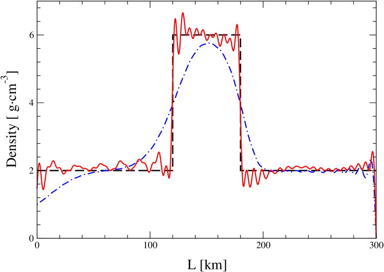
Figure 6: Density reconstruction for step-function density profile using TSVD method. The dashed line is the exact profile, the dash-dotted curve corresponds to a naive calculation using ${\cal F}(\delta)$ instead of $f(\delta^{\prime})$ for 10% Gaussian resolution, the solid curve is the result of TSVD regularization for Gaussian resolution, truncation at $\lambda_{i}\leq 10^{-10}$.

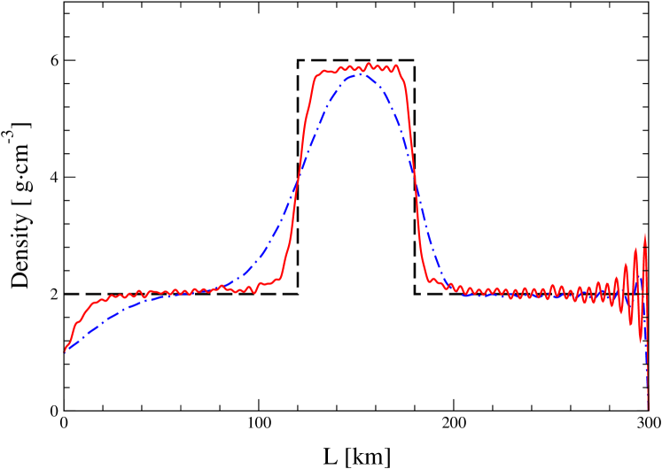
Figure 7: Same as in fig. 6, but for Backus-Gilbert method with $N=1501$ points.

Comparing figs. 6 and 7 one can see that the BG method gives in general more accurate reconstruction of the profile in the regions that are far from the ends of the neutrino trajectory in the Earth, whereas the TSVD method better reproduces the exact profile near these endpoints, $x\simeq 0$ and $x\simeq L$, and the jumps of the density (at the jumps, the TSVD curve is steeper than that of the BG approach). One can employ both these methods of data treating for the same set of experimental data and thus combine the advantages of each approach.

7 Discussion and outlook

We have developed a novel, direct approach to neutrino tomography of the Earth, based on a simple analytic formula for the Earth matter effect on oscillations of solar and supernova neutrinos inside the Earth. These neutrinos have a number of advantages over the accelerator neutrinos from the viewpoint of the tomography of the Earth. Apart from coming from a free neutrino source, they are sensitive to the Earth matter effects even if the distances they travel in the Earth are as short as $\sim 50$ - 100 km. In addition, they can be used for reconstructing asymmetric density profiles and thus are sensitive to short scale inhomogeneities of matter distribution in the Earth, as possibly relevant in prospection applications. Neutrino tomography allows the reconstruction of the electron number density of the Earth, i.e. is sensitive to its chemical composition. In this respect it can nicely complement geoseismological studies, which are based on the measurements of the spatial distributions of seismic wave velocities and can only probe the total density of the Earth’s matter, but not its chemical composition.

In the linear regime, which is valid for relatively short distances traveled by neutrinos in the Earth (up to several hundred km), the problem amounts to finding an inverse Fourier transform of the Earth regeneration factor. However, to perform this transformation, one needs to know the Earth regeneration factor in the whole infinite interval of neutrino energies $0\leq E<\infty$, whereas experimentally it can only be measured in a finite range $E_{min}\leq E\leq E_{max}$. Non-vanishing $E_{min}$ leads to a finite coordinate resolution $\Delta x\sim l_{osc}(E_{min})$ of the reconstruction procedure, while finite $E_{max}$ results in a systematic shift of the reconstructed profile compared to the true one.

Future experiments should be able to detect solar neutrinos with energies as small as $\sim 100$ keV, which means that a very good coordinate resolution can in principle be achieved; at the same time, finite $E_{max}$, i.e. the lack of knowledge of the Earth regeneration factor in the high energy domain, could potentially be a serious drawback for the neutrino tomography of the Earth. We have shown, however, that this ignorance of the Earth matter effect at high neutrino energies can be compensated for by making use of simple iterative procedures. We have developed two such iteration schemes, one of them not using any prior information about the Earth density profile, and the other assuming the average matter density along the neutrino path to be known. Both schemes give very good results, the second one leading to a faster convergence.

In order to reconstruct the Earth matter density profiles over the distances of geophysical interest, i.e. exceeding a few hundred km, one needs to solve a complex non-linear problem. It should be noted, however, that even in the linear regime ($L\lesssim\,$ a few hundred km) one can obtain very interesting information about the structure of the Earth’s crust and upper mantle. The maximal depth $d$ of the neutrino trajectory inside the Earth is

$$d=R_{\oplus}-\sqrt{R_{\oplus}^{2}-(L/2)^{2}}\,,$$ (45)

where $R_{\oplus}=6371$ km is the average radius of the Earth. For $L=300$ km this gives $d\simeq 1.8$ km, which could be quite sufficient, e.g., for minerals, oil and gas prospecting. Learning more about the large-scale structure of the Earth’s interior would require calculations in the non-linear regime.

There is a number of very interesting physics and mathematics issues related to the problem of neutrino tomography of the Earth, which still are to be explored. We have studied in detail the linear regime of the Earth density profile reconstruction; attacking the non-linear regime remains a challenge for future investigations. Another issue is recovering the true Earth regeneration factor, necessary for the inversion procedure, from the experimentally measured one, which is smoothed due to the finite energy resolution of the detector. Similar procedures are invoked in various remote sensing problems (e.g., in medical tomography, early vision, inverse problems of geo- and helioseismology, etc.). We have used two relatively simple methods of undoing the smoothing effects, the truncated singular value decomposition and the Backus-Gilbert method, and only in the linear regime. At the same time, there is a variety of other methods developed for solving problems of this kind; it would be interesting to study some of them in application to the neutrino tomography of the Earth, and also to consider the de-smoothing procedure in the non-linear regime.

Due to the rotation of the Earth, for a fixed position of the detector solar neutrinos will probe the Earth density distribution along a number of chords, ending at the detectors and spanning a segment inside the Earth. The size of the segment will depend on the geographic location of the detector. Because of the relatively low statistics, only density distributions averaged over certain angular bins of incoming neutrino directions will be probed. In order to reduce these averaging effects, i.e. to have small angular bins, one would need very large detectors and/or large overall detection time. Supernova explosions being one-shot events, the Earth tomography with supernova neutrinos will allow the density profile reconstruction only along a single neutrino path for each detector and each supernova, depending on the detector and supernova positions at the time the supernova neutrinos arrive at the Earth.

The accuracy of the reconstruction of the Earth matter density distribution will depend crucially on the accuracy of the experimental data – of the measured Earth regeneration factor and of the neutrino oscillation parameters. It will also depend on the accuracy of the reconstruction procedure itself. The largest error is expected to come from the errors in the measured Earth matter effect, mainly because this effect is rather small for solar and supernova neutrinos. To achieve a given accuracy of the density profile reconstruction, one should measure the Earth matter effect with similar or better accuracy. The present value of the night-day asymmetry of the solar neutrino signal, measured at Super-Kamiokande, is $2.1\%\pm 2.0\%(\rm{stat})\pm 1.3\%(\rm{syst})$ Smy:2003jf , i.e. the error constitutes more than 100%. This is certainly a very important limiting factor for the reconstruction method described here. Future megaton water Cherenkov detectors, such as UNO or Hyper-Kamiokande, are expected to reduce this error by a factor of 4 to 10; however, such detectors, unfortunately, are not very suitable for neutrino tomography of the Earth. The reason is that they are based on the $\nu e$ scattering process, in which the measured energy of the recoil electron gives only loose information on the energy of the incoming neutrino . Detectors based on charged-current neutrino capture reactions, such as LENS or MOON Raghavan , Ejiri:1999rk , LOWE , are probably more promising. It is not clear, however, whether sufficiently large (megaton or perhaps even tens of megaton scale) detectors of this kind can be constructed, and much work still has to be done to assess the feasibility of neutrino tomography of the Earth. In any case, studying the Earth’s interior with neutrinos is an exciting possibility, which can add yet another motivation for very large detectors of solar and supernova neutrinos.

Acknowledgements. The authors are grateful to G. Fiorentini and A. Yu. Smirnov for useful discussions. This work was supported by Spanish grant BFM2002-00345 and by the European Commission Human Potential Program RTN network MRTN-CT-2004-503369. The work of E.A. was partially supported by the sabbatical grant No. SAB2002-0069 of the Spanish MECD. M.A.T. is supported by the M.E.C.D. fellowship AP2000-1953.

Appendix A The case of not very large $\delta_{max}L$

If $\delta_{max}L\gg 1$ but still not very large, one can develop an iterative procedure correcting for the corresponding error in the reconstructed potential.

Let us add to and subtract from eq. (15) the corresponding integral from $\delta_{min}$ to $\delta_{0}$, where $\delta_{0}\gg\delta_{max}$ is a “numerical emulation of infinity”, i.e. a large number for which one can neglect the difference between $\sin(\delta_{0}x)/x$ and $\pi\delta(x)$ (e.g., $\delta_{0}=10^{3}L^{-1}$). This gives

$$V(x)\simeq\frac{4}{\pi}\int_{\delta_{min}}^{\delta_{max}}f(\delta)\sin 2\delta\,(L-x)\,d\delta\,+\frac{1}{\pi}\int_{0}^{L}V(y)\{F(x,y;2\delta_{min})\qquad\quad$$

$$+\,F(x,y;2\delta_{0})-F(x,y;2\delta_{max})\}\,dy\,.$$ (46)

If eq. (5) is exact, eq. (46) becomes exact in the limit $\delta_{0}\to\infty$. Note that the first term on the right hand side of (46) contains integration over $\delta$ from $\delta_{min}$ to $\delta_{max}$, and not from $\delta_{min}$ to $\infty$. Thus, it properly takes into account that the function $f(\delta)$ is only measured in the energy interval $E_{min}\leq E\leq E_{max}$ with $E_{min}\neq 0$.

Eq. (46) can now be solved by iterations, the procedure being quite analogous to the one used for solving eq. (16) in sections 4.2 or 4.3. If $\delta_{max}L$ is a very large number, the difference between the solutions of eqs. (16) and (46) is numerically insignificant, but it can be noticeable when $\delta_{max}L$ is not too large. In our calculation in the present paper we always use $\delta_{max}L\geq 100$, so that there is no need to solve the improved equation (46).

Appendix B Properties of $F(x,y;2\delta_{min})$

Let us prove that

$$F(x,y;2\delta_{min})>0\quad\mbox{for all}\quad 0<x,y<L\quad\mbox{and}\quad\delta_{min}<2.246L^{-1}\,.$$ (B1)

Indeed, the function $F(x,y;k)$ defined in eq. (17) can be written as $F(x,y;k)=g(x^{\prime}-y^{\prime})-g(x^{\prime}+y^{\prime})$, where $g(z)=\sin kz/z$, $x^{\prime}=L-x$, $y^{\prime}=L-y$. For positive $k$, the function $g(z)$ reaches its first minimum at $kz\simeq 4.493$ and is a decreasing function of $z$ for $0<kz<4.493$ (see fig. 1). Since $|x^{\prime}-y^{\prime}|\leq x^{\prime}+y^{\prime}$, $F(x,y;k)$ is positive for all $0<x,y<4.493/k$. Substituting $k=2\delta_{min}$ and requiring $0<x,y<L<4.493/2\delta_{min}$, one arrives at (B1).

Appendix C Truncated singular value decomposition (TSVD)

Any square-integrable function $R(\delta,\delta^{\prime})$ can be represented as TSVD

$$R(\delta,\delta^{\prime})\leavevmode\nobreak\ =\leavevmode\nobreak\ \sum_{i=1}^{\infty}\lambda_{i}\,u_{i}(\delta)\,v_{i}(\delta^{\prime})\,.\qquad\quad$$ (C2)

where $\lambda_{i}$ are the so-called singular values, which converge to 0 as $i\to\infty$, and $u_{i}(\delta)$ and $v_{i}(\delta^{\prime})$ are the singular functions. They are orthogonal and can be normalized to satisfy

$$(u_{i}\cdot u_{j})\leavevmode\nobreak\ \equiv\leavevmode\nobreak\ \int u_{i}(\delta)u_{j}(\delta)\,d\delta\leavevmode\nobreak\ =\leavevmode\nobreak\ \delta_{ij}\,,$$ (C3)

and similarly for $v_{i}$. There exist standard programs for finding singular values and singular functions of square-integrable kernels.

From eq. (40), which can be written in symbolic form as ${\cal F}=R\cdot f$, and eqs. (C2) and (C3) one finds

$$f(\delta^{\prime})\leavevmode\nobreak\ =\leavevmode\nobreak\ \sum_{i=1}^{\infty}\frac{(u_{i}\cdot{\cal F})}{\lambda_{i}}\,v_{i}(\delta^{\prime})\,.\qquad\qquad$$ (C4)

Since $\lambda_{i}\to 0$ as $i\to\infty$, the contributions of higher harmonics to $f(\delta^{\prime})$ are strongly enhanced, which leads to instabilities due to small variations in ${\cal F}(\delta)$. To suppress these instabilities (regularize the solution), one can truncate the series at certain value of $i$, i.e. remove the contributions of very small singular values:

$$f(\delta^{\prime})\leavevmode\nobreak\ \simeq\leavevmode\nobreak\ \sum_{i=1}^{N}\frac{(u_{i}\cdot{\cal F})}{\lambda_{i}}\,v_{i}(\delta^{\prime})\,.\qquad\qquad$$ (C5)

In our calculations we truncate the series when $\lambda_{i}$ become smaller than $10^{-10}$.

A variant of the TSVD method employs a soft truncation, in which in the sum in eq. (C4) the following substitution is made:

$$\frac{1}{\lambda_{i}}\to\frac{\lambda_{i}}{\lambda_{i}^{2}+\alpha^{2}}\,,\qquad\qquad$$ (C6)

where $\alpha$ is the regularization parameter. This procedure is equivalent to using the Tikhonov regularization TSVD .

Appendix D Backus-Gilbert method

This method BG , LE , num is especially well suited for incorporating the errors of experimental data into the inversion procedure.

We want to solve eq. (40) for the function $f(\delta^{\prime})$. First, we take into account that the actual experiments provide us with the binned data, i.e. we will have not a function ${\cal F}(\delta)$, but a finite set of discrete values ${\cal F}(\delta_{i})\equiv{\cal F}_{i}$ ($i=1,\dots,N$). From eq. (40) we then have

$${\cal F}_{i}=\int_{0}^{\infty}R(\delta_{i},\delta^{\prime})f(\delta^{\prime})\,d\delta^{\prime}\,.$$ (D7)

Then, we seek the solution of this equation in the form

$$f(\delta^{\prime})\leavevmode\nobreak\ \simeq\leavevmode\nobreak\ \sum_{i=1}^{N}a_{i}(\delta^{\prime}){\cal F}_{i}\,,$$ (D8)

where the coefficients $a_{i}(\delta^{\prime})$ are to be determined. This is, actually, the most general form for linear inversion. Substituting here ${\cal F}_{i}$ from eq. (D7), we find

$$f(\delta^{\prime})\simeq\int_{0}^{\infty}\hat{\delta}(\delta^{\prime},\delta^{\prime\prime})f(\delta^{\prime\prime})\,d\delta^{\prime\prime}\,,$$ (D9)

where the function $\hat{\delta}(\delta^{\prime},\delta^{\prime\prime})$ is given by

$$\hat{\delta}(\delta^{\prime},\delta^{\prime\prime})\leavevmode\nobreak\ =\leavevmode\nobreak\ \sum_{i=1}^{N}a_{i}(\delta^{\prime})R(\delta_{i},\delta^{\prime\prime})\,.$$ (D10)

From eq. (D9) it is seen that in the ideal case the function $\hat{\delta}(\delta^{\prime},\delta^{\prime\prime})$ should coincide with Dirac’s $\delta$-function. In reality it does not, but we can try to make it as close to the $\delta$-function as possible. The simplest Backus-Gilbert prescription for that is the following. Define the spread function $r(\delta^{\prime})$ as

$$r(\delta^{\prime})\leavevmode\nobreak\ =\leavevmode\nobreak\ \int_{0}^{\infty}(\delta^{\prime}-\delta^{\prime\prime})^{2}\,[\hat{\delta}(\delta^{\prime},\delta^{\prime\prime})]^{2}\,d\delta^{\prime\prime}\,.$$ (D11)

It is non-negative, and would vanish if the function $\hat{\delta}(\delta^{\prime},\delta^{\prime\prime})$ were indeed Dirac’s $\delta$-function. We now find the coefficients $a_{i}(\delta^{\prime})$ by minimizing $r(\delta^{\prime})$, subject to the normalization constraint

$$\int_{0}^{\infty}\hat{\delta}(\delta^{\prime},\delta^{\prime\prime})\,d\delta^{\prime\prime}\leavevmode\nobreak\ =\leavevmode\nobreak\ 1\,.$$ (D12)

This would lead to $\hat{\delta}(\delta^{\prime},\delta^{\prime\prime})$ being closest to the $\delta$-function for a given choice of the spread. The derivation is straightforward, and here we give the results.

Let us define the matrix $S(\delta^{\prime})$ as

$$S_{ik}(\delta^{\prime})\leavevmode\nobreak\ =\leavevmode\nobreak\ \int_{0}^{\infty}(\delta^{\prime}-\delta^{\prime\prime})^{2}\,R(\delta_{i},\delta^{\prime\prime})\,R(\delta_{k},\delta^{\prime\prime})\,d\delta^{\prime\prime}\,.$$ (D13)

We also define $N$ numbers $u_{i}$:

$$u_{i}\leavevmode\nobreak\ =\leavevmode\nobreak\ \int_{0}^{\infty}R(\delta_{i},\delta_{1})\,d\delta_{1}\,.$$ (D14)

If the energy resolution function $R(\delta,\delta^{\prime})$ is normalized to unit integral, then all $u_{i}$ in eq. (D14) are equal to 1, but in general $u_{i}$ can be different from unity. Minimization of the function $r(\delta^{\prime})$, subject to the normalization constraint (D12), yields

$$a_{i}(\delta^{\prime})\leavevmode\nobreak\ =\leavevmode\nobreak\ \frac{\sum\limits_{k=1}^{N}[S^{-1}(\delta^{\prime})]_{ik}\,u_{k}}{\sum\limits_{j,k=1}^{N}u_{j}\,[S^{-1}(\delta^{\prime})]_{jk}\,u_{k}}\,,$$ (D15)

or, in matrix notation,

$$a(\delta^{\prime})\leavevmode\nobreak\ =\leavevmode\nobreak\ \frac{S^{-1}(\delta^{\prime})\,u}{u\,S^{-1}(\delta^{\prime})\,u}\,.$$ (D16)

Note that the matrix $S$ is symmetric and positive-definite, so it has an inverse.

Using eq. (D8), one then finds the approximate solution of eq. (D7):

$$f(\delta^{\prime})\leavevmode\nobreak\ \simeq\leavevmode\nobreak\ \frac{\sum\limits_{i,k=1}^{N}{\cal F}_{i}\,[S^{-1}(\delta^{\prime})]_{ik}\,u_{k}}{\sum\limits_{j,k=1}^{N}u_{j}\,[S^{-1}(\delta^{\prime})]_{jk}\,u_{k}}\,,$$ (D17)

or, using the matrix notation,

$$f(\delta)^{\prime}\leavevmode\nobreak\ \simeq\leavevmode\nobreak\ \frac{{\cal F}\,S^{-1}(\delta^{\prime})\,u}{u\,S^{-1}(\delta^{\prime})\,u}\,.$$ (D18)

Some comments are in order. To have a good accuracy, one would like the number of data bins $N$ to be large, but then $S(\delta^{\prime})$ is a very large matrix, and inverting it may be a time and memory consuming operation. It is, however, not necessary to invert $S(\delta^{\prime})$. It is enough to solve the system of $N$ linear equations

$$\sum_{k=1}^{N}S_{ik}(\delta^{\prime})y_{k}(\delta^{\prime})=u_{i}$$ (D19)

and find an $N$-component vector $y(\delta^{\prime})$, which is a much simpler problem. Then eqs. (D17) and (D18) can be rewritten as

$$f(\delta^{\prime})\leavevmode\nobreak\ \simeq\leavevmode\nobreak\ \frac{\sum\limits_{i=1}^{N}{\cal F}_{i}\,y_{i}(\delta^{\prime})}{\sum\limits_{k=1}^{N}u_{k}\,y_{k}(\delta^{\prime})}\leavevmode\nobreak\ =\leavevmode\nobreak\ \frac{{\cal F}y(\delta^{\prime})}{u\,y(\delta^{\prime})}\,.$$ (D20)

References

- [1] L. V. Volkova, G. T. Zatsepin, Bull. Acad. Sci. USSR, Phys. Ser. 38 (1974) 151.
- [2] A. De Rujula, S. L. Glashow, R. R. Wilson and G. Charpak, Phys. Rept. 99 (1983) 341.
- [3] T. L. Wilson, Nature 309 (1984) 38.
- [4] G. A. Askarian, Sov. Phys. Usp. 27 (1984) 896 [Usp. Fiz. Nauk 144 (1984) 523].
- [5] A. B. Borisov, B. A. Dolgoshein and A. N. Kalinovsky, Yad. Fiz. 44 (1986) 681.
- [6] P. Jain, J. P. Ralston and G. M. Frichter, Astropart. Phys. 12 (1999) 193 [hep-ph/9902206].
- [7] V. K. Ermilova, V. A. Tsarev and V. A. Chechin, Bull. Lebedev Phys. Inst. 3 (1988) 51.
- [8] V.A. Chechin and V.K. Ermilova, in: Proc. of LEWI’90 School, Dubna, 1991, p. 75.
- [9] A. Nicolaidis, Phys. Lett. B 200 (1988) 553.
- [10] A. Nicolaidis, M. Jannane and A. Tarantola, J. Geophys. Res. 96 (1991) 21811.
- [11] T. Ohlsson and W. Winter, Phys. Lett. B 512 (2001) 357 [hep-ph/0105293].
- [12] T. Ohlsson and W. Winter, Europhys. Lett. 60 (2002) 34 [hep-ph/0111247].
- [13] A. N. Ioannisian and A. Y. Smirnov, hep-ph/0201012.
- [14] M. Lindner, T. Ohlsson, R. Tomas and W. Winter, Astropart. Phys. 19 (2003) 755 [hep-ph/0207238].
- [15] W. Winter, hep-ph/0502097.
- [16] L. Wolfenstein, Phys. Rev. D 17 (1978) 2369.
- [17] S. P. Mikheev and A. Y. Smirnov, Sov. J. Nucl. Phys. 42 (1985) 913 [Yad. Fiz. 42 (1985) 1441].
- [18] E. K. Akhmedov, Phys. Lett. B 503 (2001) 133 [hep-ph/0011136].
- [19] A. N. Ioannisian and A. Y. Smirnov, Phys. Rev. Lett. 93 (2004) 241801 [hep-ph/0404060].
- [20] P. C. de Holanda, W. Liao and A. Y. Smirnov, Nucl. Phys. B 702 (2004) 307 [hep-ph/0404042].
- [21] E. K. Akhmedov, P. Huber, M. Lindner and T. Ohlsson, Nucl. Phys. B 608 (2001) 394 [hep-ph/0105029].
- [22] M. Blennow, T. Ohlsson and H. Snellman, Phys. Rev. D69 (2004) 073006 [hep-ph/0311098].
- [23] E. K. Akhmedov, M. A. Tórtola and J. W. F. Valle, JHEP 0405 (2004) 057 [hep-ph/0404083].
- [24] See, e.g., talks by C. Cattadori, M. Nakahata and J. Wilkerson at the 21st International Conference on Neutrino Physics and Astrophysics (Neutrino 2004), Collège de France, Paris, June 14 - 19, 2004 (transparencies at http://neutrino2004.in2p3.fr/).
- [25] KamLAND Collaboration, K. Eguchi et al., Phys. Rev. Lett. 90 (2003) 021802 [hep-ex/0212021]; T. Araki et al., hep-ex/0406035.
- [26] M. Maltoni, T. Schwetz, M. A. Tórtola and J. W. F. Valle, New J. Phys. 6 (2004) 122 [hep-ph/0405172, version 4, which includes an appendix with updated results taking into account a new background source in KamLAND data].
- [27] A. S. Dighe, Q. Y. Liu and A. Y. Smirnov, hep-ph/9903329.
- [28] A. de Gouvêa, Phys. Rev. D 63 (2001) 093003 [hep-ph/0006157].
-
[29]
R. Raghavan, Discovery potential of low energy
solar neutrino experiments,
http://www.hep.utexas.edu/sno/apsstudy/LONUDISC.pdf. - [30] H. Ejiri et al., Phys. Rev. Lett. 85 (2000) 2917 [nucl-ex/9911008].
- [31] M. Nakahata, talk given at 5th Workshop on ”Neutrino Oscillations and their Origin” (NOON2004), Tokyo, Japan, Febr. 11-15, 2004. Transparencies at http://www-sk.icrr.u-tokyo.ac.jp/noon2004/.
- [32] See, e.g., M. T. Keil, G. G. Raffelt and H. T. Janka, Astrophys. J. 590 (2003) 971 [astro-ph/0208035].
- [33] A. M. Dziewonski and D. L. Anderson, Phys. Earth Planet Interiors 25 (1981) 297.
- [34] E. Goursat, A course in mathematical analysis, New York, Dover, 1959, v. III, part 2, 103.
- [35] See, e.g., P. C. Hansen, Inverse Problems 8 (1992) 849.
- [36] G. Backus and F. Gilbert, Geophys. J. R. Astron. Soc. 16 (1968) 169; Philos. Trans. R. Soc. London 266 (1970) 123.
- [37] T. J. Loredo and R. I. Epstein, Astrophys. J. 336 (1989) 896.
- [38] W. H . Press, S. A. Teukolsky, W. T. Vetterling and B. P. Flannery, Numerical recipes in C++: the art of scientific computing, 2nd ed., Cambridge University Press, Cambridge, 2002.
- [39] Super-Kamiokande Collaboration, M. B. Smy et al., Phys. Rev. D69 (2004) 011104.
- [40] ICARUS Collaboration, S. Amerio et al., Nucl. Instrum. Meth. A 527 (2004) 329.