Phenomenology of a Fluxed MSSM

Abstract:

We analyze the phenomenology of a set of minimal supersymmetric standard model (MSSM) soft terms inspired by flux-induced supersymmetry (SUSY)-breaking in Type IIB string orientifolds. The scheme is extremely constrained with essentially only two free mass parameters: a parameter $M$, which sets the scale of soft terms, and the $\mu$ parameter. After imposing consistent radiative electro-weak symmetry breaking (EWSB) the model depends upon one mass parameter (say, $M$). In spite of being so constrained one finds consistency with EWSB conditions. We demonstrate that those conditions have two solutions for $\mu<0$, and none for $\mu>0$. The parameter $\tan\beta$ results as a prediction and is approximately 3–5 for one solution, and 25–40 for the other, depending upon $M$ and the top mass. We examine further constraints on the model coming from $b\rightarrow s\gamma$, the muon $g-2$, Higgs mass limits and WMAP constraints on dark matter. The MSSM spectrum is predicted in terms of the single free parameter $M$. The low $\tan\beta$ branch is consistent with a relatively light spectrum although it is compatible with standard cosmology only if the lightest neutralino is unstable. The high $\tan\beta$ branch is compatible with all phenomenological constraints, but has quite a heavy spectrum. We argue that the fine-tuning associated to this heavy spectrum would be substantially ameliorated if an additional relationship $\mu=-2M$ were present in the underlying theory.

1 Introduction

The MSSM is one of the most promising candidates for an extension of the Standard Model (SM). In applications to phenomenology a crucial ingredient is that of the structure of SUSY-breaking soft terms. A large number of models and scenarios for soft terms have been proposed in the literature (see e.g. ref.[1] for a recent review and references). Some of the most popular schemes, like dilaton/modulus dominance SUSY-breaking and their generalisations are inspired by heterotic string models (see e.g.[2] for details and references).

In this context it has been realised in the last few years that strings other than the heterotic, particularly Type II and Type I string theories, are equally viable as candidates in which to embed the MSSM. A first analysis of the soft terms in this class of models was presented in ref.[3]. More recently it has been found that fluxes of antisymmetric 3-forms which are present in Type IIB string theory are natural sources for SUSY-breaking in Type IIB orientifold models [4]. In the latter the SM fields are assumed to live on the world-volume of D7 or/and D3 branes and/or their intersections. Specifically, if one assumes that the SM fields correspond to ‘geometric moduli’ of D7-branes, it was pointed out in ref.[5] that a very simple set of SUSY-breaking soft terms appear if certain background fluxes are present. In fact these soft terms may be understood as coming from a modulus-dominance scheme applied to the particular case of Type IIB orientifolds, which leads to results different to those in the heterotic case. Although no specific string model with these characteristics has been constructed, the structure of soft terms is so simple and predictive that it is certainly worthwhile examining its phenomenological viability.

The boundary conditions for the SUSY breaking terms are a subset of those of the minimal supergravity (mSUGRA) model. All scalars have a common mass $m_{0}$, the gauginos have a common mass $M_{1/2}$ and the trilinear scalar couplings are identical to each other (once divided by the corresponding Yukawa coupling) and denoted $A_{0}$. In the mentioned scheme [5] such parameters are constrained as follows:

$$M_{1/2}=M\;,\;\;\;A_{0}=-3M\;,\;\;\;m_{0}=|M|$$ (1)

where $M$ parametrises the overall SUSY breaking mass scale in the model. In the simplest case $M$ coincides with the gravitino mass. This would imply that the gravitino is not the lightest supersymmetric particle, so it tends to decouple from phenomenology, being very weakly coupled to matter. We should bear in mind, however, that the relationship between $M$ and the gravitino mass may vary in particular models. Another independent mass parameter of the model is $\mu$, which appears in the superpotential term $-\mu H_{1}H_{2}$. We parametrise the associated soft breaking term in the scalar potential as $-\mu BH_{1}H_{2}$. Also the $B$ soft parameter is predicted in terms of $M$:

$$B=-2M$$ (2)

One of the nice features of the set of soft terms in eqs. (1), (2) is that complex phases may be rotated away, hence there is no ‘SUSY-CP problem’. The MSSM with the above structure of soft terms was named as the ‘fluxed MSSM’ in [5] (where $\mu B$ was denoted as $-B$).

Note that the above set of soft terms is extremely restrictive. There are only two free mass parameters $\mu$ and $M$. Imposing appropriate electroweak symmetry breaking (EWSB) essentially will lead us to a single parameter (say, $M$) corresponding to the overall scale of SUSY-breaking. Thus it is not at all obvious that consistent radiative EWSB may be obtained in such a constrained system. Remarkably, we find that the above soft terms are consistent with EWSB with $\tan\beta$ being fixed around two regions, with $\tan\beta=3-5$ and $\tan\beta=25-40$ respectively. The complete sparticle spectrum is then fixed depending only on $M$ for those two regions. In what follows we will carry out a detailed analysis of the conditions of radiative EWSB in this scheme. We will also present constraints coming from $b\rightarrow s\gamma$, the muon $g-2$, Higgs mass limits and dark matter relic density.

It is interesting to compare these results with those coming from other string-inspired schemes with a reduced number of soft parameters. One of the most attractive schemes is that of the dilaton-domination scenario [9] in heterotic string models in which the boundary conditions are given by $M_{1/2}=-A_{0}=\pm\sqrt{3}m_{0}$, $m_{0}$ being a universal scalar mass. In this case there are three free parameters corresponding to $m_{0}$, $\mu$ and $B$, hence the general dilaton domination scenario is less predictive than the fluxed MSSM model here analysed which has only two free parameters, $M$ and $\mu$, $B$ being fixed by eq. (2). It is thus particularly remarkable that correct radiative EWSB may be achieved in this very constrained system. There are, however, some restricted versions of the dilaton domination scenario which are equally constrained, and proper EWSB can be obtained even there. This happens, for instance, if $\mu$ is generated through a Giudice-Masiero mechanism [10], which leads to the the further constraint $B=2m_{0}$ [9, 11]. Proper EWSB can be obtained provided $B$ and $M_{1/2}$ have opposite sign [13], as in our case (see eq. (2)).

A few comments are in order about our notation and procedure. In general, we will write the soft terms in the notation of SOFTSUSY [14] (except for $\mu B=m_{3}^{2}$). We can take $M$ real and positive without loss of generality. In order to discuss EWSB, it is convenient to replace the boundary condition eq. (2) with a more general form, that is

$$B=-2Mr_{B}.$$ (3)

The default case corresponds to $r_{B}=1$. Eqs. (1), (3) are to be applied at some high fundamental scale. For simplicity, we take such a scale to be $M_{GUT}$, which is defined by the scale of unification of the GUT-normalised gauge couplings

$$g_{1}(M_{GUT})=g_{2}(M_{GUT}).$$ (4)

We have applied the constraints at the gauge unification scale as an approximation. In principle, one should apply the constraints at the fundamental string scale, which may or may not coincide with the gauge unification scale. In the case that the string scale is not too many orders of magnitude greater than the gauge unification scale, our approximation should hold quite well. Later we will estimate this effect (or other possible corrections) by perturbing the fluxed boundary conditions imposed at $M_{GUT}$. The strong gauge coupling is set from low energy data, and so $g_{3}(M_{GUT})\neq g_{1,2}(M_{GUT})$ is assumed to be shifted to the unified value by GUT scale threshold effects. We have checked that the required correction is at the per cent level only.

We will use the following default inputs for Standard Model quantities, except where explicitly stated: the pole mass of the top quark [15] $m_{t}=178$ GeV, the running Standard Model value of the bottom quark mass [16] $m_{b}(m_{b})^{\overline{MS}}_{SM}=4.25$ GeV, the strong coupling constant [16] $\alpha_{s}(M_{Z})=0.1187$, $\alpha^{-1}(M_{Z})^{\overline{MS}}=127.918$ [16] and $M_{Z}=91.1187$ GeV [16].

2 Electroweak Symmetry Breaking

The standard MSSM tree-level minimisation of the Higgs potential leads to the equations

$$\mu^{2} = \frac{-m_{H_{2}}^{2}\tan^{2}\beta+m_{H_{1}}^{2}}{\tan^{2}\beta-1}-\frac{1}{2}M_{Z}^{2},$$ (5)

$$\mu B = \frac{1}{2}\sin 2\beta\,(m_{H_{1}}^{2}+m_{H_{2}}^{2}+2\mu^{2}).$$ (6)

As is well known, the minimisation conditions of the loop-corrected Higgs potential can also be cast in this form, with appropriate interpretations of the parameters (in particular, shifting $m_{H_{i}}^{2}$ through tadpole terms). The minimisation conditions are imposed, as usual, at the scale $M_{SUSY}=\sqrt{m_{{\tilde{t}}_{1}}m_{{\tilde{t}}_{2}}}$. The default version of SOFTSUSY1.9 fixes $\tan\beta$ and $sgn(\mu)$ as input parameters and allows us to extract $|\mu(M_{SUSY})|$ and $B(M_{SUSY})$. In this approach, which we will follow in this section only, the value of $B(M_{GUT})$ (i.e. $r_{B}$ in eq. (3)) is computed rather than imposed. This will allow us to examine the consistency of electroweak symmetry breaking with the flux-induced soft terms. More specifically, SOFTSUSY1.9 allows us to interpolate the parameters of the MSSM below the weak scale and the GUT scale by integrating 2-loop MSSM renormalisation group equations (RGEs). It solves these RGEs while simultaneously imposing the boundary conditions eqs. (1), (4) and adjusting the Yukawa and gauge couplings so that they agree with the data. For more details, refer to the SOFTSUSY manual [14].

Figure 1: Electroweak symmetry breaking constraints in the fluxed MSSM for (a) $\mu>0$ and (b) $\mu<0$ and different values of $M$ and $m_{t}$. The horizontal line is the naive prediction of the model. The curves end when there is no viable model (see text). In (a), points are plotted where models exist which break electroweak symmetry correctly, but which possess a charged lightest supersymmetric particle (LSP).

Fig. 1 shows the prediction for $B(M_{GUT})$ as a function of $\tan\beta$, for $\mu>0$ and $\mu<0$. The prediction is written in terms of $r_{B}=B(M_{GUT})/(-2M)$. As eqs. (2), (3) state, the model predicts $r_{B}=1$, which is indicated by a dotted horizontal line. We pick two different values of the mass scale $M$ and three different values of $m_{t}$ and show the prediction for $r_{B}$ in each case. In Fig. 1a we see that the correct value of $r_{B}$ for $\mu>0$ is impossible to achieve for $m_{t}=178\pm 4$ GeV within 2$\sigma$ of its central value and for $M=300$ GeV or $M=1200$ GeV. We have checked numerically that this result holds for all $M>100$ GeV. The curves are truncated on the right hand side of the plot when $m_{{\tilde{\tau}}_{1}}<M_{\chi_{1}^{0}}$, which is ruled out cosmologically for a stable neutralino lightest supersymmetric particle (LSP). For completeness, we also show extra points where such a condition is violated. The plot shows that significant departures from the $r_{B}=1$ prediction are required for the model to become viable (for example, $r_{B}=0.85$ can work for $m_{t}=186$ GeV). Fig. 1b, on the other hand, shows that EWSB is viable for $\mu<0$ and that there are two possible solutions for $\tan\beta$, one around 3-5 and one at higher $\tan\beta>25$. This result holds for other values of $M$. The curves are truncated on the right hand side when $m_{A}^{2}<0$, indicating an unsuccessful electroweak minimum. In summary, the plots in Fig. 1 tell us that the model selects a particular sign of $\mu$ and two specific ranges of $\tan\beta$.

Some features in Fig. 1 can be qualitatively understood in terms of the minimisation conditions and RGE effects. For instance, we can write $B(M_{GUT})$ as a sum of two parts, $B(M_{GUT})=B(M_{SUSY})+\Delta B$, where $B(M_{SUSY})$ is determined by eqs. (5), (6), and $\Delta B$ encodes the RGE evolution between $M_{SUSY}$ and $M_{GUT}$, which reads

$$\Delta B\simeq\frac{1}{8\pi^{2}}\int_{M_{SUSY}}^{M_{GUT}}(3h_{t}^{2}A_{t}+3h_{b}^{2}A_{b}+h_{\tau}^{2}A_{\tau}+g^{\prime 2}M_{1}+3g^{2}M_{2})\;d\ln Q$$ (7)

at one-loop order. The $\Delta B$ contribution to $B(M_{GUT})$ is always significant, and increases at large $\tan\beta$ because then the terms proportional to $h_{b}^{2},h_{\tau}^{2}$ increase. On the other hand, eq. (6) tells us that $B(M_{SUSY})$ is sizable at small $\tan\beta$ only, and that it flips sign if we switch from $\mu>0$ to $\mu<0$. This explains why Fig. 1a and Fig. 1b are so different at small $\tan\beta$. At large $\tan\beta$ the plots are more similar to each other because $B(M_{SUSY})$ is suppressed, so the main contribution to $B(M_{GUT})$ is $\Delta B$, which is less sensitive to $sgn(\mu)$. The dependence of $\Delta B$ on $sgn(\mu)$ is mainly induced by $h_{b},h_{\tau}$. These couplings are not exactly the same for $\mu>0$ and $\mu<0$, because their relation with the fermion masses $m_{b},m_{\tau}$ is affected by threshold corrections proportional to $\mu\tan\beta$. As a result, Fig. 1a and Fig. 1b exhibit some differences also at large $\tan\beta$.

Also the fact that the curves in Fig. 1a end before the corresponding curves in Fig. 1b is mainly a consequence of the different values of $h_{b},h_{\tau}$ for positive or negative $\mu$. As we have mentioned above, the curves end because either the lighter stau mass or the pseudo-scalar Higgs mass becomes too small (eventually tachyonic). The behaviour of such masses is shown in Fig. 2, for $\mu$ either positive or negative. Since the lightest stau is mainly ${\tilde{\tau}}_{R}$, the behaviour of $m^{2}_{{\tilde{\tau}}_{1}}$ reflects that of $m^{2}_{{\tilde{\tau}}_{R}}$, as we have checked. The latter mass is $M^{2}$ at $M_{GUT}$. At smaller scales, $m^{2}_{{\tilde{\tau}}_{R}}$ receives negative RGE corrections proportional to $h_{\tau}^{2}$, which are sizable at large $\tan\beta$ and eventually drive $m^{2}_{{\tilde{\tau}}_{R}}$ to negative values. Stau mixing (proportional to $\tan\beta$) also decreases $m_{{\tilde{\tau}}_{1}}$, but this is sub-leading to the RGE effect for the allowed regions of parameter space. As regards $m_{A}^{2}$, it is useful to recall its tree-level expression at large $\tan\beta$, which is $m_{A}^{2}\sim m_{H_{1}}^{2}-m_{H_{2}}^{2}-M_{Z}^{2}$. In fact, we have checked that the behaviour of $m_{A}^{2}$ in Fig. 2 reflects that of $m_{H_{1}}^{2}-m_{H_{2}}^{2}$. The latter quantity is driven to small values at large $\tan\beta$ because of RGE corrections proportional to $h_{b}^{2}$ or $h_{\tau}^{2}$.

Figure 2: Mass variation of the lightest stau, the pseudo-scalar Higgs and the lightest neutralino with $\tan\beta$ for $M=300$ GeV, $m_{t}=178$ GeV and (a) $\mu>0$, (b) $\mu<0$.

The test of proper EWSB, which we have discussed above, is a crucial one for the viability of the model. Indeed, it is necessary for the existence of a phenomenologically realistic local minimum. Although this property is sufficient for the phenomenological discussions in the next sections, for completeness we should add that deeper minima seem to exist, with large Higgs vacuum expectation values (VEVs) and broken colour and/or charge. In particular, we have examined some field directions studied in [17], [18], which involve the Higgs doublet $H_{2}$, the selectron doublet $L_{e}$ and a left-right pair of sbottom (or stau) fields. For sufficiently large field values, $|H_{2}|\simeq|L_{e}|\gg M/h_{j}$ (with $h_{j}=h_{b}$ or $h_{\tau}$), the leading term of the potential along such a direction is $V\sim(m_{H_{2}}^{2}+m_{L_{e}}^{2})|H_{2}|^{2}$, where the soft masses are evaluated at a renormalisation scale $Q\sim|H_{2}|$. That sum of soft masses is positive at $M_{GUT}$, then it decreases and eventually becomes negative, because of the behaviour of $m_{H_{2}}^{2}$. This sign flip occurs at quite a large scale $Q_{*}\sim 10^{9}{\rm GeV}\gg M$, hence the potential develops a very deep negative minimum in which $|H_{2}|\sim Q_{*}$ and $|V|\sim M^{2}Q_{*}^{2}\gg M^{4}$. The tunnelling rate between the realistic minimum and such a minimum is exponentially suppressed by a factor $e^{-S}$, where $S$ is proportional to $1/h_{b}^{2}$ (or $1/h_{\tau}^{2}$) multiplied by a large numerical coefficient (see e.g. [19]). We will assume that this suppression is sufficient such that the probability of the universe to have tunnelled into the wrong minimum is small. In any case, a full computation of the tunnelling rate goes well beyond the scope of this paper. Note that the situation concerning charge/colour-breaking minima is similar to that in the case of another popular string-inspired scheme, dilaton dominated SUSY-breaking. Also in this case lower minima other than the standard EWSB minimum appear [13] and the assumption that we live in a metastable local vacuum provides a natural way out.

In what follows, we use eq. (2) (or eq. (3)) as a boundary condition on $B(M_{GUT})$. We then predict $\tan\beta$ using two different numerical methods. If one imposes the $\tan\beta$ prediction coming from eqs. (5), (6), it turns out that one always obtains the lower $\tan\beta$ solution of EWSB. We therefore use this strategy when studying the low $\tan\beta$ solution. For the high $\tan\beta$ solution however, we revert to the default SOFTSUSY calculation, determining the correct value of input $\tan\beta$ by the method of bisection, using the fact that the curves in Fig. 1b are monotonic near the high $\tan\beta$ solution.

3 Phenomenology

We now detail the phenomenological constraints that we will place upon the model. We impose constraints coming from the decay $b\rightarrow s\gamma$ by calculating its value with the aid of micrOMEGAs1.3.1 [20, 21] linked to micrOMEGAS via the SUSY Les Houches Accord [22]. The experimental value for the branching ratio of the process $b\rightarrow s\gamma$ is $(3.52\pm 0.30)\times 10^{-4}$ [23]. Including theoretical errors [24] ($0.30\times 10^{-4}$) coming from its prediction by adding the two uncertainties in quadrature, we impose

$$2.3\times 10^{-4}<BR(b\rightarrow s\gamma)<4.8\times 10^{-4}$$ (8)

at the 3$\sigma$ level upon our prediction of $BR(b\rightarrow s\gamma)$. micrOMEGAs1.3.1 also calculates the SUSY contribution to the anomalous magnetic moment of the muon, $\delta a_{\mu}$. The experimental measurement of $a_{\mu}=(g_{\mu}-2)/2$ gives a very precise result, $a_{\mu}^{exp}=(11659208\pm 6)\times 10^{-10}\cite[cite]{[\@@bibref{}{Bennett:2004pv}{}{}]}$. It is difficult to predict the Standard Model value $a_{\mu}^{SM}$ reliably at this level of accuracy. The estimates vary from being 0.7-3.2$\sigma$ lower than the experimental number (see e.g. [26]). As a guide, we will take for $a_{\mu}^{SM}$ the value $(11659189\pm 6)\times 10^{-10}$ [27], which is $2.3\sigma$ lower than $a_{\mu}^{exp}$. This would imply that the new physics contribution to $a_{\mu}$ is subject to the 3$\sigma$ constraint

$$-6\times 10^{-10}<\delta a_{\mu}<44\times 10^{-10}.$$ (9)

Many authors (see for example [28]) have used the MSSM to explain the discrepancy between the experimental determination and the SM prediction of $a_{\mu}$. It usually happens in the MSSM that $\delta a_{\mu}$ has the same sign as $\mu$. This is true also in the special version of the MSSM we are discussing. In particular, since EWSB prefers negative $\mu$, $\delta a_{\mu}$ is predicted to be negative, so the discrepancy is not alleviated in our scenario. Eqs. (8) and (9) will prove to be strong constraints upon the fluxed $\mu<0$ MSSM boundary conditions.

The LEP2 collaborations have put stringent limits upon the lightest Higgs boson in the MSSM [29]. In the decoupling limit of $M_{A}\gg M_{Z}$ (applicable to the results discussed here where we apply limits to the lightest CP even Higgs boson), the 3$\sigma$ limit upon the mass is $m_{h}>114$ GeV. The error upon the theoretical prediction is estimated to be typically $\pm 3$ GeV for non-extreme MSSM parameters [30] and so the bound

$$m_{h}>111\mbox{~{}GeV}$$ (10)

is imposed upon the SOFTSUSY1.9 prediction of $m_{h}$.

We can also test the hypothesis that the lightest neutralino is a stable particle by examining its dark matter properties. We will compare the prediction of relic dark matter density from thermal production in the early universe by micrOMEGAs with the 3 $\sigma$ WMAP [31, 32] constraint upon the relic density:

$$0.084<\Omega_{DM}h^{2}<0.138.$$ (11)

It is important to realise that the prediction of micrOMEGAs and the constraint from WMAP are made in the context of a ‘standard’ cosmological model ($\Lambda-$CDM). In the rest of the present paper, we will assume that the $\Lambda$-CDM model describes cosmology well. Then, any prediction lower than the range in eq. (11) would require additional forms of dark matter or non-thermal production and any prediction greater than that range would require the neutralino to be unstable (either if the neutralino were not the LSP or if R-parity were violated, for example) and for some other particle to constitute the dark matter.

3.1 Low $\tan\beta$ branch of $\mu<0$

Fig. 3a shows the constraints coming from $b\rightarrow s\gamma$ and $\delta a_{\mu}$ for the low $\tan\beta$ branch of solutions to the fluxed SUSY breaking boundary conditions as a function of $M$, the free SUSY breaking mass scale.

Figure 3: Constraints on the low $\tan\beta$ branch coming from (a) BR($b\rightarrow s\gamma$) and the anomalous magnetic moment of the muon, (b) lightest CP-even Higgs mass and dark matter. The horizontal lines display (a) the lower bound on $\delta a_{\mu}$ and the upper bound on BR($b\rightarrow s\gamma$), (b) the lower bound on $m_{h}$ coming from LEP2 constraints and the allowed region coming from the assumption that the neutralino makes up the entire dark matter relic density of the universe.

We see from Fig. 3a that the bounds coming from the anomalous magnetic moment of the muon and $b\rightarrow s\gamma$ have a similar effect and imply that $M>270$ GeV. From Fig. 3b, we observe that $M>550$ GeV is required by the constraints upon the lightest Higgs mass $m_{h}$. This last bound is notoriously sensitive to the value of $m_{t}$ (see e.g. [30]) and will change significantly if we depart from the default central value of $m_{t}=178$ GeV. We will investigate this effect below, but we advance that the bound $M>550$ is substantially relaxed and values $M>300$ GeV are allowed for $m_{t}$ values 2 $\sigma$ above the central value $m_{t}=178$ GeV. The prediction of $\Omega h^{2}$ shows that the neutralino is not compatible with being stable dark matter in the low $\tan\beta$ branch. It is only compatible with the WMAP constraint (shown by the region between two horizontal lines on the figure) for $M\approx 100$ GeV, where the model is already excluded by $m_{h}$, $b\rightarrow s\gamma$ and $\delta a_{\mu}$.

Figure 4: MSSM spectrum in the low $\tan\beta$ branch. The horizontal range corresponds to $100$ GeV$<M<1000$ GeV.

The sparticle spectrum of the low $\tan\beta$ branch is shown in terms of $M_{\chi_{1}^{0}}$ in Fig. 4. The lightest neutralino $\chi_{1}^{0}$ is mainly bino, hence $M_{\chi_{1}^{0}}\sim 0.4M$. From the figure, we see that no other sparticles are particularly close in mass to the LSP, the nearest being the second-lightest neutralino and the lightest chargino. These two particles are quasi-degenerate (they are mainly winos) and are plotted as one curve on the plot, since individual curves could not be distinguished by eye. Also the second lightest chargino and the third and fourth lightest neutralinos are quasi-degenerate (they are mainly Higgsinos). In the slepton sector, the masses shown correspond to $\tilde{e}_{L}$, $\tilde{e}_{R}$, $\tilde{\nu}_{e}$, but the same (or almost the same) results hold for the other generations. As regards 1st/2nd generation squarks, the left-handed ones (not shown) are almost degenerate with the gluino, whereas the right-handed ones ($\tilde{q}_{R}$) are slightly lighter. In the third generation sector we only show the stop squarks. The heavier sbottom, which is mainly $\tilde{b}_{R}$, is close to $\tilde{q}_{R}$. The lighter sbottom, which is mainly $\tilde{b}_{L}$, is close to the heavier stop ($\tilde{t}_{2}$), except for small $M_{\chi_{1}^{0}}$. The mass ratios do not vary much with increasing $M$ except for the heavier stop. If the absolute masses were plotted, they would increase linearly with $M$ (approximately).

3.2 High $\tan\beta$ branch of $\mu<0$

We now turn to the other branch of higher $\tan\beta$ that is valid for $\mu<0$.

Figure 5: Constraints on the high $\tan\beta$, $\mu<0$ branch. (a) constraints coming from the anomalous magnetic moment (with the horizontal line showing a lower bound) and from $BR(b\rightarrow s\gamma)$ (with the associated horizontal line showing an upper bound). (b) constraints from the dark matter relic density and the lightest CP-even Higgs mass. Horizontal lines show the lower bound on $m_{h}$ from the LEP2 direct searches and the WMAP constraints upon $\Omega h^{2}$.

Fig. 5a shows that, contrary to the low $\tan\beta$ solution, $\delta a_{\mu}$ and $b\rightarrow s\gamma$ provide much more stringent constraints: $M>750$ and $M>1100$ GeV respectively. This is expected, of course, because the SUSY contributions to both $\delta a_{\mu}$ and the $b\rightarrow s\gamma$ amplitude grow with $\tan\beta$, hence a larger $M$ is needed to provide the necessary suppression. On the other hand, Fig. 5b shows that $m_{h}$ provides a much less stringent constraint of $M>140$ GeV compared to the low $\tan\beta$ case. The main reason is that the tree-level contribution to $m_{h}$, which is $\sim M_{Z}|\cos 2\beta|$, increases for increasing $\tan\beta$. The neutralino is compatible with being a stable dark matter candidate for $M\approx 200$ GeV (which is already ruled out by the $b\rightarrow s\gamma$ and $\delta a_{\mu}$ constraints) or $M\approx 1100$ GeV, a remarkable point with a heavy MSSM spectrum that passes all constraints.

Figure 6: MSSM spectrum in the high $\tan\beta$ branch. The horizontal range corresponds to $100$ GeV$<M<1300$ GeV.

Fig. 6 displays the sparticle spectrum in terms of $M_{\chi_{1}^{0}}$ (which is about $0.4M$) for the high $\tan\beta$ case. Some of the masses (neutralinos, charginos, gluino, 1st/2nd generation sfermions) are not very different from those in the low $\tan\beta$ branch. Some other masses exhibit significant differences. In particular, each stau is lighter than the corresponding selectron. Both sbottom squarks (not shown) have masses between $\tilde{t}_{1}$ and $\tilde{t}_{2}$. Finally, the heavy Higgs bosons are much lighter than gluinos and squarks, in contrast to the previous case. In particular, at higher values of $M_{\chi_{1}^{0}}$ the value of $m_{A}$ approaches $2M_{\chi_{1}^{0}}$. This enhances the $\chi_{1}^{0}\chi_{1}^{0}\rightarrow A^{0}\rightarrow b\bar{b}$ or $\tau\bar{\tau}$ annihilation channel through the pseudo-scalar Higgs pole, explaining the dip in $\Omega h^{2}$ displayed in Fig.5-b.

As emphasised above, for $M\approx 1100$ GeV the lightest neutralino provides the appropriate dark matter density and all other experimental constraints are fulfilled at the same time. The corresponding spectrum is quite heavy, with $\chi_{1}^{0}$ (the LSP) at around 500 GeV, ${\tilde{\tau}}_{1}$ around 600 GeV, $\chi_{2}^{0}$ and $\chi_{1}^{+}$ around 900 GeV, the heavy Higgs bosons around 1 TeV, and all other sparticles heavier than 1 TeV. This scenario could pose some problems on the experimental side, but SUSY should still be detectable at the LHC with sufficient luminosity. On the theory side, a possible draw-back is that such high $M$ seems to require significant fine-tuning in EWSB, since $M_{Z}^{2}\ll M^{2}$. For instance, proper EWSB requires $|m_{2}^{2}|\ll M^{2}$ at low energy, where $m_{2}^{2}=m_{H_{2}}^{2}+\mu^{2}$ is the coefficient of $|H_{2}|^{2}$. Hence an accurate cancellation is needed between the low-energy values of $m_{H_{2}}^{2}$ and $\mu^{2}$, which are a priori unrelated parameters with values ${\cal O}(M^{2})$. On the other hand it may be that some fundamental model predicts a relationship between $\mu$ and the soft SUSY breaking parameters at the unification scale which leads to the appropriate cancellation at low energy. In such a scenario the fine-tuning problem would be alleviated, or even removed. In this respect, it is interesting to note that the values of $\mu(M_{GUT})$ required by proper EWSB are numerically close to $-2M$, in our case. This is shown in Fig. 7 for both $\tan\beta$ branches.

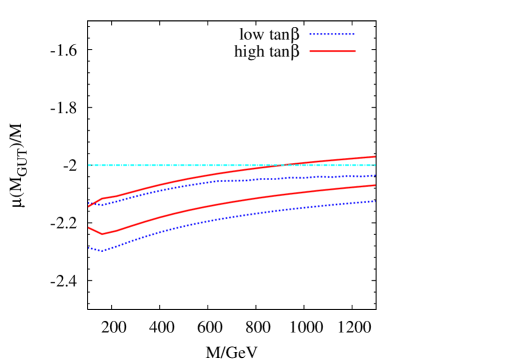
Figure 7: The ratio $\mu(M_{GUT})/M$ as required by EWSB, for the high and low $\tan\beta$ branches. In each case, the band is obtained by varying $m_{t}$ in its $2\sigma$ range. The horizontal line corresponds to $\mu(M_{GUT})/M=-2$.

In particular, we can see that a hypothetical relation $\mu(M_{GUT})=-2M$ is consistent with EWSB in the high $\tan\beta$ branch. It is also interesting that this happens for large $M$ only ($M>900$ GeV), which is compatible with the experimental constraints discussed above. So, if such a relationship was found to hold due to some underlying physics at the unification scale, one would have a model in which a little hierarchy $M_{Z}/M\sim 0.1$ could emerge without requiring a special fine-tuning among mass parameters. In such a model, in other words, the simple relationships among MSSM mass parameters at the unification scale, combined with the RG evolution of such parameters, would lead to cancellations in the low-energy Higgs potential, so that the smallness of $M_{Z}/M$ could be (at least in part) justified.

3.3 $\mu>0$ Case

We turn now to the $\mu>0$ set of solutions. Since we have found no solutions for the strict model prediction of $r_{B}=1$, we are forced to consider perturbations of the fluxed boundary conditions. Fig. 1a demonstrates that higher $m_{t}$ leads to values of $r_{B}$ closer to one, and that values of $r_{B}=0.85$ are attainable if $m_{t}=186$ GeV. We have taken these two values in order to study the scenario, but for purposes of brevity neglect to include the plots in this paper, choosing to summarise the results in text for $M=100-900$ GeV. $\tan\beta$ is in the range 26-36, monotonically increasing with $M$. The LEP2 bound on $m_{h}$ implies a mild constraint only ($M>150$ GeV). The $b\rightarrow s\gamma$ bound implies a stronger constraint ($M>500$ GeV), due to the high value for $\tan\beta$. This bound, however, is weaker than the bound that holds for $\mu<0$, because for $\mu>0$ some cancellations take place in the $b\rightarrow s\gamma$ amplitude. The advantage of $\mu>0$ is even more evident in the case of $\delta a_{\mu}$, which is positive, so that the predicted $a_{\mu}$ more easily agrees with the measured value. In fact, the constraint from $\delta a_{\mu}$ is not very restrictive ($M>230$ GeV), despite the high values for $\tan\beta$.

The model’s spectrum looks remarkably similar to Fig. 6. The main differences are that the heavy Higgs bosons have larger masses, and the lightest stau is closer in mass to the neutralino. The latter feature results in two small regions in $M$ where dark matter is compatible with the WMAP constraint. For the specified inputs, such regions have $M=160-190$ GeV and $M=640-650$ GeV. Between these two regions, $\Omega h^{2}$ is higher than the WMAP constraint, otherwise it is lower.

4 Stability of Results

We will now examine how stable the phenomenology is with respect to variations in experimental inputs, perturbations of the fluxed boundary conditions and theoretical uncertainties in the mass spectrum prediction. We will consider both $\tan\beta$ branches of the $\mu<0$ case. In particular, an important question about the high $\tan\beta$ branch is whether it is possible to obtain a solution to all the constraints with a lighter spectrum than $M\approx 1100$ GeV, taking into account various relevant uncertainties.

In order to investigate the stability of our predictions, we will vary one input or boundary condition at a time, keeping all others at their defaults. These variations will be:

• 2 $\sigma$ variations in the input value of $m_{t}$, i.e. 170 GeV $<m_{t}<$ 186 GeV.

• 2 $\sigma$ variations in the input value of $\alpha_{s}(M_{Z})$, i.e. $0.115<\alpha_{s}(M_{Z})<0.123$.

• Variations of $M_{SUSY}$ by a factor of two in each direction (setting the minimum value to be not smaller than $M_{Z}$), which should give an estimate of higher-order theoretical uncertainties (see e.g. ref. [30]).

• 10% variations in the boundary condition for $M_{1/2}$ ($0.9<M_{1/2}/M<1.1$), without changing the boundary conditions for $m_{0},A_{0},B$.

• 10% variations in the boundary condition for $B$ (that is, $0.9<r_{B}<1.1$ in eq. (3)), without changing the boundary conditions for $M_{1/2},m_{0},A_{0}$.

In practice, for a given value of $M$, we scan over 20 values of the parameter being varied, then plot the maximum and minimum values for the constraints obtained with that scan. Fig. 8 shows the effect of the above variations on some of the predictions in the high $\tan\beta$ branch (a,b,c) and in the low $\tan\beta$ branch (d). In each panel, we only show variations that have non-negligible effects.

Figure 8: Uncertainties in predictions along the $\mu<0$ high $\tan\beta$ branch in (a) the dark matter relic density $\Omega h^{2}$, (b) $BR(b\rightarrow s\gamma)$ (c) $m_{h}$. Panel (d) shows $m_{h}$ in the $\mu<0$ low $\tan\beta$ branch. In (a), the region between the two horizontal lines is favoured by the 3$\sigma$ WMAP constraint for a stable neutralino LSP making up all of the dark matter in the universe.

We first consider the high $\tan\beta$ branch. Fig. 8a shows uncertainties in the relic density prediction. The uncertainty under variations of $M_{SUSY}$ is small. Changing either the $M_{1/2}$ boundary condition by $\pm 10\%$ or the input value of $\alpha_{s}(M_{Z})$ makes a larger difference, but does not qualitatively change the region compatible with WMAP, shown by the region between the horizontal lines. However, we see that varying either $m_{t}$ or the high-scale boundary condition on $B$ makes any value $200<M<1200$ GeV compatible with the WMAP constraint. As explained previously, above $M>200$ GeV, low values of $\Omega h^{2}$ are caused when two $\chi_{1}^{0}$s annihilate via almost-resonant $s$ channel pseudo-scalar $A$ Higgs bosons, i.e. for $m_{A}\simeq 2M_{\chi_{1}^{0}}$. Since $m_{A}$ is very sensitive to variations in $m_{t}$ or in the $B$ boundary condition, the value of $M$ at which the condition $m_{A}\simeq 2M_{\chi_{1}^{0}}$ is satisfied can shift very much under such variations. Hence the constraint on $M$ from the relic density is not so stringent. However, Fig. 8b shows that $b\rightarrow s\gamma$ requires $M$ to be anyhow larger than about 1 TeV, even if we allow for variations in $m_{t}$ or in the $B$ boundary condition. Thus, it appears that we are stuck with a heavy spectrum (and the associated large fine-tuning and difficulties for detection in colliders) for the $\mu<0$ high $\tan\beta$ branch. For completeness, we also show the behaviour of $m_{h}$ in Fig. 8c, including variations. The constraint on $M$ remains quite weak, but the absolute prediction on $m_{h}$ has a strong dependence on $m_{t}$, as usual.

We turn now to the discussion of the low $\tan\beta$ branch. For default parameters, this branch is not compatible with the stable neutralino LSP assumption since the relic density predicted is much higher than the WMAP constraint, as shown previously in Fig. 3. Contrary to the case in the high $\tan\beta$ branch, this situation does not change with any variations, because none of them brings the model appreciably closer to a (co-)annihilation region. If we assume that this problem can be solved by some means (for instance by assuming that the lightest neutralino is not stable on cosmological time scales), the strongest bound on $M$ in the default calculation ($M>550$ GeV) comes from the LEP2 Higgs mass constraint, see Fig. 3b. Fig. 8d shows the behaviour of $m_{h}$ under variations. We notice that $m_{h}$ has the usual strong dependence on $m_{t}$, as well as a significant dependence on the $B$ boundary condition. Indeed, changing the latter parameter produces a significant relative change in $\tan\beta$, which in turn affects the tree-level Higgs mass (in this low $\tan\beta$ branch). Fig. 8d shows that varying either $m_{t}$ or the $B$ boundary condition results in a lower bound $M>300$ GeV. The variations induced by changes in $M_{SUSY}$ or $M_{1/2}$ have smaller effects upon the bound. The bounds coming from the anomalous magnetic moment of the muon and from $b\rightarrow s\gamma$ do show smaller variations: the bounds on $M$ can vary up to $\sim\pm 10\%$.

5 Conclusions

We have considered the phenomenology of a set of SUSY-breaking MSSM boundary conditions motivated by flux-induced SUSY breaking in Type IIB orientifold models. These boundary conditions may be interpreted as the Type IIB version of modulus-dominance SUSY-breaking considered in the past for heterotic models. The model is extremely constrained and, after imposing radiative EWSB, depends on a single parameter, the overall SUSY-breaking scale $M$. This is to be contrasted with other string inspired schemes like heterotic dilaton domination in which, even after imposing EWSB conditions, there are still two free parameters. We find it remarkable that consistent EWSB may be attained at all for our very restricted set of soft terms.

We have shown that electroweak symmetry breaking is only compatible with one sign of $\mu<0$, for which there are two solutions: one with low $\tan\beta\sim 3-5$ and one with high $\tan\beta\sim 25-40$:

• The low $\tan\beta$ solution is consistent with having a SUSY breaking parameter $M>300$ GeV depending on the precise value of $m_{t}$. This may allow for a relatively light SUSY spectrum. On the other hand this low $\tan\beta$ solution is not compatible with the lightest neutralino constituting the dark matter of the universe, since the predicted relic density is higher than that implied by WMAP and standard cosmology. Thus one would need to have an unstable neutralino, which could be due to the existence of an extra lighter SUSY particle or to the existence of R-parity violating couplings. In the latter case the collider phenomenology would very much depend on the neutralino lifetime. If it is much longer than $\mathcal{O}(10^{-6})$s the lightest neutralino will leave detectors intact; collider signatures will therefore mimic the usual missing energy R-parity conserving MSSM signatures and LHC discovery and measurements [35] should be easily possible. If the lifetime of the neutralino is shorter than $10^{-6}$s then the associated collider phenomenology will depend largely on its decay products.

• The high $\tan\beta$ branch of solutions can pass all constraints as well as provide the dark matter density compatible with WMAP constraints. The spectrum compatible with these constraints is heavy: with the LSP ($\chi_{1}^{0}$) at around 500 GeV and all sparticles other than $\chi_{2}^{0},\chi_{1}^{+}$ and ${\tilde{\tau}}_{1}$ heavier than 1 TeV. This would make sparticle measurements at the LHC practically impossible. With 100 fb^-1 integrated luminosity, SUSY should still be detectable at the LHC through the inclusive $E_{T}^{\mbox{miss}}$ measurement [36], but more luminosity would be required for other channels involving leptons.

  Due to the heavy spectrum in this high $\tan\beta$ case a certain amount of fine-tuning of the EWSB conditions would seem to be required. On the other hand we have argued that if the underlying theory predicted an approximate relationship $\mu=-2M$ at the unification scale, such fine-tuning would be substantially alleviated or even removed.