Color Superconductivity via Supersymmetry111Talk presented by N.M. at YITP workshop on Fundamental Problems and Applications of Quantum Field Theory, December 16-18, 2004, Yukawa Institute for Theoretical Physics, Kyoto, Japan and at 2004 International Workshop on Dynamical Symmetry Breaking, December 21-22, 2004, Nagoya University, Nagoya, Japan.

Nobuhito Maru222e-mail: maru@riken.jp, and Motoi Tachibana333e-mail: motoi@riken.jp

Theoretical Physics Laboratory, RIKEN

2-1 Hirosawa, Wako, Saitama, 351-0198, JAPAN

Abstract

In this talk, a supersymmetric (SUSY) composite model of color superconductivity is discussed. In this model, quark and diquark supermultiplets are dynamically generated as massless composites by a newly introduced confining gauge dynamics. It is analytically shown that the scalar component of diquark supermultiplets develops vacuum expectation value (VEV) at a certain critical chemical potential. We believe that our model well captures aspects of the diquark condensate behavior and helps our understanding of its dynamics in real QCD. The results obtained here might be useful when we consider a theory composed of quarks and diquarks.

1 Introduction

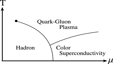
There has been much attention to color superconductivity conjectured to appear in QCD at high baryon density [1]. Conjectured phase diagram is shown in Fig 1. Previous studies of QCD with this direction were limited to very high density where the theory is perturbative because of the asymptotic freedom [2]. But our interest is the low energy physics where the theory is strongly coupled. Therefore, it would be interesting to find QCD-like theories calculable even at lower density, namely in the strong coupling regime. In this viewpoint, Nambu-Jona-Lasino model has been well studied by many people [3].

Recently, another approach using a SUSY gauge theory was proposed [4], where the breaking pattern of global symmetries in a softly broken SUSY QCD at finite chemical potential was investigated and compared to that obtained from the analysis via nonsupersymmetric QCD [5]. In particular, the phase structure associated with baryon number symmetry $U(1)_{B}$ was extensively studied. However, the color variant quantity such as diquark responsible for color superconductivity was not included in the low energy effective theory. Therefore, we should somehow extend their analysis to have diquark degrees of freedom. In the light of this fact, we propose here a SUSY model of color superconductivity where quarks and diquarks are dynamically generated as composites by a newly introduced strong gauge dynamics [6].

Refer to caption
Figure 1: (Conjectured) phase diagram of hot and dense quark matter.

2 Model

Our model is based on an ${\cal N}=1$ SUSY $SO(N_{c})$ gauge theory with $N_{f}(=N_{c}-4)$ flavors [7]. The flavor symmetry in the original model $SU(N_{f})$ is extended to $SU(3)_{C}\times SU(N_{f})_{L}\times SU(N_{f})_{R}$, where $SU(3)_{C}$ is a usual color gauge group and is assumed to be weakly gauged compared to $SO(N_{c}=6N_{f}+5)$ gauge group, $SU(N_{f})_{L}\times SU(N_{f})_{R}$ is a chiral symmetry. Matter content of the supermultiplets is summarized below;

$\displaystyle Q$ $\displaystyle=$ (ย ย ย ,ย ย ย ,ย ย ย ,๐Ÿ)1,1,1,subscriptย ย ย ย ย ย ย ย ย 1111\displaystyle(\>{\vbox{\vbox{\hrule height=0.6pt\hbox{\vrule width=0.6pt,height=5.0pt\kern 5.0pt\vrule width=0.6pt,height=5.0pt} \hrule height=0.6pt} }}\>\>,\>{\vbox{\vbox{\hrule height=0.6pt\hbox{\vrule width=0.6pt,height=5.0pt\kern 5.0pt\vrule width=0.6pt,height=5.0pt} \hrule height=0.6pt} }}\>\>,\>{\vbox{\vbox{\hrule height=0.6pt\hbox{\vrule width=0.6pt,height=5.0pt\kern 5.0pt\vrule width=0.6pt,height=5.0pt} \hrule height=0.6pt} }}\>\>,{\bf 1})_{1,1,1}, (1)
$\displaystyle\bar{Q}$ $\displaystyle=$ (ย ย ย ,ย ย ย ยฏ,๐Ÿ,ย ย ย ยฏ)โˆ’1,1,1,subscriptย ย ย ยฏย ย ย 1ยฏย ย ย 111\displaystyle(\>{\vbox{\vbox{\hrule height=0.6pt\hbox{\vrule width=0.6pt,height=5.0pt\kern 5.0pt\vrule width=0.6pt,height=5.0pt} \hrule height=0.6pt} }}\>\>,\>\overline{{\vbox{\vbox{\hrule height=0.6pt\hbox{\vrule width=0.6pt,height=5.0pt\kern 5.0pt\vrule width=0.6pt,height=5.0pt} \hrule height=0.6pt} }}}\>\>,{\bf 1},\>\overline{{\vbox{\vbox{\hrule height=0.6pt\hbox{\vrule width=0.6pt,height=5.0pt\kern 5.0pt\vrule width=0.6pt,height=5.0pt} \hrule height=0.6pt} }}}\>\>)_{-1,1,1}, (2)
$\displaystyle X$ $\displaystyle=$ (ย ย ย ,๐Ÿ,๐Ÿ,๐Ÿ)0,โˆ’6โ€‹Nf,3โˆ’Nsubscriptย ย ย 11106subscript๐‘๐‘“3๐‘\displaystyle(\>{\vbox{\vbox{\hrule height=0.6pt\hbox{\vrule width=0.6pt,height=5.0pt\kern 5.0pt\vrule width=0.6pt,height=5.0pt} \hrule height=0.6pt} }}\>\>,{\bf 1},{\bf 1},{\bf 1})_{0,-6N_{f},3-N} (3)

where the representations in the parenthesis are transformation properties under the group $SO(6N_{f}+5)\times SU(3)_{C}\times SU(N_{f})_{L}\times SU(N_{f})_{R}$. The numbers in the subscripts are charges for nonanomalous $U(1)$ global symmetries $U(1)_{B}\times U(1)_{A}\times U(1)_{R}$, which each $U(1)$ symmetry is linear combination of the original anomalous $U(1)$ symmetries.

$SO$ gauge theory mentioned above is known to be in the cofining phase [7]. Massless degrees of freedom describing the low energy effective theory below the dynamical scale $\Lambda_{SO}$ are given by the following gauge invariant composite superfields:

$\displaystyle(Q^{2})$ $\displaystyle=$ (ย ย ย ยฏ,ย ย ย ย ย ,๐Ÿ)2,2,2,(ย ย ย ,ย ย ย ,๐Ÿ)2,2,2,subscriptยฏย ย ย ย ย ย ย ย 1222subscriptย ย ย ย ย ย 1222\displaystyle(\>\overline{{\vbox{\vbox{\hrule height=0.6pt\hbox{\vrule width=0.6pt,height=5.0pt\kern 5.0pt\vrule width=0.6pt,height=5.0pt} \hrule height=0.6pt} }}}\>\>,\>{\vbox{\vbox{\hrule height=0.6pt\hbox{\vrule width=0.6pt,height=5.0pt\kern 5.0pt\vrule width=0.6pt,height=5.0pt} \hrule height=0.6pt\hbox{\vrule width=0.6pt,height=5.0pt\kern 5.0pt\vrule width=0.6pt,height=5.0pt} \hrule height=0.6pt} }}\>\>,{\bf 1})_{2,2,2},(\>{\vbox{\vbox{\hrule height=0.6pt\hbox{\vrule width=0.6pt,height=5.0pt\kern 5.0pt\vrule width=0.6pt,height=5.0pt\kern 5.0pt\vrule width=0.6pt,height=5.0pt} \hrule height=0.6pt} }}\>\>,\>{\vbox{\vbox{\hrule height=0.6pt\hbox{\vrule width=0.6pt,height=5.0pt\kern 5.0pt\vrule width=0.6pt,height=5.0pt\kern 5.0pt\vrule width=0.6pt,height=5.0pt} \hrule height=0.6pt} }}\>\>,{\bf 1})_{2,2,2}, (4)
$\displaystyle(\bar{Q}^{2})$ $\displaystyle=$ (ย ย ย ,๐Ÿ,ย ย ย ย ย ยฏ)โˆ’2,2,2,(ย ย ย ยฏ,๐Ÿ,ย ย ย ยฏ)โˆ’2,2,2,subscriptย ย ย 1ยฏย ย ย ย ย 222subscriptยฏย ย ย 1ยฏย ย ย 222\displaystyle(\>{\vbox{\vbox{\hrule height=0.6pt\hbox{\vrule width=0.6pt,height=5.0pt\kern 5.0pt\vrule width=0.6pt,height=5.0pt} \hrule height=0.6pt} }}\>\>,{\bf 1},\overline{\>{\vbox{\vbox{\hrule height=0.6pt\hbox{\vrule width=0.6pt,height=5.0pt\kern 5.0pt\vrule width=0.6pt,height=5.0pt} \hrule height=0.6pt\hbox{\vrule width=0.6pt,height=5.0pt\kern 5.0pt\vrule width=0.6pt,height=5.0pt} \hrule height=0.6pt} }}\>\>})_{-2,2,2},(\overline{\>{\vbox{\vbox{\hrule height=0.6pt\hbox{\vrule width=0.6pt,height=5.0pt\kern 5.0pt\vrule width=0.6pt,height=5.0pt\kern 5.0pt\vrule width=0.6pt,height=5.0pt} \hrule height=0.6pt} }}\>\>},{\bf 1},\overline{\>{\vbox{\vbox{\hrule height=0.6pt\hbox{\vrule width=0.6pt,height=5.0pt\kern 5.0pt\vrule width=0.6pt,height=5.0pt\kern 5.0pt\vrule width=0.6pt,height=5.0pt} \hrule height=0.6pt} }}\>\>})_{-2,2,2}, (5)
$\displaystyle(X^{2})$ $\displaystyle=$ $\displaystyle({\bf 1},{\bf 1},{\bf 1})_{0,-12N_{f},6-2N},$ (6)
$\displaystyle(QX)$ $\displaystyle=$ (ย ย ย ,ย ย ย ,๐Ÿ)1,1โˆ’6โ€‹Nf,4โˆ’N,subscriptย ย ย ย ย ย 1116subscript๐‘๐‘“4๐‘\displaystyle(\>{\vbox{\vbox{\hrule height=0.6pt\hbox{\vrule width=0.6pt,height=5.0pt\kern 5.0pt\vrule width=0.6pt,height=5.0pt} \hrule height=0.6pt} }}\>\>,\>{\vbox{\vbox{\hrule height=0.6pt\hbox{\vrule width=0.6pt,height=5.0pt\kern 5.0pt\vrule width=0.6pt,height=5.0pt} \hrule height=0.6pt} }}\>\>,{\bf 1})_{1,1-6N_{f},4-N}, (7)
$\displaystyle(\bar{Q}X)$ $\displaystyle=$ (ย ย ย ยฏ,๐Ÿ,ย ย ย ยฏ)โˆ’1,1โˆ’6โ€‹Nf,4โˆ’N,subscriptยฏย ย ย 1ยฏย ย ย 116subscript๐‘๐‘“4๐‘\displaystyle(\>\overline{{\vbox{\vbox{\hrule height=0.6pt\hbox{\vrule width=0.6pt,height=5.0pt\kern 5.0pt\vrule width=0.6pt,height=5.0pt} \hrule height=0.6pt} }}}\>\>,{\bf 1},\>\overline{{\vbox{\vbox{\hrule height=0.6pt\hbox{\vrule width=0.6pt,height=5.0pt\kern 5.0pt\vrule width=0.6pt,height=5.0pt} \hrule height=0.6pt} }}}\>\>)_{-1,1-6N_{f},4-N}, (8)
$\displaystyle(Q\bar{Q})$ $\displaystyle=$ (๐Ÿ,ย ย ย ,ย ย ย ยฏ)0,2,2,(๐Ÿ–,ย ย ย ,ย ย ย ยฏ)0,2,2subscript1ย ย ย ยฏย ย ย 022subscript8ย ย ย ยฏย ย ย 022\displaystyle({\bf 1},\>{\vbox{\vbox{\hrule height=0.6pt\hbox{\vrule width=0.6pt,height=5.0pt\kern 5.0pt\vrule width=0.6pt,height=5.0pt} \hrule height=0.6pt} }}\>\>,\>\overline{{\vbox{\vbox{\hrule height=0.6pt\hbox{\vrule width=0.6pt,height=5.0pt\kern 5.0pt\vrule width=0.6pt,height=5.0pt} \hrule height=0.6pt} }}}\>\>)_{0,2,2},({\bf 8},\>{\vbox{\vbox{\hrule height=0.6pt\hbox{\vrule width=0.6pt,height=5.0pt\kern 5.0pt\vrule width=0.6pt,height=5.0pt} \hrule height=0.6pt} }}\>\>,\>\overline{{\vbox{\vbox{\hrule height=0.6pt\hbox{\vrule width=0.6pt,height=5.0pt\kern 5.0pt\vrule width=0.6pt,height=5.0pt} \hrule height=0.6pt} }}}\>\>)_{0,2,2} (9)

where the representations in the parenthesis are those under the group $SU(3)_{C}\times SU(N_{f})_{L}\times SU(N_{f})_{R}$. The numbers in the subscripts are charges for nonanomalous $U(1)$ symmetries $U(1)_{B}\times U(1)_{A}\times U(1)_{R}$. Note that $Q^{2}(\bar{Q}^{2})$ has symmetric (its conjugate) and anti-symmetric (its conjugate) representations under $SU(3)_{C}\times SU(N_{f})_{L}\times SU(N_{f})_{R}$ because $SO(N)$ indices are contracted symmetrically and the superfields are bosonic. One can see from the transformation properties that superfields with anti-symmetric representation in $Q^{2}$ and $\bar{Q}^{2}$ correspond to โ€œdiquarkโ€ supermultiplet and $QX$ and $\bar{Q}X$ correspond to โ€œquarkโ€ supermultiplet. Thus, quark and diquark supermultiplets are generated as composites and coexist in the low energy theory. What is more nontrivial is that these composites satisfy tโ€™ Hooft anomaly matching conditions, which implies that massless degrees of freedom are completely determined despite the strong coupling in the infrared below the scale $\Lambda_{SO}$.

Incorpolating the chemical potential can be regarded as the time component of a fictitious gauge field of $U(1)_{B}$ symmetry at zero temperature. For fermion field, it is described as

โ„’ฯˆ=iฯˆยฏโˆ‚/ฯˆ,ฮ”โ„’=ฮผฯˆโ€ ฯˆ=ฮผฯˆยฏฮณ0ฯˆโ‡’โ„’ฯˆ+ฮ”โ„’=iฯˆยฏ(โˆ‚/โˆ’igA/)ฯˆ,\displaystyle{\cal L}_{\psi}=i\bar{\psi}\partial\!\!\!/\psi,\quad\Delta{\cal L}=\mu\psi^{\dagger}\psi=\mu\bar{\psi}\gamma^{0}\psi\Rightarrow{\cal L}_{\psi}+\Delta{\cal L}=i\bar{\psi}(\partial\!\!\!/-igA\!\!\!/)\psi, (10)

where $A_{\nu}={\rm diag}(\mu/g,0,0,0)$, $g$ is the gauge coupling constant of $U(1)_{B}$. Since we are considering a SUSY theory, the corresponding argument for scalar fields is present,

โ„’ฯ•+ฮ”โ€‹โ„’=(โˆ‚ฮฝโˆ’iโ€‹gโ€‹Aฮฝ)โ€ โ€‹ฯ•โ€ โ€‹(โˆ‚ฮฝโˆ’iโ€‹gโ€‹Aฮฝ)โ€‹ฯ•.subscriptโ„’italic-ฯ•ฮ”โ„’superscriptsuperscript๐œˆ๐‘–๐‘”superscript๐ด๐œˆโ€ superscriptitalic-ฯ•โ€ subscript๐œˆ๐‘–๐‘”subscript๐ด๐œˆitalic-ฯ•\displaystyle{\cal L}_{\phi}+\Delta{\cal L}=(\partial^{\nu}-igA^{\nu})^{\dagger}\phi^{\dagger}(\partial_{\nu}-igA_{\nu})\phi. (11)

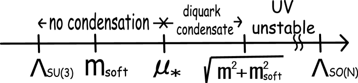
We notice that the above scalar Lagrangian with the finite chemical potential includes a SUSY breaking scalar mass term +ฮผ2โ€‹ฯ•โ€ โ€‹ฯ•superscript๐œ‡2superscriptitalic-ฯ•โ€ italic-ฯ•+\mu^{2}\phi^{\dagger}\phi. Therefore, we impose the condition $\mu<\Lambda_{SO}$ since we can utilize exact results in SUSY gauge theory reliably. Furthermore, the SUSY breaking scalar mass squared is found to be negative, namely tachyon, which implies that UV theory is unstable. In order to avoid this situation, we have to add both (positive) SUSY breaking mass in the potential and SUSY mass in the superpotential.444The same symbols for the superfields and the corresponding scalar components are used.

$\displaystyle\Delta W_{{\rm SUSY}}$ $\displaystyle=$ $\displaystyle m_{ij}\bar{Q}_{i}Q_{j}\Rightarrow\Delta V_{{\rm SUSY}}=m^{2}(|Q|^{2}+|\bar{Q}|^{2}),$ (12)
$\displaystyle\Delta V_{{\rm SUSY~{}breaking}}$ $\displaystyle=$ $\displaystyle m^{2}_{{\rm soft}}(|Q|^{2}+|\bar{Q}|^{2}),$ (13)

which results in the following UV potential

$\displaystyle V_{{\rm UV}}$ $\displaystyle=$ $\displaystyle(m^{2}+m^{2}_{{\rm soft}}-\mu^{2})(|Q|^{2}+|\bar{Q}|^{2}).$ (14)

As will be shown later, the critical chemical potential where the color superconductivity happens is larger than the soft SUSY breaking mass. Thus, we need to add SUSY masses in the superpotential and have to impose the condition $m^{2}+m^{2}_{{\rm soft}}-\mu^{2}>0$ to obtain the UV stable potential.

The low energy superpotential is generated by the gaugino condensation in the unbroken gauge group $SO(4)\simeq SU(2)_{L}\times SU(2)_{R}$,

$\displaystyle W_{{\rm eff}}=2(\epsilon_{L}+\epsilon_{R})\left(\frac{\Lambda_{SO(N)}^{6N_{f}+4}}{[{\rm det}(Q\bar{Q})]X}\right)$ (15)

where $\epsilon_{L,R}=\pm 1$ are phase factors reflecting the number of SUSY vacua suggested from Witten index [8]. There are two physically inequivalent branches, one is $W_{{\rm eff}}=0(\epsilon_{L}=-\epsilon_{R})$ and the other is Weffโ‰ 0โ€‹(ฯตL=ฯตR)subscript๐‘Šeff0subscriptitalic-ฯต๐ฟsubscriptitalic-ฯต๐‘…W_{{\rm eff}}\neq 0(\epsilon_{L}=\epsilon_{R}). Here, we focus on the former case throughout this article, which is relevant for the color supercoductivity.

In order to obtain the scalar potential, we need Kรคhler potential for composite fields. It is impossible to determine the Kรคhler potential exactly because of its nonholomorphicity, but the leading term can be fixed by using the argument of analytic continuation into superspace [9] in the expansion of the SUSY breaking scale to $\Lambda_{SO}$. The effective Kรคhler potential for composite fields is fixed by symmetries and the renormalization group (RG) invariance,

$\displaystyle K_{{\rm eff}}$ $\displaystyle=$ c(Q2)โ€‹๐’ต(Q2)Iโ€‹(Q2)โ€ โ€‹e2โ€‹VBโ€‹(Q2)+c(Qยฏ2)โ€‹๐’ต(Qยฏ2)Iโ€‹(Qยฏ2)โ€ โ€‹eโˆ’2โ€‹VBโ€‹(Qยฏ2)subscript๐‘superscript๐‘„2subscript๐’ตsuperscript๐‘„2๐ผsuperscriptsuperscript๐‘„2โ€ superscript๐‘’2subscript๐‘‰๐ตsuperscript๐‘„2subscript๐‘superscriptยฏ๐‘„2subscript๐’ตsuperscriptยฏ๐‘„2๐ผsuperscriptsuperscriptยฏ๐‘„2โ€ superscript๐‘’2subscript๐‘‰๐ตsuperscriptยฏ๐‘„2\displaystyle c_{(Q^{2})}\frac{{\cal Z}_{(Q^{2})}}{I}(Q^{2})^{\dagger}e^{2V_{B}}(Q^{2})+c_{(\bar{Q}^{2})}\frac{{\cal Z}_{(\bar{Q}^{2})}}{I}(\bar{Q}^{2})^{\dagger}e^{-2V_{B}}(\bar{Q}^{2}) (16)
$\displaystyle+$ c(X2)โ€‹๐’ต(X2)Iโ€‹(X2)โ€ โ€‹(X2)+c(Qโ€‹X)โ€‹๐’ต(Qโ€‹X)Iโ€‹(Qโ€‹X)โ€ โ€‹eVBโ€‹(Qโ€‹X)subscript๐‘superscript๐‘‹2subscript๐’ตsuperscript๐‘‹2๐ผsuperscriptsuperscript๐‘‹2โ€ superscript๐‘‹2subscript๐‘๐‘„๐‘‹subscript๐’ต๐‘„๐‘‹๐ผsuperscript๐‘„๐‘‹โ€ superscript๐‘’subscript๐‘‰๐ต๐‘„๐‘‹\displaystyle c_{(X^{2})}\frac{{\cal Z}_{(X^{2})}}{I}(X^{2})^{\dagger}(X^{2})+c_{(QX)}\frac{{\cal Z}_{(QX)}}{I}(QX)^{\dagger}e^{V_{B}}(QX)
$\displaystyle+$ c(Qยฏโ€‹X)โ€‹๐’ต(Qยฏโ€‹X)Iโ€‹(Qยฏโ€‹X)โ€ โ€‹eโˆ’VBโ€‹(Qยฏโ€‹X)+c(Qโ€‹Qยฏ)โ€‹๐’ต(Qโ€‹Qยฏ)Iโ€‹(Qโ€‹Qยฏ)โ€ โ€‹(Qโ€‹Qยฏ),subscript๐‘ยฏ๐‘„๐‘‹subscript๐’ตยฏ๐‘„๐‘‹๐ผsuperscriptยฏ๐‘„๐‘‹โ€ superscript๐‘’subscript๐‘‰๐ตยฏ๐‘„๐‘‹subscript๐‘๐‘„ยฏ๐‘„subscript๐’ต๐‘„ยฏ๐‘„๐ผsuperscript๐‘„ยฏ๐‘„โ€ ๐‘„ยฏ๐‘„\displaystyle c_{(\bar{Q}X)}\frac{{\cal Z}_{(\bar{Q}X)}}{I}(\bar{Q}X)^{\dagger}e^{-V_{B}}(\bar{Q}X)+c_{(Q\bar{Q})}\frac{{\cal Z}_{(Q\bar{Q})}}{I}(Q\bar{Q})^{\dagger}(Q\bar{Q}),

where overall coefficients $c$โ€™s are of order ${\cal O}(1)$ unknown constants. The exponential factors for QCD are suppressed. $V_{B}$ is a background vector superfield $U(1)_{B}$ with a VEV $\langle V_{B}\rangle=\bar{\theta}\sigma^{\mu}\theta\langle A_{\mu}\rangle,\quad\langle A_{\mu}\rangle=(\mu/g_{B},0,0,0)$. $g_{B}$ is a gauge coupling constant and $\mu$ is a chemical potential. Wave function renomalization constants $Z_{i}$ are promoted to a superfield ${\cal Z}_{i}$

$${\cal Z}_{i}=Z_{i}\left[1-\theta^{2}\bar{\theta}^{2}m_{{\rm soft}}^{2}\right]$$ (17)

where $m_{{\rm soft}}$ is a soft SUSY breaking scalar mass in the UV and taken to be universal. The quantity $I$ is a spurious $U(1)$ symmetry and the RG invariant superfield,

I=ฮ›hโ€ โ€‹๐’ต2โ€‹T/b0โ€‹ฮ›h๐ผsuperscriptsubscriptฮ›โ„Žโ€ superscript๐’ต2๐‘‡subscript๐‘0subscriptฮ›โ„ŽI=\Lambda_{h}^{\dagger}{\cal Z}^{2T/b_{0}}\Lambda_{h} (18)

where $T$ is the total Dynkin index of the matter fields, $b_{0}$ is the 1-loop beta function coefficient and $\Lambda_{h}=\mu_{UV}{\rm exp}[-8\pi^{2}S(\mu_{UV})/b_{0}],S(\mu_{UV})=\frac{1}{g^{2}}\left(1+\theta^{2}\frac{m_{\lambda}}{2}\right)(m_{\lambda}:{\rm gaugino~{}mass})$. Note that a spurious $U(1)$ transformations are given by

Qrโ†’eAโ€‹Qr,๐’ตrโ†’eA+Aโ€ โ€‹๐’ตr,formulae-sequenceโ†’subscript๐‘„๐‘Ÿsuperscript๐‘’๐ดsubscript๐‘„๐‘Ÿโ†’subscript๐’ต๐‘Ÿsuperscript๐‘’๐ดsuperscript๐ดโ€ subscript๐’ต๐‘Ÿ\displaystyle Q_{r}\to e^{A}Q_{r},{\cal Z}_{r}\to e^{A+A^{\dagger}}{\cal Z}_{r}, (19)
$\displaystyle S(\mu_{{\rm UV}})\to S(\mu_{{\rm UV}})-\frac{T}{4\pi^{2}}A$ (20)

where $A$ is a chiral superfield.

Now, we are ready to obtain scalar masses for composites from the above Kรคhler potential,

$\displaystyle\tilde{m}^{2}_{(Q^{2})}=\tilde{m}^{2}_{(\bar{Q}^{2})}$ $\displaystyle=$ $\displaystyle\frac{6N_{f}+7}{2(3N_{f}+2)}m_{{\rm soft}}^{2}-\mu^{2},$ (21)
$\displaystyle\tilde{m}^{2}_{(X^{2})}=\tilde{m}^{2}_{(Q\bar{Q})}$ $\displaystyle=$ $\displaystyle\frac{6N_{f}+7}{2(3N_{f}+2)}m^{2}_{{\rm soft}}>0,$ (22)
$\displaystyle\tilde{m}^{2}_{(QX)}=\tilde{m}^{2}_{(\bar{Q}X)}$ $\displaystyle=$ $\displaystyle\frac{6N_{f}+7}{2(3N_{f}+2)}m_{{\rm soft}}^{2}-\frac{1}{4}\mu^{2}.$ (23)

One can see that $\tilde{m}^{2}_{(Q^{2})}=\tilde{m}^{2}_{(\bar{Q}^{2})}<0$ if the chemical potential is larger than some critical value $\mu>\mu_{*}\equiv\sqrt{\frac{6N_{f}+7}{2(3N_{f}+2)}}m_{{\rm soft}}$. Thus, the diquarks condensate at the finite chemical potential, but the condensate is the scalar component of the diquark supermultiplet.

The above argument for the behavior of the scalar component of the diquark supermultiplet is valid for the vanishing superpotential case. For the case with nonvanishing superpotetial, on the other hand, it is found that the scalar potential is very complicated,

$\displaystyle V$ $\displaystyle=$ $\displaystyle\left(\frac{\partial^{2}K_{{\rm eff}}}{\partial\Phi_{i}\partial\Phi^{*}_{j}}\right)^{-1}\left(\frac{\partial W_{{\rm eff}}}{\partial\Phi_{i}}\right)\left(\frac{\partial W^{*}_{{\rm eff}}}{\partial\Phi^{*}_{j}}\right)\Lambda^{2}_{SO(N)}$ (24)
$\displaystyle+$ $\displaystyle\frac{1}{\Lambda^{2}_{SO(N)}}\left[\tilde{m}^{2}_{(Q^{2})}|(Q^{2})|^{2}+\tilde{m}^{2}_{(\bar{Q}^{2})}|(\bar{Q}^{2})|^{2}\right.$
$\displaystyle+$ $\displaystyle\left.\tilde{m}^{2}_{(X^{2})}|(X^{2})|^{2}+\tilde{m}^{2}_{(QX)}|(QX)|^{2}+\tilde{m}^{2}_{(\bar{Q}X)}|(\bar{Q}X)|^{2}+\tilde{m}^{2}_{(Q\bar{Q})}|(Q\bar{Q})|^{2}\right]$

where $\Phi_{i}$ denote the scalar component of composite superfields. $W_{{\rm eff}}$ includes SUSY mass terms. Therefore, we give here a qualitative discussion on the scalar potential behavior instead of an explicit minimization of the scalar potential. Note that F-term contributions to the scalar potential in the first line have a runaway behavior, which make the fields VEV away from the origin. For $\mu=0$, all SUSY breaking scalar mass squareds are positive, which set the fields VEV at the origin. Therefore all composites are expected to develop nonvanishing VEVs by balancing terms between the runaway potential and the SUSY breaking scalar mass terms. Even if we take into account that the scalar diquark mass squareds become negative for $\mu>\mu_{*}$, qualitative features of phase transition remains unchanged. In any case, the case of nonzero superpotential is irrelevant to the phase of color superconductivity of our interest. Even if we compare the vacuum energy in both cases, the case with vanishing superpotential seems to be energetically favored.

3 Summary

We have proposed a SUSY composite model of color superconductivity, which is based on a SUSY $SO(N_{f}+4)$ gauge theory with $N_{f}$ flavors. This model is in the confining phase in the infrared region and qurak and diquark supermultilets are dynamically generated as massless degrees of freedom by a newly introduced $SO$ strong gauge dynamics. Remarkably, massless degrees of freedom below the confining scale are completely determined since all independent composites satisfy anomaly matching conditions.

We have analytically shown that the scalar component of the diquark supermultiplets develop VEV at some critical chemical potential. The schematic picture of phase diagram is shown in Fig 2. Although the model is not fully realistic in that the scalar component of diquark supermultiplet (not diquarks themselves) condense, we believe that it well captures some important aspects of the diquark condensation behavior and helps our understanding for the color superconductivity in real QCD. If there is a certain intermediate region of the chemical potential where quarks are deconfined but not superconducting yet, owing to the strong quark-quark correlation, the system may be well described by a compositon of quarks and diquarks. Then the analysis performed in this paper will help us with comprehending the behavior of such a system.

As future directions, it is interesting to extend our analysis to different flavor cases. In particular, Seiberg dual description [10] might give a better understanding of color superconductivity. In order to fully understand the phase structure of QCD, it is necessary to take into account the finite temperature effects and then to study the scalar component of the diquark supermultiplet condensation behavior on the temperature-chemical potential plane as shown in Fig 1.

Refer to caption
Figure 2: Relation among various scales are displayed. Horizontal axis means the energy scale. The possible range of the chemical potential is below $\sqrt{m^{2}+m^{2}_{{\rm soft}}}$. There is no condensation when the chemical potential is between QCD scale $\Lambda_{{\rm SU(3)}}$ and the critical chemical potential $\mu_{*}$. The condensation of the scalar component of the diquark supermultiplet occurs when the chemical potential is between $\mu_{*}$ and $\sqrt{m^{2}+m^{2}_{{\rm soft}}}$. UV theory becomes unstable if the chemical potetntial is beyond the scale $\sqrt{m^{2}+m^{2}_{{\rm soft}}}$.

Acknowledgments

We would like to thank the organizers of the workshop for giving us an opportunity to present this talk. We are supported by Special Postdoctoral Researchers Program at RIKEN (No.ย A12-52040(N.M.) and No.ย A12-52010(M.T.)).

References

  • [1] D.ย Bailin and A.ย Love, Phys. Rep. 107, 325 (1984); M.ย Iwasaki and T.ย Iwado, Phys. Lett. B 350, 163 (1995); M.ย Alford, K.ย Rajagopal and F.ย Wilczek, Phys. Lett. B 422, 247 (1998) [arXiv:hep-ph/9711395]; R.ย Rapp, T.ย Schafer, E.ย V.ย Shuryak, and M.ย Velkovsky, Phys. Rev. Lett. 81, 53 (1998) [arXiv:hep-ph/9711396].
  • [2] D.ย T.ย Son, Phys. Rev. D59, 094019 (1999) [arXiv:hep-ph/9812287].
  • [3] For instance, see M.ย Kitazawa, T.ย Koide, T.ย Kunihiro and Y.ย Nemoto, Prog. Theor. Phys. 108, 929 (2002) [arXiv:hep-ph/0207255].
  • [4] R. Harnik, D. Larson and H. Murayama, โ€œSupersymmetric Color Superconductivityโ€, JHEP 0403 (2004) 049.
  • [5] T. Schafer, Nucl. Phys. B 575, 269 (2000) [arXiv:hep-ph/9909574]; T. Schafer, Phys. Rev. D62, 094007 (2000) [arXiv:hep-ph/0006034].
  • [6] N. Maru and M. Tachibana, โ€œColor Superconductivity from Supersymmetryโ€, hep-ph/0411079.
  • [7] K.A. Intriligator and N. Seiberg, โ€œDuality, monopoles, dyons, confinement and oblique confinement in supersymmetric SO(N(c)) gauge theories,โ€ Nucl. Phys. B444 (1995) 125.
  • [8] E.ย Witten, Nucl.ย Phys.ย B 202, 253 (1982).
  • [9] N.ย Arkani-Hamed and R.ย Rattazzi, Phys.ย Lett.ย B 454, 290 (1999) [arXiv:hep-th/9804068].
  • [10] N.ย Seiberg, Nucl.ย Phys.ย B 435, 129 (1995) [arXiv:hep-th/9411149].