Abstract

We carefully analyse the present experimental evidence for a complex CKM matrix, even allowing for New Physics contributions to $\epsilon_{K}$, $a_{J/\Psi K_{S}}$, $\Delta M_{B_{d}}$, $\Delta M_{B_{s}}$, and the $\Delta I=1/2$ piece of $B\to\rho\rho$ and $B\to\rho\pi$. We emphasize the crucial rôle played by the angle $\gamma$ in both providing irrefutable evidence for a complex CKM matrix and placing constraints on the size of NP contributions. It is shown that even if one allows for New Physics a real CKM matrix is excluded at a 99.92% C.L., and the probability for the phase $\gamma$ to be in the interval $[-170^{\circ};-10^{\circ}]\cup[10^{\circ};170^{\circ}]$ is 99.7%.

1 Introduction

At present, the Cabibbo–Kobayashi–Maskawa (CKM) [1] mechanism for flavour mixing and CP violation is in agreement with all available experimental data. This is a remarkable success, since it is achieved with a relatively small number of parameters. Once the experimental values of $\left|V_{us}\right|,\left|V_{cb}\right|$ and $\left|V_{ub}\right|$ are used to fix the angles $\theta_{12},\theta_{23}$ and $\theta_{13}$ of the standard parametrization, one has to fit, with a single parameter $\delta_{13}$, the experimental values of a large number of quantities, including $\epsilon_{K},\sin\left(2\beta\right),\Delta M_{B_{d}}$, as well as the bound on $\Delta M_{B_{s}}$. This impressive result is nicely represented in the usual unitarity triangle fits [2]. In view of the remarkable success of the Standard Model, it is plausible that the CKM mechanism gives the dominant contribution to mixing and CP violation at low energies, although there is still significant room for New Physics (NP).

In this paper, we address the question of how the data available at present already provide an irrefutable proof that the CKM matrix is “non-trivially complex”, thus implying that the charged weak-current interactions violate CP. Obviously, in the framework of the Standard Model (SM), the CKM matrix has to be complex, in order to account for the observed CP violation, both in the kaon and in the B sector. The above question only becomes non-trivial if one allows for the presence of NP [3]. We shall carefully analyse the present experimental indications in favour of a complex CKM matrix, correcting at the same time various misleading and in some cases erroneous statements one finds in the literature.

To have an irrefutable proof that the CKM matrix is complex is of the utmost importance in order to investigate the origin of CP violation, as well as to analyse what classes of theories of CP violation are viable in view of the present experimental data provided by B-factories. For example, one of the crucial questions concerning the origin of CP violation is whether CP is violated explicitly in the Lagrangian through the introduction of complex Yukawa couplings or, on the contrary, CP is a good symmetry of the Lagrangian, only spontaneously broken by the vacuum. There are two classes of theories with spontaneous CP violation:

1. Those where the phases arising from the vacuum lead to a complex CKM matrix, in spite of having real Yukawa couplings. In this class of theories, there are in general more than one source of CP violation, namely the usual KM mechanism, together with some new sources of CP violation.

2. Models where all phases can be removed from the CKM matrix and thus CP violation arises exclusively from New Physics.

Examples of class i) are, for instance, two Higgs doublet extensions of the SM with spontaneous CP violation, without natural flavour conservation (NFC) in the Higgs sector [4, 5], as well as models where CP is broken at a high energy scale [6] through a phase in the vacuum expectation value (vev) of a complex singlet, which in turn generates a non-trivially complex CKM matrix through the mixing of isosinglet quarks with standard quarks. Examples of class ii) are the simplest supersymmetric extensions of the SM with spontaneous CP violation [7], as well as three Higgs doublet models with spontaneous CP violation [8] and NFC in the Higgs sector.

It is clear that if it can be proved that experimental data constrain the CKM matrix to be complex, even allowing for the presence of New Physics, the only models of spontaneous CP violation that are viable belong to class i).

The paper is organized as follows. In the next section we specify what our assumptions about NP are and we address the question of how to obtain evidence for a complex CKM matrix which would not be affected by the presence of this type of NP. In section 3 we discuss the possibility of obtaining an experimental proof that the CKM matrix is complex, from the measurement of four indepedent moduli of this matrix. We argue that the cleanest proof would be obtained if one would use only moduli from the first two rows of the CKM matrix. However, we point out that contrary to some statements in the literature, this proof cannot be obtained in practice, since it would require totally unrealistic precision in the measurement of $\left|V_{us}\right|$, $\left|V_{cd}\right|$. In section 4 we analyse the impact of the measurement of $\Delta M_{B_{d}}$ and $a_{J/\Psi K_{S}}$ and introduce a convenient parametrization of NP. In section 5 we emphasize the importance of a measurement of $\gamma$ either direct or through the combined measurement of $\overline{\beta}$, $\overline{\alpha}$. Finally, we present our summary and conclusions in section 6.

2 Evidence for a complex CKM matrix unaffected by the presence of New Physics

Our assumptions about NP will be the following. We will assume that in weak processes where the SM contributes at tree level, NP contributions are negligible, while NP may be relevant to weak processes where the SM only contributes at the loop level. This is a rather mild assumption on NP. In addition, for the moment we will also assume that the 3$\times$3 CKM matrix is unitary, but we will come back to this point later. An example of this framework is the minimal supersymmetric standard model (MSSM).

This scenario implies that NP could be competing with any SM loop and more likely in $K^{0}$–$\bar{K}^{0}$, $B_{d}^{0}$–$\bar{B}_{d}^{0}$, $B_{s}^{0}$–$\bar{B}_{s}^{0}$ and $D^{0}$–$\bar{D}^{0}$ mixing. Therefore, the usual interpretation of $\epsilon_{K},a_{J/\Psi K_{S}},\Delta M_{B_{d}},\Delta M_{B_{s}}$ in terms of $\delta_{13}$ gets invalidated. The same could also be the case for the direct CP-violating parameters $\epsilon^{\prime}/\epsilon$, $A_{\mathrm{dir}}^{\mathrm{CP}}(B^{0}\to K^{+}\pi^{-})$ [9] and various semileptonic rare decays. To clarify which are the fundamental observables that will not be polluted by NP contributions, let us write the CKM matrix in a particular phase convention [10] in terms of all the rephasing invariant quantities [11, 12] that can a priori be measured in the flavour sector:

$$V_{\mathrm{CKM}}=\left(\begin{array}[]{ccc}\left|V_{ud}\right|&\left|V_{us}\right|e^{i\chi^{\prime}}&\left|V_{ub}\right|e^{-i\gamma}\\ -\left|V_{cd}\right|&\left|V_{cs}\right|&\left|V_{cb}\right|\\ \left|V_{td}\right|e^{-i\beta}&-\left|V_{ts}\right|e^{i\chi}&\left|V_{tb}\right|\end{array}\right)$$ (1)

where the CP-violating phases introduced in Eq. (1) are defined by:

$$\begin{array}[]{ccc}\beta=\arg\left(-V_{cd}^{\phantom{\ast}}V_{cb}^{\ast}V_{td}^{\ast}V_{tb}^{\phantom{\ast}}\right)&,&\gamma=\arg\left(-V_{ud}^{\phantom{\ast}}V_{ub}^{\ast}V_{cd}^{\ast}V_{cb}^{\phantom{\ast}}\right)~{},\\ \chi=\arg\left(-V_{ts}^{\phantom{\ast}}V_{tb}^{\ast}V_{cs}^{\ast}V_{cb}^{\ast}\right)&,&\chi^{\prime}=\arg\left(-V_{cd}^{\phantom{\ast}}V_{cs}^{\ast}V_{ud}^{\ast}V_{us}^{\phantom{\ast}}\right)~{}.\end{array}$$ (2)

Note that $\alpha\equiv\arg\left(-V_{td}^{\phantom{\ast}}V_{tb}^{\ast}V_{ud}^{\ast}V_{ub}^{\phantom{\ast}}\right)$ obeys the relation $\alpha=\pi-\beta-\gamma$, by definition. Without imposing the constraints of unitarity, the four rephasing invariant phases, together with the nine moduli are all the independent physical quantities contained in $V_{\mathrm{CKM}}$. In the SM, where unitarity holds, these quantities are related by a series of exact relations which provide a stringent test of the SM [12, 13].

It is clear that the moduli of the first two rows are extracted from weak processes at tree level in the SM. From top decays we have some direct information on $\left|V_{tb}\right|$ – useless in practice compared to its unitarity determination from $\left|V_{ub}\right|$ and $\left|V_{cb}\right|$ –, and essentially no direct information on $\left|V_{ts}\right|$ and $\left|V_{td}\right|$ from tree level decays. Therefore, the extraction of the moduli of the third row is made with loop processes and consequently can be affected by the presence of NP. From Eq. (1) it is evident that the phases $\beta$ and $\chi$ will only enter in loop amplitudes because they appear in transitions involving the top quark, and therefore the usual extraction of these phases could be also contaminated by NP. $\chi^{\prime}$ is too small to be considered (see references [12, 10]). Therefore, $\gamma$ is the only phase that can be measured without NP contamination, since it enters in $b\rightarrow u$ transitions not necessarily involving loop mediated processes.

In our framework, the most straightforward irrefutable proof of a complex CKM could come from the knowledge of the moduli of the first two rows of the CKM matrix and/or from a determination of $\gamma$ in a weak tree level process. To use the information on $\beta,\chi$ and the moduli of the third row will require a much more involved analysis including the presence of NP. But by the same token, this analysis will be extremely interesting in the not less important goal of discovering the presence of NP. In our search for an irrefutable proof of complex CKM, we will also analyse in parallel its consequences for the detection of the presence of NP [14], confirming the recent results by Ligeti [15].

3 Obtaining Im $\boldsymbol{(V_{i\alpha}V_{j\beta}V_{i\beta}^{\ast}V_{j\alpha}^{\ast})=J}$ from four independent moduli

Within this class of models, in order to investigate whether the present experimental data already implies that CKM is complex, one has to check whether any of the unitarity triangles is constrained by data to be non-“flat”, i.e. to have a non-vanishing area. If any one of the triangles does not collapse to a line, no other triangle will collapse, due to the remarkable property that all the unitarity triangles have the same area. This property simply follows from unitarity of the 3$\times$3 CKM matrix. The universal area of the unitarity triangles gives a measurement of the strength of CP violation mediated by a $W$-interaction and can be obtained from four independent moduli of $V_{\mathrm{CKM}}$. The fact that one can infer about CP violation from the knowledge of CP-conserving quantities should not come as a surprise [16]. It just reflects the fact that the strength of CP violation is given by the imaginary part of a rephasing invariant quartet [17], $J=\pm\text{Im}\left(V_{i\alpha}^{\phantom{\ast}}V_{j\beta}^{\phantom{\ast}}V_{i\beta}^{\ast}V_{j\alpha}^{\ast}\right)$, with $\left(i\neq j,\alpha\neq\beta\right)$, which in turn can be expressed in terms of moduli, thanks to 3$\times$3 unitarity. Restricting ourselves to the first two rows of $V_{\mathrm{CKM}}$, to avoid any contamination from NP, a possible choice of independent moduli would be $\left|V_{us}\right|$, $\left|V_{cb}\right|$, $\left|V_{ub}\right|$ and $\left|V_{cd}\right|$. One can then use unitarity of the first two rows to evaluate $J$, which is given, in terms of the input moduli, by

$$4J^{2} = 4\left(1-\left|V_{ub}\right|^{2}-\left|V_{us}\right|^{2}\right)\left|V_{ub}\right|^{2}\left|V_{cd}\right|^{2}\left|V_{cb}\right|^{2}-$$ (3)

$$-\left(\left|V_{us}\right|^{2}-\left|V_{cd}\right|^{2}+\left|V_{cd}\right|^{2}\left|V_{ub}\right|^{2}-\left|V_{cb}\right|^{2}\left|V_{ub}\right|^{2}-\left|V_{cb}\right|^{2}\left|V_{us}\right|^{2}\right)^{2}.~{}$$

Note that Eq. (3) is exact, but the actual extraction of $J$ from the chosen input moduli, although possible in principle, it is not feasible in “practice”.

To illustrate this point, let us consider the present experimental values of $\left|V_{us}\right|,\left|V_{cb}\right|,\left|V_{ub}\right|$ and $\left|V_{cd}\right|$, assuming Gaussian probability density distributions around the central values. We plot in Fig. 1 the probability density distribution of $J^{2}$, generated using a toy Monte Carlo calculation [18].Only $31.1\%$ of the generated points satisfy the trivial normalization constraints and, among those, only $7.9\%$ satisfy the condition that the unitarity triangles close $\left(J^{2}>0\right)$.

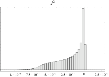
(a) The complete distribution.

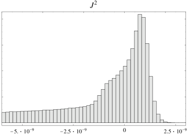
(b) The region $J^{2}\sim 0$.

Figure 1: $J^{2}$ distribution from $\left|V_{us}\right|=0.2200\pm 0.0026$, $\left|V_{cb}\right|=(4.13\pm 0.15)10^{-2}$, $\left|V_{ub}\right|=(3.67\pm 0.47)10^{-3}$ and $\left|V_{cd}\right|=0.224\pm 0.012$.

In order to extract information on $J^{2}$ from the input moduli, it may be tempting to plot only the points that satisfy all unitarity constraints, i.e. normalization of columns and rows of $V_{\mathrm{CKM}}$, together with the constraint of having $J^{2}>0$. We have plotted these points in Fig. 2, which naively lead to $J=\left(2.6\pm 0.8\right)\times 10^{-5}$.

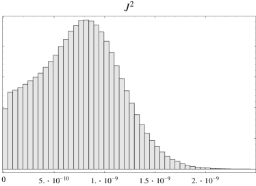
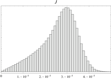
Figure 2: $J^{2}$ and $J$ distributions.

We wish to emphasize that, contrary to what has been stated in the literature [19], one cannot interpret the above result as providing evidence for a complex CKM matrix, using as input data only $\left|V_{us}\right|,\left|V_{cb}\right|,\left|V_{ub}\right|$ and $\left|V_{cd}\right|$. This can be trivially seen from the standard CKM parametrization [20, 21], by noting that from the input moduli $\left|V_{us}\right|,\left|V_{cb}\right|$ and $\left|V_{ub}\right|$, $s_{12},s_{23}$ and $s_{13}$ can be obtained. In order to conclude that $\left|V_{cd}\right|$ has necessarily a non-vanishing contribution proportional to $\cos\delta_{13}$ (the leading one sensitive to $\delta_{13}$), one would need to know $\left|V_{cd}\right|$ with a relative error of $\leq 10^{-4}$ ! It is interesting to point out that the leading contribution to $\left|V_{cd}\right|$ comes from $\left|V_{us}\right|$, therefore also $\left|V_{us}\right|$ would have to be known with the same level of precision, but not $\left|V_{ub}\right|$ and $\left|V_{cb}\right|$. For completeness we plot in Fig. 3(a) the value of $J^{2}$ extracted from input moduli that are assumed to have the required unrealistic precision. It is clear that now, essentially all points have $J^{2}>0$, and therefore the corresponding $J=\left(3.2\pm 0.5\right)\times 10^{-5}$ has full meaning. Figure 3(b) shows the $J^{2}$ distribution obtained with the same inputs as in Fig. 3(a), except for the central value of $\left|V_{cd}\right|$; in this case only $0.16$% of the points have $J^{2}>0$. Notice that both values, $\left|V_{cd}\right|=0.21985\pm 0.00002$ and $\left|V_{cd}\right|=0.21955\pm 0.00002$, are fully compatible with present measurements ($\left|V_{cd}\right|=0.224\pm 0.012$). These two figures clearly show the required precision in $\left|V_{us}\right|$ and $\left|V_{cd}\right|$ to check 3$\times$3 unitarity and to have an irrefutable proof of a complex CKM.

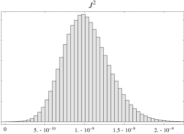
(a) $\left|V_{cd}\right|=0.21985\pm 0.00002$

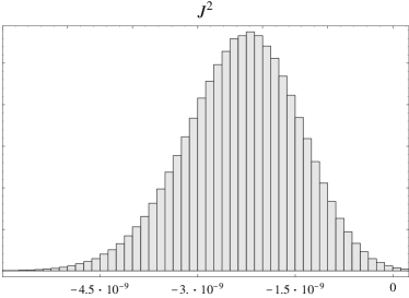
(b) $\left|V_{cd}\right|=0.21955\pm 0.00002$

Figure 3: $J^{2}$ distributions assuming the unrealistic precision values $\left|V_{us}\right|=0.22000\pm 0.00002$ and $\left|V_{cd}\right|$.

Finally, it should be also emphasized that although the above analysis was made using the almost collapsed unitarity triangle corresponding to the first two rows of $V_{\mathrm{CKM}}$, the same conclusions can be obtained if we consider the “standard triangle”, corresponding to orthogonality of the first and third columns. One can evaluate any of the angles of the unitarity triangle in terms of the input moduli, obtaining for example:

$$\sin^{2}\frac{\gamma}{2}=\frac{\left|V_{td}\right|^{2}\left|V_{tb}\right|^{2}-\left(\left|V_{cd}\right|\left|V_{cb}\right|-\left|V_{ud}\right|\left|V_{ub}\right|\right)^{2}}{4\left|V_{ud}\right|\left|V_{ub}\right|\left|V_{cd}\right|\left|V_{cb}\right|}~{},$$ (4)

Since we are using as input moduli $\left|V_{us}\right|$, $\left|V_{cb}\right|$, $\left|V_{ub}\right|$ and $\left|V_{cd}\right|$, it has to be understood that in Eq. (4) one has:

$$\begin{array}[]{c}\left|V_{tb}\right|^{2}=1-\left|V_{cb}\right|^{2}-\left|V_{ub}\right|^{2}~{},\\ \left|V_{td}\right|^{2}=\left|V_{us}\right|^{2}-\left|V_{cd}\right|^{2}+\left|V_{ub}\right|^{2}~{},\\ \left|V_{ud}\right|^{2}=1-\left|V_{us}\right|^{2}-\left|V_{ub}\right|^{2}~{}.\end{array}$$ (5)

The resulting expression can be easily written in terms of the input moduli as:

$$\cos\gamma=\frac{\left|V_{cd}\right|^{2}\left(1-\left|V_{ub}\right|^{2}\right)-\left|V_{us}\right|^{2}\left(1-\left|V_{cb}\right|^{2}\right)+\left|V_{ub}\right|^{2}\left|V_{cb}\right|^{2}}{2\left|V_{ub}\right|\left|V_{cd}\right|\left|V_{cb}\right|\sqrt{1-\left|V_{us}\right|^{2}-\left|V_{ub}\right|^{2}}}~{}.$$ (6)

It is obvious that a “legitimate” extraction of $\gamma$ from the input moduli would require an unrealistic precision in the determination of the chosen moduli. In particular, the difference $\left|V_{cd}\right|^{2}-\left|V_{us}\right|^{2}$ would have to be known at the level of $\left|V_{us}\right|^{2}\left|V_{cb}\right|^{2}$, thus requiring $\left|V_{cd}\right|$ and $\left|V_{us}\right|$ to be measured with a $10^{-4}$ relative error. This confirms our previous argument, based on the standard parametrization. Of course, Eq. (4) can be used to determine $\sin^{2}\gamma/2$ if one uses as input moduli $\left|V_{us}\right|$, $\left|V_{ub}\right|,\left|V_{cb}\right|$ and $\left|V_{td}\right|$. However, $\left|V_{td}\right|$ has the disadvantage that its extraction from experimental data is affected by the possible presence of NP. We will turn to this question in the next section.

Above, we have argued that, although possible in theory, it is not viable in practice to prove that $V_{\mathrm{CKM}}$ is non-trivially complex, from the knowledge of four independent moduli belonging to the first two rows of $V_{\mathrm{CKM}}$. We emphasize that this would be the ideal proof, since the extraction from experiment of the moduli of the first two rows is essentially immune to the possible presence of NP.

4 The impact of $\boldsymbol{\Delta M_{B_{d}}}$ and $\boldsymbol{a_{J/\Psi K_{S}}}$ and the NP parametrization

The experimental measurement of the $B_{d}^{0}$–$\bar{B}_{d}^{0}$ oscillation frequency has reached an average accuracy of almost $1\%$ . The theoretical prediction of $\Delta M_{B_{d}}$ within the SM is given by:

$$\Delta M_{B_{d}}=2\left|M_{12}\right|=\frac{G_{F}^{2}M_{W}^{2}}{6{\pi}^{2}}\eta_{B_{d}}m_{B_{d}}B_{B_{d}}f^{2}_{B_{d}}S_{0}(x_{t})\left|V_{tb}^{\phantom{\ast}}V_{td}^{\ast}\right|^{2}\ ,$$ (7)

where we have followed the standard notation. Equation (7) is an approximation valid up to order $S_{0}(x_{c},x_{t})/S_{0}(x_{t})\sim 10^{-3}$. From this expression we can extract $\left|V_{tb}^{\phantom{\ast}}V_{td}^{\ast}\right|$. Furthermore, unitarity and the experimental values of $\left|V_{ub}\right|$ and $\left|V_{cb}\right|$ determine $\left|V_{tb}\right|$, thus allowing the extraction of $\left|V_{td}\right|$. In Fig. 4 we plot the new $J^{2}$ distribution obtained with $\left|V_{td}\right|$, thus determined together with $\left|V_{us}\right|$, $\left|V_{cb}\right|$ and $\left|V_{ub}\right|$. Table 3 presents all the values used for the input parameters.

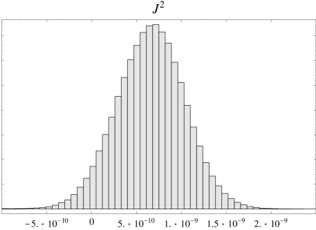
Figure 4: $J^{2}$ distribution obtained with $\left|V_{us}\right|$, $\left|V_{cb}\right|$, $\left|V_{ub}\right|$ and $\left|V_{td}\right|$ (extracted from $\Delta M_{B_{d}}$).

There is a striking difference between Fig. 4 and Fig. 1. As we have emphasized in the previous section, the majority of points obtained for $J^{2}$, when one uses as input $\left|V_{us}\right|$, $\left|V_{cb}\right|$, $\left|V_{ub}\right|$, $\left|V_{cd}\right|$, do not satisfy the unitarity condition that the $uc$ triangle closes (i.e. $J^{2}>0$). On the contrary, when we use $\left|V_{us}\right|$, $\left|V_{cb}\right|$, $\left|V_{ub}\right|$, $\left|V_{td}\right|$ to extract $J^{2}$, the majority of the points satisfies the unitarity condition that $J^{2}>0$ and in fact the value of $\left|J\right|$ agrees with its experimental value $\left|J\right|\sim 10^{-5}$ (of course, using exclusively moduli of $V_{\mathrm{CKM}}$ one cannot determine the sign of $J$). This means that, within the SM, one can use information on $\left|V_{ub}\right|/\left|V_{cb}\right|$ and $\Delta M_{B_{d}}$ to conclude that the triangle cannot collapse to a line, thus implying a complex CKM matrix. Unfortunately, this is not an irrefutable proof that CKM is complex, since $\Delta M_{B_{d}}$ can receive significant contributions from NP, as we have emphasized in section 3. The same is true for the CP asymmetry $a_{J/\Psi K_{S}}$ in the $B_{d}^{0},\bar{B}_{d}^{0}\to J/\Psi K_{S}$ decays. Let us introduce the following parametrization of the NP contribution to $B_{d}^{0}$–$\bar{B}_{d}^{0}$ mixing:

$$M_{12}=r_{d}^{2}e^{-i2\phi_{d}}[M_{12}]_{\mathrm{SM}}$$ (8)

where $[M_{12}]_{\mathrm{SM}}$ is the SM box diagram contribution. The NP contribution to $M_{12}$ implies that $a_{J/\Psi K_{S}}$ no longer measures $2\beta$, but one has instead:

$$a_{J/\Psi K_{S}}=\sin 2(\beta-\phi_{d})=\sin 2\overline{\beta}~{}.$$ (9)

Although the expression for $[M_{12}]_{\mathrm{SM}}$ is the one given by the SM, its actual numerical value may differ from the SM prediction, since models beyond the SM allow in general for a different range of the CKM matrix elements.

It is clear that allowing for the presence of NP in $M_{12}$, parametrized as in Eq. (8), one can fit the data on $a_{J/\Psi K_{S}}$, $\Delta M_{B_{d}}$, even with a real CKM matrix, by putting:

$$\beta=0;\qquad\sin(2\phi_{d})=-a_{J/\Psi K_{S}}$$ (10)

and then adjusting $r_{d}$ to fit $\Delta M_{B_{d}}$. Obviously, two solutions are obtained for $r_{d}$, corresponding to the two ways the unitarity triangle can collapse (i.e. $\gamma=0$ or $\gamma=\pi$). It must be stressed that to write Eq. (9) one has to assume that the potential NP contamination to the penguin diagram contributing to the decay amplitude is negligible. This process is dominated by a tree and a penguin with the same phase; therefore, in this particular case, it is natural to assume no NP in the decay amplitude. For very small deviations from these assumptions see [22].

Independently of the question of whether the CKM matrix is complex or not, it is interesting to investigate what the allowed values for $r_{d}$, $\phi_{d}$ are, taking into account the present data, summarized in Table 3. We calculate, using again the Monte Carlo method, probability density distributions for CKM parameters, $r_{d}^{2}$ and $2\phi_{d}$ using as constraints Gaussian distributions for moduli of the first two rows of the CKM matrix, $\Delta M_{B_{d}}$ and $a_{J/\Psi K_{S}}$. In Fig. 5(a) we plot 68% (black), 90% (dark grey) and 95% (grey) probability regions of the probability density function (PDF) of the apex $-V_{ud}^{\phantom{\ast}}V_{ub}^{\ast}/V_{cd}^{\phantom{\ast}}V_{cb}^{\ast}$ of the $db$ unitarity triangle. In Fig. 5(b) we represent joint PDF regions in the plane $(r^{2}_{d}$, $2\phi_{d})$. Because $\gamma$ gives the apex of the triangle, it is clear from Fig. 5(a) that there is essentially no restriction on $\gamma$. On the contrary, because the moduli of the first two rows put an upper bound on $|\beta|$ and upper and lower bounds on $R_{t}=\left|V_{td}^{\phantom{\ast}}V_{tb}^{\ast}\right|/\left|V_{cd}^{\phantom{\ast}}V_{cb}^{\ast}\right|$, we can see in Fig. 5(b) significant constraints on $2\phi_{d}$ and $r_{d}^{2}$. Although the experimental value of the semileptonic asymmetry $A_{\mathrm{SL}}$ (the asymmetry in the number of equal sign lepton pairs arising from the semileptonic decay of $B_{d}^{0}$–$\bar{B}_{d}^{0}$ pairs) has some impact on these figures, we have not included it in order to show in a clear way the impact of the actual measurements. We will come back to this point later on.

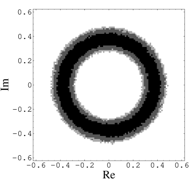
(a) Apex $-\frac{V_{ud}V_{ub}^{\ast}}{V_{cd}V_{cb}^{\ast}}$ of the unitarity triangle $db$.

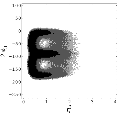
(b) $(r_{d}^{2},2\phi_{d})$ joint distribution.

Figure 5: 68%(black), 90%(dark grey) and 95%(grey) probability regions.

At this stage, the following comment is in order. We are assuming a class of theories beyond the SM that give NP contributions to $\Delta M_{B_{d}}$, but keep $V_{\mathrm{CKM}}$ unitary. The most important example of this class of theories are the supersymmetric extensions of the SM. Since in this framework $V_{\mathrm{CKM}}$ is still unitary, once $\left|V_{us}\right|$, $\left|V_{cb}\right|$, $\left|V_{ub}\right|/\left|V_{cb}\right|$ are fixed by data, there is only $\beta$ as a free independent CKM parameter. It is then clear that with only two experimental inputs, namely $\Delta M_{B_{d}}$, $a_{J/\Psi K_{S}}$, one cannot fix the three parameters $r_{d}$, $\phi_{d}$, $\beta$. One may be tempted to include information on $\Delta M_{B_{s}}$. However, in our scenario, this would require the introduction of new parameters ($r_{s}$, $\phi_{s}$) giving NP contributing to $\Delta M_{B_{s}}$.

In the next section, we will emphasize the importance of $\gamma$ in obtaining an irrefutable proof that $V_{\mathrm{CKM}}$ is complex, even allowing for the presence of NP.

5 The importance of a direct measurement of the phase $\boldsymbol{\gamma}$

In our framework, we can distinguish two conceptually different ways of measuring $\gamma$ in $B_{d}^{0}$ non-leptonic decays: those that come from the interference of two tree-level decays such as $b\rightarrow s\bar{u}c$ with $b\rightarrow s\bar{c}u$, or $b\rightarrow d\bar{u}c$ with $b\rightarrow d\bar{c}u$, and those other processes where the presence of both tree and penguin diagrams is allowed, such as $b\rightarrow d\bar{u}u$ interfering with $b\rightarrow d$. The first group includes the usual methods that are called, in the literature, methods to measure $\gamma$ or $2\overline{\beta}+\gamma$ [23, 24]. In general they involve the transitions $B\rightarrow DK$ or $B\rightarrow D\pi$ as the flavour-representative examples of the considered decays. The second group includes the usual methods to measure $\alpha$ [25, 26], or more generally $\overline{\alpha}=\pi-\overline{\beta}-\gamma$ if one allows for the presence of NP in $B_{d}^{0}$–$\bar{B}_{d}^{0}$ mixing. By now it is well known that the so-called methods to measure $\overline{\alpha}$ in fact ought to be called methods to measure $\overline{\beta}+\gamma$ [27, 28]. Of course, the representative example of this method as far as flavour content is concerned is $B\rightarrow\pi\pi$.

It has to be stressed that there are other available methods to extract $\gamma$, i.e. using $b\rightarrow s$ transitions. However, in the search for NP, great attention has to be payed to the assumptions made in order to keep the errors under control. In this respect, $SU(2)$ is a very good symmetry of the strong interactions, but the same does not hold for $SU(3)$. Furthermore, there are no first principle calculations of $SU(3)$ breaking effects in non-leptonic $B$-decays. Therefore, although analyses based on $SU(3)$, $U$-spin, can be quite useful in some instances, we will restrict ourselves to $SU(2)$-based analyses, as far as strong interactions are concerned.

Concerning the two previous methods, their fundamental differences lie in the presence or not of penguin diagrams. The method to extract $\gamma$ or $2\overline{\beta}+\gamma$ relies on pure tree-level processes, therefore no additional assumptions are needed to get a value of $\gamma\neq 0$ so as to have an irrefutable proof for a complex $V_{\mathrm{CKM}}$. Of course it has to be understood that $2\overline{\beta}$ has been extracted from ${B}_{d}^{0},\bar{B}_{d}^{0}\rightarrow J/\Psi K_{S},J/\Psi{K}^{0\ast},J/\Psi\bar{K}^{0\ast}$ in order to use the method of the $2\overline{\beta}+\gamma$ extraction. In the $\overline{\alpha}$ method, the presence of penguins in general calls for the additional assumption of no NP competing with these penguins in the decay amplitudes. Therefore we will present two separate analyses with the actual relevant data.

5.1 $\boldsymbol{\gamma}$ from pure weak tree-level decays

The enormous effort developed at the B-factories Belle and BaBar has resulted in the first measurements of $\gamma$ – although by now still poor – in tree-level decays $B^{\pm}\rightarrow DK^{\pm}$, $B^{\pm}\rightarrow D^{\ast}K^{\pm}\rightarrow\left(D\pi^{0}\right)K^{\pm}$, where the two paths to $D^{0}$ or $\bar{D}^{0}$ interfere in the common decay channel $\bar{D}^{0},{D}^{0}\rightarrow K_{S}\pi^{+}\pi^{-}$. From a Dalitz-plot analysis [29], Belle has presented $\gamma=68^{\circ}\pm\begin{smallmatrix}14^{\circ}\\ 15^{\circ}\end{smallmatrix}\pm 13^{\circ}\pm 11^{\circ}$ and BaBar [30] $\gamma=70^{\circ}\pm 26^{\circ}\pm 10^{\circ}\pm 10^{\circ}$, together with the solutions obtained by changing $\gamma\rightarrow\gamma\pm\pi$. The statistical significance of CP violation in the Belle measurement is of $98\%$ [29]; by now therefore this can be taken as an indicative figure of the statistical significance of having a complex CKM.

The method used by Belle and BaBar suffers from model-dependent assumptions in the Dalitz-plot analysis; these can be eliminated with more statistics following the suggestion of Ref. [24]. Also, the presence of NP in the $D^{0}$–$\bar{D}^{0}$ mixing could modify this analysis, but if necessary, in case of better precision, this small correction [24] could be included in the way suggested in Refs. [31].

We average conservatively both measurements to the value $\gamma=69^{\circ}\pm 21^{\circ}$ ($-111^{\circ}\pm 21^{\circ}$), which we take as a quantitative measurement of a complex CKM matrix independent of the presence of NP at the one-loop weak level. To analyse the implications for the presence of NP, we add this new constraint to the previous analysis presented in Figs. 5(a) and 5(b). In Fig. 6(a) we represent the analogue of Fig. 5(a). From Table 1, where we only present the central values, we clearly see that with two $\gamma$ values and two signs for $\cos(2\overline{\beta})$ we generate four solutions.

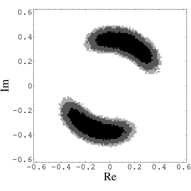
(a) Apex $-\frac{V_{ud}V_{ub}^{\ast}}{V_{cd}V_{cb}^{\ast}}$ of the unitarity triangle $db$.

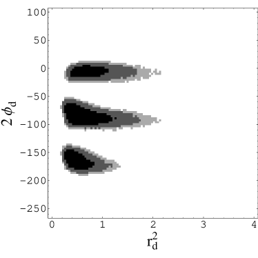
(b) $(r_{d}^{2},2\phi_{d})$ joint distribution.

Figure 6: 68% (black), 90% (dark grey) and 95% (grey) probability regions, including the constraint on $\gamma$.

It has to be stressed that although $\overline{\beta}$ presents a fourfold ambiguity, $2\overline{\beta}$ – necessary to extract $2\phi_{d}$ – presents a twofold one. With a measurement of $\gamma$ (another twofold ambiguity) we have $\beta$ and $R_{t}$ fixed up to a twofold ambiguity, and therefore in total we have four different solutions for $r_{d}^{2}$, $2\phi_{d}$ and the CKM parameters.

These solutions are represented in the $(r_{d}^{2},2\phi_{d})$ plane as the joint PDF in Fig. 6(b). We have the “SM solution” corresponding to $2\phi_{d}\sim 0^{\circ}$, $r_{d}\sim 1$, two NP solutions overlapping at $2\phi_{d}\sim-85^{\circ}$ and another NP solution near $2\phi_{d}\sim-169^{\circ}$. Had we used the constraint on the sign of $\cos(2\overline{\beta})$, from $B_{d}^{0}\rightarrow J/\Psi K^{\ast}$, we would have eliminated two NP solutions, but the situation is not conclusive (see [32]). The fact that the central value of $\gamma$ is a little bit high with respect to the value obtainable in a SM fit, implies a large value for $R_{t}$ for the “SM solution”, and therefore a low central value of $r_{d}$, i.e. $r_{d}^{2}<1$.

Information on $2\overline{\beta}+\gamma$ is also available from partially reconstructed $B^{0}\rightarrow D^{\ast\pm}\pi^{\mp}$ decays, $\left|\sin\left(2\overline{\beta}+\gamma\right)\right|>0.58$ (90% C.L.) [33]. But at the moment this result relies on theoretical inputs based on $SU(3)$, and we will therefore not use this constraint. Coming back to our irrefutable proof of a complex CKM, with our PDF for $\gamma$ we find that a real CKM matrix is excluded at a 99.84% C.L.. In much more intuitive terms, we find that the probability corresponding to $\gamma\in[10^{\circ};170^{\circ}]\cup[-170^{\circ};-10^{\circ}]$ is 99.7%.

$\gamma$ (input)	$\beta$	$2\phi_{d}$	$r_{d}^{2}$	$R_{t}$	Sign[cos($2\overline{\beta}$)]	$2\overline{\beta}$ (input)	$\overline{\alpha}$
$69^{\circ}$	$23.2^{\circ}$	$-0.8^{\circ}$	$0.80$	$0.93$	+	$47.2^{\circ}$	$87.4^{\circ}$
$69^{\circ}$	$23.2^{\circ}$	$-86.4^{\circ}$	$0.80$	$0.93$	-	$132.8^{\circ}$	$44.6^{\circ}$
$-111^{\circ}$	$-17.9^{\circ}$	$-83.0^{\circ}$	$0.48$	$1.20$	+	$47.2^{\circ}$	$-92.6^{\circ}$
$-111^{\circ}$	$-17.9^{\circ}$	$-168.6^{\circ}$	$0.48$	$1.20$	-	$132.8^{\circ}$	$-135.4^{\circ}$

Table 1: “Central” values for the solutions (see Fig. 6).

5.2 $\boldsymbol{\gamma}$ from $\boldsymbol{\overline{\alpha}}$ methods

Using these $\overline{\alpha}$ methods to get an irrefutable proof of a complex $V_{\mathrm{CKM}}$ is in principle much more subtle. They are all based on the transition $b\rightarrow du\bar{u}$, so that the so-called penguin pollution (weak loops) can also become NP pollution. The most prominent channels are $B\rightarrow\pi\pi$, $B\rightarrow\rho\pi$ and $B\rightarrow\rho\rho$. In the appendix we have shown that the extraction of $\overline{\alpha}=\pi-\overline{\beta}-\gamma=\alpha+\phi_{d}$ from these channels is valid even in the presence of any NP in the $\Delta I=1/2$ piece of the weak hamiltonian. As the $\Delta I=3/2$ piece is dominated by tree diagrams, this extraction of $\overline{\alpha}$ is in accordance with our initial assumptions: “no NP in weak processes where the SM contributes at tree level” means in this case no NP in the $\Delta I=3/2$ piece. We conclude that the extraction of $\overline{\alpha}$ from these channels is completely independent of the presence of NP in the usual penguins. Only NP in electroweak penguins (EWP) could spoil this conclusion, but this is very unlikely due to the small effect of the SM EWP, of order $1.5^{\circ}$ (see reference [35]), that can be eventually taken into account.

BaBar has presented a time-dependent analysis of the $\rho^{+}\rho^{-}$ channel [36], that once supplemented with the $\rho^{+}\rho^{0}$ and $\rho^{0}\rho^{0}$ branching ratios [37, 38] and the measurement of the final polarization [36], can be translated [39] into the measured value $\overline{\alpha}=96^{\circ}\pm 10^{\circ}\pm 5^{\circ}\pm 11^{\circ}$ where the last error comes from the usual $SU(2)$ isospin bounds $\left|\overline{\alpha}_{\mathrm{eff}}-\overline{\alpha}\right|\leq 11^{\circ}$. Because the measurement is sensitive to $\sin(2\overline{\alpha}_{\mathrm{eff}})$, $\overline{\alpha}=\overline{\alpha}_{\mathrm{eff}}\pm 11^{\circ}$ presents a fourfold ambiguity $\left(\overline{\alpha},\overline{\alpha}+\pi,\frac{\pi}{2}-\overline{\alpha},-\overline{\alpha}-\frac{\pi}{2}\right)$. In the $\rho\pi$ channel the pentagon isospin analysis – from quasi-two-body decays – needs more statistics and/or additional assumptions. A time-dependent Dalitz-plot analysis in the channel $B\rightarrow\pi^{+}\pi^{-}\pi^{0}$ has been presented by BaBar [37, 40], with the result $\overline{\alpha}=113^{\circ}\pm\begin{smallmatrix}27^{\circ}\\ 17^{\circ}\end{smallmatrix}\pm 6^{\circ}$.

Since this analysis is sensitive to both $\sin\left(2\overline{\alpha}_{\mathrm{eff}}\right)$ and $\cos\left(2\overline{\alpha}_{\mathrm{eff}}\right)$, the resulting ambiguity is just a twofold one $\left(\overline{\alpha},\overline{\alpha}+\pi\right)$. It is remarkable that these two solutions are in good agreement with two of the solutions coming from the $\rho\rho$ channel. This important property will be used to eliminate two of the four solutions coming from the $\rho\rho$ channel, in order to see the future trend of this analysis in a much clearer way.

The situation in the $\pi\pi$ channel does not yet allow a full isospin analysis and the isospin bounds are quite poor. Furthermore BaBar and Belle measurements are still in some conflict, so that we will not use these results.

As before, we average the data from $\rho\rho$ and $\rho\pi$ but only keep the two solutions consistent with the $\rho\pi$ channel data. Our averaged values are $\overline{\alpha}=100^{\circ}\pm 16^{\circ}$, ($-80^{\circ}\pm 16^{\circ}$).

The analogue of Fig. 6(a) for the apex of the unitarity triangle, with the information on $\gamma$ replaced by that on $\overline{\alpha}$, is represented in Fig. 7(a).

In this case the data are not conclusive enough to eliminate a real $V_{\mathrm{CKM}}$; a real CKM is excluded at a 75% C.L.. In the second approach, the probability of $\gamma\in[10^{\circ};170^{\circ}]\cup[-170^{\circ};-10^{\circ}]$ is 85%. In Table 2, where we include the central values, we have four solutions from the two $\overline{\alpha}$ values and the two signs of $\cos(2\overline{\beta})$. Again, the fourfold $\overline{\beta}$ ambiguity is effectively reduced to two because to reconstruct $\gamma$, the quantity that matters is $(\overline{\alpha}+\overline{\beta})=\pi-\gamma$. These solutions are represented in Fig. 7(b). As before, we have the SM solution and the other three NP solutions that tend to overlap here more than in the previous case.

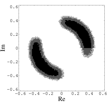
(a) Apex $-\frac{V_{ud}V_{ub}^{\ast}}{V_{cd}V_{cb}^{\ast}}$ of the unitarity triangle $db$.

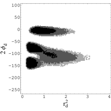
(b) $(r_{d}^{2},2\phi_{d})$ joint distribution.

Figure 7: 68% (black), 90% (dark grey) and 95% (grey) probability regions, including the constraint on $\gamma$ through $\overline{\alpha}$.

$\gamma$	$\beta$	$2\phi_{d}$	$r_{d}^{2}$	$R_{t}$	Sign[cos($2\overline{\beta}$)]	$2\overline{\beta}$ (Input)	$\overline{\alpha}$ (Input)
$56.4^{\circ}$	$22.8^{\circ}$	$-1.7^{\circ}$	$0.96$	$0.85$	+	$47.2^{\circ}$	$100^{\circ}$
$13.6^{\circ}$	$8.5^{\circ}$	$-115.7^{\circ}$	$1.78$	$0.62$	-	$132.8^{\circ}$	$100^{\circ}$
$-123.6^{\circ}$	$-15.1^{\circ}$	$-77.4^{\circ}$	$0.44$	$1.26$	+	$47.2^{\circ}$	$-80^{\circ}$
$-166.4^{\circ}$	$-3.8^{\circ}$	$-140.5^{\circ}$	$0.36$	$1.39$	-	$132.8^{\circ}$	$-80^{\circ}$

Table 2: “Central” values for the solutions (see Fig. 7).

Comparing the two tables and taking errors into account, it is easy to recognize that the two solutions with positive sign of $\cos(2\overline{\beta})$ can be consistent, but the negative ones are somewhat inconsistent. The reason can be seen by looking at the $\overline{\alpha}$ generated from the $\gamma$ measurement. Because $\overline{\alpha}=\pi-\overline{\beta}-\gamma$, the two $\overline{\alpha}$ generated with the same $\overline{\beta}$ (the same sign of $\cos(2\overline{\beta})$) differ by $\pi$, so if one of the $\gamma$ measurements is consistent with one of the $\overline{\alpha}$ measurements, so is the other, because both measurements of $\overline{\alpha}$ and $\gamma$ differ by $\pi$. On the contrary, for a fixed $\gamma$ measurement, the two $\overline{\alpha}$ generated with the different $\overline{\beta}$ (different sign of $\cos(2\overline{\beta})$) differ by $42.8^{\circ}$, so if one solution is compatible with the $\overline{\alpha}$ measurement, the other is not. In our scenario, therefore, a way of measuring the sign of $\cos(2\overline{\beta})$ relies on the measurements of $\sin(2\overline{\beta})$, $\sin(2\overline{\alpha})$, $\cos(2\overline{\alpha})$ and $\tan\gamma$.

In Fig. 8 we repeat the previous analyses including both constraints from $\gamma$ and $\overline{\alpha}$. As can be seen the solutions with negative $\cos(2\overline{\beta})$ have almost disappeared, in fact just $11.1\%$ of the points have negative $\cos(2\overline{\beta})$, contrary to the previous plots, where they were $50\%$. Combining $\gamma$ and $\overline{\alpha}$ measurements, a real CKM matrix is excluded at a 99.92% C.L. and the probability of $\gamma\in[10^{\circ};170^{\circ}]\cup[-170^{\circ};-10^{\circ}]$ is 99.7%.

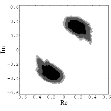
(a) Apex $-\frac{V_{ud}V_{ub}^{\ast}}{V_{cd}V_{cb}^{\ast}}$ of the unitarity triangle $db$.

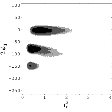
(b) $(r_{d}^{2},2\phi_{d})$ joint distribution.

Figure 8: 68% (black), 90% (dark grey) and 95% (grey) probability regions, including the constraints on $\gamma$ derived from both direct $\gamma$ measurements as well as from $\overline{\alpha}$.

As we have mentioned, previous work on these analyses of New Physics has been presented by Z. Ligeti in [15]. For similar experimental inputs and theoretical assumptions the results agree.

5.3 Further comments

The semileptonic asymmetry is $A_{\mathrm{SL}}=\text{Im}\left(\Gamma_{12}/M_{12}\right)$, where in our scenario $M_{12}$ is polluted by NP, $M_{12}=\frac{1}{2}\Delta M_{B_{d}}e^{i2\overline{\beta}}$, but – to the present level of precision – $\Gamma_{12}\propto(a+be^{-i\gamma}+ce^{-i2\gamma})$ is not; $a,b,c$ depend on QCD parameters and moduli of the first two rows of the CKM matrix [41, 42, 14]. Therefore, by including the measurements of $\Delta M_{B_{d}}$, $a_{J/\Psi K_{S}}$ and a determination of the sign of $\cos(2\overline{\beta})$, $A_{\mathrm{SL}}$ could be used in the future to obtain information on $\gamma$. The impact of the actual value $A_{\mathrm{SL}}=(-3\pm 7)\times 10^{-3}$ [44] in Figs. 6, 7 and 8 is very mild, but a future determination of $A_{\mathrm{SL}}$ at the level of the SM precision ($A_{\mathrm{SL}}^{\mathrm{SM}}=(-5.0\pm 1.1)\times 10^{-4}$ [41] ) would be sufficient by itself to completely eliminate some $\gamma$ solutions.

In some parts of our analyses we have used 3$\times$3 unitarity. It is important to clarify that a direct measurement of $\gamma$ from tree-level decays (or in the future from $A_{\mathrm{SL}}$) provides an irrefutable proof of a complex CKM matrix, independent of violations of 3$\times$3 unitarity; this includes both $\gamma$ and $\overline{\alpha}$ methods. This is not the case of our analyses of NP, where we have extensively used 3$\times$3 unitarity, for example in the extraction of $\beta$ and $R_{t}$ from moduli of the first two rows and $\gamma$ so as to obtain $2\phi_{d}$ and $r_{d}^{2}$.

6 Summary and Conclusions

We have carefully examined the present experimental evidence in favour of a complex CKM matrix, even allowing for NP contributions to $\epsilon_{K}$, $\Delta M_{B_{d}}$, $\Delta M_{B_{s}}$, $a_{J/\Psi K_{S}}$, $B\to\rho\rho$ and $B\to\rho\pi$. First, we showed that, contrary to some statements in the literature [19], it is not feasible in practice to derive a non-vanishing value of $|J|$ using only the present information on moduli of the first two rows of the CKM matrix. We showed this by pointing out that a legitimate determination of $|J|$ from these moduli, although possible in theory, would in practice require a completely unrealistic high-precision determination of $\left|V_{us}\right|$, $\left|V_{cd}\right|$. We then introduced a convenient parametrization of NP and examined the impact of $\Delta M_{B_{d}}$ and $a_{J/\Psi K_{S}}$ in obtaining experimental evidence of a complex CKM matrix. We then emphasized that the best evidence for CKM to be complex, arises from $\gamma$, either through a direct measurement or through a measurement of $\overline{\alpha}$, together with $\overline{\beta}$. We conclude that if NP does not pollute SM amplitudes dominated by tree level diagrams, a real CKM is excluded at a 99.92% C.L., and the probability of having $\gamma$ in the region $[10^{\circ};170^{\circ}]\cup[-170^{\circ};-10^{\circ}]$ is 99.7%. We also illustrated how the above measurements can be used to place limits on the size of NP, which is allowed by the present data. As we emphasized in the Introduction, having an irrefutable piece of evidence for a complex CKM matrix, in a framework where the presence of NP is allowed, has profound implications for models of CP violation. In the particular case of models with spontaneous CP violation, a complex CKM matrix favours the class of models [5], [6] where, although Yukawa couplings are real, the vacuum phase responsible for spontaneous CP violation also generates CP violation in charged-current weak interactions. Conversely, the evidence for a complex CKM matrix, even allowing for the presence of NP, excludes the class of models with spontaneous CP violation and a real CKM matrix at a 99.92% C.L..

Appendix

In this appendix we explain why the extraction of $\overline{\alpha}$ based in the so-called isospin analysis is valid even in the presence of New Physics in the $\Delta I=1/2$ piece of the $b\to d$ hamiltonian. This is true for $B\to\pi\pi$, $B\to\rho\rho$ and $B\to\rho\pi$.

In the $B\to\pi\pi$ case, as has been rephrased in [43], the basic ingredients to extract $\overline{\alpha}$ are:

• The full hamiltonian only contains $\Delta I=1/2,3/2$ pieces, and isospin is a good symmetry of final state interactions. With these ingredients one has

  $$\lambda_{+0}\equiv\frac{q}{p}\frac{\overline{A}_{+0}}{A_{+0}}=e^{-i2\overline{\beta}}\frac{\overline{A}_{3/2}}{A_{3/2}}~{},$$ (11)

  and $\lambda_{+0}$ is a “physical observable” that can be reconstructed (up to discrete ambiguities) with the directly measurable observables $\lambda_{+-}=\frac{q}{p}\frac{\overline{A}_{+-}}{A_{+-}}$ and the branching ratios of the 6 available channels $B^{i+j}\to\pi^{i}\pi^{j}$ and their CP-conjugates; obviously $A_{+0}=A(B^{+}\to\pi^{+}\pi^{0})\propto A_{3/2}$ and $A_{+-}=A(B^{0}\to\pi^{+}\pi^{-})$.

• If the $\Delta I=3/2$ piece of the hamiltonian is exactly the SM one (the tree level piece ) we have

  $$\lambda_{+0}=e^{-i2\overline{\beta}}e^{-i2\gamma}=e^{+i2\overline{\alpha}}~{}.$$ (12)

It is important to stress that the extraction of $\lambda_{+0}$ is valid in any model of NP that fulfills assumption (i), therefore the extraction of $\overline{\alpha}$ from equation (12) is valid in any model where the NP in the decay amplitudes only appears in the $\Delta I=1/2$ piece. If full isospin analysis is not done, because the usual bounds are obtained assuming (i), the result is also valid. The $B\to\rho\rho$ case is similar to the $B\to\pi\pi$ case.

In the Dalitz plot analysis of $B\to\rho\pi$, the moduli and the relative phases of $A^{+-}=A(B^{0}\to\rho^{+}\pi^{-})$, $A^{-+}=A(B^{0}\to\rho^{-}\pi^{+})$ and $A^{00}=A(B^{0}\to\rho^{0}\pi^{0})$, are measured, together with the CP-conjugate channels, and a global relative phase weighted by $q/p$. With a general weak hamiltonian $H_{w}$ with $\Delta I=1/2,3/2$ pieces one obtains from isospin

$$e^{-i2\overline{\beta}}\frac{\overline{A}_{3/2,2}}{A_{3/2,2}}=e^{-i2\overline{\beta}}\frac{\overline{A}^{+-}+\overline{A}^{-+}+2\overline{A}^{00}}{A^{+-}+A^{-+}+2A^{00}}~{},$$ (13)

where $A_{3/2,2}$ is the reduced matrix element of $H_{w}(\Delta I=3/2)$ with a $I=2$ final state. Assuming that $H_{w}(\Delta I=3/2)$ is the SM one, we have

$$e^{-i2\overline{\beta}}\frac{\overline{A}_{3/2,2}}{A_{3/2,2}}=e^{-i2(\overline{\beta}+\gamma)}=e^{i2\overline{\alpha}}~{}.$$ (14)

So the extraction of $\overline{\alpha}$ from the Dalitz plot analysis in $B\to\rho\pi$ is completely valid in the presence of any NP in the $\Delta I=1/2$ hamiltonian.

References

- [1] N. Cabibbo, Phys. Rev. Lett. 10, 531 (1963). M. Kobayashi and T. Maskawa, Prog. Theor. Phys. 49, 652 (1973).
-
[2]
UTfit, M. Bona et al.,
hep-ph/0501199,
http://www.utfit.org CKMfitter Group, J. Charles et al., hep-ph/0406184,
http://ckmfitter.in2p3.fr A. J. Buras, F. Parodi, and A. Stocchi, JHEP 01, 029 (2003), hep-ph/0207101. - [3] G. C. Branco, F. Cagarrinho, and F. Kruger, Phys. Lett. B459, 224 (1999), hep-ph/9904379.
- [4] T. D. Lee, Phys. Rev. D8, 1226 (1973).
- [5] G. C. Branco and M. N. Rebelo, Phys. Lett. B160, 117 (1985). J. Liu and L. Wolfenstein, Nucl. Phys. B289, 1 (1987).
- [6] L. Bento and G. C. Branco, Phys. Lett. B245, 599 (1990). L. Bento, G. C. Branco, and P. A. Parada, Phys. Lett. B267, 95 (1991).
- [7] G. C. Branco, F. Kruger, J. C. Romao, and A. M. Teixeira, JHEP 07, 027 (2001), hep-ph/0012318. C. Hugonie, J. C. Romao, and A. M. Teixeira, JHEP 06, 020 (2003), hep-ph/0304116.
- [8] G. C. Branco, Phys. Rev. Lett. 44, 504 (1980). G. C. Branco, Phys. Rev. D22, 2901 (1980). G. C. Branco, A. J. Buras, and J. M. Gerard, Nucl. Phys. B259, 306 (1985).
- [9] BaBar, B. Aubert et al., Phys. Rev. Lett. 93, 131801 (2004), hep-ex/0407057. Belle, Y. Chao et al., Phys. Rev. Lett. 93, 191802 (2004), hep-ex/0408100.
- [10] G. C. Branco, L. Lavoura and J. P. Silva, “CP violation,” International Series of Monographs on Physics, No. 103, Oxford University Press. Oxford, UK: Clarendon (1999), 511 pp.
- [11] R. Aleksan, B. Kayser, and D. London, Phys. Rev. Lett. 73, 18 (1994), hep-ph/9403341.
- [12] F. J. Botella, G. C. Branco, M. Nebot, and M. N. Rebelo, Nucl. Phys. B651, 174 (2003), hep-ph/0206133. J. A. Aguilar-Saavedra, F. J. Botella, G. C. Branco, and M. Nebot, Nucl. Phys. B706, 204 (2005), hep-ph/0406151.
- [13] J. Silva, and L. Wolfenstein, Phys. Rev. D55, 5331 (1997), hep-ph/9610208.
- [14] CKMfitter Group, J. Charles et al., same as in [2].
- [15] Z. Ligeti, hep-ph/0408267.
- [16] F. J. Botella and L.-L. Chau, Phys. Lett. B168, 97 (1986). G. C. Branco and L. Lavoura, Phys. Lett. B208, 123 (1988).
- [17] C. Jarlskog, Phys. Rev. Lett. 55, 1039 (1985).
- [18] G. Cowan, Oxford, UK: Clarendon, (1998), 197 pp. G. D’Agostini, CERN Report 99-03 (1999). G. D’Agostini, Rep. Prog. Phys. 66, 1383 (2003), physics/0304102.
- [19] M. Randhawa and M. Gupta, hep-ph/0102274. M. Randhawa and M. Gupta, Phys. Lett. B516, 446 (2001), hep-ph/0106161. P. Dita, hep-ph/0408013.
- [20] L.-L. Chau and W.-Y. Keung, Phys. Rev. Lett. 53, 1802 (1984).
- [21] S. Eidelman et al. [Particle Data Group Collaboration], Phys. Lett. B 592, 1 (2004)
- [22] D. Atwood and G. Hiller, hep-ph/0307251.
- [23] M. Gronau and D. London, Phys. Lett. B253, 483 (1991). M. Gronau and D. Wyler, Phys. Lett. B265, 172 (1991). I. Dunietz, Phys. Lett. B270, 75 (1991). R. Aleksan, I. Dunietz, and B. Kayser, Z. Phys. C54, 653 (1992). D. Atwood, G. Eilam, M. Gronau, and A. Soni, Phys. Lett. B341, 372 (1995), hep-ph/9409229. D. Atwood, I. Dunietz, and A. Soni, Phys. Rev. Lett. 78, 3257 (1997), hep-ph/9612433. A. Bondar and T. Gershon, Phys. Rev. D70, 091503 (2004), hep-ph/0409281.
- [24] A. Giri, Y. Grossman, A. Soffer, and J. Zupan, Phys. Rev. D68, 054018 (2003), hep-ph/0303187.
- [25] M. Gronau and D. London, Phys. Rev. Lett. 65, 3381 (1990). Y. Grossman and H. R. Quinn, Phys. Rev. D58, 017504 (1998), hep-ph/9712306. J. Charles, Phys. Rev. D59, 054007 (1999), hep-ph/9806468. M. Gronau, D. London, N. Sinha, and R. Sinha, Phys. Lett. B514, 315 (2001), hep-ph/0105308.
- [26] A. E. Snyder and H. R. Quinn, Phys. Rev. D48, 2139 (1993).
- [27] J. P. Silva, hep-ph/0410351.
- [28] G. Barenboim, F. J. Botella, G. C. Branco, and O. Vives, Phys. Lett. B422, 277 (1998), hep-ph/9709369.
- [29] Belle, K. Abe et al., hep-ex/0411049.
- [30] BaBar, B. Aubert et al., hep-ex/0408088.
- [31] A. Amorim, M. G. Santos, and J. P. Silva, Phys. Rev. D59, 056001 (1999), hep-ph/9807364. C. C. Meca and J. P. Silva, Phys. Rev. Lett. 81, 1377 (1998), hep-ph/9807320. J. P. Silva and A. Soffer, Phys. Rev. D61, 112001 (2000), hep-ph/9912242.
- [32] BaBar, B. Aubert et al., hep-ex/0411016. Belle, K. Abe et al., hep-ex/0408104.
- [33] BaBar, B. Aubert, hep-ex/0408038.
- [34] Private communication, Fernando Martínez Vidal.
- [35] M. Gronau and J. Zupan, Phys. Rev. D71, 074017 (2005), hep-ph/0502139.
- [36] BaBar, B. Aubert et al., Phys. Rev. Lett. 93, 231801 (2004), hep-ex/0404029.
- [37] BaBar, B. Aubert et al., Phys. Rev. Lett. 91, 201802 (2003), hep-ex/0306030.
- [38] Belle, J. Zhang et al., Phys. Rev. Lett. 91, 221801 (2003), hep-ex/0306007.
- [39] BaBar, A. Bevan, hep-ex/0411090.
- [40] BaBar, B. Aubert et al., hep-ex/0408099.
- [41] M. Beneke, G. Buchalla, A. Lenz, and U. Nierste, Phys. Lett. B576, 173 (2003), hep-ph/0307344. M. Ciuchini, E. Franco, V. Lubicz, F. Mescia, and C. Tarantino, JHEP 08, 031 (2003), hep-ph/0308029.
- [42] G. C. Branco, P. A. Parada, T. Morozumi, and M. N. Rebelo, Phys. Lett. B306, 398 (1993). S. Laplace, Z. Ligeti, Y. Nir, and G. Perez, Phys. Rev. D65, 094040 (2002), hep-ph/0202010.
- [43] F.J. Botella and J. Silva, Phys. Rev. D71, 094008 (2005), hep-ph/0503136.
- [44] Heavy Flavour Averaging Group , hep-ex/0412073. http://www.slac.stanford.edu/xorg/hfag/