January, 2005

CERN-PH-TH/2005-012

Pion-pion scattering
and the $K\rightarrow 3\pi\,$ decay amplitudes

Nicola Cabibbo^a,b and Gino Isidori^c

${}^{a}~{}$CERN, Physics Department, CH-1211 Geneva 23, Switzerland

${}^{b}~{}$Dipartimento di Fisica Università di Roma “La Sapienza” and
INFN, Sezione di Roma, P.le A. Moro 2, I-00185 Rome, Italy

${}^{c}~{}$INFN, Laboratori Nazionali di Frascati, I-00044 Frascati, Italy

We revisit the recently proposed method for the determination of the $\pi\pi$ scattering length combination $a_{0}-a_{2}$, based on the study of the $\pi^{0}\pi^{0}\,$ spectrum in $K^{+}\rightarrow\pi^{+}\pi^{0}\pi^{0}\,$. In view of a precision measurement, we discuss here the effects due to smaller absorptive contributions to the $K^{+}\rightarrow\pi^{+}\pi^{0}\pi^{0}\,$ and $K^{+}\rightarrow\pi^{+}\pi^{+}\pi^{-}\,$amplitudes. We outline a method of analysis that can lead to a precision determination of $a_{0}-a_{2}$ and is based on very general properties of the S matrix. The discussion of final-state rescattering and cusp effects is also extended to the two $K_{L}\to 3\pi$ coupled channels. Thanks to the present work, the theoretical error on the $a_{0}-a_{2}$ combination extracted from the $K^{+}\rightarrow\pi^{+}\pi^{0}\pi^{0}\,$ spectrum is reduced to about $5\%$. A further reduction requires the evaluation of the effects arising from radiative corrections.

1 Introduction

In [1] it was shown how rescattering of the final state pions in $K^{+}\rightarrow\pi^{+}\pi^{0}\pi^{0}\,$ produces a prominent cusp in the total energy spectrum of the $\pi^{0}\pi^{0}\,$ pair, whose amplitude is proportional to the $a_{0}-a_{2}$ combination of the $\pi\pi\,$  S-wave scattering lengths.

The combination $a_{0}-a_{2}$ is a very interesting quantity: a benchmark observable to determine the structure of the QCD vacuum and one of the few non-perturbative parameters which can be predicted with excellent accuracy from first principles. Recent calculations [4], that combine Chiral Perturbation Theory (CHPT) [3] with Roy equations [5, 6], lead to the precise prediction $(a_{0}-a_{2})m_{\pi^{+}}=0.265\pm 0.004$. So far, this high theoretical precision has not been matched by a similar experimental accuracy. The best direct information on $\pi\pi\,$ scattering lengths is the one extracted from $K_{e4}$ decays by the BNL-E865 experiment [7], which is affected by a sizable ($\sim 6\%$) statistical error. Given the intrinsic statistical limitation of $K_{e4}$ decays with respect to the dominant $K\to 3\pi$ modes, and the different nature of systematical errors (including the theoretical ones) involved the extraction of $\pi\pi\,$  scattering lengths in the two cases, it is definitely worth to explore in more detail the proposal of Ref. [1].

The NA48 runs of 2003 and 2004 have produced $\approx 10^{8}$ $K^{+}\rightarrow\pi^{+}\pi^{0}\pi^{0}\,$ decays, of which a few millions are in the $\pi^{+}\pi^{-}\,$threshold region with excellent $s_{\pi\pi\,}$ resolution. Since the cusp induced by the $\pi\pi$ rescattering is a $\approx 10\%$ effect on the $\pi^{0}\pi^{0}\,$ spectrum, at a pure statistical level it should be possible to determine its amplitude with $\approx 1-2\%$ accuracy. In order to extract from this measurement a value for $a_{0}-a_{2}$ with a similar precision, it is necessary to reduce the theoretical uncertainties of the simple analysis proposed in [1]. The present paper is a first step in this direction.

As already noted in [1], the procedure presented there was incomplete for three main reasons:

1. It did not take into account the effect of radiative corrections.

2. It omitted higher terms in $v$, e.g. $v^{3}$ terms in the imaginary part of the amplitude.

3. It omitted contributions from higher order rescattering effects.

The effect of radiative corrections to the $K^{+}\rightarrow\pi^{+}\pi^{0}\pi^{0}\,$ decay in general, and to the amplitude of the cusp in the $\pi^{0}\pi^{0}\,$ spectrum, will not be discussed here. The radiative corrections to $K\rightarrow 3\pi\,$ decays have been evaluated (see e.g. Ref. [8]) to be of the few percent level, and dominated by Coulomb corrections. We expect radiative corrections to the cusp amplitude to be not larger than this.

The second omission is minor, as the value of $a_{0}-a_{2}$ is given by the term proportional to $v$, while the term in $v^{3}$ can be introduced as a free parameter in the experimental fit, and its possible prediction in CHPT is of lesser importance than that of the scattering lengths. The evaluation presented here includes these effects.

In this paper we will concentrate on correcting the third omission. We will show how the unitarity and analyticity of the $\mathbf{S}$  matrix elements can lead to a systematic expansion of the $K^{+}\rightarrow\pi^{+}\pi^{0}\pi^{0}\,$ and $K^{+}\rightarrow\pi^{+}\pi^{+}\pi^{-}\,$amplitudes in powers of the $\pi\pi\,$  scattering lengths. The usefulness of this expansion derives from the relative weakness of $\pi\pi\,$  scattering that, in turn, is a general consequence of the pseudo-Goldstone-boson nature of the pions and of the smallness of light-quark masses (or, in one word, a general consequence of CHPT). Rescattering effects in $K\to 3\pi$ decays have already been widely discussed in the literature in the framework of CHPT (see e.g. Ref. [9, 10]). However, previous analyses have been performed only up to next-to-leading order in the chiral expansion and – with the exception of Ref. [10] – ignoring isospin breaking effects. The approach presented in this paper is more general and particularly well suited to discuss the cusp amplitude: we shall use the effective field theory only for an explicit estimate of the irreducible $3\pi\to 3\pi$ rescattering (that turns out to be negligible). For completeness, we shall also present a general parameterization of rescattering effects and cusp amplitudes in $K_{L}\to 3\pi$ decays.

The paper is organized as follows: in section 2 we shall introduce the definition of $\pi\pi$ scattering lengths used in the rest of this work, and we shall recall some basic properties of the S matrix. Section 3 is devoted to analyse the consequences of unitarity and analyticity on the structure of various $\pi\pi\to\pi\pi$ amplitudes. In section 4 we shall present the systematic expansion of $K\to 3\pi$ amplitudes in powers of the $\pi\pi\,$  scattering lengths up to $O(a_{i}^{2})$, we shall also briefly discuss possible strategies for the data analysis. The results are summarized in the conclusions.

2 $\pi\pi\,$  Scattering

2.1 Two pion states

Consider the $\mathbf{S}$ matrix element:

$$\langle{c,\vec{p}_{c};d,\vec{p}_{d}|\mathbf{S}|a,\vec{p}_{a};b,\vec{p}_{b}}\rangle =\langle{c,\vec{p}_{c};d,\vec{p}_{d}|a,\vec{p}_{a};b,\vec{p}_{b}}\rangle+i\delta^{4}(P_{f}-P_{i})\frac{\mathcal{M}_{fi}}{\sqrt{\prod{2E_{i}}}}$$ (1)

The normalization of the states is chosen as

$$\langle{c,\vec{p}_{c};d,\vec{p}_{d}|a,\vec{p}_{a};b,\vec{p}_{b}}\rangle =\delta_{ca}\,\delta_{db}\,\delta^{3}(\vec{p}_{c}-\vec{p}_{a})\,\delta^{3}(\vec{p}_{d}-\vec{p}_{b})+\delta_{cb}\,\delta_{da}\,\delta^{3}(\vec{p}_{c}-\vec{p}_{b})\,\delta^{3}(\vec{p}_{d}-\vec{p}_{a})$$ (2)

This normalization is compatible with the field theoretical definition:

$$|{a,\vec{p}_{a};b,\vec{p}_{b}}\rangle =a^{\dagger}_{a}(\vec{p}_{a})a^{\dagger}_{b}(\vec{p}_{b})|{\Omega}\rangle$$ (3)

$$[a_{a}(\vec{p}_{a}),\,a^{\dagger}_{b}(\vec{p}_{b})] =\delta_{ab}\,\delta^{3}(\vec{p}_{b}-\vec{p}_{a})$$ (4)

If we change variables to total and relative four-momentum,

$$P=p_{a}+p_{b};\quad k =(p_{a}-p_{b})/2\quad P^{\prime}=p_{c}+p_{d};\quad k^{\prime}=(p_{c}-p_{d})/2$$ (5)

$$\delta^{3}(\vec{p}_{c}-\vec{p}_{a})\,\delta^{3}(\vec{p}_{d}-\vec{p}_{b}) =\delta^{3}(\vec{P}^{\prime}-\vec{P})\,\delta^{3}(\vec{k}^{\prime}-\vec{k})$$ (6)

$$\delta^{3}(\vec{p}_{c}-\vec{p}_{b})\,\delta^{3}(\vec{p}_{d}-\vec{p}_{a}) =\delta^{3}(\vec{P}^{\prime}-\vec{P})\,\delta^{3}(\vec{k}^{\prime}+\vec{k})$$ (7)

we can define the S-wave state in the center of mass, $$\vec{P}=0$$

$$|{\vec{P},q,a,b}\rangle =\frac{1}{\sqrt{4\pi}q}\int d^{3}\vec{k}\;\delta(q-|\vec{k}|)\;|{\vec{P},\vec{k},a,b}\rangle$$ (8)

and verify that the normalization is

$$\langle{\vec{P}^{\prime},q^{\prime},c,d|\vec{P},q,a,b}\rangle =\delta^{3}(\vec{P}^{\prime}-\vec{P})\delta(q^{\prime}-q)\left(\delta_{ca}\delta_{db}+\delta_{cb}\delta_{da}\right)$$ (9)

2.2 Isospin states

We will adopt a phase convention, inspired by a field theoretical treatment, where

$$\mathbf{I}^{-}|{\pi^{+}}\rangle=-\sqrt{2}|{\pi^{0}}\rangle;\quad\mathbf{I}^{-}|{\pi^{0}}\rangle=\sqrt{2}|{\pi^{-}}\rangle$$ (10)

We note that this convention is different from that used in early I-spin analysis of $K\rightarrow 3\pi\,$ decays, e.g. in ref. [11] and [12], but coincides with the one adopted in CHPT studies of these decays, e.g. ref. [13]. For $I_{3}=0$ we then find the three states

$$|{2,0}\rangle = \frac{|{\pi^{+}\pi^{-}}\rangle+|{\pi^{-}\pi^{+}}\rangle-2|{\pi^{0}\pi^{0}}\rangle}{\sqrt{6}}$$ (11)

$$|{1,0}\rangle = \frac{|{\pi^{+}\pi^{-}}\rangle-|{\pi^{-}\pi^{+}}\rangle}{\sqrt{2}}\quad$$ (12)

$$|{0,0}\rangle = \frac{|{\pi^{+}\pi^{-}}\rangle+|{\pi^{-}\pi^{+}}\rangle+|{\pi^{0}\pi^{0}}\rangle}{\sqrt{3}}$$ (13)

And for $I_{3}=1$,

$$|{2,1}\rangle = \frac{|{\pi^{+}\pi^{0}}\rangle+|{\pi^{0}\pi^{+}}\rangle}{\sqrt{2}}\quad$$ (14)

$$|{1,1}\rangle = \frac{|{\pi^{+}\pi^{0}}\rangle-|{\pi^{0}\pi^{+}}\rangle}{\sqrt{2}}\quad$$ (15)

These states are normalized as (see eq. 2, but note that the $\mathbf{I}=1$ states vanish for S-waves)

$$\langle{\vec{P}^{\prime},q^{\prime},I^{\prime},I^{\prime}_{3}|\vec{P},q,I,I_{3}}\rangle=2\delta_{I^{\prime}I}\,\delta_{I^{\prime}_{3}I_{3}}\,\delta^{3}(\vec{P}^{\prime}-\vec{P})\,\delta(q^{\prime}-q)$$ (16)

2.3 Low energy scattering and scattering lengths

S-wave scattering means that the $\mathcal{M}_{fi}$ defined in (1) does not depend on the direction of the relative momentum $\vec{k}$, but at most is a function of the CM energy $E$ or momentum $q$. We than find easily that, working in the C.M. frame ($\vec{P}=0)$,

$$\langle{\vec{P}^{\prime},q^{\prime},f|(\mathbf{S}-1)|\vec{P},q,i}\rangle =4\pi\,iq\,q^{\prime}\delta(E^{\prime}-E)\delta^{3}(\vec{P}^{\prime}-\vec{P})\frac{\mathcal{M}_{fi}}{\sqrt{\prod{2E_{i}}}}$$ (17)

$$=4\pi\,i\frac{q\,E^{\prime}_{1}E^{\prime}_{2}}{(E^{\prime}_{1}+E^{\prime}_{2})}\,\delta(q^{\prime}-q^{*})\delta^{3}(\vec{P}^{\prime}-\vec{P})\frac{\mathcal{M}_{fi}}{\sqrt{\prod{2E_{i}}}}$$ (18)

$$=\pi\,i\frac{q\,}{(E^{\prime}_{1}+E^{\prime}_{2})}\,\delta(q^{\prime}-q^{*})\delta^{3}(\vec{P}^{\prime}-\vec{P})\mathcal{M}_{fi}$$ (19)

with $$q^{*}$$ the C.M. momentum required by energy conservation. In the non relativistic limit,

$$\langle{\vec{P}^{\prime},q^{\prime},f|(\mathbf{S}-1)|\vec{P},q,i}\rangle =4\pi\,iq\,\mu\,\delta(q^{\prime}-q^{*})\delta^{3}(\vec{P}^{\prime}-\vec{P})\frac{\mathcal{M}_{fi}}{\sqrt{\prod{2E_{i}}}}$$ (20)

$$=\pi\,\frac{iq}{2m_{\pi}}\delta(q^{\prime}-q^{*})\delta^{3}(\vec{P}^{\prime}-\vec{P})\mathcal{M}_{fi}$$ (21)

Neglecting $\pi^{+}\pi^{0}$ mass differences, $\mu=m_{\pi^{+}}/2$. For exact I-spin (that only makes sense in the limit of equal masses) we must have near threshold:

$$\mathbf{S}|{P,q,I,I_{3}}\rangle=\exp(2iqa_{I})|{P,q,I,I_{3}}\rangle$$ (22)

so that

$$\langle{\vec{P}^{\prime},q^{\prime},I^{\prime},I^{\prime}_{3}|(\mathbf{S}-1)|\vec{P},q,I,I_{3}}\rangle\approx 4iqa_{I}\,\delta_{I^{\prime}I}\,\delta_{I^{\prime}_{3}I_{3}}\,\delta^{3}(\vec{P}^{\prime}-\vec{P})\,\delta(q^{\prime}-q)+O(q^{2})$$ (23)

Comparing now (20) and (23) we find that near threshold

$$\mathcal{M}_{I\,I}\approx\frac{8a_{I}m_{\pi}}{\pi}$$ (24)

Identifying $m_{\pi}$ with $m_{\pi^{+}}$ we will thus define:

$$\pi^{0}\pi^{0}\,\to\pi^{0}\pi^{0}\, {\rm Re\,}\mathcal{M}_{00} =\frac{8a_{00}m_{\pi^{+}}}{\pi} (\pi^{+}\pi^{-}\,\ {\rm threshold}) a_{00} \stackrel{{\scriptstyle{\rm I-spin}}}{{\longrightarrow}}\ \frac{a_{0}+2a_{2}}{3}$$ (25)

$$\pi^{+}\pi^{0}\to\pi^{+}\pi^{0} {\rm Re\,}\mathcal{M}_{+0} =\frac{8a_{+0}m_{\pi^{+}}}{\pi} (\pi^{+}\pi^{0}\,\ {\rm threshold}) a_{+0} \stackrel{{\scriptstyle{\rm I-spin}}}{{\longrightarrow}}\ \frac{a_{2}}{2}$$ (26)

$$\pi^{+}\pi^{-}\to\pi^{0}\pi^{0} {\rm Re\,}\mathcal{M}_{x} =\frac{8a_{x}m_{\pi^{+}}}{\pi} (\pi^{+}\pi^{-}\,\ {\rm threshold} a_{x} \stackrel{{\scriptstyle{\rm I-spin}}}{{\longrightarrow}}\ \frac{a_{0}-a_{2}}{3}$$ (27)

$$\pi^{+}\pi^{-}\to\pi^{+}\pi^{-} {\rm Re\,}\mathcal{M}_{+-} =\frac{8a_{+-}m_{\pi^{+}}}{\pi} (\pi^{+}\pi^{-}\,\ {\rm threshold}) a_{+-} \stackrel{{\scriptstyle{\rm I-spin}}}{{\longrightarrow}}\ \frac{2a_{0}+a_{2}}{6}$$ (28)

$$\pi^{+}\pi^{+}\to\pi^{+}\pi^{+} {\rm Re\,}\mathcal{M}_{++} =\frac{8a_{++}m_{\pi^{+}}}{\pi} (\pi^{+}\pi^{+}\,\ {\rm threshold}) a_{++} \stackrel{{\scriptstyle{\rm I-spin}}}{{\longrightarrow}}\ a_{2}$$ (29)

For each process we have noted the threshold at which the scattering length is defined, and the value it would have in the limit of exact I-spin symmetry.

The problem that must at some time be faced in comparing the result of cusp studies to the CHPT prediction for $a_{0}-a_{2}$ is that of taking into account radiative corrections. Note that the threshold region is one where I-spin is maximally broken. We will take the point of view that the quantity $a_{x}$ introduced in eq. (27) should be taken as a definition of the effective scattering-length combination measured from the cusp effect. The experimentally determined value for this quantity should be compared with a CHPT prediction which includes the effects of radiative corrections and I-spin breaking due to $m_{u}\not=m_{d}$. The evaluation of these subleading effects can be subdivided into two separate tasks: computing their impact on the CHPT predictions of the various $\pi\pi\to\pi\pi$ amplitudes in eqs. (25)–(29), and determining how they would affect the decomposition of the $K\to 3\pi$ amplitude presented in this paper. The first point has already been partially addressed in the literature [14, 15] – it turns out to be only a few percent correction in the case of $a_{x}$ [15] – and can be easily implemented in our decompostion. However, at the moment we are lacking of a consistent description of the second point, or the evaluation of I-spin breaking effects in the relation between $\pi\pi\to\pi\pi$ and $K\to 3\pi$ amplitudes.

In the following we will proceed using eqs. (25)–(29) as a definition of the different scattering length combinations. We shall use their expressions in terms of $a_{0},a_{2}$ only as a first approximation, pending a consistent evaluation of all the I-spin breaking effects. Note the use of $m_{\pi^{+}}$ in these definitions, and of the $\pi^{+}\pi^{-}\,$threshold in (25).

In the case where the scattering occurs well above threshold, eqs. (25)–(29) should be modified to take into account the non trivial kinematical dependence of $\mathcal{M}_{fi}$. Expanding up to linear terms in the kinematical variables $s$, $t$ and $u$, we can neglect all higher modes but the P wave. The generic matrix element takes the form

$${\rm Re\,}\mathcal{M}_{ij}=\frac{8m_{\pi^{+}}a_{ij}(s)}{\pi}+\frac{6m_{\pi^{+}}a^{P}_{ij}}{\pi}~{}\frac{(t-u)}{m^{2}_{\pi^{+}}}$$ (30)

with

$$a_{ij}(s)=a_{ij}\left[1+r_{ij}\frac{(s-s_{\rm threshold})}{4m^{2}_{\pi^{+}}}\right]$$ (31)

The $a_{ij}$ are the combinations of constant S-wave scattering lengths defined in eqs. (25)–(29), while the $r_{ij}$ define the corresponding effective ranges. In the isospin limit, we can express the $r_{ij}$ in terms of the effective ranges of $a_{0}$ and $a_{2}$, following the isospin decomposition reported in eqs. (25)–(29). According to the detailed analysis of Ref. [4], these are given by $r_{0}=1.25\pm 0.04$ and $r_{2}=1.81\pm 0.05$, values which are consistent with those recently reported in Ref. [16] and also not too far from the lowest-order CHPT predictions $r^{(2)}_{0}=8/7$ and $r^{(2)}_{2}=2$.

The only two channels with non vanishing $a^{P}_{ij}$ are the $\pi^{+}\pi^{-}\to\pi^{+}\pi^{-}$ and $\pi^{+}\pi^{0}\to\pi^{+}\pi^{0}$ ones. In the I-spin limit

$$a^{P}_{+-}=a^{P}_{+0}=a_{1}/2~{},$$ (32)

while the lowest-order CHPT prediction is $a^{(2)}_{1}=m_{\pi}^{2}/(12\pi f_{\pi}^{2})$.

2.4 Cluster decomposition and the Operator notation.

The $\mathbf{S}$-matrix elements can in general be cluster-decomposed into the sum of a connected part (in perturbation theory this is the sum of the connected diagrams), and one or more terms that are the product of connected terms, and correspond to the separate interaction of non overlapping subsets of the initial particles to yield non overlapping subsets of the final particles. Among the disconnected terms there may be some where one or more of the initial particles propagate without interacting at all.

It will be convenient to express the $\mathbf{S}$  and $\mathbf{T}$  operators in terms of creation and annihilation operators for asymptotic states, so that we can write $\mathbf{T}$  as a sum of operators:

$$\mathbf{S}=\mathbf{1}+i\mathbf{T};\quad\quad\quad\mathbf{T}=\sum_{m,n}\mathbf{T}_{m,n}$$ (33)

Each of these operators can be expressed as:

$$\mathbf{T}_{m,n}=\frac{1}{m!\,n!}\sum_{f\,i}\int\prod\left[d^{3}p\right]\delta^{4}(P_{f}-P_{i})a^{+}_{f_{1}}\ldots a^{+}_{f_{m}}a_{i_{1}}\ldots a_{i_{n}}\frac{\mathcal{M}_{fi}}{\sqrt{\prod{2E_{i}}}}$$ (34)

where the sum is over particle types and the integral is over the three-momenta of the initial and final particles. We note that each $\mathbf{T}_{m,n}$ can contribute to an $n\to m$ transition, but also to an $n+k\to m+k$ transition, with $k$ particles passing through without interacting with the others. In general the $\mathbf{T}_{m,n}$ term will contain a connected part, $\mathbf{T}^{C}_{m,n}$, where the corresponding $T_{fi}$ contains a single $\delta^{4}(P_{f}-P_{i})$ factor, and other terms with two or more such momentum conservation factors, and can be expressed as well ordered products (annihilation operators on the right) of “smaller” $\mathbf{T}^{C}_{m^{\prime},n^{\prime}}$. For instance in the case $m=n=4$ we would find

$$i\mathbf{T}_{4,4}=i\mathbf{T}^{C}_{4,4}+:\left(i\mathbf{T}_{2,2}\right)^{2}:$$ (35)

In the case we will be interested in, the $K^{+}\rightarrow\pi^{+}\pi^{0}\pi^{0}\,$ and $K^{+}\rightarrow\pi^{+}\pi^{+}\pi^{-}\,$decays, we will be working with $\mathbf{T}_{m,n}$ terms that coincide with their connected parts. We do not thus need to explore the disconnected parts of $\mathbf{T}_{m,n}$ in more detail here.

2.5 Time reversal symmetry

We will neglect the effects of time reversal and $CP$ violation on $K\to 3\pi$ decays. We have very strong experimental limits on these effects, and the theoretical expectation is even smaller. Time reversal symmetry implies the relation

$$\langle{B|\mathbf{S}|A}\rangle=\langle{A_{T}|\mathbf{S}|B_{T}}\rangle$$ (36)

where $|{B_{T}}\rangle,|{A_{T}}\rangle$ are the “time reversed states”, that for pseudoscalar mesons amounts to changing the sign of all momenta, $\vec{p}\to-\vec{p}$. In the case of $K\rightarrow 3\pi\,$ and $\pi\pi\,$$\to$$\pi\pi\,$, that arise in the following discussion, we can change the sign of all momenta with a combination of Lorentz transformations and rotations, so that we have simply

$$\langle{B|\mathbf{S}|A}\rangle=\langle{A|\mathbf{S}|B}\rangle\quad\quad\quad$$ (37)

Because of parity conservation, the same condition holds for the $3\pi\to 3\pi$ strong re-scattering. So that, neglecting $CP$ breaking effects, $\mathbf{S}$  is symmetric for all the cases of interest for this analysis.

3 Unitarity, analyticity and the $\pi^{+}\pi^{-}\,$threshold

Due to the presence of the square-root singularity connected to the $\pi^{+}\pi^{-}\,$threshold within the phase space for $K^{+}\rightarrow\pi^{+}\pi^{0}\pi^{0}\,$, we have to distinguish the two zones above and below the $\pi^{+}\pi^{-}\,$threshold. We can write the amplitude $\mathcal{M}_{fi}$ above the threshold in the form:

$$\mathcal{M}_{fi} =A+B\sqrt{\frac{s_{3}-4m_{\pi^{+}}^{2}}{s_{3}}} s_{3}>4m_{\pi^{+}}^{2}$$ (38)

where both $$A B \pi^{+}\pi^{-}\,$$ and are regular at the threshold. This expression can be analytically continued below the threshold, where it becomes

$$\mathcal{M}_{fi} =A+iB\sqrt{\frac{4m_{\pi^{+}-s_{3}}^{2}}{s_{3}}} s_{3}<4m_{\pi^{+}}^{2}$$ (39)

Applying unitarity above the threshold we can determine the imaginary parts of both $A$ and $B$. Also, unitarity below the threshold determines the real part of $B$. The experimental data can then be analysed with the following procedure:

1. Parametrize the real part of $A$ as a polynomial in the three independent kinematical variables, $s_{1},s_{2},s_{3}$, as outlined in [20].

2. Parametrize the $\pi\pi\,$  scattering amplitudes in terms of the scattering lengths and possibly additional parameters.

3. Use unitarity to derive $B$ and the imaginary part of $A$.

It is best to work out the consequences of unitary in the operator formalism, where we can express the $\mathbf{S}$ operator in terms of the hermitian and anti-hermitian parts of the $\mathbf{T}$ operator,

$$\mathbf{S} =\mathbf{1}+i(\mathbf{R}+i\mathbf{I})$$ then unitarity implies (40)

$$2\mathbf{I} =\mathbf{R}^{2}+\mathbf{I}^{2} \text{or, solving for }\mathbf{I},$$ (41)

$$\mathbf{I} =\mathbf{1}-\sqrt{\mathbf{1}-\mathbf{R}^{2}} \text{and as a power series in }\mathbf{R},$$ (42)

$$\mathbf{I} =\frac{1}{2}\mathbf{R}^{2}+\frac{1}{8}\mathbf{R}^{4}+\frac{1}{16}\mathbf{R}^{6}+\frac{5}{128}\mathbf{R}^{8}...$$ (43)

Time reversal invariance implies that $\mathbf{S}$ is symmetric, so that the matrix elements of $\mathbf{R}$ and $\mathbf{I}$ correspond directly to the real and imaginary parts of $\mathbf{T}$ matrix elements.

The last equation allows for a systematic computation of the imaginary parts in terms of the real parts of the scattering amplitudes. The utility of this expansion derives from the assumed smallness of the $\pi\pi\,$  scattering lengths. In the case of $K^{+}\rightarrow\pi^{+}\pi^{0}\pi^{0}\,$ the first term in the development yields terms $\propto a_{i}$ and $\propto a_{i}^{2}$, and higher, while the further terms, starting with $\mathbf{R}^{4}$, will contribute corrections $\propto a_{i}^{3}$ and higher.

3.1 $\pi^{0}\pi^{0}\,$ scattering

Let us apply the ideas outlined above to $\pi^{0}\pi^{0}\,$ scattering. We will work in the threshold region, so that we can neglect higher partial waves and any dependence of the amplitude $\mathcal{M}_{00}$ on the $t,u$ variables. We will also neglect higher (e.g. $4\pi$) cuts, and only retain the first term in eq. (43), so that we will neglect terms $O(a_{i}^{4})$ and higher. We will also use $m_{\pi^{+}}$ as unit of energy, so that we write e.g. $a_{00}$ instead of $a_{00}m_{\pi^{+}}$.

Let us start by defining the “velocities”,

$$v_{\pm}(s) =\sqrt{\frac{|s-4m_{\pi^{+}}^{2}|}{s}}$$ (44)

$$v_{00}(s) =\sqrt{\frac{|s-4m_{\pi^{0}}^{2}|}{s}}$$ (45)

We can then write, in analogy to eqs. (38), (39),

$$\mathcal{M}_{00} =A_{00}+B_{00}v_{\pm}(s) s>4m_{\pi^{+}}^{2}$$ (46)

$$\mathcal{M}_{00} =A_{00}+iB_{00}v_{\pm}(s) s<4m_{\pi^{+}}^{2},$$ (47)

and, for $$\pi^{+}\pi^{-}\to\pi^{0}\pi^{0}$$,

$$\mathcal{M}_{x} =A_{x}+B_{x}v_{\pm}(s) s>4m_{\pi^{+}}^{2}$$ (48)

where $A_{00},B_{00},A_{x},B_{x}$ are regular at the $\pi^{+}\pi^{-}\,$threshold. We can express ${\rm Re\,}(A)$ as a polynomial in $s$. We can simply write:

$${\rm Re\,}(A_{00}) =\frac{8a_{00}(s)}{\pi}\,; \text{where }a_{00}(4m_{\pi^{+}}^{2})=a_{00}$$ (49)

and similarly for $$\pi^{+}\pi^{-}\to\pi^{0}\pi^{0}$$,

$${\rm Re\,}(A_{x}) =\frac{8a_{x}(s)}{\pi}\,; \text{where }a_{x}(4m_{\pi^{+}}^{2})=a_{x}$$ (50)

The $\pi^{+}\pi^{-}\,$intermediate state contributes to ${\rm Im\,}\mathcal{M}_{00}$ only above the $\pi^{+}\pi^{-}\,$threshold, while the $\pi^{0}\pi^{0}\,$ state contributes both above and below, so that we find

$${\rm Im\,}\mathcal{M}_{00}=\frac{\pi}{4}v_{\pm}(s)\left({\rm Re\,}\mathcal{M}_{x}\right)^{2}\Theta(s-4m_{\pi^{+}}^{2})+\frac{\pi}{8}v_{00}(s)\left({\rm Re\,}\mathcal{M}_{00}\right)^{2}+O(\mathbf{R}^{4})$$ (51)

where $O(\mathbf{R}^{4})$ indicates the neglected higher terms in eq. (43). Evaluating eq. (51) above the $\pi^{+}\pi^{-}\,$threshold, and neglecting terms $O(\mathbf{R}^{4})$, this translates into

$${\rm Im\,}A_{00} =\frac{\pi v_{00}}{8}[({\rm Re\,}A_{00})^{2}+\frac{s-4m_{\pi^{+}}^{2}}{s}({\rm Re\,}B_{00})^{2}]+\frac{\pi}{2}{\rm Re\,}A_{x}{\rm Re\,}B_{x}\frac{s-4m_{\pi^{+}}^{2}}{s}$$ (52)

$${\rm Im\,}B_{00} =\frac{\pi}{4}[({\rm Re\,}A_{x})^{2}+\frac{s-4m_{\pi^{+}}^{2}}{s}({\rm Re\,}B_{x})^{2}+v_{00}(s){\rm Re\,}A_{00}{\rm Re\,}B_{00}]$$ (53)

and evaluating it below the $$\pi^{+}\pi^{-}\,$$threshold

$${\rm Im\,}A_{00} =\frac{\pi v_{00}(s)}{8}[({\rm Re\,}A_{00})^{2}+\frac{4m_{\pi^{+}}^{2}-s}{s}({\rm Im\,}B_{00})^{2}]$$ (54)

$${\rm Re\,}B_{00} =-\frac{\pi v_{00}(s)}{4}{\rm Re\,}A_{00}{\rm Im\,}B_{00}$$ (55)

From eqs. (53),(55) we see that ${\rm Im\,}B_{00}=O(\mathbf{R}^{2})$ and ${\rm Re\,}B_{00}=O(\mathbf{R}^{3})$, so that, comparing eqs. (54) and (52) we conclude that also ${\rm Re\,}B_{x}$ is at least $O(\mathbf{R}^{3})$. Neglecting terms of $O(\mathbf{R}^{4})$, the final result is

$${\rm Im\,}B_{00}=\frac{\pi}{4}({\rm Re\,}A_{x})^{2}=\frac{16}{\pi}\left(a_{x}(s)\right)^{2}$$ (56)

$${\rm Re\,}B_{00}\;=-\frac{\pi^{2}v_{00}(s)}{16}{\rm Re\,}A_{00}({\rm Re\,}A_{x})^{2}=-\frac{32v_{00}(s)}{\pi}a_{00}(s)(a_{x}(s))^{2}$$ (57)

$${\rm Im\,}A_{00}=\frac{\pi v_{00}(s)}{8}({\rm Re\,}A_{00})^{2}=\frac{8v_{00}(s)}{\pi}\left(a_{00}(s)\right)^{2}$$ (58)

$${\rm Re\,}B_{x}\;\;\;=O(\mathbf{R}^{3})$$ (59)

3.2 $\pi^{+}\pi^{0}\,$ and $\pi^{+}\pi^{+}\,$scattering

In the following we will also need expressions for $\pi^{+}\pi^{0}\,$ and $\pi^{+}\pi^{+}\,$scattering. The situation here is simpler, since at $O(\mathbf{R}^{2})$ there is only one intermediate state. However, in this case we are interested in kinematical configurations where the amplitudes are not close to threshold and P-wave contributions cannot be completely neglected. Expressing the latter in terms of the I=1 scattering length in units of $m_{\pi^{+}}$ (we can safely neglect I-breaking corrections in this case), the real part of the amplitudes can be parametrized as

$${\rm Re\,}(\mathcal{M}_{+0}) = \frac{8a_{+0}(s)}{\pi}+\frac{3a_{1}}{\pi}\frac{(t-u)}{m^{2}_{\pi^{+}}}\,,$$ (60)

$${\rm Re\,}(\mathcal{M}_{++}) = \frac{8a_{++}(s)}{\pi}\,,$$ (61)

We have adopted the standard notation $t=(p_{1}-p_{1}^{\prime})^{2}$ and $u=(p_{1}-p_{2}^{\prime})^{2}$, where $\pi^{+}(p_{1})\pi^{0}(p_{2})\to\pi^{+}(p_{1}^{\prime})+\pi^{0}(p_{2}^{\prime})$. The imaginary parts can easily be computed, but are not needed in the following.

3.3 $\pi^{+}\pi^{-}\,$scattering

In this section we will consider $\pi^{+}\pi^{-}\,$$\rightarrow\,$$\pi^{+}\pi^{-}\,$scattering, that enters in rescattering corrections to the $K^{+}\rightarrow\pi^{+}\pi^{+}\pi^{-}\,$decay amplitude. We will again work close to the threshold region, neglecting higher partial waves and the kinematical dependence from $t$ and $u$ variables. Here we meet with a new problem: in the case of $\pi^{0}\pi^{0}\,$$\rightarrow\,$$\pi^{0}\pi^{0}\,$ scattering we were able to apply unitarity below the $\pi^{+}\pi^{-}\,$threshold, and this was used to derive a value for ${\rm Re\,}B_{00}$, eq. (55), (57). In the present case moving below the $\pi^{+}\pi^{-}\,$threshold implies an analytic continuation to an unphysical region. We will proceed to do this by considering a continuation in the $\pi^{+}$ and $\pi^{0}$ masses, a procedure that is certainly legitimate in a field theory, such as CHPT, where the $\pi^{+}-\pi^{0}$ mass difference can be changed by introducing an extra mass term in the Lagrangian. We will then work out the consequences of unitarity in a situation where $m_{\pi^{0}}>m_{\pi^{+}}$, and analytically continue the results to the situation where the masses have their physical value.

Assuming now that $m_{\pi^{0}}>m_{\pi^{+}}$ we must distinguish the case where $s>4m_{\pi^{0}}^{2}$, where both $\pi^{+}\pi^{-}\,$and $\pi^{0}\pi^{0}\,$ can appear as intermediate states, and that where $s<4m_{\pi^{0}}^{2}$ where only the $\pi^{+}\pi^{-}\,$state can contribute. We can write

$$\mathcal{M}_{+-} =C_{\pm}+D_{\pm}v_{00}(s) s>4m_{\pi^{0}}^{2},$$ (62)

$$\mathcal{M}_{+-} =C_{\pm}+iD_{\pm}v_{00}(s) s<4m_{\pi^{0}}^{2},$$ (63)

As in the case of the $\pi^{0}\pi^{0}\,$ scattering we start by defining the real part of $C_{\pm}$ in terms of the scattering length,

$${\rm Re\,}(A_{\pm})=\frac{8a_{\pm}(s)}{\pi}\,;$$ (64)

and applying unitarity at $O(\mathbf{R}^{2})$ we obtain:

$${\rm Im\,}\mathcal{M}_{+-}=\frac{\pi}{8}v_{00}(s)\left({\rm Re\,}\mathcal{M}_{x}\right)^{2}\Theta(s-4m_{\pi^{0}}^{2})+\frac{\pi}{4}v_{\pm}(s)\left({\rm Re\,}\mathcal{M}_{+-}\right)^{2}+O(\mathbf{R}^{4})$$ (65)

Evaluating eq. (65) both above and below the $\pi^{0}\pi^{0}\,$ threshold, and neglecting terms $O(\mathbf{R}^{4})$, this translates into

$${\rm Im\,}D_{\pm}=\frac{\pi}{8}({\rm Re\,}A_{x})^{2}=\frac{8}{\pi}\left(a_{x}(s)\right)^{2}$$ (66)

$${\rm Re\,}D_{\pm}\;=-\frac{\pi^{2}v_{\pm}(s)}{16}{\rm Re\,}A_{00}({\rm Re\,}A_{x})^{2}=-\frac{32v_{\pm}(s)}{\pi}a_{+-}(s)(a_{x}(s))^{2}$$ (67)

$${\rm Im\,}C_{\pm}=\frac{\pi v_{\pm}(s)}{4}({\rm Re\,}C_{\pm})^{2}=\frac{16v_{\pm}(s)}{\pi}\left(a_{+-}(s)\right)^{2}$$ (68)

The continuation to the physical values of the $\pi^{+}$ and $\pi^{-}$ masses is simply achieved by using in the above expressions the correct masses for $v_{\pm},v_{00}$ and the physical values for the scattering lengths.

4 $K\to 3\pi$ decays

In the following we shall apply the results of the previous section to describe rescattering effects in $K\rightarrow 3\pi\,$ decays. Our main interest will be on the $K^{+}\rightarrow\pi^{+}\pi^{0}\pi^{0}\,$ channel, where the cusp effect is most prominent and useful for the determination of $(a_{0}-a_{2})$, but we shall also consider the $K^{+}\rightarrow\pi^{+}\pi^{+}\pi^{-}\,$decay, whose amplitude is needed for the $K^{+}\rightarrow\pi^{+}\pi^{0}\pi^{0}\,$ analysis. Similarly, we shall discuss the $K_{L}\to 3\pi^{0}$ decay, where smaller cusp effects — still proportional to $(a_{0}-a_{2})$ and related to the $K_{L}\to\pi^{+}\pi^{-}\pi^{0}\to 3\pi^{0}$ process — should also be visible. As in the previous section, we shall consider rescattering effects only up to $O(a_{i}^{2})$ corrections to the leading amplitudes. To be more precise, we shall evaluate the full imaginary parts of the amplitudes at $O(a_{i})$ and the corresponding $O(a^{2}_{i})$ corrections to the real parts.

Similarly to the $\pi^{0}\pi^{0}\to\pi^{0}\pi^{0}$ case, we can decompose $K^{+}\rightarrow\pi^{+}\pi^{0}\pi^{0}\,$ and $K^{+}\rightarrow\pi^{+}\pi^{+}\pi^{-}\,$amplitudes into a regular term and one that is singular at the $\pi^{+}\pi^{-}\,$threshold. We will use the standard kinematical variables $s_{i}=(p_{K}-p_{\pi_{i}})^{2}$, $i=1\ldots 3$, as specified in the Particle Data Group Review [20], the index “3” referring to the odd pion ($\pi^{+}$ or $\pi^{-}$ for the two decays). In particular, for $K^{+}\rightarrow\pi^{+}\pi^{0}\pi^{0}\,$, $s_{3}$ coincides with the square of the CM energy of the $\pi^{0}\pi^{0}\,$ pair. We will thus write

$$\mathcal{M}_{00+} =A_{00+}+B_{00+}v_{\pm}(s_{3}) s_{3}>4m_{\pi^{+}}^{2}~{},$$ (69)

$$\mathcal{M}_{00+} =A_{00+}+iB_{00+}v_{\pm}(s_{3}) s_{3}<4m_{\pi^{+}}^{2}~{}.$$ (70)

For the $$K^{+}\rightarrow\pi^{+}\pi^{+}\pi^{-}\, s_{1},s_{2} \pi^{0}\pi^{0}\,$$amplitude it will be convenient to separate the terms which contain the singularity in associated with the threshold, and write:

$$\mathcal{M}_{++-} =C_{++-}+D^{(1)}_{++-}v_{00}(s_{1})+D^{(2)}_{++-}v_{00}(s_{2})~{},$$ (71)

where Bose symmetry implies that

$$\mathcal{M}_{(i)}(s_{1},s_{2},s_{3}) =\mathcal{M}_{(i)}(s_{2},s_{1},s_{3}), (i=++-,00+)\text{, that translates into}$$ (72)

$$D_{++-}^{(1)}(s_{1},s_{2},s_{3}) =D_{++-}^{(2)}(s_{2},s_{1},s_{3}),$$ etc. (73)

$A_{00+}$, $B_{00+},C_{++-},$ and $D_{++-}$ are expected to be analytic functions of $s_{1},s_{2},s_{3}$ in the physical region for the two decays, with square-root singularities at the borders associated with different $\pi\pi\,$thresholds.

Unitarity will allow us to express $\mathcal{M}_{00+}$ and $\mathcal{M}_{00+}$ in terms of ${\rm Re\,}A_{00+},\,{\rm Re\,}C_{++-}$ and $\pi\pi$ scattering lengths. In the case of ${\rm Re\,}A_{00+},\,{\rm Re\,}C_{++-}$ we adopt a parametrization inspired by the PDG tables, namely

$${\rm Re\,}A_{00+}(s_{1},s_{2},s_{3}) =R^{0}(s_{3})=A^{0}\left[1+g^{0}(s_{3}-s^{0}_{0})/2m_{\pi^{+}}^{2}+\tilde{h}^{0}(s_{3}-s^{0}_{0})^{2}/2m_{\pi^{+}}^{4}\right]$$ (74)

$${\rm Re\,}C_{++-}(s_{1},s_{2},s_{3}) =R^{+}\!(s_{3})=A^{+}\left[1+g^{+}\!(s_{3}-s^{+}_{0})/2m_{\pi^{+}}^{2}+\tilde{h}^{+}\!(s_{3}-s^{+}_{0})^{2}/2m_{\pi^{+}}^{4}\right]$$ (75)

where

$$\sum_{i=1\ldots 3}s_{i}=\left\{\begin{array}[]{ll}3s_{0}^{0}=m_{K}^{2}+2m^{2}_{\pi^{0}}+m^{2}_{\pi^{+}}&(K^{+}\rightarrow\pi^{+}\pi^{0}\pi^{0}\,)\\ 3s_{0}^{+}=m_{K}^{2}+3m^{2}_{\pi^{+}}&(K^{+}\rightarrow\pi^{+}\pi^{+}\pi^{-}\,)\end{array}\right.$$ (76)

The PDG tables also include terms proportional to $(s_{1}-s_{2})^{2}$, but their coefficients are small and compatible with zero. They can be reintroduced, if needed for fitting a precise data-set, and one could also introduce higher powers of $(s_{3}-s_{0})$. We can compare this parametrization with that adopted in the PDG if we neglect the other contributions to the decay amplitude discussed in this paper, namely the imaginary parts of $A_{00+},C_{++-}$ and the whole of $B_{00+},D^{1,2}_{++-}$, that give smaller contributions to the decay rates, except in the cusp region of $K^{+}\rightarrow\pi^{+}\pi^{0}\pi^{0}\,$. We then obtain:

$$g^{0,+} \approx g_{\text{\tiny PDG}}; \tilde{h}^{0,+} \approx h_{\text{\tiny PDG}}-(g^{0,+}/2)^{2},$$ (77)

and, using the PDG average values,

$$g^{0} \approx 0.638\pm 0.020; h^{0} \approx-0.051\pm 0.01$$ (78)

$$g^{+} \approx-0.2154\pm 0.0065; h^{+} \approx 0.0004\pm 0.004$$ (79)

Interestingly, the PDG values suggest a quadratic term that is vanishing small in the $K^{+}\rightarrow\pi^{+}\pi^{+}\pi^{-}\,$amplitude. The small and negative value in the $K^{+}\rightarrow\pi^{+}\pi^{0}\pi^{0}\,$ amplitude could simply arise from the effect on the previous fits of an undetected cusp in that decay. In this situation it would appear that the quadratic terms in eq. (74) could be dropped at least in a first analysis that takes into account the cusp effect and other absorptive contributions.

4.1 Three-pion scattering and two-pion cuts

Our final goal is the evaluation of rescattering effects – and particularly the determination of the cusp amplitude – in the three-pion states produced by $K$ decays. In general, in the case of $3\pi$ states, we can distinguish two basic contributions to the unitarity relations generated by (43): those arising from rescattering of a pair of pions in a given channel – with a third spectator pion – (see e.g. fig. 1a) and those due to $3\pi\to 3\pi$ connected diagrams. At the level of approximation we are working, it is also convenient to distinguish between $3\pi\to 3\pi$ one-particle-irreducible diagrams (fig. 1b) and $3\pi\to 3\pi$ reducible amplitudes due to multiple $\pi\pi$ scattering in different channels (fig. 1c).

a)

b)                                                              c)

Figure 1: Examples of $K\to 3\pi$ rescattering topologies at the two-loop level: a) single-channel $\pi\pi$ scattering; b) irreducible $3\pi\to 3\pi$ contributions; c) $3\pi\to 3\pi$ amplitude due to multi-channel $\pi\pi$ scattering.

The $3\pi\to 3\pi$ irreducible contribution is the only one that cannot be expressed in terms of $\pi\pi$ scattering lengths, but it turns out to be safely negligible. A simple and reliable estimate of its size can be obtained using the lowest-order CHPT Lagrangian to evaluate the $3\pi\to 3\pi$ irreducible amplitude, and employing the non-relativistic approximation for the $3\pi$ states. In this limit, the irreducible scattering leads to a constant imaginary part of $O(10^{-4})$. For instance in the $K^{+}\rightarrow\pi^{+}\pi^{0}\pi^{0}\,$ case we find

$$({\rm Im\,}A_{00+})_{3\pi}=-\frac{Q^{2}m_{\pi^{+}}^{2}}{360\pi^{2}f_{\pi}^{4}}\langle{\rm Re\,}A_{00+}\rangle\approx-4\times 10^{-4}\,\langle{\rm Re\,}A_{00+}\rangle$$ (80)

where $Q$ is the $Q$-value of the $K^{+}\rightarrow\pi^{+}\pi^{0}\pi^{0}\,$ decay, $f_{\pi}=130.7$ MeV is the pion decay constant, and $\langle{\rm Re\,}A_{00+}\rangle$ is the average of the real part of the amplitude over the Dalitz plot. This contribution, and others of a similar size also in the other channels, appears to be safely negligible at the $O(10^{-3})$ accuracy for the decay rates we are aiming for.

The evaluation of the single-channel $\pi\pi$ scattering in $K\to 3\pi$ decays proceeds exactly as for the $\mathcal{M}_{\pi\pi}$ amplitudes discussed in the previous section. To this purpose, it is useful to observe that all the previous results can be recovered in a diagrammatic framework by considering the absorptive two-pion cuts of appropriate Feynman diagrams. In particular, the $O(\mathbf{R}^{3})$ contributions to the real part of the cusp amplitude (such as the expressions for ${\rm Re\,}B_{00}$ and ${\rm Re\,}D_{\pm}$ discussed before) can be derived by considering the two s-channel cuts of diagrams similar to the one in fig. 1a (i.e. setting both the $\{\pi_{a}^{\prime},\pi_{b}^{\prime}\}$ pair and the $\{\pi_{a}^{\prime\prime},\pi_{b}^{\prime\prime}\}$ pair on shell). As we shall illustrate in more detail in the next section, this observation allows us to evaluate in a simpler way also the effects of $\pi\pi$ scattering in different channels (fig. 1c) and, in particular, to express them in terms of the $\pi\pi$ scattering lengths.

4.2 Rescattering in $K^{+}\rightarrow\pi^{+}\pi^{0}\pi^{0}\,$

Figure 2: The $\pi^{+}\pi^{-}\,$( $\pi^{0}\pi^{0}\,$) contribution to $K^{+}\rightarrow\pi^{+}\pi^{0}\pi^{0}\,$.

We start by considering the rescattering of the two-pion pair leading to the final $\pi^{0}\pi^{0}\,$ state. In the $\mathbf{R}^{2}$ term of eq. (43) the contribution of intermediate $\pi^{+}\pi^{-}\,$states — fig. 2 — is given by

$$\begin{split}({\rm Im\,}\mathcal{M}_{00+})_{\pi^{+}\pi^{-}\,}=\frac{1}{2}\int\frac{d^{3}p_{1}d^{3}p_{2}}{4E_{1}E_{2}}&\delta^{4}(p_{1}+p_{2}-q_{1}-q_{2}){\rm Re\,}\mathcal{M}_{x}\left((q_{1}+q_{2})^{2}\right)\\ &{\rm Re\,}\mathcal{M}_{++-}\left((q_{1}+q_{2})^{2},(p_{2}+q_{3})^{2},(p_{1}+q_{3})^{2}\right)\\ \end{split}$$ (81)

This expression is directly proportional to $v_{\pm}(s_{3})$, so that it will contribute to the imaginary part of $B_{00+}$. In the next section we will find that the real parts of $D^{1}_{++-},D^{2}_{++-}$ are of the second order in the scattering lengths, so that the contributions of these terms to ${\rm Im\,}\mathcal{M}_{00+}$ are $O(a_{i}^{3})$ and can be neglected. It is convenient to compute the result in the C.M. of the $\pi^{0}\pi^{0}\,$ pair.

Figure 3: The $\pi^{+}\pi^{-}\,$contribution: kinematics in the $\pi^{0}\pi^{0}\,$ CM.

With reference to fig. 3, and using eqs. (50), (59), we then find

$$({\rm Im\,}B_{00+})_{\pi^{+}\pi^{-}\,}=2a_{x}(s_{3})\overline{R^{+}}~{},$$

where

$$\overline{R^{+}} =\frac{1}{2}\int d\cos(\theta)\;R^{+}\left((p_{1}+q_{3})^{2}\right)$$ (82)

To a good accuracy the integrand is linear in $$\cos(\theta) \theta=\pi/2$$ — see (75) — so that the average is simply the value at . In this approximation we can write

$$({\rm Im\,}B_{00+})_{\pi^{+}\pi^{-}\,}=2a_{x}(s_{3})R^{+}(\langle s\rangle_{3})$$ (83)

where

$$\langle s\rangle_{i}=\frac{3s^{0}_{0}-s_{i}}{2}$$ (84)

Eq. (83) reduces to the result in ref. [1] in the limit $s_{3}\to 4m_{\pi^{+}}^{2}$. We next consider the contribution of intermediate $\pi^{0}\pi^{0}\,$ states (see fig. 2):

$$\begin{split}({\rm Im\,}\mathcal{M}_{00+})_{\pi^{0}\pi^{0}\,}=\frac{1}{4}\int\frac{d^{3}p_{1}d^{3}p_{2}}{4E_{1}E_{2}}&\delta^{4}(p_{1}+p_{2}-q_{1}-q_{2}){\rm Re\,}\mathcal{M}_{00}\left((q_{1}+q_{2})^{2}\right)\\ &{\rm Re\,}\mathcal{M}_{00+}\left((p_{2}+q_{3})^{2},(p_{1}+q_{3})^{2},(q_{1}+q_{2})^{2}\right)\\ \end{split}$$ (85)

We can substantially simplify the computation if we neglect the dependence of ${\rm Re\,}\mathcal{M}_{00+}$ on $s_{1}$ and $s_{2}$. We thus obtain

$$({\rm Im\,}\mathcal{M}_{00+})_{\pi^{0}\pi^{0}\,}=\frac{\pi v_{00}(s_{3})}{8}{\rm Re\,}\mathcal{M}_{00}(s_{3}){\rm Re\,}\mathcal{M}_{00+}(s_{3})$$ (86)

We must distinguish the two cases, above and below the $\pi^{+}\pi^{-}\,$threshold. Above the threshold we obtain

$$({\rm Im\,}A_{00+})_{\pi^{0}\pi^{0}\,} =v_{00}(s_{3})a_{00}(s_{3})R^{0}(s_{3}),$$ (87)

$$({\rm Im\,}B_{00+})_{\pi^{0}\pi^{0}\,} =v_{00}(s_{3})a_{00}(s_{3}){\rm Re\,}B_{00+}(s_{3})$$ (88)

Below the $$\pi^{+}\pi^{-}\, \mathcal{M}_{00+} \mathcal{M}_{00} B_{00+} B_{00} O(a_{i}^{2}) {\rm Re\,}B_{00+}$$threshold the real parts of and acquire contributions from the imaginary parts of and of , see eqs. (70) and (47), and these result in a contribution to ,

$$({\rm Re\,}B_{00+})_{\pi^{0}\pi^{0}\,} =-2v_{00}(s_{3})a_{x}(s_{3})\left[a_{x}(s_{3})R^{0}(s_{3})+a_{00}(s_{3})R^{+}(\langle s\rangle_{3})\right]$$ (89)

where we have used the results of eqs. (56) and (83). The presence of a real part of $B_{00+}$ implies an extra contribution to ${\rm Im\,}B_{00+}$, eq. (88), that is however of the third order in the scattering lengths, and can be neglected at $O(\mathbf{R}^{2})$.

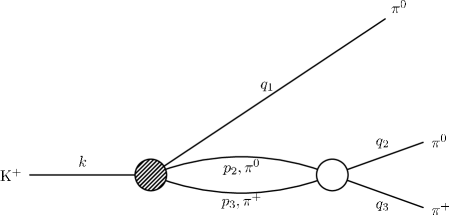
Figure 4: The $\pi^{+}\pi^{0}$ contribution.

Figure 4 shows the two-pion rescattering in one of the two $\pi^{+}\pi^{0}$ channels (the other is obtained by the exchange $q_{1}\leftrightarrow q_{2}$). Here the situation is simpler since there is only one possible intermediate state:

$$\begin{split}({\rm Im\,}\mathcal{M}_{00+})_{\pi^{0}\pi^{+}}=\frac{1}{2}\int&\frac{d^{3}p_{2}d^{3}p_{3}}{4E_{2}E_{3}}\delta^{4}(p_{2}+p_{3}-q_{2}-q_{3})\,{\rm Re\,}\mathcal{M}_{+0}\left((q_{2}+q_{3})^{2}\right)\\ &\quad\quad\quad\quad{\rm Re\,}\mathcal{M}_{00+}\left((q_{2}+q_{3})^{2},(q_{1}+p_{3})^{2},(q_{1}+p_{2})^{2}\right)\\ &+(q_{1}\leftrightarrow q_{2})\end{split}$$ (90)

As anticipated, to a good approximation we can neglect the quadratic terms in eq. (74). In this limit we obtain

$$({\rm Im\,}A_{00+})_{\pi^{0}\pi^{+}} = ({\rm Im\,}A^{(1)}_{00+})_{\pi^{0}\pi^{+}}+({\rm Im\,}A^{(2)}_{00+})_{\pi^{0}\pi^{+}}$$ (91)

$$\equiv ({\rm Im\,}A^{(1)}_{00+})_{\pi^{0}\pi^{+}}~{}+~{}(s_{1}\leftrightarrow s_{2})$$

with

$$({\rm Im\,}A^{(1)}_{00+})_{\pi^{0}\pi^{+}}=2a_{+0}(s_{1})v_{+0}(s_{1})R^{0}\left(\langle s\rangle_{1}-\Delta_{1}\right)+a_{1}v^{3}_{+0}(s_{1})A^{0}g^{0}~{}\frac{s_{1}(s_{3}-s_{2})}{16m^{4}_{\pi^{+}}}~{},$$ (92)

where the “velocity” $v_{+0}(s)$ and $\Delta_{i}$ are defined by

$$v_{+0}(s) = \frac{\left(s-(m_{\pi^{+}}+m_{\pi^{0}})^{2}\right)^{1/2}\left(s-(m_{\pi^{+}}-m_{\pi^{0}})^{2}\right)^{1/2}}{s}$$ (93)

$$\Delta_{i} = \frac{(m_{\pi^{+}}^{2}-m_{\pi^{0}}^{2})(m_{K}^{2}-m_{\pi^{0}}^{2})}{4s_{i}}$$ (94)

Finally, we must take into account the effective $3\pi\to 3\pi$ scattering due to reducible diagrams of the type in fig. 1c. By construction, these contributions are at least of $O(a_{i}^{2})$ and at this level of accuracy contribute only to the real part of the amplitude. Following the decomposition in eq. (69)–(70), the various rescattering combinations of the type in fig. 1c can be divided into two main groups: those which can be reabsorbed into a redefinition of ${\rm Re\,}A_{00+}$ and those which affect ${\rm Re\,}B_{00+}$. We shall start from the latter, that are more relevant for the structure of the cusp.

The $O(a_{i}^{2})$ corrections to ${\rm Re\,}B_{00+}$ arise from diagrams of the type in fig. 1c with the identification $\{\pi_{a},\pi_{b},\pi_{c}\}\equiv\{\pi^{+},\pi^{0},\pi^{0}\}$ and $\{\pi^{\prime\prime}_{b},\pi^{\prime}_{c}\}\equiv\{\pi^{\pm}\pi^{\mp}\}$. We can express all these contributions as

$$({\rm Re\,}B_{00+})_{{\rm fig}.\,\ref{fig:3p}c} = -2a_{x}(s_{3})\times\left[({\rm Im\,}C_{++-})_{\pi^{+}\pi^{+}\,}(\langle s\rangle_{3})\right.$$ (95)

$$\left.+({\rm Im\,}C^{(1)}_{++-})_{\pi^{+}\pi^{-}\,}(\langle s\rangle_{3})+v_{00}(\langle s\rangle_{3})({\rm Im\,}D^{(1)}_{++-})_{\pi^{0}\pi^{0}\,}(\langle s\rangle_{3})\right]$$

As we shall see in the next section, the three terms in the r.h.s. of eq. (95) correspond to the cases where the $\{\pi^{\prime}_{a},\pi^{\prime}_{b}\}$ pair is identified with $\{\pi^{+},\pi^{+}\}$, $\{\pi^{+},\pi^{-}\}$, or $\{\pi^{0},\pi^{0}\}$. Summing these three terms we find

$$({\rm Re\,}B_{00+})_{{\rm fig}.\,\ref{fig:3p}c} = -2a_{x}(s_{3})\left[a_{++}(\langle s\rangle_{3})v_{\pm}(\langle s\rangle_{3})R^{+}(\langle s\rangle_{3})\right.$$

$$\left.+2a_{+-}(\langle s\rangle_{3})v_{\pm}(\langle s\rangle_{3})R^{+}(\langle\langle s\rangle\rangle_{3})+a_{x}(\langle s\rangle_{3})v_{00}(\langle s\rangle_{3})R^{0}(\langle s\rangle_{3})\right]$$

where $\langle\langle s\rangle\rangle_{3}=(3s_{0}+s_{3})/4$ and, given we are already at $O(a_{i}^{2})$, we have neglected the tiny P-wave contribution and the difference between $s_{0}^{0}$ and $s_{0}^{+}$ in the $\langle s\rangle_{i}$ variables.

Far from the Dalitz plot boundaries, the $O(a_{i}^{2})$ corrections to ${\rm Re\,}A_{00+}$ could be ignored since they can be reabsorbed into a redefinition of $R^{0}(s)$. However, the polynomial form of $R^{0}(s)$ is not appropriate to describe the square-root singularities that occur at the borders of the Dalitz plot and, particularly, at $\pi^{0}\pi^{0}$ and $\pi^{+}\pi^{0}$ thresholds. The latter are described at $O(a_{i}^{2})$ accuracy by the remaining diagrams of the type in fig. 1c. The singularities at the $\pi^{0}\pi^{0}$ threshold, that are obtained with the identification $\{\pi^{\prime\prime}_{b},\pi^{\prime}_{c}\}\equiv\{\pi^{0}\pi^{0}\}$, are

$$(\delta{\rm Re\,}A_{00+})_{{\rm fig}.~{}\ref{fig:3p}c}^{\pi^{0}\pi^{0}} = -a_{00}(s_{3})v_{00}(s_{3})\times\left[({\rm Im\,}A^{(1)}_{+00})_{\pi^{+}\pi^{0}\,}(\langle s\rangle_{3})+({\rm Im\,}A^{(2)}_{+00})_{\pi^{+}\pi^{0}\,}(\langle s\rangle_{3})\right]$$ (97)

$$=-4a_{00}(s_{3})v_{00}(s_{3})a_{+0}(\langle s\rangle_{3})v_{+0}(\langle s\rangle_{3})R^{0}(\langle\langle s\rangle\rangle_{3})$$

where again we have neglected the tiny P-wave contribution and the difference between $\pi^{0}$ and $\pi^{+}$ masses in the $\langle s\rangle_{i}$ variables. The singularities at the $\pi^{+}\pi^{0}$ thresholds, obtained with $\{\pi^{\prime\prime}_{b},\pi^{\prime}_{c}\}\equiv\{\pi^{+}\pi^{0}\}$ or $\{\pi^{0}\pi^{+}\}$, are

$$(\delta{\rm Re\,}A_{00+})_{{\rm fig}.~{}\ref{fig:3p}c}^{\pi^{+}\pi^{0}} = -2a_{+0}(s_{1})v_{+0}(s_{1})\times\left[({\rm Im\,}A^{(2)}_{+00})_{\pi^{+}\pi^{0}\,}(\langle s\rangle_{1})+({\rm Im\,}A_{+00})_{\pi^{0}\pi^{0}\,}(\langle s\rangle_{1})\right.$$ (98)

$$\left.+v_{\pm}(\langle s\rangle_{1})({\rm Im\,}B_{+00})_{\pi^{+}\pi^{-}\,}(\langle s\rangle_{1})\right]~{}+~{}(s_{1}\leftrightarrow s_{2})$$

$$= -2a_{+0}(s_{1})v_{+0}(s_{1})\left[2a_{+0}(\langle s\rangle_{1})v_{+0}(\langle s\rangle_{1})R^{0}(\langle\langle s\rangle\rangle_{1})\right.$$

$$\left.+a_{00}(\langle s\rangle_{1})v_{00}(\langle s\rangle_{1})R^{0}(\langle s\rangle_{1})+2a_{x}(\langle s\rangle_{1})v_{+-}(\langle s\rangle_{1})R^{+}(\langle s\rangle_{1})\right]$$

$$~{}+~{}(s_{1}\leftrightarrow s_{2})$$

In summary, the relevant contribution to the $K^{+}\rightarrow\pi^{+}\pi^{0}\pi^{0}\,$ amplitude (in addition to ${\rm Re\,}A_{00+}$) are:

$${\rm Im\,}B_{00+} = 2a_{x}(s_{3})R^{+}(\langle s\rangle_{3}),$$ (99)

$${\rm Re\,}B_{00+} = -2a_{x}(s_{3})\left[a_{x}(s_{3})v_{00}(s_{3})R^{0}(s_{3})+a_{00}(s_{3})v_{00}(s_{3})R^{+}(\langle s\rangle_{3})\right.$$ (100)

$$\left.+a_{++}(\langle s\rangle_{3})v_{\pm}(\langle s\rangle_{3})R^{+}(\langle s\rangle_{3})+2a_{+-}(\langle s\rangle_{3})v_{\pm}(\langle s\rangle_{3})R^{+}(\langle\langle s\rangle\rangle_{3})\right.$$

$$\left.+a_{x}(\langle s\rangle_{3})v_{00}(\langle s\rangle_{3})R^{0}(\langle s\rangle_{3})\right]$$

$${\rm Im\,}A_{00+} = a_{00}(s_{3})v_{00}(s_{3})R^{0}(s_{3})+\Big{[}2a_{+0}(s_{1})v_{+0}(s_{1})R^{0}\left(\langle s\rangle_{1}-\Delta_{1}\right)$$ (101)

$$\qquad+a_{1}v^{3}_{+0}(s_{1})A^{0}g^{0}~{}\frac{s_{1}(s_{3}-s_{2})}{16m^{4}_{\pi^{+}}}~{}+~{}(s_{1}\leftrightarrow s_{2})\Big{]}$$

In order to take into account also the $O(a_{i}^{2})$ singularities at the Dalitz-plot boundaries, ${\rm Re\,}A_{00+}$ must be modified with the addition of the following extra term:

$${\rm Re\,}A_{00+}\to R^{0}(s_{3})+\delta{\rm Re\,}A_{00+}$$ (102)

$$\delta{\rm Re\,}A_{00+} = -4a_{00}(s_{3})v_{00}(s_{3})a_{+0}(\langle s\rangle_{3})v_{+0}(\langle s\rangle_{3})$$ (103)

$$-\Big{\{}2a_{+0}(s_{1})v_{+0}(s_{1})\big{[}2a_{+0}(\langle s\rangle_{1})v_{+0}(\langle s\rangle_{1})R^{0}(\langle\langle s\rangle\rangle_{1})$$

$$\qquad+a_{00}(\langle s\rangle_{1})v_{00}(\langle s\rangle_{1})R^{0}(\langle s\rangle_{1})$$

$$\qquad+2a_{x}(\langle s\rangle_{1})v_{+-}(\langle s\rangle_{1})R^{+}(\langle s\rangle_{1})\big{]}~{}+~{}(s_{1}\leftrightarrow s_{2})\Big{\}}$$

4.3 Rescattering in $K^{+}\rightarrow\pi^{+}\pi^{+}\pi^{-}\,$

In evaluating the coefficient of the cusp for the $K^{+}\rightarrow\pi^{+}\pi^{0}\pi^{0}\,$ decay we need to extract from data the real part of the $K^{+}\rightarrow\pi^{+}\pi^{+}\pi^{-}\,$amplitude. We thus need a suitable parameterization of the latter at the same level of accuracy. Since in the $K^{+}\rightarrow\pi^{+}\pi^{+}\pi^{-}\,$case the physical region is always above threshold, we do not expect any correction at $O(a_{i})$ in the decay distribution. This implies that the parametrization (75) for ${\rm Re\,}C_{++-}$ determines the real part of the $K^{+}\rightarrow\pi^{+}\pi^{+}\pi^{-}\,$decay amplitude at $O(a_{i})$ accuracy. Since the $K^{+}\rightarrow\pi^{+}\pi^{+}\pi^{-}\,$amplitude appears only multiplied by $O(a_{i})$ coefficients in the $K^{+}\rightarrow\pi^{+}\pi^{0}\pi^{0}\,$ rate, knowing the $K^{+}\rightarrow\pi^{+}\pi^{+}\pi^{-}\,$amplitude at $O(a_{i})$ accuracy is sufficient to the purpose of evaluating the cusp effect in $K^{+}\rightarrow\pi^{+}\pi^{0}\pi^{0}\,$ at the $O(a^{2}_{i})$ level.

However, it is worth to stress that the $O(a^{2}_{i})$ corrections to the $K^{+}\rightarrow\pi^{+}\pi^{+}\pi^{-}\,$decay amplitude have their own interest: at the border of the Dalitz plot they give rise to square-root singularities that could eventually be detected. Their inclusion would therefore improve the quality of the $K^{+}\rightarrow\pi^{+}\pi^{+}\pi^{-}\,$parameterization and could even be used to extract an additional information about the $\pi\pi\,$re-scattering. For this reason, in the following we shall provide a complete parameterization of the re-scattering effects in the $K^{+}\rightarrow\pi^{+}\pi^{+}\pi^{-}\,$amplitude to $O(a^{2}_{i})$ accuracy.

We start from the expression in eq. (71) and the parametrization (75), where the notation of the momenta is defined by

$$K^{+}\to\pi^{+}(q_{1})+\pi^{+}(q_{2})+\pi^{-}(q_{3});\quad\quad s_{1}=(q_{2}+q_{3})^{2},\text{ etc.}$$

In analogy with the $K^{+}\rightarrow\pi^{+}\pi^{0}\pi^{0}\,$ case, we decompose the amplitude isolating explicitly the cusp effect related to the $\pi^{0}\pi^{0}\leftrightarrow\pi^{+}\pi^{-}$ transition. In the physical case, where $m_{\pi^{+}}>m_{\pi^{0}}$, this cusp effect is not observable; however, the corresponding amplitude is still well defined. As discussed in section 3.3, this cusp amplitude is more conveniently analysed in the unphysical scenario with $m_{\pi^{0}}>m_{\pi^{+}}$. In this scenario the $\pi^{0}\pi^{0}\,$ threshold gives rise to two square-root singularities, respectively in $s_{1}$ and in $s_{2}$. To cover the case where either $s_{1}$ or $s_{2}$ are below the respective threshold, eq. (71) must be completed as follows:

$$\mathcal{M}_{++-} =C_{++-}+D^{(1)}_{++-}v_{00}(s_{1})+D^{(2)}_{++-}v_{00}(s_{2}) s_{1,2}>4m_{\pi^{0}}^{2},$$ (104)

$$\mathcal{M}_{++-} =C_{++-}+iD^{(1)}_{++-}v_{00}(s_{1})+D^{(2)}_{++-}v_{00}(s_{2}) s_{1}<4m_{\pi^{0}}^{2},$$ (105)

$$\mathcal{M}_{++-} =C_{++-}+D^{(1)}_{++-}v_{00}(s_{1})+iD^{(2)}_{++-}v_{00}(s_{2}) s_{2}<4m_{\pi^{0}}^{2}$$ (106)

We can choose $m_{\pi^{0}}$ close to $m_{\pi^{+}}$ so that $s_{1}$ and $s_{2}$ cannot simultaneously be below the $\pi^{0}\pi^{0}\,$ threshold.

As far as the two-pion scattering is concerned, we must take into account $\pi^{0}\pi^{0}\,$, $\pi^{+}\pi^{-}\,$and $\pi^{+}\pi^{+}\,$intermediate states. In computing the $\pi^{0}\pi^{0}\,$ contribution to $D^{(1)}_{++-}$ and $D^{(2)}_{++-}$ we will assume that ${\rm Re\,}A_{00+}$ is only a function of $s_{3}$ as in the parametrization (74), and obtain

$$({\rm Im\,}D^{(1,2)}_{++-})_{\pi^{0}\pi^{0}\,}=a_{x}(s_{1,2})R^{0}(s_{1,2})$$ (107)

Analogously, for the $\pi^{+}\pi^{+}\,$intermediate state we obtain

$$({\rm Im\,}C_{++-})_{\pi^{+}\pi^{+}\,}=a_{++}(s_{3})v_{\pm}(s_{3})R^{+}(s_{3})$$ (108)

We next consider the contribution of $\pi^{+}\pi^{-}\,$$\rightarrow\,$$\pi^{+}\pi^{-}\,$rescattering, whose general expression is.

$$\begin{split}({\rm Im\,}\mathcal{M}_{++-})_{\pi^{+}\pi^{-}\,}=\frac{1}{2}\int&\frac{d^{3}p_{2}d^{3}p_{3}}{4E_{2}E_{3}}\delta^{4}(p_{2}+p_{3}-q_{2}-q_{3})\,{\rm Re\,}\mathcal{M}_{+-}\left((q_{2}+q_{3})^{2}\right)\\ &\quad\quad\quad\quad{\rm Re\,}\mathcal{M}_{++-}\left((q_{2}+q_{3})^{2},(q_{1}+p_{3})^{2},(q_{1}+p_{2})^{2}\right)\\ &+(q_{1}\leftrightarrow q_{2})\end{split}$$ (109)

Above either of the $\pi^{0}\pi^{0}\,$ thresholds in $s_{1}$ and $s_{2}$, we can neglect the contributions of the real parts of $D^{1,2}_{++-}$ to ${\rm Re\,}\mathcal{M}_{++-}$ that, as we will shortly see, are $O(a_{i}^{2})$ and give a $O(a_{i}^{3})$ contribution to (109). Using the parametrization (75) and considering only S-wave scattering leads to

$$({\rm Im\,}C_{++-})_{\pi^{+}\pi^{-}\,}=({\rm Im\,}C^{(1)}_{++-})_{\pi^{+}\pi^{-}\,}+({\rm Im\,}C^{(2)}_{++-})_{\pi^{+}\pi^{-}\,}$$ (110)

with

$$({\rm Im\,}C^{(1,2)}_{++-})_{\pi^{+}\pi^{-}\,}=2a_{+-}(s_{1,2})v_{\pm}(s_{1,2})R^{+}(\langle s\rangle_{1,2})$$ (111)

Note that, although for simplicity of notations we use the same symbol adopted in eq. (84), in the $K^{+}\rightarrow\pi^{+}\pi^{+}\pi^{-}\,$case the $\langle s\rangle_{i}$ variables are defined by

$$\langle s\rangle_{i}=\frac{3s^{0}_{+}-s_{i}}{2}$$ (112)

i.e. we must replace $s^{0}_{0}$ with $s^{0}_{+}$ with respect to eq. (84). If we take into account also the tiny P-wave contribution, the above result is modified as follows

$$({\rm Im\,}C^{(1)}_{++-})_{\pi^{+}\pi^{-}\,} = 2a_{+-}(s_{1})v_{\pm}(s_{1})R^{+}(\langle s\rangle_{1})\,+a_{1}v^{3}_{\pm}(s_{1})A^{+}g^{+}~{}\frac{s_{1}(s_{3}-s_{2})}{16m^{4}_{\pi^{+}}}$$ (113)

At this point we could consider the (unphysical) case where $s_{1}<4m_{\pi^{0}}^{2}$. Here using eq. (105) we see that the real part of $\mathcal{M}_{++-}$ also receives a contribution from the imaginary part of $D^{(1)}_{++-}$ that, when injected in (109) produces a contribution to the real part of $D^{(1)}_{++-}$. Another contribution to ${\rm Re\,}D^{(1)}_{++-}$ below the $\pi^{0}\pi^{0}\,$ threshold arises from the ${\rm Im\,}D_{\pm}$ term in ${\rm Re\,}\mathcal{M}_{+-}$, see eqs. (63) and (66). Both these contributions are $O(a_{i}^{2})$ and lead to

$$\begin{split}({\rm Re\,}D^{(1)}_{++-})_{\pi^{+}\pi^{-}\,}&=-\frac{4}{\pi}\int\frac{d^{3}p_{2}d^{3}p_{3}}{4E_{2}E_{3}}\delta^{4}(p_{2}+p_{3}-q_{2}-q_{3})\,\\ &\quad\quad\left(R^{+}((q_{1}+p_{2})^{2})a_{x}^{2}(s_{1})+R^{0}(s_{1})a_{x}(s_{1})a_{\pm}(s_{1})\right)\end{split}$$ (114)

$$=-2v_{\pm}(s_{1})\left[R^{+}(\langle s\rangle_{1})a_{x}^{2}(s_{1})+R^{0}(s_{1})a_{x}(s_{1})a_{\pm}(s_{1})\right]$$ (115)

Finally, we must take into account the effective $3\pi\to 3\pi$ scattering due to reducible diagrams of the type in fig. 1c. As in the $K^{+}\to\pi^{+}\pi^{0}\pi^{0}$ case, these contributions are of $O(a_{i}^{2})$ and contribute only to the real part of the amplitude. The $O(a_{i}^{2})$ corrections to $D^{(1,2)}_{++-}$ are

$$({\rm Re\,}D^{(1)}_{++-})_{{\rm fig}.~{}\ref{fig:3p}c} = -a_{x}(s_{1})\times\left[({\rm Im\,}A^{(1)}_{00+})_{\pi^{0}\pi^{+}}(\langle s\rangle_{1})+({\rm Im\,}A^{(2)}_{00+})_{\pi^{0}\pi^{+}}(\langle s\rangle_{1})\right]$$ (116)

$$= -4a_{x}(s_{1})a_{+0}(\langle s\rangle_{1})v_{+0}(\langle s\rangle_{1})R^{0}\left(\langle\langle s\rangle\rangle_{1}\right)$$

While the remaining $O(a_{i}^{2})$ corrections, that can be absorbed into a redefinition of the ${\rm Re\,}C_{++-}$, are

$$(\delta{\rm Re\,}C_{++-})_{{\rm fig}.~{}\ref{fig:3p}c}^{\pi^{+}\pi^{+}} = -a_{++}(s_{3})v_{\pm}(s_{3})\times\left[({\rm Im\,}C^{(1)}_{++-})_{\pi^{+}\pi^{-}\,}(\langle s\rangle_{3})+({\rm Im\,}C^{(2)}_{++-})_{\pi^{+}\pi^{-}\,}(\langle s\rangle_{3})\right.$$ (117)

$$\left.+v_{00}(\langle s\rangle_{3})({\rm Im\,}D^{(1)}_{++-})_{\pi^{0}\pi^{0}\,}(\langle s\rangle_{3})+v_{00}(\langle s\rangle_{3})({\rm Im\,}D^{(2)}_{++-})_{\pi^{0}\pi^{0}\,}(\langle s\rangle_{3})\right]$$

$$= -a_{++}(s_{3})v_{\pm}(s_{3})\left[2a_{x}(\langle s\rangle_{3})v_{00}(\langle s\rangle_{3})R^{0}(\langle s\rangle_{3})\right.$$

$$\left.+4a_{+-}(\langle s\rangle_{3})v_{\pm}(\langle s\rangle_{3})R^{+}(\langle\langle s\rangle\rangle_{3})\right]$$

and

$$(\delta{\rm Re\,}C_{++-})_{{\rm fig}.~{}\ref{fig:3p}c}^{\pi^{+}\pi^{-}} = -2a_{+-}(s_{1})v_{\pm}(s_{1})\times\left[({\rm Im\,}C_{++-})_{\pi^{+}\pi^{+}}(\langle s\rangle_{1})+({\rm Im\,}C^{(2)}_{++-})_{\pi^{+}\pi^{-}\,}(\langle s\rangle_{1})\right.$$ (118)

$$\left.+v_{00}(\langle s\rangle_{1})({\rm Im\,}D^{(2)}_{++-})_{\pi^{+}\pi^{-}\,}(\langle s\rangle_{1})\right]~{}+~{}(s_{1}\leftrightarrow s_{2})$$

$$= -2a_{+-}(s_{1})v_{+-}(s_{1})\left[2a_{+-}(\langle s\rangle_{1})v_{+-}(\langle s\rangle_{1})R^{+}(\langle s\rangle_{1})\right.$$

$$\left.+2a_{+-}(\langle s\rangle_{1})v_{+-}(\langle s\rangle_{1})R^{+}(\langle\langle s\rangle\rangle_{1})+a_{x}(\langle s\rangle_{1})v_{00}(\langle s\rangle_{1})R^{0}(\langle s\rangle_{1})\right]$$

$$~{}+~{}(s_{1}\leftrightarrow s_{2})$$

In summary, the relevant contributions to the $K^{+}\rightarrow\pi^{+}\pi^{+}\pi^{-}\,$amplitude (in addition to ${\rm Re\,}C_{++-}$) are:

$${\rm Im\,}D^{(1)}_{++-} = a_{x}(s_{1})R^{0}(s_{1}),$$ (119)

$${\rm Re\,}D^{(1)}_{++-} = -2a_{x}(s_{1})\left[v_{\pm}(s_{1})R^{+}(\langle s\rangle_{1})a_{x}(s_{1})+v_{\pm}(s_{1})R^{0}(s_{1})a_{\pm}(s_{1})\right.$$ (120)

$$\left.+2v_{+0}(\langle s\rangle_{1})a_{+0}(\langle s\rangle_{1})R^{0}\left(\langle\langle s\rangle\rangle_{1}\right)\right]$$

$${\rm Im\,}C_{++-} = a_{++}(s_{3})v_{\pm}(s_{3})R^{+}(s_{3})+\Big{[}2a_{+-}(s_{1})v_{\pm}(s_{1})R^{+}(\langle s\rangle_{1})$$ (121)

$$+a_{1}v^{3}_{\pm}(s_{1})A^{+}g^{+}~{}\frac{s_{1}(s_{3}-s_{2})}{16m^{4}_{\pi^{+}}}+~{}(s_{1}\leftrightarrow s_{2})\Big{]}$$

4.4 The $K_{L}\to 3\pi$ system

The two $K_{L}\to 3\pi$ coupled channels form a system very similar to the one of the two $K^{+}\to 3\pi$ decays. Similarly to the charged modes, we can decompose the two $K_{L}$ decay amplitudes into regular terms and terms that are singular at the $\pi^{+}\pi^{-}\,$($\pi^{0}\pi^{0}\,$) threshold:

$$\mathcal{M}_{000} = A_{000}+\sum_{i=1\ldots 3}B^{(i)}_{000}v_{\pm}(s_{i})\left[\Theta(s_{i}-4m_{\pi^{+}}^{2})+i\Theta(4m_{\pi^{+}}^{2}-s_{i})\right]~{},$$ (122)

$$\mathcal{M}_{+-0} = C_{+-0}+D_{++0}v_{00}(s_{3})\left[\Theta(s_{3}-4m_{\pi^{0}}^{2})+i\Theta(4m_{\pi^{3}}^{2}-s_{i})\right]~{}.$$ (123)

Concerning the leading amplitudes (${\rm Re\,}A_{000}$ and ${\rm Re\,}C_{+-0}$) we shall adopt the following phenomenological parametrization:

$${\rm Re\,}A_{000}(s_{1},s_{2},s_{3}) =R_{L}^{0}(s_{1},s_{2},s_{3})=A_{L}^{0}\left[1+\tilde{h}_{L}^{0}\sum_{i=1\ldots 3}(s_{i}-s^{0}_{0_{L}})^{2}/3m_{\pi^{+}}^{4}\right]$$ (124)

$${\rm Re\,}C_{+-0}(s_{1},s_{2},s_{3}) =R_{L}^{+}\!(s_{3})=A_{L}^{+}\left[1+g_{L}^{+}\!(s_{3}-s^{+}_{0_{L}})/2m_{\pi^{+}}^{2}+\tilde{h}_{L}^{+}\!(s_{3}-s^{+}_{0_{L}})^{2}/2m_{\pi^{+}}^{4}\right]$$ (125)

where

$$\sum_{i=1\ldots 3}s_{i}=\left\{\begin{array}[]{ll}3s_{0_{L}}^{0}=m_{K}^{2}+3m^{2}_{\pi^{0}}&(K_{L}\to 3\pi^{0})\\ 3s_{0_{L}}^{+}=m_{K}^{2}+2m^{2}_{\pi^{+}}+m_{\pi^{0}}&(K_{L}\to\pi^{+}\pi^{-}\pi^{0})\end{array}\right.$$ (126)

The values of the $K_{L}\to\pi^{+}\pi^{-}\pi^{0}$ slopes fitted by PDG (that also includes a small term proportional to $(s_{1}-s_{2})^{2}$) are $g_{L}^{+}\approx 0.678\pm 0.008$ and $\tilde{h}_{L}^{+}\approx h_{\text{\tiny PDG}}-(g_{L}^{+}/2)^{2}=0.04\pm 0.01$. In the $K_{L}\to 3\pi^{0}$ case the linear term is forbidden by Bose symmetry; the normalization of the quadratic term has been chosen such that $\tilde{h}_{L}^{0}\approx h_{\text{\tiny PDG}}\approx-(5.0\pm 1.4)\times 10^{-3}$.

Here the visible cusp due to the $\pi^{+}\pi^{-}\to\pi^{0}\pi^{0}$ rescattering is expected in the $K_{L}\to 3\pi^{0}$ spectrum. The phenomenon is completely analog to what happens in the charged modes; however, the relative size of the cusp is smaller because of the inverted hierarchy in the leading amplitudes: in the isospin limit $A_{L}^{+}/A_{L}^{0}=1/3$, to be compared with the analogous ratio $A^{+}/A^{0}=2$ of the charged modes.

The calculation of the imaginary parts of the amplitudes (and the real part of the cusp coefficient) proceeds exactly as in the charged modes. We report here only the results. In the interesting case of the $K_{L}\to 3\pi^{0}$ amplitude, the imaginary parts are

$$({\rm Im\,}B^{(i)}_{000})_{\pi^{+}\pi^{-}\,} = 2a_{x}(s_{i})R_{L}^{+}(s_{i})~{},$$ (127)

$$({\rm Im\,}A_{000})_{\pi^{0}\pi^{0}\,} = \sum_{i=1\ldots 3}a_{00}(s_{i})v_{00}(s_{i})R_{L}^{0}(s_{i},\langle s\rangle_{i},\langle s\rangle_{i})~{},$$ (128)

with

$$\langle s\rangle_{i}=\frac{3s^{0}_{0_{L}}-s_{i}}{2}~{},$$ (129)

while the $O(a_{i}^{2})$ corrections to the (visible) cusp amplitude are

$$({\rm Re\,}B^{(i)}_{000})_{{\rm fig}.~{}\ref{fig:3p}a} = -2v_{00}(s_{i})a_{x}(s_{i})\left[a_{x}(s_{i})R_{L}^{0}(s_{i},\langle s\rangle_{i},\langle s\rangle_{i})+a_{00}(s_{i})R^{+}(s_{i})\right]~{},$$ (130)

$$({\rm Re\,}B^{(i)}_{000})_{{\rm fig}.~{}\ref{fig:3p}c} = -8a_{x}(s_{i})a_{+0}(\langle s\rangle_{i})v_{+0}(\langle s\rangle_{i})R^{+}(\langle\langle s\rangle\rangle_{i})~{}.$$ (131)

For the auxiliary mode, $K_{L}\to\pi^{+}\pi^{-}\pi^{0}$, we find

$$({\rm Im\,}D_{+-0})_{\pi^{0}\pi^{0}\,} = a_{x}(s_{3})R_{L}^{0}(s_{3},\langle s\rangle_{3},\langle s\rangle_{3})~{},$$ (132)

$$({\rm Im\,}C_{+-0})_{\pi^{\pm}\pi^{0}} = 2a_{+0}(s_{1})v_{+0}(s_{1})R_{L}^{+}\left(\langle s\rangle_{1}+\Delta_{1_{L}}\right)$$ (133)

$$+ a_{1}v^{3}_{+0}(s_{1})A_{L}^{+}g_{L}^{+}~{}\frac{s_{1}(s_{3}-s_{2})}{16m^{4}_{\pi^{+}}}~{}+~{}(s_{1}\leftrightarrow s_{2})~{},$$

with

$$\Delta_{i_{L}}=\frac{(m_{\pi^{+}}^{2}-m_{\pi^{0}}^{2})(m_{K}^{2}-m_{\pi^{+}}^{2})}{4s_{i}}$$ (134)

4.5 Decay rates and extraction of the scattering lengths

The aim of this paper is eminently practical. Our goal is

• to establish a parametrization of $K\to 3\pi$ amplitudes suitable to fit the experimental decay distributions at the 10^-3 level;

• describe the cusp effect due to the $\pi^{+}\pi^{-}\,\to\pi^{0}\pi^{0}\,$ rescattering with a theoretical error of a few %.

Since the cusp effect on the rate is $\sim 10\%$, the two requests are compatible. In this section we shall outline the basic strategy for the extraction of the combination of scattering lengths $a_{x}$, as defined in section 2.3, from a fit to the $K^{+}\rightarrow\pi^{+}\pi^{0}\pi^{0}\,$ decay distribution.

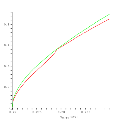
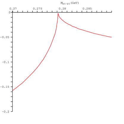
Figure 5: Illustration of the cusp effects in $K^{+}\rightarrow\pi^{+}\pi^{0}\pi^{0}\,$. Upper plot: differential decay distribution (in arbitrary units, as a function of the $\pi^{0}\pi^{0}$ invariant mass) with and without the cusp amplitude. Lower plot: relative size of the cusp amplitude with respect to the regular term. All plots have been obtained using the values of the scattering lengths and their effective ranges from Ref. [4] (see sect. 2.3).

From eqs. (69)–(70) the differential decay rate for $K^{+}\rightarrow\pi^{+}\pi^{0}\pi^{0}\,$ is

$$|\mathcal{M}_{00+}|^{2} =\left({\rm Re\,}A_{00+}+{\rm Re\,}B_{00+}v_{\pm}(s_{3})\right)^{2}+\left({\rm Im\,}A_{00+}+{\rm Im\,}B_{00+}v_{\pm}(s_{3})\right)^{2} s_{3}>4m_{\pi^{+}}^{2}$$

$$|\mathcal{M}_{00+}|^{2} =\left({\rm Re\,}A_{00+}-{\rm Im\,}B_{00+}v_{\pm}(s_{3})\right)^{2}+\left({\rm Im\,}A_{00+}+{\rm Re\,}B_{00+}v_{\pm}(s_{3})\right)^{2} s_{3}<4m_{\pi^{+}}^{2}$$

Expanding the various terms up to $O(a_{i}^{2})$, we can write

$$|\mathcal{M}_{00+}|^{2}=({\rm Re\,}A_{00+})^{2}+\Delta_{A}+v_{\pm}(s_{3})\Delta_{\rm cusp}+O(a_{i}^{3})$$ (135)

where

$$\Delta_{A} = ({\rm Im\,}A_{00+})^{2}+v^{2}_{\pm}(s_{3})({\rm Im\,}B_{00+})^{2}$$ (136)

$$\Delta_{\rm cusp} = \left\{\begin{array}[]{ll}-2{\rm Re\,}A_{00+}{\rm Im\,}B_{00+}&s_{3}<4m_{\pi^{+}}^{2}\\ 2{\rm Re\,}A_{00+}{\rm Re\,}B_{00+}+2{\rm Im\,}A_{00+}{\rm Im\,}B_{00+}&s_{3}>4m_{\pi^{+}}^{2}\end{array}\right.$$ (139)

The explicit expressions for the various terms are given in eqs. (99)–(101). At the same level of accuracy, the $K^{+}\rightarrow\pi^{+}\pi^{+}\pi^{-}\,$decay distribution in the physical region is

$$|\mathcal{M}_{++-}|^{2}=({\rm Re\,}C_{++-})^{2}+\Delta_{C}+O(a_{i}^{3})$$ (140)

with the $O(a_{i}^{2})$ correction given by

$$\Delta_{C} = \left[{\rm Im\,}C_{++-}+v_{00}(s_{1}){\rm Im\,}D^{(1)}_{++-}+v_{00}(s_{2}){\rm Im\,}D^{(2)}_{++-}\right]^{2}$$ (141)

$$+ 2{\rm Re\,}C_{++-}\left[v_{00}(s_{1}){\rm Re\,}D^{(1)}_{++-}+v_{00}(s_{2}){\rm Re\,}D^{(2)}_{++-}\right]$$

and the explicit expressions for the various terms reported in eqs. (119)–(121).

The cusp amplitude in eq. (139) contains both a leading $O(a_{i})$ term responsible for the negative square-root behavior of the rate below the threshold and an $O(a^{2}_{i})$ term that leads to a similar (smaller) behavior also above the threshold (see figure 5). Both these effects are proportional to $a_{x}$.

The precision with which the coupling $a_{x}$ can be extracted from data depends on the accuracy of our parametrization of the amplitudes and, in particular, on the theoretical expression for $\Delta_{\rm cusp}$. Since we have neglected $O(a_{i}^{3})$ terms, a priori we should expect relative corrections of $O(a_{i}^{2})$ to the value of $a_{x}$. Given the expected value of the scattering lengths and the effect of the $O(a^{2}_{i})$ terms in figure 5, a natural estimate of this error is about $5\%$. A posteriori checks about the size of this error can be obtained by studying the stability of the central value of $a_{x}$ obtained by means of different fitting procedures. In particular, it would be interesting to compare the results obtained under the following assumptions:

1. All the $a_{i}$ are treated as free parameters.

2. All the $a_{i}$ but $a_{x}$ are fixed to their standard values and only $a_{x}$ is treated as a free parameter.

3. The fit is extended up to the border of the Dalitz Plot with the inclusion of the $\delta{\rm Re\,}A_{00+}$ term in (103).

4. The expressions of $R^{+,0}(s)$ are modified with the inclusion of cubic terms in $(s_{3}-s_{0})$ and/or quadratic terms in $(s_{1}-s_{2})$.

5. One of the two $\Delta_{A,C}$ terms (or both) is ignored [in this way the regular amplitudes are re-defined by corrections of $O(a_{i}^{2})$; this, in turn, implies an $O(a_{i}^{2})$ effect on the extraction of $a_{x}$, of the same order of the terms which have not been computed].

Finally, it would certainly be quite useful to compare the value of $a_{x}$ extracted from $K^{+}\to 3\pi$ decays vs. the value extracted in a similar way from $K_{L}\to 3\pi$ decays.

5 Conclusions

We have outlined a method that allows to systematically evaluate rescattering effects in $K\to 3\pi$ decays by means of an expansion in powers of the $\pi\pi$ scattering lengths. This approach is less ambitious than the ordinary loop expansion performed in effective field theories, such as CHPT: the scope is not a dynamical calculation of the entire decay amplitudes, but a systematical evaluation of the singular terms due to rescattering effects only. In particular, our main goal has been a systematical description of the cusp effect in $K^{+}\rightarrow\pi^{+}\pi^{0}\pi^{0}\,$ [1] in terms of the $\pi\pi$ scattering lengths. From this point of view, the approach we have proposed is more efficient and substantially simpler than the ordinary perturbative expansion of CHPT.

Using this method we have explicitly computed all the $O(a_{i}^{2})$ corrections to the leading cusp effect in $K^{+}\rightarrow\pi^{+}\pi^{0}\pi^{0}\,$, extending the results of Ref. [1]. As shown in figure 5, these extra terms produce a small square-root behavior also above the $\pi^{+}\pi^{-}\,$singularity.

The present work allows to reduce the theoretical error on the extraction of $a_{0}-a_{2}$ from an experimental analysis of the $K^{+}\rightarrow\pi^{+}\pi^{0}\pi^{0}\,$ spectrum to about 5%. A similar level of theoretical accuracy is also achieved in the case of the $K_{L}\to 3\pi^{0}$ spectrum. This level of precision is probably not sufficient to fully exploit the potentially very accurate data of NA48, and is also quite above the error on the predictions of $a_{0}-a_{2}$ in Ref. [4]. To reach this level of precision, a complete evaluation of the $O(a_{i}^{3})$ corrections and — at the same time — of the effects due to radiative corrections is needed.

References

- [1] N. Cabibbo, Phys. Rev. Lett. 93 (2004) 121801.
- [2] Ulf-G. Meissner, G. Muller, and S. Steininger, Phys. Lett. B 406 (1997) 154.
- [3] S. Weinberg, Phys. Rev. Lett. 18 (1967) 188; Physica 96A (1979) 327; J. Gasser and H. Leutwyler, Ann. Phys. 158 (1984) 142; Nucl. Phys. B 250 (1985) 465.
- [4] G. Colangelo, J. Gasser and H. Leutwyler, Phys. Lett. B 488 (2000) 261 [hep-ph/0007112]; Nucl. Phys. B 603 (2001) 125.
- [5] S.M. Roy, Phys. Lett. B 36 (1971) 353.
- [6] B. Ananthanarayan, G. Colangelo, J. Gasser and H. Leutwyler, Phys. Rept. 353 (2001) 207. [hep-ph/0005297].
- [7] S. Pislak et al., Phys. Rev. D 67 (2003) 072004 [hep-ex/0301040]. For an independent analysis of the E865 data see: S. Descotes-Genon, N. H. Fuchs, L. Girlanda and J. Stern, Eur. Phys. J. C 24 (2002) 469 [hep-ph/0112088].
- [8] G. D’Ambrosio, G. Ecker, G. Isidori and H. Neufeld, Z. Phys. C 76 (1997) 301 [hep-ph/9612412]; A. Nehme, Phys. Rev. D 70 (2004) 094025 [hep-ph/0406209]; J. Bijnens and F. Borg, Eur. Phys. J. C 39 (2005) 347 [hep-ph/0410333]; hep-ph/0501163.
- [9] J. Kambor, J. Missimer and D. Wyler, Phys. Lett. B 261 (1991) 496; G. D’Ambrosio, G. Isidori, A. Pugliese and N. Paver, Phys. Rev. D 50 (1994) 5767 [hep-ph/9403235]; J. Bijnens, P. Dhonte and F. Borg, Nucl. Phys. B 648 (2003) 317 [hep-ph/0205341].
- [10] J. Bijnens and F. Borg, Nucl. Phys. B 697 (2004) 319 [hep-ph/0405025].
- [11] S. Weinberg, Phys. Rev. Lett. 4 (1960) 87.
- [12] G. Barton, C. Kacser, and S. P. Rosen. Phys. Rev. 130 (1963) 783.
- [13] J. A. Cronin. Phys. Rev. 161 (1967) 1483.
- [14] M. Knecht and R. Urech, Nucl. Phys. B 519 (1998) 329 [hep-ph/9709348].
- [15] J. Gasser, V. E. Lyubovitskij, A. Rusetsky and A. Gall, Phys. Rev. D 64 (2001) 016008 [hep-ph/0103157].
- [16] J. R. Pelaez and F. J. Yndurain, hep-ph/0412320.
- [17] E. H. Wichman and J. H. Crichton. Phys. Rev. 132 (1963) 2788.
- [18] J. R. Taylor. Phys. Rev. 142 (1966) 1236.
- [19] S. Weinberg, The Quantum Theory of Fields (Cambridge University Press, 1955).
- [20] S. Eidelman et al. [Review of Particle Physics], Phys. Lett. B 592 (2004) 1.