USTC-ICTS-05-03
Proton-Antiproton Annihilation in Baryonium

Abstract

A possible interpretation of the near-threshold enhancement in the $(p\bar{p})$-mass spectrum in $J/\psi{\to}\gamma p{\bar{p}}$ is the of existence of a narrow baryonium resonance $X(1860)$. Mesonic decays of the $(p\bar{p})$-bound state $X(1860)$ due to the nucleon-antinucleon annihilation are investigated in this paper. Mesonic coherent states with fixed $G$-parity and $P$-parity have been constructed . The Amado-Cannata-Dedoder-Locher-Shao formulation(Phys Rev Lett. 72, 970 (1994)) is extended to the decays of the $X(1860)$. By this method, the branch-fraction ratios of $Br(X\rightarrow\eta 4\pi)$, $Br(X\rightarrow\eta 2\pi)$ and $Br(X\rightarrow 3\eta)$ are calculated. It is shown that if the $X(1860)$ is a bound state of $(p\bar{p})$, the decay channel ($X\rightarrow\eta 4\pi)$ is favored over $(X\rightarrow\eta 2\pi)$. In this way, we develop criteria for distinguishing the baryonium interpretation for the near-threshold enhancement effects in $(p\bar{p})$-mass spectrum in $J/\psi{\to}\gamma p{\bar{p}}$ from other possibilities. Experimental checks are expected. An intuitive picture for our results is discussed.

I Introduction

There is growing interest in exotic hadrons, which may open new windows for understanding the hadronic structures and QCD at low energy. Recently, the BES Collaboration observed a near-threshold enhancement in the proton-antiproton $(p\bar{p})$ mass spectrum from the radiative decay $J/\psi\rightarrow\gamma p\bar{p}$ BES . This enhancement can be fitted with either an $S$- or $P$-wave Breit-Wigner resonance function. In the case of $S$-wave fit, the peak mass is at $M=1859_{-10}^{+3}({\rm stat})_{-25}^{+5}({\rm sys})$ with a total width $\Gamma<30~{}\mbox{MeV/c}^{2}$ at $90\%$ percent confidence level. For the $S-$wave fit, the corresponding spin and parity are $J^{PC}=0^{-+}$. Moreover, the Belle Collaboration also reported similar observations of the decays $B^{+}\rightarrow K^{+}p\bar{p}$ Bell1 and $\bar{B}^{0}\rightarrow D^{0}p\bar{p}$ Bell2 , showing enhancements in the $p\bar{p}$ invariant mass distributions near $2m_{p}$. These observations could be naively interpreted as signals for baryonium $p\bar{p}$ bound states Yang Datta Yan . The BES-datum fit in ref.BES represents the simplest interpretation of the experimental results as an indication of a baryonium resonance. Here, we denote this baryonium particle as $X(1860)$ with $J^{PC}=0^{-+}$ and $I^{G}=0^{+}$Peking . However, this is only one possible interpretation. Other possible ways to understand this phenomena include, for instance, a flavorless gluon stateRosner , a final state interactionsZou or an effect of the quark fragmentation processRosner , etc. In order to ascertain whether or not the $X(1860)$ exists, more evidence is needed. A significant distinguishing feature for the baryonium interpretation is that the decays of $X(1860)$ are mainly due to proton-antiproton annihilation in the baryonium. In this paper, we investigate $p\bar{p}$-annihilations in $X(1860)$ by means of a coherent-state method on nucleon-antinucleon annihilation in large $N_{c}$ QCDbatch1 batch2 .

At first glance, the most favorable $X(1860)$ decay channel would be $X(1860)\rightarrow\eta\pi\pi$, because it is the simplest hadronic process with the largest phase space. However, since the decay is caused by $(p\bar{p})$-annihilations in the $X(1860)$, this naive observation may be not true. Low-energy nucleon-antinucleon annihilation is a fertile area for studying low energy QCD, and there are many experimental and theoretical studies in the literature(e.g., see batch1 Yang lu3 batch2 Sedlak Amsler Sommermann Amado97 Amado94 ). In these reports, it has been shown that the nucleon-antinucleon annihilation at rest mostly favors processes with between 4 and 7 pion final states, over those with two or three pion’s Amado97 . This is a a general characteristic of $(p\bar{p})$-annihilation (without consideration of $J^{PC}$ and $I^{G}$ quantum numbers). It is interesting to pursue whether or not there are similar features in $X(1860)$ decay. If so, we will have a new criteria to characterize the $X(1860)$. This is the main aim of the work reported here.

The contents of this paper are organized as follows: In section II, we use a toy model to describe the possibility of the $(p-\bar{p})$-collisions inside a ($p\bar{p}$)-bound state; in section III, we construct the mesonic coherent states with fixed $G$- and $P$-parities; Section IV describes calculation of the branch fractions of $Br(X\rightarrow\eta 4\pi)$, $Br(X\rightarrow\eta 2\pi)$ and $Br(X\rightarrow 3\eta)$. Finally, we briefly summarize our results, and provide an intuitive picture for our results.

II A toy model description on $(p-\bar{p})$ collisions inside a ($p\bar{p}$)-bound state

In order to understand the mechanics of $X(1860)$ decays, we assume that the proton and the antiproton collide with each other inside the $X(1860)$, resulting in the collapse of the $(p\bar{p})$-bound state , or the decay due to the effect of rapid nucleon-antinucleon annihilation. We use the $(p-\bar{p})$-collision frequency $\nu$ (i.e., the collision times per time-unit period) in the $X(1860)$ to characterize the possibility of such $(p\bar{p})$-collisions. We show that this frequency can be estimated in a simple toy model, in which the proton and the antiproton are treated as point-like particles. This collision frequency is actually equivalent to the total $X(1860)$ decay width in the annihilation-assumption mentioned above. Following ref.Yan , we roughly sketch the toy model for the $X(1860)$ $(p\bar{p})$-bound state. The single-well potential toy model for the $(pn)$-molecular bound state deuteron first appeared in the literature more than fifty years ago Ma . The quasi-stable $(p\bar{p})$-molecular bound state $X(1860)$ can be similarly described by a double-well potential(or Skyrmion-type potential) toy modelDatta Yan . The potential of such a double-well model, $V(\rho)$, is expressed as followsYan (see Fig.1)

$$V(\rho)=2m_{p}-c\;\delta(\rho)+V_{c}(\rho),$$ (1)

where

$$V_{c}(\rho)=\left\{\begin{array}[]{ll}{h={m_{p}/4}},&0<\rho<\lambda,\\ -V_{p\bar{p}}=-73~{}\mbox{MeV},&\lambda<\rho<a_{p\bar{p}},\\ 0,&~{}~{}~{}~{}~{}\rho>a_{p\bar{p}}.\end{array}\right.$$ (2)

where $a_{p\bar{p}}\simeq 2~{}\mbox{fm}$, $c\simeq 2.161$ , $m_{p}$ is the mass of proton and $\lambda=1/(2m_{p})\simeq 0.1{\rm fm}$. In this case, the Schr${\rm\ddot{o}}$dinger equation for $S$-wave bound states is

$${-1\over 2(m_{p}/2)}{\partial^{2}\over\partial\rho^{2}}u(\rho)+\left[V(\rho)-E\right]u(\rho)=0,$$ (3)

where $u(\rho)=\rho\;\psi(\rho)$ is the radial wave function, and $m_{p}/2$ is the nucleon reduced mass. This equation can be solved analytically, and has a bound state $u_{2}(\rho)$ with binding energy $E_{2}\simeq-17.2~{}\mbox{MeV}$ due to the attractive square well potential at intermediate ranges (see Appendix). This molecular state is identified as the $X(1860)$.

Figure 1: The double well potential of $p\bar{p}$-system.

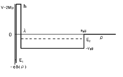
We use this solution to estimate the $(p\bar{p})$-collision frequency inside the $X(1860)$. Because of the effect of $(p\bar{p})$-annihilation, this bound state is not stable. Note that in this model, there are two attractive potential wells: one is at $\rho\sim 0$ and the other is at intermediate values; between them is a potential barrier. When $\rho\sim 0$, the proton and antiproton are in collision. Therefore, we can derive the $(p\bar{p})$-collision frequency in the inside of $X(1860)$ by calculating the quantum tunnelling effect for $u_{2}(\rho)$ passing through the potential barrier. In the WKB-approximation, the tunnelling coefficient (i.e., barrier penetrability) is (see Schiff’s book in ref.Ma )

$$T_{0} = \exp\left[-2\int_{0}^{\lambda}dr\sqrt{m_{p}(h-E_{2})}\right]$$ (4)

$$= \exp\left[-2\lambda\sqrt{m_{p}(h-E_{2})}\right].$$

For the region between $\rho=\lambda$ to $\rho=a_{p\bar{p}}$, the time-period $\theta$ for the particle’s round trip is

$$\theta={2\left[a_{p\bar{p}}-\lambda\right]\over v}=\left[a_{p\bar{p}}-\lambda\right]\sqrt{{m_{p}\over V_{p\bar{p}}+E_{2}}}.~{}$$ (5)

Thus, the state $X(1860)$’s (i.e.,$u_{2}(r)$) lifetime is $\tau=\theta T_{0}^{-1}$, and $\nu$, the the so called $p\bar{p}$-collision frequency inside the $X(1860)$, is equal to $\Gamma_{X}$, the total width of $X(1860)$:

$$\nu=\Gamma_{X}\equiv{1\over\tau}={1\over a_{p\bar{p}}-\lambda}\sqrt{{V_{p\bar{p}}+E_{2}\over m_{p}}}\exp\left[-2\lambda\sqrt{m_{p}(h-E_{2})}\right].~{}~{}$$

Substituting $E_{2}=-17.2~{}\mbox{MeV},\;a_{p\bar{p}}=2.0~{}\mbox{fm}$ into Eq.(II), we obtain the prediction

$$\Gamma_{X}\simeq 15.5~{}\mbox{MeV},$$ (6)

which is compatible with the experimental data BES .

The corresponding $(p\bar{p})$-collision frequency inside the $X(1860)$ is about

$$\nu=\Gamma_{X}/\hbar\simeq 2.35\times 10^{22}~{}~{}{\rm Hz}.$$ (7)

Note that because the binding energy $E_{2}$ is rather small (compared to $2m_{p}$), the annihilation processes that cause $X(1860)$ to be unstable occur nearly at rest.

III Coherent states with fixed $G-$ and $P-$parities

When the proton and antiproton collide, they will rapidly annihilate into mesons. The coherent state method in batch1 and batch2 investigates $(p\bar{p})$-annihilation at rest without consideration of the $P-$ and $G-$parity. In this paper we are concerned with annihilation inside the $X(1860)$ where the $(p\bar{p})$ state has $I^{G}(J^{PC})=0^{+}(0^{-+})$. For this state, the allowed processes are ($X(1860)\rightarrow\eta 2\pi;~{}~{}\eta 4\pi;\cdots\eta 2n\pi;~{}~{}3\eta$) (we ignore processes that involve K-mesons), where the $\pi$ and $\eta$ are both pseudoscalars and the $G$-parities are negative and positive respectively. In this case, we have to introduce $P-$ and $G-$parities into the previous coherent state description of mesons radiated in $(p\bar{p})$-annihilationsbatch1 ; batch2 .

We construct coherent states with fixed four momentum and fixed isospin, and, also, with fixed $G$ parity and $P$ parity. Following the method in batch1 batch2 , we first construct the field operator $F$ that creates a $\pi$ or $\eta$ at the space time point $x$ and directed in the isospin direction $\hat{\textbf{n}}$.

$$F(x,\hat{\textbf{n}})=\int d^{3}{\bf k}e^{-ik\cdot x}f(\textbf{k})\textbf{a}^{{\dagger}}_{\textbf{k}}\cdot\hat{\textbf{n}}+\int d^{3}{\bf q}e^{-iq\cdot x}g(\textbf{q})b^{{\dagger}}_{\textbf{q}},$$ (8)

where $k\cdot x=k_{0}t-\textbf{k}\cdot\textbf{x}$ with $k_{0}=\sqrt{\textbf{k}^{2}+m^{2}_{\pi}}$, $q\cdot x=q_{0}t-\textbf{q}\cdot\textbf{x}$ with $q_{0}=\sqrt{\textbf{q}^{2}+m^{2}_{\eta}}$, $\textbf{a}^{{\dagger}}_{\textbf{k}}$ is the isospin-triplet creation operator, and $b^{{\dagger}}_{\textbf{k}}$ is the isospin-singlet creation operator.  From the $G$- an $P$-parities of the $\pi$ and $\eta$, we have

$$\hat{G}{\bf{\pi}}(\textbf{x},t)\hat{G}^{{\dagger}} = -{\bf{\pi}}(\textbf{x},t)$$

$$\hat{G}\eta(\textbf{x},t)\hat{G}^{{\dagger}} = \eta(\textbf{x},t)$$

$$\hat{P}{\bf{\pi}}(\textbf{x},t)\hat{P}^{{\dagger}} = -{\bf{\pi}}(-\textbf{x},t)$$

$$\hat{P}\eta(\textbf{x},t)\hat{P}^{{\dagger}} = -\eta(-\textbf{x},t),$$ (9)

where $\hat{G}$, $\hat{P}$ are the unitary operators as follows

$$\hat{P} = \exp[i\frac{\pi}{2}\sum_{j,\textbf{k}}(a^{+}_{\textbf{k},j}a_{-\textbf{k},j}+b^{+}_{\textbf{k}}b_{-\textbf{k}}+a^{+}_{\textbf{k},j}a_{\textbf{k},j}+b^{+}_{\textbf{k}}b_{\textbf{k}})]$$

$$\hat{G} = \exp[i\frac{\pi}{2}\sum_{j,\textbf{k}}(a^{+}_{\textbf{k,-1}}a_{\textbf{k},1}+a^{+}_{\textbf{k,1}}a_{\textbf{k},-1}-a^{+}_{\textbf{k},1}a_{\textbf{k,1}}-a^{+}_{\textbf{k},-1}a_{\textbf{k,-1}})]\times$$ (10)

$$\exp[-\frac{\pi}{\sqrt{2}}\sum_{\textbf{k}}(a^{+}_{\textbf{k},0}a_{\textbf{k,1}}+a^{+}_{\textbf{k},0}a_{\textbf{k,-1}}-a^{+}_{\textbf{k},1}a_{\textbf{k},0}-a^{+}_{\textbf{k},-1}a_{\textbf{k},0})].$$

It is straight-forward to check the following equations

$$\hat{G}a^{{\dagger}}_{\textbf{p},i}\hat{G}^{{\dagger}} = -a^{{\dagger}}_{\textbf{p},i}$$

$$\hat{G}b^{{\dagger}}_{\textbf{q}}\hat{G}^{{\dagger}} = b^{{\dagger}}_{\textbf{q}}$$

$$\hat{P}a^{{\dagger}}_{\textbf{p},i}\hat{P}^{{\dagger}} = -a^{{\dagger}}_{-\textbf{p},i}$$

$$\hat{G}b^{{\dagger}}_{\textbf{q}}\hat{G}^{{\dagger}} = -b^{{\dagger}}_{-\textbf{q}}$$ (11)

where $i=1,0,-1$ corresponding to $\pi^{+},\pi^{0},\pi^{-}$. Under G transformation, $F(x,\hat{\textbf{n}})$ becomes

$$G(x,\hat{\textbf{n}})=\hat{G}F(x,\hat{\textbf{n}})\hat{G}^{{\dagger}}=-\int d^{3}{\bf k}f(\textbf{k})\textbf{a}^{{\dagger}}_{\textbf{k}}\cdot\hat{\textbf{n}}~{}~{}e^{-ik\cdot x}+\int d^{3}{\bf q}e^{-iq\cdot x}g(\textbf{q})b^{{\dagger}}_{\textbf{q}}.$$ (12)

For simplicity we take $f(-\textbf{k})=f(\textbf{k})$ and $g(-\textbf{q})=g(\textbf{q})$, then the P transformation of $F(x,\hat{\textbf{n}})$ is as follows

$$\hat{P}F(x,\hat{\textbf{n}})\hat{P}^{{\dagger}}=-\int d^{3}{\bf k}f(\textbf{k})\textbf{a}^{{\dagger}}_{\textbf{k}}\cdot\hat{\textbf{n}}~{}~{}e^{-ik\cdot x^{{}^{\prime}}}-\int d^{3}{\bf q}e^{-iq\cdot x^{{}^{\prime}}}g(\textbf{q})b^{{\dagger}}_{\textbf{q}}=-F(x^{{}^{\prime}},\hat{\textbf{n}}),$$ (13)

with $\textbf{x}^{{}^{\prime}}=(-\textbf{x},t)$. Then the desired coherent state with fixed four-momentum, fixed isospin, and also with well-defined G parity(+) and P parity(–) is constructed as follows

$$|K,I,I_{z}\rangle= \int\frac{d^{4}x}{(2\pi)^{4}}\frac{d\Omega_{\hat{\textbf{n}}}}{\sqrt{4\pi}}~{}e^{iK\cdot x}|f,g,x,\hat{\textbf{n}},2\rangle Y^{*}_{I,I_{z}}(\hat{\textbf{n}}),$$ (14)

where

$$|f,g,x,\hat{\textbf{n}},2\rangle = [e^{F(x,\hat{\textbf{n}})}+e^{G(x,\hat{\textbf{n}})}-F(x,\hat{\textbf{n}})-G(x,\hat{\textbf{n}})-e^{-F(x^{{}^{\prime}},\hat{\textbf{n}})}-e^{-G(x^{{}^{\prime}},\hat{\textbf{n}})}$$

$$-F(x^{{}^{\prime}},\hat{\textbf{n}})-G(x^{{}^{\prime}},\hat{\textbf{n}})]|0\rangle.$$

Here we have subtracted the states without a meson and with only one meson, since they violate the conservation of energy and momentum. The states defined in Eq.(14) are orthogonal

$$\langle K,I,I_{z}|K^{{}^{\prime}},I^{{}^{\prime}},I^{{}^{\prime}}_{z}\rangle=\delta^{4}(K-K^{{}^{\prime}})\delta_{II^{{}^{\prime}}}\delta_{I_{z}I^{{}^{\prime}}_{z}}{\cal I}(K),$$ (16)

where ${\cal I}(K)$ is the normalization factor:

$${\cal I}(K)= \hskip-14.45377pt\int\frac{d^{4}x}{(2\pi)^{4}}\frac{d\Omega_{\hat{\textbf{n}}}d\Omega_{\hat{\textbf{n}}^{{}^{\prime}}}}{4\pi}e^{iK\cdot x}Y^{*}_{II_{z}}(\hat{\textbf{n}})Y_{I^{{}^{\prime}}I^{{}^{\prime}}_{z}}(\hat{\textbf{n}}^{{}^{\prime}})\{4\exp[\rho_{f}(x)\hat{\textbf{n}}^{{}^{\prime}}\cdot\hat{\textbf{n}}+\rho_{g}(x)]+4\exp[-\rho_{f}(x)\hat{\textbf{n}}^{{}^{\prime}}\cdot\hat{\textbf{n}}+\rho_{g}(x)]$$ (17)

$$-8\rho_{g}(x)-4\exp[-\rho_{f}(x)\hat{\textbf{n}}^{{}^{\prime}}\cdot\hat{\textbf{n}}-\rho_{g}(x)]-4\exp[\rho_{f}(x)\hat{\textbf{n}}^{{}^{\prime}}\cdot\hat{\textbf{n}}-\rho_{g}(x)]-8\rho_{g}(x)\},$$

where

$$\rho_{f}(x)=\int d^{3}p|f(\textbf{p})|^{2}e^{ip\cdot x}$$

$$\rho_{g}(x)=\int d^{3}q|g(\textbf{q})|^{2}e^{iq\cdot x}.$$ (18)

We use the expansion method developed in Yang lu3 to calculate the normalization integral

$${\cal I}(K)=\sum_{m+n\geq 2;\;\;m{\rm\;is\;even},\;n{\rm\;is\;odd}}\frac{16~{}I(K,m,n)}{m!n!}F(m,I)$$ (19)

where

$$I(K,m,n)=\int\delta^{4}(K-\sum_{i=1}^{m}p_{i}-\sum_{j=1}^{n}q_{j})\prod_{i=1}^{m}d^{3}\textbf{p}_{i}|f(\textbf{p}_{i})|^{2}\prod_{j=1}^{n}d^{3}\textbf{q}_{j}|g(\textbf{q}_{j})|^{2}$$ (20)

and

$$F(m,I) = \int\frac{d\Omega_{\hat{\textbf{n}}}d\Omega_{\hat{\textbf{n}}^{{}^{\prime}}}}{4\pi}Y^{*}_{II_{z}}(\hat{\textbf{n}})Y_{II_{z}}(\hat{\textbf{n}}^{{}^{\prime}})(\hat{\textbf{n}}\cdot\hat{\textbf{n}}^{{}^{\prime}*})^{m}$$ (23)

$$= \left\{\begin{array}[]{ll}0&I>m\mbox{ or }I-m\mbox{ is odd}\\ \frac{m!}{(m-I)!!(I+m+1)!!}&I\leq m\mbox{ and }I-m\mbox{ is even}.\end{array}\right.$$

Note that the effect of phase space for the decay has been taken into account via the $\delta^{4}(K-\sum_{i=1}^{m}p_{i}-\sum_{j=1}^{n}q_{j})\prod_{i=1}^{m}d^{3}\textbf{p}_{i}|\prod_{j=1}^{n}d^{3}{\bf q_{j}}$ in function $I(K,m,n)$. Each individual term with ($m,n$) in the sum Eq.(19) represents the contribution from the decay channel whose final particles are $m\pi$ plus $n\eta$. For a fixed total energy, the sum must terminate. The coherent state naturally gives the result that only decays to even numbers of $\pi$’s and odd numbers of $\eta$’s. The decays conserve $P-$parity and $G-$parity. The mean numbers of $\pi$ of isospin type $i$ and $\eta$ are given by

$$\overline{N}_{{\pi}_{i}} = \frac{1}{{\cal I}(K)}~{}\langle K,I,I_{z}|\int d^{3}{\bf k}~{}~{}a^{+}_{\textbf{k},i}a_{\textbf{k},i}|K,I,I_{z}\rangle$$ (24)

$$= \frac{1}{{\cal I}(K)}\int\frac{d^{4}x}{(2\pi)^{4}}\frac{d\Omega_{\hat{\textbf{n}}}d\Omega_{\hat{\textbf{n}}^{{}^{\prime}}}}{4\pi}e^{iK\cdot x}Y^{*}_{I,I_{z}}(\hat{\textbf{n}})Y_{I,I_{z}}(\hat{\textbf{n}}^{{}^{\prime}})\left(4\rho_{f}(x)\hat{\textbf{n}}^{{}^{\prime}*}_{i}\hat{\textbf{n}}_{i}\{\exp[\rho_{f}(x)\hat{\textbf{n}}^{{}^{\prime}*}\cdot\hat{\textbf{n}}+\rho_{g}(x)]\right.$$

$$-\exp[-\rho_{f}(x)\hat{\textbf{n}}^{{}^{\prime}*}\cdot\hat{\textbf{n}}+\rho_{g}(x)]\}+4\rho_{f}(x)\hat{\textbf{n}}^{{}^{\prime}*}_{i}\hat{\textbf{n}}_{i}\{\exp[-\rho_{f}(x)\hat{\textbf{n}}^{{}^{\prime}*}\cdot\hat{\textbf{n}}-\rho_{g}(x)]$$

$$-\left.\exp[\rho_{f}(x)\hat{\textbf{n}}^{{}^{\prime}*}\cdot\hat{\textbf{n}}-\rho_{g}(x)]\}\right)$$

and

$$\overline{N}_{\eta} = ~{}\frac{1}{{\cal I}(K)}\langle K,I,I_{z}|\int d^{3}{\bf k}~{}~{}b^{+}_{\textbf{k}}b_{\textbf{k}}|K,I,I_{z}\rangle$$ (25)

$$= \frac{1}{{\cal I}(K)}\int\frac{d^{4}x}{(2\pi)^{4}}\frac{d\Omega_{\hat{\textbf{n}}}d\Omega_{\hat{\textbf{n}}^{{}^{\prime}}}}{4\pi}e^{iK\cdot x}Y^{*}_{I,I_{z}}(\hat{\textbf{n}})Y_{I,I_{z}}(\hat{\textbf{n}}^{{}^{\prime}})\left(4\rho_{g}(x)\{\exp[\rho_{f}(x)\hat{\textbf{n}}^{{}^{\prime}*}\cdot\hat{\textbf{n}}+\rho_{g}(x)]\right.$$

$$+\exp[-\rho_{f}(x)\hat{\textbf{n}}^{{}^{\prime}*}\cdot\hat{\textbf{n}}+\rho_{g}(x)]\}+4\rho_{g}(x)\{\exp[-\rho_{f}(x)\hat{\textbf{n}}^{{}^{\prime}*}\cdot\hat{\textbf{n}}-\rho_{g}(x)]$$

$$+\left.\exp[\rho_{f}(x)\hat{\textbf{n}}^{{}^{\prime}*}\cdot\hat{\textbf{n}}-\rho_{g}(x)]\}\right).$$

Using the expansion method, we obtain

$$\overline{N}_{{\pi}_{i}}=\frac{16}{{\cal I}(K)}\sum_{\begin{array}[]{l}m{\rm\;is\;odd}\\ n\;{\rm is\;odd}\end{array}}\frac{1}{m!n!}I(K,m+1,n)G_{i}(m,I,I_{z})$$ (26)

and

$$\overline{N}_{{\eta}}=\frac{16}{{\cal I}(K)}\sum_{\begin{array}[]{l}m{\rm\;is\;even}\\ n\;{\rm is\;even}\end{array}}\frac{1}{m!n!}I(K,m,n+1)F(m,I),$$ (27)

where

$$G_{i}(m,I,I_{z}) = \int\frac{d\Omega_{\hat{\textbf{n}}}d\Omega_{\hat{\textbf{n}}^{{}^{\prime}}}}{4\pi}Y^{*}_{I,I_{z}}(\hat{\textbf{n}})Y_{I,I_{z}}(\hat{\textbf{n}}^{{}^{\prime}})\hat{\textbf{n}}^{{}^{\prime}*}_{i}\hat{\textbf{n}}_{i}(\hat{\textbf{n}}\cdot\hat{\textbf{n}}^{{}^{\prime}*})^{m}$$ (28)

$$= \sum_{ln}F(m,l)\frac{2l+1}{2I+1}(\langle|l0,10|I0\rangle\langle ln,1i|II_{z}\rangle)^{2}.$$

IV $X(1860)$-decay through $(p-\bar{p})$-annihilation

Now we illustrate the $X(1860)$-decays due to $(p-\bar{p})$-annihilations. In Section II, we have shown how the $p$ and $\bar{p}$ meet together in the $X(1860)$ by using a model that can be use to interpret the near-threshold enhancement in the $p-\bar{p}$ mass spectrum in $J/\psi\rightarrow\gamma p\bar{p}$BES . The $p-\bar{p}$-collision (or overlap ) must lead to the $(p-\bar{p})$-annihilation, and this causes $X(1860)$-decay. Moreover, in the previous section, the meson coherent states with fixed $G$- and $P$-parities are constructed that describe the final meson states radiated by the $p-\bar{p}$-annihilation. After these preliminaries, the investigation of $X(1860)$ decay becomes feasible.

For the case of $X(1860)$, $I=0$ , and from Eq.(28) we have

$$G_{1}(m,0,0)=G_{0}(m,0,0)=G_{-1}(m,0,0)=F(m,1)/3.$$ (29)

Instituting Eq.(29) into Eq.(26), we get

$$\overline{N}_{{\pi}^{+}}:\overline{N}_{{\pi}^{0}}:\overline{N}_{{\pi}^{-}}=1:1:1.$$ (30)

This indicates that among the products of $X(1860)$-meson decays, the ratios between the number of $\pi^{+}$ and $\pi^{-}$, and between that for $\pi^{\pm}$ and $\pi^{0}$ are fixed.

The probability of the decay with annihilation-products of ($N_{\pi}\pi$, $N_{\eta}\eta$) is given by

$$P(N_{\pi},N_{\eta}) = \frac{1}{N_{\pi}!N_{\eta}!}\int\prod_{i=1}^{N_{\pi}}d^{3}{\bf p}_{i}\prod_{j=1}^{N_{\eta}}d^{3}{\bf q}_{j}~{}|\langle\textbf{p}_{1}\textbf{p}_{2}\cdot\cdot\cdot\textbf{p}_{N_{\pi}}\textbf{q}_{1}\textbf{q}_{2}\cdot\cdot\cdot\textbf{q}_{N_{\eta}}|K,I,I_{z}\rangle|^{2}$$ (31)

$$= \frac{1}{{\cal I}(K)}\frac{16I(K,N_{\pi},N_{\eta})F(N_{\pi},I)}{N_{\pi}!N_{\eta}!}.$$

In the same spirit, for the case of ($N_{\pi^{+}}\pi^{+},N_{\pi^{-}}\pi^{-},N_{\pi^{0}}\pi^{0},N_{\eta}\eta$) annihilation-products , the probability is

$$P(N_{\pi^{+}},N_{\pi^{0}},N_{\pi^{-}},N_{\eta})=\frac{1}{{\cal I}(K)}\frac{16I(K,N_{\pi^{+}}+N_{\pi^{0}}+N_{\pi^{-}},N_{\eta})F(N_{\pi^{+}},N_{\pi^{0}},N_{\pi^{-}},I)}{N_{\pi^{+}}!N_{\pi^{0}}!N_{\pi^{-}}!N_{\eta}!},$$ (32)

where

$$F(N_{\pi^{+}},N_{\pi^{0}},N_{\pi^{-}},I)=\int\frac{d\Omega_{\hat{\textbf{n}}}d\Omega_{\hat{\textbf{n}}^{{}^{\prime}}}}{4\pi}Y^{*}_{II_{z}}(\hat{\textbf{n}})Y_{II_{z}}(\hat{\textbf{n}}^{{}^{\prime}})(\hat{\textbf{n}}_{+}\cdot\hat{\textbf{n}}_{+}^{{}^{\prime}*})^{N_{\pi^{+}}}(\hat{\textbf{n}}_{0}\cdot\hat{\textbf{n}}_{0}^{{}^{\prime}*})^{N_{\pi^{0}}}(\hat{\textbf{n}}_{-}\cdot\hat{\textbf{n}}_{-}^{{}^{\prime}*})^{N_{\pi^{-}}}.$$ (33)

Since the branching fraction $Br_{0}(X(1860)\rightarrow m\pi+n\eta)$ is proportional to $P(m,n)$, from Eq.(31) we can obtain the ratio of $Br_{0}(X\rightarrow\eta 4\pi)$ and $Br_{0}(X\rightarrow\eta 2\pi)$ as

$$\frac{Br_{0}(X\rightarrow\eta 4\pi)}{Br_{0}(X\rightarrow\eta 2\pi)}=\frac{I(K,4,1)F(4,0)}{4!}\frac{2!}{I(K,2,1)F(2,0)}=\frac{I(K,4,1)}{20~{}I(K,2,1)}$$ (34)

and

$$\frac{Br_{0}(X\rightarrow\eta 2\pi)}{Br_{0}(X\rightarrow 3\eta)}=\frac{I(K,2,1)F(2,0)}{2!}\frac{3!}{I(K,0,3)F(0,0)}=\frac{I(K,2,1)}{I(K,0,3)}.$$ (35)

Note that in the above coherent state calculation of $Br_{0}(X(1860)\rightarrow m\pi+n\eta)$, charge conservation was not taken into account. Here we expand our discussion to include charge conservation. Using $Br(X(1860)\rightarrow m\pi+n\eta)$ to denote the corresponding branch fraction, we have

$$Br(X\rightarrow\eta 2\pi) = Br(X\rightarrow\eta\pi^{+}\pi^{-})+Br(X\rightarrow\eta 2\pi^{0})$$

$$Br(X\rightarrow\eta 4\pi) = Br(X\rightarrow\eta 2\pi^{+}2\pi^{-})+Br(X\rightarrow\eta\pi^{+}\pi^{-}2\pi^{0})+Br(X\rightarrow\eta 4\pi^{0}).$$ (36)

Consequently, the ratios between these branch fractions are

$$\frac{Br(X\rightarrow\eta 2\pi)}{Br(X\rightarrow 3\eta)} = \frac{I(K,2,1)}{I(K,0,3)}\frac{2}{3}$$

$$\frac{Br(X\rightarrow\eta 4\pi)}{Br(X\rightarrow\eta 2\pi)} = \frac{I(K,4,1)}{I(K,2,1)}\frac{7}{300}.$$ (37)

Since $m_{\pi}\approx 139\mbox{MeV}$ and $m_{\eta}\approx 547\mbox{MeV}$, the $X(1860)$ can decay to $\eta 2\pi$, $3\eta$, $\eta 4\pi$, $\eta 6\pi$, and $\eta 8\pi$, but not into $3\eta 2\pi$ and still conserve energy. We investigate the decay channels of $X(1860)\rightarrow(\eta 2\pi,~{}~{}\eta 4\pi,$ and $3\eta)$ below.

Following ref.Yang lu3 , we suppose that the meson field source turns on at $t=0$ and then decays exponentially in time, and that it has a spherical symmetric Yukawa shape. In this case, $f({\bf k})$ (as a Fourier transformation of the meson field source) is

$$|f(\textbf{k})|^{2}=\frac{C~{}\textbf{k}^{2}}{(\textbf{k}^{2}+\alpha^{2})^{2}(\omega^{2}_{\textbf{k}}+\gamma^{2})^{2}\omega^{2}_{\textbf{k}}},$$ (38)

where $\omega_{\textbf{k}}=\sqrt{\textbf{k}^{2}+m_{\pi}^{2}}$, C is a strength and can be fixed by required that the average energy be the energy released in annihilation, namely $2m_{p}$. In units of pion masses $(m_{\pi}=1)$, by Yang lu3 we take $\alpha=\gamma=2$. This corresponds to an annihilation region with a time and distance scale of half a pion Compton wave length—a reasonable size that gives reasonable agreement with experimental databatch1 ; batch2 . Since both $\pi$ and $\eta$ belong to the pseudoscalar meson octet, we expect that $g(\textbf{k})$ should be the same as $f(\textbf{k})$ except which $m_{\pi}$ replaced by $m_{\eta}$. With this parameter choice, without consider charge conservation, we can obtain from Eq.(34)and Eq.(35):

$$\frac{Br_{0}(X\rightarrow\eta 4\pi)}{Br_{0}(X\rightarrow\eta 2\pi)} \approx 3.8\times 10^{4}$$

$$\frac{Br_{0}(X\rightarrow\eta 2\pi)}{Br_{0}(X\rightarrow 3\eta)} \approx 8.8.$$ (39)

When charge conservation is taken into account, using Eq.(37), the results become as follows

$$\frac{Br(X\rightarrow\eta 4\pi)}{Br(X\rightarrow\eta 2\pi)} \approx 1.8\times 10^{4}$$ (40)

$$\frac{Br(X\rightarrow\eta 2\pi)}{Br(X\rightarrow 3\eta)} \approx 5.9.$$ (41)

From Eq.(40) we find out that $Br(X\rightarrow\eta 2\pi)$ is heavily suppressed by about 4 orders of magnitude compared to $Br(X\rightarrow\eta 4\pi)$. Namely, the most favorable decay channel is ($X\rightarrow\eta 4\pi)$, rather than $(X\rightarrow\eta 2\pi)$. This prediction may not be quantitatively exact, but must be qualitatively correct. We expect this to be a significant feature of the decays of $(p\bar{p})$-bound states with $I^{G}(J^{PC})=0^{+}(0^{-+})$ due to the nucleon-antinucleon annihilation decay mechanism, which is significantly different from the naive argument for the decays of ordinary particle as discussed above in the Introduction. Thus, we conclude that an experimental check of this prediction is meaningful for distinguishing the baryonium interpretation for the near-threshold enhancement effects in $(p\bar{p})$-mass spectrum in $J/\psi{\to}\gamma p{\bar{p}}$ from other possible interpretations. In the other hand, such experiments should be valuable efforts also because they will belong to seek new evidence for the existence of exotic hadron $X(1860)$.

Equation (41) shows $Br(X\rightarrow 3\eta)<<Br(X\rightarrow\eta 2\pi)$. This is mainly due to the effects of the decay phase space, and the result is reasonable.

V Summary and discussion

One of the possible interpretation of the near-threshold enhancement in the $(p\bar{p})$-mass spectrum in $J/\psi{\to}\gamma p{\bar{p}}$ is the existence of a narrow baryonium resonance $X(1860)$. The mesonic decays of the $X(1860)$ due to the nucleon-antinucleon annihilation have been investigated in this paper. In order to clarify the picture of proton-antiproton annihilations inside $X(1860)$, we employed a toy double well potential to derive the $(p\bar{p})$-collision frequency, (or collision possibility) inside the $X(1860)$. In this model, the annihilations cause $X(1860)$ decays. Specifically, in the model the proton and the antiproton are separated by a potential barrier, and the $(p-\bar{p})$-collision’s frequency is computed by considering quantum tunnelling effects. We further construct meson coherent states with fixed $G$-parity and $P$-parity. These enable us to extend the Amado-Cannata-Dedoder-Locher-Shao formulation to discuss the decays of the $(p\bar{p})$-bound state $X(1860)$. In this formalism, the process of pseudoscalar meson radiation from the annihilation is rapid, and, hence, the mesons are classical, and can be approximately described by coherent states. By this method, the ratios between the $Br(X\rightarrow\eta 4\pi)$, $Br(X\rightarrow\eta 2\pi)$ and $Br(X\rightarrow 3\eta)$ branching fractions are derived. Taking appropriate meson field source functions, and evaluating the integrals related to 3-body and 5-body phase space in the decay processes, we obtain quantitative predictions. We find that in contrast to naive arguments, the $Br(X\rightarrow\eta 2\pi)$ is heavily suppressed about four orders of magnitude in comparison to $Br(X\rightarrow\eta 4\pi)$. In other words, if $X(1860)$ is a bound state of $(p\bar{p})$, the most favorable decay channel must be ($X\rightarrow\eta 4\pi)$, rather than $(X\rightarrow\eta 2\pi)$. This provides a criteria for distinguishing the baryonium interpretation for the near-threshold enhancement effects in $(p\bar{p})$-mass spectrum in $J/\psi{\to}\gamma p{\bar{p}}$ from other possibilities. Experimental checks are needed.

The unexpected result in Eq.(40) results from calculations based the coherent state theory that successfully describes nucleon-antinucleon annihilations. This can be seen from an intuitive picture. Naively, the number of valence quarks in $X(1860)$(or $(p\bar{p})$) is equal to the number of valence quarks in $(\eta\pi\pi),$ i.e., in both systems there are three quarks plus three anti-quarks, so it seems that the decay $X\rightarrow\eta 2\pi$ should be the most easily accomplished. However, the gluon content for $(p\bar{p})$ and $(\eta\pi\pi)$ are different. Generically, the gluon mass-percentage in the proton (or antiproton) is larger than that for the $\pi$ or $\eta$. This point can be seen from some QCD-inspired models, for example the Skyrme modelSkyrme ; Witten ; Adkin . In the chiral limit of this model (i.e., $m_{\rm quarck}=0$), the masses of the baryons, including the proton, are non-zero, but the masses of $\pi$ and $\eta_{8}$ (that is the main component of $\eta$) vanish. Thus, one could interpret this as being due to more gluons in baryons which make them massive even in the limit of massless quarks. This indicates that there are some ”redundant gluons” that are left over in the process of $X\equiv(p\bar{p})\rightarrow\eta 2\pi$. Consequently, the process might be expressed as

$$X\equiv(p\bar{p})\rightarrow\eta 2\pi G,$$ (42)

where $G$ represents the ”redundant gluons”. Most likely, $G$ and $\eta$ could combine to form the meson $\eta^{\prime}$, in which case the process (42) becomes

$$X\rightarrow 2\pi(\eta G)=2\pi\eta^{\prime}$$

$$\hskip 83.11005pt|$$

$$\hskip 125.75018pt\longrightarrow\eta\pi\pi$$ (43)

Eq.(43) is just $(X\rightarrow\eta 4\pi)$, where the factor of $\eta^{\prime}\rightarrow\eta\pi\pi$ is the dominate channel to be considered (i.e., $Br(\eta^{\prime}\rightarrow\eta\pi\pi)\simeq 65\%$)PDG . In this view, the process of ($X\rightarrow\eta 2\pi$) will be almost forbidden and the ($X\rightarrow\eta 4\pi$) or ($X\rightarrow\eta^{\prime}2\pi$) would be most favorable, i.e.,

$$Br(X\rightarrow\eta^{\prime}2\pi)>>Br(X\rightarrow\eta 2\pi).$$ (44)

Since $m_{\eta^{\prime}}>>m_{\eta}$, this is a very unusual result. This can be tested experimentally.

This analysis could be extended to a description based on classical $SU(3)_{f}$ fields to describe the small $X(1860)$ decay branching fractions into K mesons.

ACKNOWLEDGMENTS

We acknowledge Shan Jin and Bo-Qiang Ma for stimulating discussions, especially, the discussions with Shan Jin on the process of $(X\rightarrow\eta^{\prime}\pi\pi)$ . The authors are also very grateful to professor S. Olson for his carefully reading the manuscript of this paper and for his helpful comments. This work is partially supported by National Natural Science Foundation of China under Grant Numbers 90403021, and by the PhD Program Funds of the Education Ministry of China and KJCX2-SW-N10 of the Chinese Academy.

Appendix A

We solve the ${\rm Schr\ddot{o}dinger}$ equation (3) with the toy model’s potential (1) (see Fig. 1) in the text. Namely, the potential $V(\rho)$ ( note $\bar{p}$ is at ${\bf r}_{\bar{p}}=0$, $p$ is at ${\bf r}_{p}=x{\bf i}+y{\bf j}+z{\bf k}$, and $\rho=\sqrt{x^{2}+y^{2}+z^{2}}$ ) is

$$V(\rho)=2m_{p}-c\delta(\rho)+V_{c}(\rho),$$ (45)

where

$$V_{c}(\rho)=\left\{\begin{array}[]{ll}h={m_{p}/4{}{}{}{}{}{}{}{}{}{}{}{}{}{}{}{}{}{}{}{}{}{}{}{}{}{}{}{}{}{}{}{}{}{}{}{}{}{}{}{}}&~{}~{}~{}~{}0<\rho<\lambda\\ -V_{p\bar{p}}=-2V_{pn}=-73~{}\mbox{MeV}&~{}~{}~{}~{}\lambda<\rho<a_{p\bar{p}}\\ 0&~{}~{}~{}~{}~{}~{}~{}~{}~{}\rho>a_{p\bar{p}}\end{array}\right.,$$ (46)

where $\lambda=1/(2m_{p})=0.1~{}\mbox{fm}$ , $a_{p\bar{p}}=2.0~{}\mbox{fm}$, and the equation is

$${-1\over 2(m_{p}/2)}{\partial^{2}\over\partial\rho^{2}}u(\rho)+(V(\rho)-E)u(\rho)=0,$$ (47)

where $u(\rho)=\rho\psi(\rho)$ is the radial wave function, $m_{p}/2$ is the reduced mass, and $0\leq\rho<\infty$. Equation (47) is a one dimensional wave equation with both one-dimensional delta-function potential ($-c\delta(\rho)$) and square-well potential, and can be solved analytically. We are interested in the bound state solutions. The corresponding wave function boundary condition is:

$$u(\rho\rightarrow\infty)\rightarrow 0.$$ (48)

A mathematic trick for solving Eq.(47) is as follows: We can mathematically extend the variable $\rho$ from the region $(0\leq\rho<\infty)$ to $(-\infty<\rho<\infty)$ with setting $V(-\rho)=V(\rho)$. In this way, $-c\delta(\rho)$ in the $V(\rho)$ becomes regular. We then can find out the solutions $u(\rho)$ by standard procedure to solve Eq.(47) with boundary condition $u(|\rho|\rightarrow\infty)\rightarrow 0$ . Finally, we take $u(\rho\geq 0)$ (noting, in the physics region $\rho=\sqrt{x^{2}+y^{2}+z^{2}}\;\geq 0$   ) as the physical solutions which satisfy both differential equation eq.(47) and the boundary condition (48).

There are two bound states $u_{1}(\rho)$ and $u_{2}(\rho)$: $u_{1}(\rho)$ with binding energy $E_{1}<-V_{p\bar{p}}=-73~{}\mbox{MeV}$ is due to $-c\delta(\rho)$-function potential mainly, and $u_{2}(\rho)$ with binding energy $E_{2}>-73~{}\mbox{MeV}$ is due to the attractive square well potential at middle range mainly. They are as follows

$$u_{1}(\rho)=\left\{\begin{array}[]{ll}A_{1}(e^{-\sqrt{m_{p}(h-E_{1})}\;\rho}+\alpha_{1}e^{\sqrt{m_{p}(h-E_{1})}\;\rho}),{}&~{}~{}~{}~{}0<\rho<\lambda\\ A_{2}(e^{-\sqrt{m_{p}(-V_{p\bar{p}}-E_{1})}\;\rho}+\beta_{1}e^{\sqrt{m_{p}(-V_{p\bar{p}}-E_{1})}\;\rho}),&~{}~{}~{}~{}\lambda<\rho<a_{p\bar{p}}\\ A_{3}e^{-\sqrt{-m_{p}E_{1}}\;\rho},&~{}~{}~{}~{}~{}~{}~{}~{}~{}\rho>a_{p\bar{p}}\end{array}\right.,$$ (49)

$$u_{2}(\rho)=\left\{\begin{array}[]{ll}B_{1}(e^{-\sqrt{m_{p}(h-E_{2})}\;\rho}+\alpha_{2}e^{\sqrt{m_{p}(h-E_{2})}\;\rho}),{}&~{}~{}~{}~{}0<\rho<\lambda\\ B_{2}\sin(\sqrt{m_{p}(V_{p\bar{p}}+E_{2})}\;\rho+\beta_{2}),&~{}~{}~{}~{}\lambda<\rho<a_{p\bar{p}}\\ B_{3}e^{-\sqrt{-m_{p}E_{2}}\;\rho},&~{}~{}~{}~{}~{}~{}~{}~{}~{}\rho>a_{p\bar{p}}\end{array}\right.,$$ (50)

where $\alpha_{1},\;\alpha_{2},\;\beta_{1},\;\beta_{2},$ and $A_{i},\;B_{i}$ with $i=1,2,3$ are constants. Due to the potential of $-c\delta(\rho)$ in the $V(\rho)$, there are relations between $c$ and $\alpha_{1},\;\alpha_{2}$ as follows

$$c={2(1-\alpha_{2})\over 1+\alpha_{2}}\sqrt{{h-E_{2}\over m_{p}}}={2(1-\alpha_{1})\over 1+\alpha_{1}}\sqrt{{h-E_{1}\over m_{p}}}.$$ (51)

We return to solving the quantum mechanics problem given above. For $u_{1}(\rho)$ or $u_{2}(\rho)$, the wave-function continuum conditions are as follows

$${d\over d\rho}\log u_{i}(\rho)|_{(\rho=\lambda^{-})}={d\over d\rho}\log u_{i}(\rho)|_{(\rho=\lambda^{+})},$$ (52)

$${d\over d\rho}\log u_{i}(\rho)|_{(\rho=a_{p\bar{p}}^{-})}={d\over d\rho}\log u_{i}(\rho)|_{(\rho=a_{p\bar{p}}^{+})},$$ (53)

where $i=1,~{}2$. Then we have

$$\sqrt{m_{p}(h-E_{1})}\;{(-e^{-\sqrt{m_{p}(h-E_{1})}\;\lambda}+\alpha_{1}e^{\sqrt{m_{p}(h-E_{1})}\;\lambda})\over{(e^{-\sqrt{m_{p}(h-E_{1})}\;\lambda}+\alpha_{1}e^{\sqrt{m_{p}(h-E_{1})}\;\lambda})}}\;$$

$$= \sqrt{m_{p}(-V_{p\bar{p}}-E_{1})}\;{(-e^{-\sqrt{m_{p}(-V_{p\bar{p}}-E_{1})}\;\lambda}+\beta_{1}e^{\sqrt{m_{p}(-V_{p\bar{p}}-E_{1})}\;\lambda})\over{(e^{-\sqrt{m_{p}(-V_{p\bar{p}}-E_{1})}\;\lambda}+\beta_{1}e^{\sqrt{m_{p}(-V_{p\bar{p}}-E_{1})}\;\lambda})}}\;,$$

$$\sqrt{m_{p}(-V_{p\bar{p}}-E_{1})}\;{(-e^{-\sqrt{m_{p}(-V_{p\bar{p}}-E_{1})}\;a_{p\bar{p}}}+\beta_{1}e^{\sqrt{m_{p}(-V_{p\bar{p}}-E_{1})}\;a_{p\bar{p}}})\over{(e^{-\sqrt{m_{p}(-V_{p\bar{p}}-E_{1})}\;a_{p\bar{p}}}+\beta_{1}e^{\sqrt{m_{p}(-V_{p\bar{p}}-E_{1})}\;a_{p\bar{p}}})}}\;$$

$$= -\sqrt{-m_{p}E_{1}}\;,$$

$$\sqrt{m_{p}(h-E_{2})}\;{(-e^{-\sqrt{m_{p}(h-E_{2})}\;\lambda}+\alpha_{2}e^{\sqrt{m_{p}(h-E_{2})}\;\lambda})\over{(e^{-\sqrt{m_{p}(h-E_{2})}\;\lambda}+\alpha_{2}e^{\sqrt{m_{p}(h-E_{2})}\;\lambda})}}\;$$

$$= \sqrt{m_{p}(V_{p\bar{p}}+E_{2})}\cot\left(\sqrt{m_{p}(V_{p\bar{p}}+E_{2})}\;\lambda+\beta_{2}\right)\;,$$

$$\sqrt{m_{p}(V_{p\bar{p}}+E_{2})}\cot\left(\sqrt{m_{p}(V_{p\bar{p}}+E_{2})}\;a_{p\bar{p}}+\beta_{2}\right)\;$$

$$= -\sqrt{-m_{p}E_{2}}\;.$$ (57)

These equations can be solved numerically. $E_{1}$ is an input of the model. Following ref.Yan and taking $E_{1}\simeq-976{\rm MeV}<<-73{\rm MeV}$ as input (see below), we get the parameters in the solutions as follows

$$\alpha_{1} = 0.025,~{}~{}~{}\alpha_{2}=-0.352,$$ (58)

$$\beta_{1} \simeq 0,~{}~{}~{}\beta_{2}=-3.383,$$

$$c = 2.161,$$

from which we get the binding energy of the state $u_{2}(\rho)$,

$$E_{2}=-17.2~{}\mbox{MeV}.$$ (59)

This is the result that is used in the text.

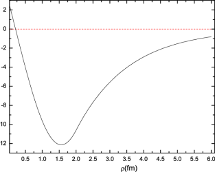
The functions $u_{1}(\rho)$ and $u_{2}(\rho)$ are shown in Fig.2 and Fig.3 respectively. From the figures, one can see that $u_{1}(\rho)$ is a sharply peaked curve with a maximum at $\rho=0$, and $u_{2}(\rho)$ has a node at $\rho\sim 0.3{\rm fm}$ and $|u_{2}(\rho)|$ has an absolute maximum at $\rho\sim 1.5{\rm fm}$. Both $u_{1}(\rho)$ and $u_{2}(\rho)$ satisfy the boundary condition given by Eq.(48).

Figure 2: The Wave Function $u_{1}(\rho)$.

Figure 3: The Wave Function $u_{2}(\rho)$.

In order to be sure of that the three-dimensional wave functions of our solutions can be normalized, we verify that

$$\int d^{3}{\bf x}|\psi_{i}({\bf x})|^{2} = \int d\Omega\int_{0}^{\infty}\rho^{2}d\rho{1\over\rho^{2}}|u_{i}(\rho)|^{2}=\int d\Omega\int_{0}^{\infty}d\rho|u_{i}(\rho)|^{2}$$

$$= 4\pi\left(\int_{0}^{a_{p\bar{p}}}d\rho|u_{i}(\rho)|^{2}+\int_{a_{p\bar{p}}}^{\infty}d\rho|u_{i}(\rho)|^{2}\right)$$

$$= 4\pi\left({\rm const.}+{\rm const.}\int_{a_{p\bar{p}}}^{\infty}d\rho e^{-2\sqrt{-m_{p}E_{i}}}\right)$$

$$= {\rm finite},$$

where $i=1,2$ and $u_{i}(\rho)$ have been given in eqs.(49), (50). Equation (A) is a check to the rationality of our solutions.

In the following, we discuss the the parameters in the model in order:

1. $a_{p\bar{p}}$ and $V_{p\overline{p}}$  : We take the width of the square well potential, denoted as $a_{p\bar{p}}$, as close to that of the deuteron, i.e., $a_{p\bar{p}}\sim a_{pn}\simeq 2.0~{}\mbox{fm}$. According to QCD inspired considerations Datta ; Maltman ; Rujula , the well potential between $q$ and $\bar{q}$ should be twice as attractive as the $q-q$-case, i.e., the depth of the $p\bar{p}$ square well potential is $V_{p\overline{p}}\simeq 2V_{pn}=73~{}\mbox{MeV}$.

2. $h$ and $\lambda$ : The quantitative results of the model somehow depend on the parameters of the potential, such as the barrier height $2m_{p}+h$ and width $\lambda$. For definiteness, we have taken them to be about $2m_{p}+m_{p}/4$ and $1/(2m_{p})$ in solving the Schr$\ddot{o}$dinger equation. Actually, this is reasonable because the dependence on height and width are weak in the practice calculation. The results with several different values for height and width are listed in Tables 1 and 2, where we see that the above values can give a reasonable binding energy $E_{2}$ and decay width $\Gamma_{X}$, in compatible with the BES measurement.

   
   

   barrier height $2m_{p}+h$	$2m_{p}+m_{p}/8$	$2m_{p}+m_{p}/6$	$2m_{p}+m_{p}/4$	$2m_{p}+m_{p}/2$	$2m_{p}+m_{p}$
   $E_{2}$	$-17.2~{}\mbox{MeV}$	$-17.2~{}\mbox{MeV}$	$-17.2~{}\mbox{MeV}$	$-17.3~{}\mbox{MeV}$	$-17.4~{}\mbox{MeV}$
   $\Gamma_{X}$	$17.7~{}\mbox{MeV}$	$16.8~{}\mbox{MeV}$	$15.5~{}\mbox{MeV}$	$12.7~{}\mbox{MeV}$	$9.7~{}\mbox{MeV}$

   TABLE 1: The binding energy $E_{2}$ and width $\Gamma$ obtained by solving the Skyrmion-type potential model with the potential barrier height $2m_{p}+h$ from $2m_{p}+m_{p}/8$ to $2m_{p}+m_{p}$.

   
   

   barrier width $\lambda$	$0.5/(2m_{p})$	$1/(2m_{p})$	$2/(2m_{p})$	$3/(2m_{p})$	$4/(2m_{p})$
   $E_{2}$	$-17.1~{}\mbox{MeV}$	$-17.2~{}\mbox{MeV}$	$-17.4~{}\mbox{MeV}$	$-17.4~{}\mbox{MeV}$	$-16.9~{}\mbox{MeV}$
   $\Gamma_{X}$	$19.3~{}\mbox{MeV}$	$15.5~{}\mbox{MeV}$	$9.9~{}\mbox{MeV}$	$6.4~{}\mbox{MeV}$	$4.2~{}\mbox{MeV}$

   TABLE 2: The binding energy $E_{2}$ and width $\Gamma$ obtained by solving the Skyrmion-type potential model with the potential barrier width $\lambda$ from $0.5/(2m_{p})$ to $4/(2m_{p})$ with $h=m_{p}/4$ fixed.

3. $c$ and $E_{1}$ : At $\rho\sim 0$, $V(\rho)\sim-c\;\delta(\rho)$ with a constant $c>0$, which is a free parameter in the model. $E_{1}$ is the eigenvalue of $u_{1}(\rho)$, which is roughly the energy level of the ${\rm Schr\ddot{o}dinger}$ equation with the one dimensional delta-function potential $V(\rho)\sim-c\;\delta(\rho)$. So, $E_{1}$ is $c$-dependent and, hence, once $E_{1}$ were fixed, the free parameter $c$ fixed. For definiteness, in this paper, we have taken

   $$E_{1}=-(2m_{p}-m_{\eta_{0}})\simeq-976~{}\mbox{MeV},$$ (61)

   and then the corresponding $c$ value is $c\simeq 2.161$ (see Eq.(58)).

References

- (1) J.Z.Bai et al.,Phys.Rev.Lett.91(2003)022001, hep-ex/0303006
- (2) K.Abe et al.,Phys.Rev.Lett.88, 181803(2002)
- (3) K.Abe et al.,Phys.Rev.Lett.89, 151802(2002)
- (4) E.Fermi and C.N.Yang,Phys.Rev.76, 1739(1949)
- (5) A.Datta and P.J. O’Donnell, Phys.Lett. B567, 273 (2003).
- (6) Mu-Lin Yan, Si Li, Bin Wu, Bo-Qiang Ma, hep-ph/0405087
- (7) Chong-Shou Gao and Shi-Lin Zhu, hep-ph/0308205.
- (8) J.L. Rosner, Phys. Rev. D68, 014004 (2003).
- (9) B.S.Zou and H.C.Chiang, Phys.Rev.D69(2004)034004; B.Kerbikov, A.Stavinsky and V.Fedotov , hep-ph/0402054.
- (10) R.D. Amado, F. Cannata, J-P. Dedonder, M.P. Locher, and B. Shao, Phys. Rev. Lett. 72, 970 (1994).
- (11) R.D. Amado, F.Cannata, J-P. Dedonder, M.P. Locher, and B. Shao, Phys.Rev.C50, 640-651, 1994, hep-ph/9403374
- (12) Yang Lu and R.D. Amado, Phys. Lett. B 357, 446 (1995); Phys. Rev. C 52, 2158 (1995).
- (13) J. Sedlk and V. , Sol. J. Part. Nucl. 19, 191 (1988).
- (14) C. Amsler and F. Myhrer, Annu. Rev. Nucl. Part. Sci. 41, 219 (1991).
- (15) H.M. Sommermann, R. Seki, S. Larson and S.E. Koonin, Phys. Rev. D45, 4303 (1992).
- (16) R.D. Amado, Nucl. Phys. B (proc. Suppl.) 56A 22-26 (1997); Nucl. Phys. A655, 236c-242c (1999).
- (17) R.D. Amado, F. Cannata, J.P. Dedonder, M.P. Locher, Yang Lu, Phys. Lett. B339, 201 (1994).
- (18) S.Ma, Rev. Mod. Phys. 25, 853 (1953); L. Hulthen and M. Sugawara, Handbuch der Physik 39, 1 (1959); L.I. Schiff, Quantum Mechanics, (McGraw-Hill Book Company, Inc., 1949).
- (19) T.H.R.Skyrme Proc.R.Soc.Lodon 262, 237(1961); Nucl.Phys, 31, 556(1962)
- (20) E.Witten, Nucl.Phys,B223,422(1983); B223,433(1983)
- (21) G.S.Adkins, C.R.Nappi, and E.Witten,Nucl.phys. B228, 552(1983)
- (22) K. Maltman and N. Isgur, Phys. Rev. D29,952(1984).
- (23) A. De Rujula, H. Georgi and S.L. Glashow, Phys. Rev. D12,147(1975).
- (24) Particle Data Group, Phys. Lett., B592, 1 (2004), (pp.519).
Appendix A
We solve the equation (3) with the toy model’s potential (1) (see Fig. 1) in the text. Namely, the potential ( note is at , is at , and ) is