Signature of the Minimal Supersymmetric Standard Model with Right-Handed Neutrinos in Long Baseline Experiments

Abstract

The effective interactions which violate a lepton flavor accompanied with neutrinos (nLFV) are considered. Such a new physics effect is expected to be measured in future neutrino oscillation experiments with long baseline. They are induced by radiative correction in the framework of the minimal supersymmetric standard model with right-handed neutrinos. We numerically evaluate the size of the couplings for nLFV interactions in this framework. The slepton mixing is not only the origin of the lepton flavor violation in the charged lepton sector (cLFV) but also that of the nLFV. We find that the nLFV couplings are strongly correlated with the corresponding cLFV process, and they are constrained at $\mathcal{O}(10^{-5})$ times smaller than the standard four-Fermi couplings.

I Introduction

Numerous observations on neutrinos from the sunsolar-r1 ; solar-r2 ; solar-r3 ; solar-r4 ; solar-sk ; solar-sno , the atmosphereatm1 ; atm2 ; atm3 , the reactorreactor , and the acceleratorK2K suggest that neutrinos are massive and hence there are mixings in the lepton sector. This fact means that the standard model (SM) has to be extended so that the neutrino masses and the lepton mixings are introduced into the model. Lots of models to explain those experimental results have been proposed. Among them, a model with the seesaw mechanismseesaw has a promising attribute, in which tiny neutrino masses are naturally induced. Neutrino experiments also have revealed that the mixings in the lepton sector are much larger than those in the quark sector. This fact may imply that the lepton flavor number is strongly violated in the physics beyond the SM. Therefore, we can expect that the nature might exhibit sizable lepton flavor violation (LFV) and hence we could observe the remains of physics at the high energy scale. In the minimal supersymmetric standard model with heavy right-handed neutrinos (MSSMRN), in which the seesaw mechanism is realized, the LFV with charged leptons (cLFV) is expected to become largeBM ; HMTYY ; MSSMRNcLFV . In this class of models, the renormalization effect due to the neutrino Yukawa couplings induces a significant size of off-diagonal elements of the slepton mass matrix, $(m^{2}_{\tilde{L}})_{\alpha}^{\ \beta}$ ($\alpha\neq\beta$, $\alpha,\beta=e,\mu,\tau$), which are the seeds of the cLFV. Here, the flavor indices $\alpha$ and $\beta$ should be understood to also indicate the mass eigenstates of the charged lepton fields. Concretely, the superpotential with the neutrino Yukawa couplings ${(f_{\nu})_{i}}^{\alpha}$ and the Majorana masses for the right-handed neutrinos $M^{ij}$ includes the following terms,

$$W\supset{(f_{\nu})_{i}}^{\alpha}\bar{N}^{i}H_{u}\epsilon L_{\alpha}+\frac{1}{2}M^{ij}N_{i}N_{j},$$ (1)

where $N_{i}$, $L_{\alpha}$, and $H_{u}$ denote the chiral supermultiplet for the right-handed neutrinos, that for the lepton doublets, and that for the up-type Higgs field, and $\epsilon$ is the anti-symmetric tensor for $SU(2)_{L}$ fundamental representation. The indices $i$ and $j$ are for the generation of right-handed neutrinos, which do not necessarily indicate the mass eigenstates. The renormalization group equation for the off-diagonal elements of the slepton mass matrix is given asBM ,

$$\mu\frac{{\rm d}(m^{2}_{\tilde{L}})_{\alpha}^{\ \beta}}{{\rm d}\mu}=\frac{1}{16\pi^{2}}\left[m^{2}_{\tilde{L}}f_{\nu}^{\dagger}f_{\nu}+f_{\nu}^{\dagger}f_{\nu}m^{2}_{\tilde{L}}+2(f_{\nu}^{\dagger}m^{2}_{\tilde{\nu}}f_{\nu}+\tilde{m}^{2}_{H_{u}}f_{\nu}^{\dagger}f_{\nu}+A_{\nu}^{\dagger}A_{\nu})\right]_{\alpha}^{\ \beta},\quad(\alpha\neq\beta),$$ (2)

where $m^{2}_{\tilde{\nu}}$ is the soft supersymmetry (SUSY) breaking mass matrix for the right-handed sneutrino, and $\tilde{m}^{2}_{H_{u}}$ is that for the up-type Higgs doublet. The matrix $A_{\nu}$ denotes the tri-linear scalar couplings corresponding to the first term in Eq. (1). Note that if the neutrino Yukawa couplings do not exist, then there is no LFV effect. We can approximately solve Eq. (2) as

$${(\Delta m^{2}_{\tilde{L}})}_{\alpha}^{\ \beta}\simeq-\frac{(6+2a_{0}^{2})m_{0}^{2}}{16\pi^{2}}(f_{\nu}^{\dagger}f_{\nu})_{\alpha}^{\ \beta}\ln\frac{M_{G}}{M_{R}},$$ (3)

with a cutoff scale $M_{G}$ and a typical mass scale for right-handed neutrinos $M_{R}$. Here, the universal soft SUSY breaking at $M_{G}$ is assumed, and $m_{0}$ is the parameter for sfermion masses and $a_{0}$ is that for scalar tri-linear couplings.

Figure 1: One of the diagrams which contribute to the cLFV process $l_{\beta}\rightarrow l_{\alpha}\gamma$. This effect is approximately understood by the insertion of the LFV mass term $(\Delta m^{2}_{\tilde{L}})_{\alpha}^{\ \beta}$ $(\alpha\neq\beta)$.

In terms of the mass insertion method, we can see that the off-diagonal elements of the slepton mass matrix are the origins of cLFV. This is diagrammatically shown in Fig. 1. From this diagram, it is obvious that the element $(\Delta m^{2}_{\tilde{L}})_{\alpha}^{\ \beta}$ is relevant to the process $l_{\beta}\rightarrow l_{\alpha}\gamma$. In this class of models, the off-diagonal elements can become large so that the typical values of predicted branching ratios are within a sensitivity reach of near future experimentsPSI ; MECO ; PRISM . Therefore, the search for the cLFV process is one of the promising ways to inspect the new physics effect beyond the SM.

In this article, however, we investigate an alternative approach to explore the LFV, the search for the processes of the LFV with neutrinos (nLFV) at a long baseline (LBL) neutrino oscillation experiment. In the forthcoming experiments, the oscillation parameters such as the mixing angles and the squared mass differences are expected to be determined with high precisionT2K ; nuFact ; combined . Therefore, the measurement of nLFV effects might be possible. The feasibility studies on the nLFV interaction search at future LBL experiments without assuming a specific model are made by Refs. Grossman ; GGGN ; NewPhysMatter ; HV ; HSV ; OSY ; OS ; Campanelli ; Tokushima ; Melbourne . The current experimental bounds on nLFV interactions are given in Ref. Davidson . The sensitivity for nLFV effects to solar neutrinosNSIinSolar , atmospheric neutrinosNSIinAtmos , the LSND resultsNSIinLSND and supernova neutrinosNSIinSN has also been considered. It is pointed out that the nLFV signal is enhanced by the interference effect between the amplitude including the nLFV interactions and that of the standard oscillation (SO).

We here investigate the nLFV interactions in the MSSMRN. The origins of nLFV processes are the same as those of cLFV processes, which are the off-diagonal elements of the slepton mass matrix. They can become significant in this framework. In addition, there is an enhancement mechanism due to the interference effect. It can be expected that the detectable magnitude of nLFV effects is induced. We make the numerical calculations of the size of the nLFV couplings and show the correlation between the nLFV and the cLFV.

In Sec. II, we recapitulate the model independent approach in the detection of nLFV effects at LBL neutrino oscillation experiments. We also show the way to parameterize the nLFV interactions. In Sec. III, we calculate these nLFV couplings in the MSSMRN and numerically evaluate the size of them under the universal soft SUSY breaking scenario, so-called the constrained MSSMRN. Here, we concentrate our attention on the nLFV interactions which are relevant in the oscillation channel $\nu_{\mu}\rightarrow\nu_{\tau}$. Finally, in Sec. IV we will give a summary. In Appendix A, we describe the model in order to make our notation clear, and in Appendix B we give formulae of the nLFV interactions.

II nLFV interaction in neutrino oscillation

In this section, we explain how to parameterize the new physics effect with the model independent wayOSY . First, we note that in neutrino oscillation experiments we do not observe neutrinos themselves but do their products, corresponding charged leptons. Propagating neutrinos appear only in intermediate states. Therefore, the existence of the nLFV interactions suggests that there are some amplitudes whose initial and final states are the same as those of the SO which means the neutrino oscillation with SM interactions.

To make the argument clear, we show an example. When we assume $\nu_{\mu}\rightarrow\nu_{\tau}$ oscillation measurement at a neutrino factory experiment, all we can know are the facts, the decay of muons at a muon storage ring and the appearance of tau leptons in a detector which is located at a length $L$ away from the source of the neutrino beam just after the time $L/c$, where $c$ is speed of light. We interpret these events as the evidence of the SO, $\nu_{\mu}\rightarrow\nu_{\tau}$. The amplitude for this process $A_{\rm SO}$ can be expressed by the product of the amplitudes for the sub-processes;

$$A_{\rm SO}(\mu^{-}+I\rightarrow\tau^{-}+F)=A_{s}(\mu^{-}\rightarrow\nu_{\mu}\bar{\nu}_{e}e^{-})A_{p}(\nu_{\mu}\xrightarrow[]{\text{osc.}}\nu_{\tau})A_{d}(\nu_{\tau}d\rightarrow\tau^{-}u),$$ (4)

where $I$ ($F$) denotes all the other particles than a muon (tau lepton) in the initial (final) state, which can be measured in principle. In this example, $I$ is $d$ (a down-type quark) in $A_{d}$, and $F$ means $\bar{\nu}_{e}$ and $e^{-}$ in $A_{s}$ and $u$ (a up-type quark) in $A_{d}$. The subscripts, $s,p$, and $d$, indicate “at the source of the neutrino beam”, “at the propagation process”, and “at the detection process”, respectively. Suppose that there is an effective four-Fermi nLFV interaction,

$$\mathcal{L}_{\text{eff}}=\lambda(\bar{e}\gamma^{\rho}{\rm P}_{L}\mu)(\bar{\nu}_{\tau}\gamma_{\rho}{\rm P}_{L}\nu_{e})+\ \hbox{\rm h.c.},$$ (5)

we have the same signal through the other process than Eq. (4);

$$A_{\rm nLFV}(\mu^{-}+I\rightarrow\tau^{-}+F)=A_{s}(\mu^{-}\rightarrow\nu_{\tau}\bar{\nu}_{e}e^{-})A_{p}(\nu_{\tau}\xrightarrow[]{\text{no osc.}}\nu_{\tau})A_{d}(\nu_{\tau}d\rightarrow\tau^{-}u).$$ (6)

The external particles in Eq. (6) are completely the same as those in Eq. (4). Therefore, we can not distinguish the contributions from these two amplitudes. In quantum mechanics, we first sum up these amplitudes and next square the summation in order to obtain the transition rate. Therefore, an interference term arises between these two amplitudes for this process:

$$P({\mu^{-}+I\rightarrow\tau^{-}+F})=|A_{\rm SO}|^{2}+2{\rm Re}[A_{\rm SO}^{*}A_{\rm nLFV}]+|A_{\rm nLFV}|^{2}.$$ (7)

The term of the SO, the first term of the right-hand side, gives the leading contribution, and it is described by using the muon decay width $\Gamma$ $(=|A_{s}(\mu^{-}\rightarrow\nu_{\mu}\bar{\nu}_{e}e^{-})|^{2})$ and the cross-section for the charged current interaction $\sigma$ $(=|A_{d}(\nu_{\tau}d\rightarrow\tau^{-}u)|^{2})$ as

$$\left|A_{\rm SO}\right|^{2}=\Gamma\times P_{\nu_{\mu}\rightarrow\nu_{\tau}}\times\sigma,$$ (8)

where $P_{\nu_{\mu}\rightarrow\nu_{\tau}}$ is the oscillation probability for $\nu_{\mu}\rightarrow\nu_{\tau}$ in the SO, which is defined as $|A_{p}(\nu_{\mu}\xrightarrow[]{\text{osc.}}\nu_{\tau})|^{2}$. The second term which represents the interference between the amplitude of the SO Eq. (4) and that including the nLFV interaction Eq. (6):

$$2\text{Re}[A_{\rm SO}^{*}A_{\text{nLFV}}]=\Gamma\times 2\text{Re}\left[\frac{\lambda}{2\sqrt{2}G_{F}}A_{p}^{*}(\nu_{\mu}\xrightarrow[]{\text{osc.}}\nu_{\tau})A_{p}(\nu_{\tau}\xrightarrow[]{\text{no osc.}}\nu_{\tau})\right]\times\sigma,$$ (9)

where $G_{F}$ is the Fermi constant. Note that the nLFV effect contributes to the oscillation probability not quadratically but linearly. Thus the effect can be enhanced and hence even if the nLFV coupling is small, it can contribute the oscillation probability significantlyHSV ; OSY ; OS .

We now turn to the parametrization of effective couplings for nLFV interactions. As we have already shown, the amplitude for the neutrino oscillation process can be divided into three pieces, $A_{s}$, $A_{p}$, and $A_{d}$. First, we consider the decay process of parent particles, $A_{s}$. Since all final states must be the same, nLFV interactions with $(V-A)(V-A)$ type are important for the neutrino factory experimentOSY . We can introduce the interference effect by treating the initial state of a propagating neutrino as the superposition of all flavor eigenstates. For the case of Eq. (5), we can take the initial neutrino state $|\nu\rangle$ as

$$|{\nu}\rangle=|{\nu}_{\mu}\rangle+\epsilon^{s}_{\mu\tau}|{\nu}_{\tau}\rangle.$$ (10)

where $\epsilon^{s}_{\mu\tau}=\lambda/(2\sqrt{2}G_{F})$. It can be generalized to the case of an initial neutrino with any flavor by using the source state notation which is introduced in Ref. Grossman as

$$|\nu^{s}_{\beta}\rangle={(U^{s})_{\beta}}^{\alpha}|\nu_{\alpha}\rangle,\qquad U^{s}\equiv\left(\begin{array}[]{ccc}1&\epsilon^{s}_{e\mu}&\epsilon^{s}_{e\tau}\\ \epsilon^{s}_{\mu e}&1&\epsilon^{s}_{\mu\tau}\\ \epsilon^{s}_{\tau e}&\epsilon^{s}_{\tau\mu}&1\end{array}\right).$$ (14)

We can include the total nLFV effect into the oscillation probability as

$$P_{\nu^{s}_{\alpha}\rightarrow\nu_{\beta}} =\left|\langle\nu^{\beta}|{\left({\rm e}^{-{\rm i}H_{\rm SO}L}\right)_{\beta}}^{\alpha}{\left(U^{s}\right)_{\alpha}}^{\gamma}|\nu_{\gamma}\rangle\right|^{2},$$ (15)

with the propagation Hamiltonian for the SO $H_{\rm SO}$;

$${(H_{\rm SO})_{\beta}}^{\alpha}=\frac{1}{2E_{\nu}}\left\{{\left(U_{\rm MNS}\right)_{\beta}}^{i}\left(\begin{array}[]{ccc}0&&\\ &\Delta m_{21}^{2}&\\ &&\Delta m_{31}^{2}\end{array}\right){\left(U_{\rm MNS}^{\dagger}\right)_{i}}^{\alpha}+{\left(\begin{array}[]{ccc}\bar{a}&&\\ &0&\\ &&0\end{array}\right)_{\beta}}^{\alpha}\right\},$$ (22)

where $E_{\nu}$ is the neutrino energy, $\bar{a}$ is the usual matter effect which is given as $2\sqrt{2}G_{F}n_{e}E_{\nu}$ by using the electron number density $n_{e}$, $U_{\rm MNS}$ is the mixing matrix for the lepton sector, and $\Delta m^{2}_{21}$ ($\Delta m^{2}_{31}$) is the mass squared difference for the solar (atmospheric) neutrino oscillation.

Next, we consider the propagation process, $A_{p}$. The nLFV interactions modify the Hamiltonian for neutrino propagation asNewPhysMatter ,

$${(H_{\rm nLFV})_{\beta}}^{\alpha}={(H_{\rm SO})_{\beta}}^{\alpha}+\frac{1}{2E_{\nu}}{\begin{pmatrix}a_{ee}&a_{e\mu}&a_{e\tau}\\ a_{e\mu}^{*}&a_{\mu\mu}&a_{\mu\tau}\\ a_{e\tau}^{*}&a_{\mu\tau}^{*}&a_{\tau\tau}\end{pmatrix}_{\beta}}^{\alpha},$$ (23)

where $a_{\alpha\beta}$ is the extra matter effect due to nLFV interactions, which is defined as $a_{\alpha\beta}=\sum_{p=e,d,u}2\sqrt{2}\epsilon^{m,p}_{\alpha\beta}G_{F}n_{p}E_{\nu},$ where $n_{p}$ is the number density for the particle $p$. Assuming the matter which consists of the same number of electron, neutron and proton, we can reduce it to

$$a_{\alpha\beta}=2\sqrt{2}\epsilon^{m}_{\alpha\beta}G_{F}n_{e}E_{\nu},$$ (24)

with

$$\epsilon^{m}_{\alpha\beta}\equiv\epsilon^{m,e}_{\alpha\beta}+3\epsilon^{m,d}_{\alpha\beta}+3\epsilon^{m,u}_{\alpha\beta}.$$ (25)

Note that to consider the magnitude of the matter effect, the type of the interaction is irrelevant since matter particles are at rest and hence the dependence on their chirality is averaged outBGE .

Then, we make a comment on nLFV interactions which affect a detection process, $A_{d}$. We can adopt a quite similar treatment to that at the source of the neutrino beam. In this article, we consider the case in which the nLFV interactions do not depend on the flavor of target-quark, which is almost the case for the so-called constrained MSSMRN. Therefore, we have the neutrino state for the detection process in the following form,

$$|\nu^{d}_{\beta}\rangle={(U^{d})_{\beta}}^{\alpha}|\nu_{\alpha}\rangle,\qquad U^{d}\equiv\left(\begin{array}[]{ccc}1&\epsilon^{d}_{e\mu}&\epsilon^{d}_{e\tau}\\ \epsilon^{d}_{\mu e}&1&\epsilon^{d}_{\mu\tau}\\ \epsilon^{d}_{\tau e}&\epsilon^{d}_{\tau\mu}&1\end{array}\right).$$ (29)

Finally, the transition probability including the whole nLFV effects is given as

$$P(\mu^{-}+I\rightarrow\tau^{-}+F)\simeq\Gamma\times P_{\nu^{s}_{\alpha}\rightarrow\nu_{\beta}^{d}}\times\sigma,$$ (30)

where

$$P_{\nu^{s}_{\alpha}\rightarrow\nu_{\beta}^{d}} =\left|\langle\nu^{\delta}|{(U^{d\dagger})_{\delta}}^{\beta}{({\rm e}^{-{\rm i}H_{\text{nLFV}}L})_{\beta}}^{\alpha}{(U^{s})_{\alpha}}^{\gamma}|\nu_{\gamma}\rangle\right|^{2}.$$ (31)

III nLFV interactions in the MSSMRN

In this section, we evaluate the effective couplings for nLFV interactions in the MSSMRN. The nLFV interactions are induced by the off-diagonal elements of the slepton mass matrix, which are similar to the cLFV interactions. We can naively estimate the size of the nLFV parameter $\epsilon^{s}_{\alpha\beta}$ from the diagram which is shown in Fig. 2 asosNufact04

$$\epsilon^{s}_{\alpha\beta}\left(\sim\epsilon^{s}_{\beta\alpha}\right)\sim\frac{g^{2}_{2}}{16\pi^{2}}\frac{{(\Delta m^{2}_{\tilde{L}})_{\beta}}^{\alpha}}{m_{\rm S}^{2}}\sim m_{\rm S}^{2}\times\sqrt{\text{Br}(l_{\beta}\rightarrow l_{\alpha}\gamma)}.$$ (32)

Here $g_{2}$ is the gauge coupling for $SU(2)_{L}$ and $m_{\rm S}$ is the typical SUSY breaking scale.

Figure 2: One of the diagrams which contribute to $\epsilon^{s}_{\beta\alpha}$.

This relation means that there is a correlation between two processes, $\l^{-}_{\beta}\rightarrow\nu_{\alpha}\bar{\nu}_{e}e^{-}$ and $l_{\beta}\rightarrow l_{\alpha}\gamma$. We here concentrate our attention on the nLFV associated with the tau lepton because that in $\mu$-$e$ sector is strongly constrained by corresponding cLFV processes. The current experimental bound on the branching ratio of $\tau\rightarrow\mu\gamma$ is $3.1\times 10^{-7}$ at 90% confidence levelBelle-tmg , and then this experimental bound constrains the nLFV coupling parameter $\epsilon^{s}_{\mu\tau}$. According to this naive estimation, the value of $\epsilon^{s}_{\mu\tau}$ may become as large as $\mathcal{O}(10^{-4})$. Such size of nLFV interactions would be detected at a future LBL experiment such as the neutrino factoryOSY .

III.1 Analytic Calculation of $\epsilon^{s,m,d}_{\alpha\beta}$

In this subsection, we explain the calculation to obtain $\epsilon^{s,m,d}_{\alpha\beta}$ in detail and compare them with that of cLFV processes. The thorough results are given in Appendix B.

For example, the effective Lagrangian relevant with the nLFV interactions which give potentially significant contribution to the oscillation $\nu_{\mu}\rightarrow\nu_{\tau}$ in a neutrino factory is given asOSY

$$\mathcal{L}^{\text{nLFV}}_{\text{eff}}= 2\sqrt{2}G_{F}\epsilon^{s}_{\mu\tau}\left(\bar{\nu}_{\tau}\gamma^{\rho}{\rm P}_{L}\nu_{e}\right)\left(\bar{e}\gamma_{\rho}{\rm P}_{L}\mu\right)$$

$$+2\sqrt{2}G_{F}\sum_{p=e,d,u}\epsilon^{m,p}_{\mu\tau}\left(\bar{\nu}_{\tau}\gamma^{\rho}{\rm P}_{L}\nu_{\mu}\right)\left(\bar{p}\gamma_{\rho}p\right)$$ (33)

$$+2\sqrt{2}G_{F}\epsilon^{d}_{\mu\tau}\left(\bar{\tau}\gamma^{\rho}{\rm P}_{L}\nu_{\mu}\right)\left(\bar{u}\gamma_{\rho}{\rm P}_{L}d\right).$$

These effective couplings arise from penguin-type diagrams and from box-type diagrams as shown in Appendix B. The calculation of box diagrams is straightforward. It is almost the same as that of cLFV processes, e.g., $\mu$-$e$ conversionHMTYY except for the fact that only the $(V-A)(V-A)$ type interactions are taken into account in the calculation of $\epsilon^{s}_{\alpha\beta}$ and $\epsilon^{d}_{\alpha\beta}$. However, it is necessary to make an attentive calculation for penguin-type diagrams. In general, while the neutral and electromagnetic currents corresponding to Fig. 1 take the following form,

$$\bar{f}^{\alpha}(p-q)\left[{\rm i}\left\{\mathfrak{A}(q^{2})+\mathfrak{B}(q^{2})\gamma_{5}\right\}q_{\nu}\sigma^{\mu\nu}+\left\{\mathfrak{C}(q^{2})+\mathfrak{D}(q^{2})\gamma_{5}\right\}\gamma^{\mu}+\left\{\mathfrak{E}(q^{2})+\mathfrak{F}(q^{2})\gamma_{5}\right\}q^{\mu}\right]f_{\beta}(p)$$

$$+{\rm h.c.},$$ (34)

the charged current corresponding to Fig. 2 is decomposed to

$$\bar{\nu}^{\alpha}(p-q){\rm P}_{R}\left\{{\rm i}\mathfrak{A}^{\prime}(q^{2})q_{\nu}\sigma^{\mu\nu}+\mathfrak{C}^{\prime}(q^{2})\gamma^{\mu}+\mathfrak{E}^{\prime}(q^{2})q^{\mu}\right\}l_{\beta}(p)+{\rm h.c.}.$$ (35)

Here, $f$ denotes the charged lepton field $l$ or the neutrino field $\nu$, $p$ is the momentum for the incoming particle, and $q$ is that for the gauge boson. All the coefficients, $\mathfrak{A}$ ($\mathfrak{A}^{\prime}$), $\mathfrak{B}$, $\mathfrak{C}$ ($\mathfrak{C}^{\prime}$), $\mathfrak{D}$, $\mathfrak{E}$ ($\mathfrak{E}^{\prime}$), and $\mathfrak{F}$, are the functions of $q^{2}$. In the limit $q^{2}\rightarrow 0$, $\mathfrak{C}$ and $\mathfrak{D}$ for the electromagnetic current must vanish due to the gauge symmetry $U(1)_{\rm em}$. On the other hand, those for the neutral and the charged current do not vanish because the corresponding gauge symmetry $SU(2)_{L}$ is broken. In other words, the Lorentz structure of the nLFV interaction which is shown in Fig. 2 is different from that of the cLFV process $l_{\beta}\rightarrow l_{\alpha}\gamma$ with a real photon emission. The former one is dominated by the vector exchange interaction ($\mathfrak{C}^{\prime}(0)$), while the latter is done by a di-pole type interaction ($\mathfrak{A}(0)+\mathfrak{B}(0)\gamma_{5}$). Therefore, they are definitely correlated each other but are not the same functions.

Figure 3: One example of the diagrams in which we have to take into account the off-shellness for the neutrino propagation. In the neutrino propagator which is pointed out by the oval, we must treat the neutrino as if it were a massless particle.

In the calculation of nLFV diagrams, we have to pay attention to the following two facts: (i) we regard neutrinos as highly off-shell particle, and (ii) we must avoid counting one contribution twice. First, we explain the reason why neutrinos behave as highly off-shell particles, and hence it is necessary to treat that neutrinos are massless in diagrams for effective nLFV interactions. In Fig. 3, from the viewpoint of the uncertainty principle, the condition for neutrino oscillation to occur is described asFY

$$\delta(p-q)\sim\frac{1}{\delta x} \gg \frac{1}{L}\sim\frac{\Delta m^{2}}{p-q},$$ (36)

where $\delta x$ is the uncertainty of the position and the time in which neutrinos are produced, $\delta(p-q)$ is the uncertainty of the energy-momentum of the outgoing neutrino, and $\Delta m^{2}$ is the neutrino mass squared difference corresponding to the LBL oscillation experiment. The inequality results from the fact that the neutrino production position must be determined much more accurately than the baseline length $L$. The fact that the neutrino oscillation phenomena are observed in the LBL experiment requires that the equality at the most right-hand side should be satisfied. Thus, the uncertainty of the squared momentum must conform to the following relation

$$\delta\{(p-q)^{2}\} \gg \Delta m^{2}\qquad\text{then}\qquad\langle(p-q)^{2}\rangle\gg m^{2}_{\nu},$$ (37)

where $\langle(p-q)^{2}\rangle$ denotes the average of $(p-q)^{2}$. This inequation shows that the average of the neutrino momentum is much larger than its mass, and it follows from this that neutrinos are generally highly off-shell fields in oscillation experiments. This also means that all the diagrams for the nLFV interactions include the off-shell neutrino as external lines. In the exact meaning of the field theory, we do not have the method to calculate diagrams with off-shell external legs. However, we can evaluate such diagrams by treating as if the neutrinos were massless. For the practical purpose, we make the following replacement which we refer as the off-shell prescription in calculations of the type of diagram shown in Fig. 3;

$$\frac{(p-q)^{2}}{(p-q)^{2}-m_{\nu_{\beta}}^{2}}\Longrightarrow\begin{cases}1,&\hbox{(off-shell prescription)},\\ \frac{m_{\nu_{\alpha}}^{2}}{m_{\nu_{\alpha}}^{2}-m_{\nu_{\beta}}^{2}},&\hbox{(for usual on-shell particle case)}.\end{cases}$$ (38)

Next, we turn to the problem of the double counting and show the way to solve it. First, we note that we must calculate the process $\mu^{-}+I\rightarrow\tau^{-}+F$ with the method of the field theory, so that we must not calculate the nLFV effect for each stage because we cannot observe the each stage separately.

Figure 4: Schematic explanation for the double counting problem. If we count the diagram-(a) into $\epsilon^{s}_{\mu\tau}$ and we also do the diagram-(b) into $\epsilon^{m}_{\mu\tau}$, then we count the diagram-(c) twice.

If we calculate the diagrams shown in Figs. 4-(a) for $\epsilon^{s}_{\mu\tau}$ and 4-(b) for $\epsilon^{m}_{\mu\tau}$, then it means that we count twice the diagram of Fig. 4-(c) into the calculation of the process $\mu^{-}+I\rightarrow\tau^{-}+F$. In order to avoid doubly counting, we have to get rid of one of them. For example, we should not include the contribution of the diagram of Fig. 4-(b) in $\epsilon^{m}_{\mu\tau}$. A similar situation occurs among $\epsilon^{d}_{\mu\tau}$ and $\epsilon^{m}_{\mu\tau}$. The penguin contribution to $\epsilon^{d}_{\mu\tau}$ is essentially given by the complex conjugate of that to the corresponding $\epsilon^{s}_{\tau\mu}$. However, we must eliminate the contribution from diagrams similar to Fig. 4-(a) from $\epsilon^{d}_{\mu\tau}$.

Finally, we should notice another thing that is important for the double counting problem; Which stage (source or matter) does the contribution of Fig. 4-(c) belong to? For example, instead of removing the contribution of Fig. 4-(b) in $\epsilon^{m}_{\mu\tau}$, we can eliminate the contribution of Fig. 4-(a) in $\epsilon^{s}_{\mu\tau}$. For this ambiguity, we adopt the way to divide the diagram into each stage so that epsilon parameters in each stage will disappear in the limit where $m_{\rm S}\rightarrow\infty$ after using the off-shell prescription. The $SU(2)_{L}$ symmetry is recovered and then $\epsilon^{s,m,d}_{\mu\tau}$ should disappear in the large SUSY scale limit. This is shown analytically. Note that each diagram gives rather large contribution and stays almost constant in the large SUSY scale limit. The cancellation among the diagrams is highly nontrivial. Therefore, by checking the cancellation among the diagrams, we can be confident about the legitimacy of our treatment for the internal neutrino lines.

III.2 Numerical Study

A numerical study to evaluate the epsilon parameters is necessary in order to make it clear whether our naive estimation Eq. (32) is correct. We here assume the universal soft SUSY breaking at $M_{G}$ and adopt the scenario of the radiative electroweak symmetry breakingIKKT . The detail of calculations is shown in Appendices. We scan the values for the soft SUSY breaking parameters $m_{0}$ and $M_{1/2}$ at the range of 100 - 1,000 GeV, and also scan the elements of the neutrino Yukawa matrix. We here take the normal hierarchy for the neutrino mass matrix. The scatter plots for size of $\epsilon^{s}_{\mu\tau}$, $\epsilon^{m}_{\mu\tau}$ and $\epsilon^{d}_{\mu\tau}$ are presented in Fig. 5.

Figure 5: Scatter plots for size of nLFV parameters $\epsilon^{s}_{\mu\tau}$, $\epsilon^{m}_{\mu\tau}$ and $\epsilon^{d}_{\mu\tau}$. Dots are for $\tan\beta=10$ and triangles are for $\tan\beta=3$. We here fix the soft SUSY breaking parameters as $a_{0}=0$ and $\mu>0$.

All of them take similar behavior. As expected from Eq. (32), the nLFV parameters correlate with the branching ratio of the process $\tau\rightarrow\mu\gamma$. However, the size of the parameters is much smaller than that of the naive estimation. This fact can be understood by the cancellation among the diagrams which contribute to the nLFV interaction. In the $SU(2)_{L}$ symmetric limit, the diagrams for the penguin contribution to the nLFV interaction must cancel each other out because of the gauge symmetry. Since the diagrams for nLFV interactions are induced at the $m_{\rm S}$ scale, in the limit where $m_{\rm S}\gg m_{Z}$, the $SU(2)_{L}$ symmetry is assumed to be recovered. Even in the case where $m_{\rm S}\sim\mathcal{O}(100)$ GeV, the cancellation is rather significant. Thus, our naive estimation must be modified so that the additional suppression factor $m_{Z}/m_{\rm S}$ is introduced. It may be worth pointing out that the epsilon parameters do not strongly depend on the value of $\tan\beta$ unlike the branching ratio of the cLFV process. This fact arises from the difference in the structure of the chirality in each process. The process $\tau\rightarrow\mu\gamma$ is dominated by the diagrams including the left-right mixing of the slepton which is proportional to $\tan\beta$. The nLFV processes do not pick up such the left-right mixing term because a chirality flip is not necessary. Therefore, nLFV search may be advantageous in the case where $\tan\beta$ is relatively small. We also note that it is obvious from Eq. (3) that both nLFV and cLFV are enhanced when $a_{0}$ takes a large value.

IV Summary

We summarize our study and give some discussions. It is known that magnitude of nLFV couplings can become large enough to be detected at future LBL experiments within model-independent approach. We here considered the nLFV interactions in the MSSMRN under the universal soft SUSY breaking scenario which is one of the most promising candidates for the physics beyond the SM.

We find that in this scenario the nLFV couplings cannot be significant, and hence it is quite difficult to observe these effects at future oscillation experiments. The reason why they are strongly suppressed is that the $SU(2)_{L}$ gauge symmetry is approximately maintained. All the particles and the interactions which can generate nLFV interactions respect the $SU(2)_{L}$ symmetry in the limit $m_{S}\rightarrow\infty$. Although each diagram to contribute to nLFV interactions can become large, a brilliant cancellation among those diagrams occurs. Therefore, the penguin contributions are strongly suppressed.

We adopt the approximation for the calculation of penguin diagrams which is explained in Sec. III.1. In order to confirm the validity of this approximation, we need to make the calculation for the process shown in Fig. 4-(c) by using the method of the field theory. However, the calculation which we adopt here must be reliable in the sense of the field theory because the consistencies, i.e., the recovery of $SU(2)_{L}$ gauge symmetry, are obviously maintained in our calculation.

Finally, we mention our future work. Since the decay process of a muon differs from that of a pion, we might expect that sizable new physics effect exists only in the decay of pion. Thus, it is necessary to investigate nLFV effects in the MSSMRN at superbeam experiments individually. Furthermore, because within the model independent approach, epsilon parameters can be still significant and there are lots of the other models than the constrained MSSMRN which can explain the neutrino masses and the lepton mixings, we need to examine such possibilities.

Acknowledgments
J. S. thanks J. W. F. Valle for useful discussion. The work of T. O. is supported in part by Japan Society for Promotion of Science No. 3693. J. S. was supported by the Grant-in-Aid for Scientific Research on Priority Area No.16038202 and 14740168.

Appendix A Model

We basically follow the notation which is adopted in Ref. HMTYY . However, we pay attention to the fact that the mixing matrices to diagonalize the mass matrices for sferimons, chargino and neutralino are complex matrices, in general.

The mass matrices for charged slepton, down-type squark and up-type squark are

$$-\mathcal{L}_{\tilde{f}}= \begin{pmatrix}\tilde{f}_{L}^{*}&\tilde{f}_{R}^{*}\end{pmatrix}^{\alpha}{\left(M_{\tilde{f}}^{2}\right)_{\alpha}}^{\beta}\begin{pmatrix}\tilde{f}_{L}\\ \tilde{f}_{R}\end{pmatrix}_{\beta}=\begin{pmatrix}\tilde{f}_{L}^{*}&\tilde{f}_{R}^{*}\end{pmatrix}\begin{pmatrix}M_{\tilde{f}_{LL}}^{2}&(M_{\tilde{f}_{LR}}^{2})^{\dagger}\\ M_{\tilde{f}_{LR}}^{2}&M_{\tilde{f}_{RR}}^{2}\end{pmatrix}\begin{pmatrix}\tilde{f}_{L}\\ \tilde{f}_{R}\end{pmatrix},$$ (39)

where

$$M_{\tilde{f}_{LL}}^{2} =\begin{cases}m_{\tilde{f}_{L}}^{2}+\left(f_{f}^{\dagger}f_{f}\right)\frac{v^{2}}{\sqrt{2}}\sin^{2}\beta+m_{Z}^{2}\cos 2\beta\left\{\left(\frac{1}{2}\right)-Q^{f}_{\rm em}\sin^{2}\theta_{W}\right\},\qquad\text{($f=u$)},\\ m_{\tilde{f}_{L}}^{2}+\left(f_{f}^{\dagger}f_{f}\right)\frac{v^{2}}{\sqrt{2}}\cos^{2}\beta+m_{Z}^{2}\cos 2\beta\left\{\left(-\frac{1}{2}\right)-Q^{f}_{\rm em}\sin^{2}\theta_{W}\right\},\quad\text{($f=l,d$)},\end{cases}$$ (40)

$$M_{\tilde{f}_{RR}}^{2} =\begin{cases}m_{\tilde{f}_{R}}^{2}+\left(f_{f}f_{f}^{\dagger}\right)\frac{v^{2}}{\sqrt{2}}\sin^{2}\beta-m_{Z}^{2}\cos 2\beta\left\{-Q^{f}_{\rm em}\sin^{2}\theta_{W}\right\},\qquad\text{($f=u$)},\\ m_{\tilde{f}_{R}}^{2}+\left(f_{f}f_{f}^{\dagger}\right)\frac{v^{2}}{\sqrt{2}}\cos^{2}\beta-m_{Z}^{2}\cos 2\beta\left\{-Q^{f}_{\rm em}\sin^{2}\theta_{W}\right\},\qquad\text{($f=l,d$)},\end{cases}$$ (41)

$$M_{\tilde{f}_{LR}} =\begin{cases}-A_{f}\frac{v}{\sqrt{2}}\sin\beta-\mu f_{f}\frac{v}{\sqrt{2}}\sin\beta\cot\beta,\qquad\text{($f=u$)},\\ A_{f}\frac{v}{\sqrt{2}}\cos\beta-\mu f_{f}\frac{v}{\sqrt{2}}\cos\beta\tan\beta,\qquad\text{($f=l,d$)}.\end{cases}$$ (42)

Here, the indices $\alpha$ and $\beta$ are for interaction eigenstates for thier superpartner fermion fields. We take the basis where the mass matrix for the charged lepton field is diagonal, so that the index for chraged lepton indicates its interaction eigenstate and its mass eigenstate, simultaneously. The unitary matrix $U_{\tilde{f}}$ is defined as

$${(U_{\tilde{f}})_{X}}^{\alpha}{(M_{\tilde{f}}^{2})_{\alpha}}^{\beta}{(U_{\tilde{f}}^{\dagger})_{\beta}}^{Y}=\text{diag}(m_{\tilde{f}_{X}}^{2}){\delta_{X}}^{Y}.$$ (43)

The relations between the mass eigenstates and the interaction eigenstates are

$$\tilde{f}_{X}={(U_{\tilde{f}})_{X}}^{\alpha}\tilde{f}_{L\alpha}+{(U_{\tilde{f}})_{X}}^{\alpha+3}\tilde{f}_{R\alpha},$$ (44)

$$\tilde{f}_{L\alpha}={(U_{\tilde{f}}^{\dagger})_{\alpha}}^{X}\tilde{f}_{X},\qquad\tilde{f}_{R\alpha}={(U_{\tilde{f}}^{\dagger})_{\alpha+3}}^{X}\tilde{f}_{X}.$$ (45)

The sneutrino mass term is also given as

$$-\mathcal{L}_{\tilde{\nu}}=\tilde{\nu}^{*\alpha}{(M_{\tilde{\nu}}^{2})_{\alpha}}^{\beta}\tilde{\nu}_{\beta},$$ (46)

where

$$(M_{\tilde{\nu}}^{2})=m_{\tilde{L}}^{2}+m_{\nu}^{\dagger}m_{\nu}+m_{Z}^{2}\cos 2\beta\left(\frac{1}{2}\right),$$ (47)

where $m_{\nu}$ is the neutrino mass matrix which is induced by the seesaw mechanism;

$$m_{\nu}=f_{\nu}^{\sf T}M^{-1}f_{\nu}\frac{v^{2}}{2}\sin\beta.$$ (48)

The unitary matrix $U_{\tilde{\nu}}$ is defined as

$${(U_{\tilde{\nu}})_{X}}^{\alpha}{(M_{\tilde{\nu}}^{2})_{\alpha}}^{\beta}{(U_{\tilde{\nu}}^{\dagger})_{\beta}}^{Y}=\text{diag}(m_{\tilde{\nu}_{X}}^{2}){\delta_{X}}^{Y}.$$ (49)

The relations between the mass eigenstates and the interaction eigenstates are

$$\tilde{\nu}_{X}={(U_{\tilde{\nu}})_{X}}^{\alpha}\tilde{\nu}_{L\alpha},\qquad\tilde{\nu}_{L\alpha}={(U_{\tilde{\nu}}^{\dagger})_{\alpha}}^{X}\tilde{\nu}_{X}.$$ (50)

The chargino mass term in the 2-spinor representation is

$$-\mathcal{L}_{\tilde{\chi}^{-}}=\begin{pmatrix}\tilde{w}^{+}&\tilde{h}_{u}^{+}\end{pmatrix}^{i}{\left(M_{C}\right)_{i}}^{j}\begin{pmatrix}\tilde{w}^{-}\\ \tilde{h}_{d}^{-}\end{pmatrix}_{j}=\begin{pmatrix}\tilde{w}^{+}&\tilde{h}_{u}^{+}\end{pmatrix}\begin{pmatrix}M_{2}&\sqrt{2}m_{W}\cos\beta\\ \sqrt{2}m_{W}\sin\beta&\mu\end{pmatrix}\begin{pmatrix}\tilde{w}^{-}\\ \tilde{h}_{d}^{-}\end{pmatrix}.$$ (51)

The diagonalization is done by unitary matrices $U_{R}$ and $U_{L}$ as

$${(U_{R})_{A}}^{i}{(M_{C})_{i}}^{j}{(U_{L}^{\dagger})_{j}}^{B}=\text{diag}(M_{\tilde{\chi}^{-}_{A}}){\delta_{A}}^{B},$$ (52)

The relations between the interaction eigenstates and the mass eigenstates are

$$(\tilde{x}^{-}_{A})_{a}={(U_{L})_{A}}^{i}\begin{pmatrix}(\tilde{w}^{-})_{a}\\ (\tilde{h}_{d}^{-})_{a}\end{pmatrix}_{i},\qquad(\tilde{x}^{+A})_{a}={(U_{R}^{*})^{A}}_{i}\begin{pmatrix}(\tilde{w}^{+})_{a}\\ (\tilde{h}_{u}^{+})_{a}\end{pmatrix}^{i},$$ (53)

where $a$ ($\dot{a}$) denotes index for the Lorentz spinor for ${\bf 2}$ ($\bf{\bar{2}}$) under $SL(2,C)$. We here adopt the same rule as that in Ref. HaberKane . The 4-spinors for mass eigenstates are constructed as

$$\tilde{\chi}^{-}_{A}=\begin{pmatrix}(\tilde{x}^{-}_{A})_{a}\\ (\overline{\tilde{x}^{+}}_{A})^{\dot{a}}\end{pmatrix},\qquad\tilde{\chi}^{+A}=\begin{pmatrix}(\tilde{x}^{+A})_{a}\\ (\overline{\tilde{x}^{-}}^{A})^{\dot{a}}\end{pmatrix},$$ (54)

and then those for interaction eigenstates are

$$\tilde{W}^{-} =\begin{pmatrix}(\tilde{w}^{-})_{a}\\ (\overline{\tilde{w}^{+}})^{\dot{a}}\end{pmatrix}=\begin{pmatrix}{(U_{L}^{\dagger})_{1}}^{A}(\tilde{x}^{-}_{A})_{a}\\ {(U_{R}^{\dagger})_{1}}^{A}(\overline{\tilde{x}^{+}}_{A})^{\dot{a}}\end{pmatrix},\qquad\tilde{W}^{+}=\begin{pmatrix}(\tilde{w}^{+})_{a}\\ (\overline{\tilde{w}^{-}})^{\dot{a}}\end{pmatrix}=\begin{pmatrix}{(U_{R}^{\sf T})^{1}}_{A}(\tilde{x}^{+A})_{a}\\ {(U_{L}^{\sf T})^{1}}_{A}(\overline{\tilde{x}^{-}}^{A})^{\dot{a}}\end{pmatrix},$$

$$\tilde{H}^{-} =\begin{pmatrix}(\tilde{h}_{d}^{-})_{a}\\ (\overline{\tilde{h}_{u}^{+}})^{\dot{a}}\end{pmatrix}=\begin{pmatrix}{(U_{L}^{\dagger})_{2}}^{A}(\tilde{x}^{-}_{A})_{a}\\ {(U_{R}^{\dagger})_{2}}^{A}(\overline{\tilde{x}^{+}}_{A})^{\dot{a}}\end{pmatrix},\qquad\tilde{H}^{+}=\begin{pmatrix}(\tilde{h}_{u}^{+})_{a}\\ (\overline{\tilde{h}_{d}^{-}})^{\dot{a}}\end{pmatrix}=\begin{pmatrix}{(U_{R}^{\sf T})^{2}}_{A}(\tilde{x}^{+A})_{a}\\ {(U_{L}^{\sf T})^{2}}_{A}(\overline{\tilde{x}^{-}}^{A})^{\dot{a}}\end{pmatrix}.$$ (55)

The neutralino mass term in 2-spinor representation is

$$-\mathcal{L}_{\tilde{\chi}^{0}}= \frac{1}{2}\begin{pmatrix}\tilde{b}^{0}&\tilde{w}^{0}&\tilde{h}^{0}_{d}&\tilde{h}^{0}_{u}\end{pmatrix}_{i}(M_{N})^{ij}\begin{pmatrix}\tilde{b}^{0}\\ \tilde{w}^{0}\\ \tilde{h}^{0}_{d}\\ \tilde{h}^{0}_{u}\end{pmatrix}_{j}$$

$$= \frac{1}{2}\begin{pmatrix}\tilde{b}^{0}&\tilde{w}^{0}&\tilde{h}^{0}_{d}&\tilde{h}^{0}_{u}\end{pmatrix}$$ (56)

$$\times\begin{pmatrix}M_{1}&0&-m_{Z}\sin\theta_{W}\cos\beta&m_{Z}\sin\theta_{W}\sin\beta\\ 0&M_{2}&m_{Z}\cos\theta_{W}\cos\beta&-m_{Z}\cos\theta_{W}\sin\beta\\ -m_{Z}\sin\theta_{W}\cos\beta&m_{Z}\cos\theta_{W}\cos\beta&0&-\mu\\ m_{Z}\sin\theta_{W}\sin\beta&-m_{Z}\cos\theta_{W}\sin\beta&-\mu&0\end{pmatrix}\begin{pmatrix}\tilde{b}^{0}\\ \tilde{w}^{0}\\ \tilde{h}^{0}_{d}\\ \tilde{h}^{0}_{u}\end{pmatrix}.$$

The unitary matrix $U_{N}$ is defined as

$${(U_{N}^{*})^{A}}_{i}(M_{N})^{ij}{(U_{N}^{\dagger})_{j}}^{B}=\text{diag}(M_{\tilde{\chi}^{0}_{A}})\delta^{AB}.$$ (57)

The relations between the interaction eigenstates and the mass eigenstates are

$$\tilde{x}^{0}_{A}={(U_{N})_{A}}^{i}\begin{pmatrix}\tilde{b}^{0}\\ \tilde{w}^{0}\\ \tilde{h}^{0}_{d}\\ \tilde{h}^{0}_{u}\end{pmatrix}_{i}$$ (58)

Using this 2-spinor $\tilde{x}^{0}$, the 4-Majorana spinor can be constructed as

$${\rm P}_{L}\tilde{\chi}^{0}_{A}+{\rm P}_{R}\tilde{\chi}^{0A}=\begin{pmatrix}(x^{0}_{A})_{a}\\ (\overline{x^{0}}^{A})^{\dot{a}}\end{pmatrix}.$$ (59)

The interaction eigenstates are

$$\tilde{B}^{0}=\begin{pmatrix}(\tilde{b}^{0})_{a}\\ (\overline{\tilde{b}^{0}})^{\dot{a}}\end{pmatrix}=\begin{pmatrix}{(U_{N}^{\dagger})_{1}}^{A}(\tilde{x}^{0}_{A})_{a}\\ {(U_{N}^{\sf T})^{1}}_{A}(\overline{\tilde{x}^{0}}^{A})^{\dot{a}}\end{pmatrix},\qquad\tilde{W}^{0}=\begin{pmatrix}(\tilde{w}^{0})_{a}\\ (\overline{\tilde{w}^{0}})^{\dot{a}}\end{pmatrix}=\begin{pmatrix}{(U_{N}^{\dagger})_{2}}^{A}(\tilde{x}^{0}_{A})_{a}\\ {(U_{N}^{\sf T})^{2}}_{A}(\overline{\tilde{x}^{0}}^{A})^{\dot{a}}\end{pmatrix},$$

$$\tilde{H}^{0}_{d}=\begin{pmatrix}(\tilde{h}^{0}_{d})_{a}\\ (\overline{\tilde{h}^{0}_{d}})^{\dot{a}}\end{pmatrix}=\begin{pmatrix}{(U_{N}^{\dagger})_{3}}^{A}(\tilde{x}^{0}_{A})_{a}\\ {(U_{N}^{\sf T})^{3}}_{A}(\overline{\tilde{x}^{0}}^{A})^{\dot{a}}\end{pmatrix},\qquad\tilde{H}^{0}_{u}=\begin{pmatrix}(\tilde{h}^{0}_{u})_{a}\\ (\overline{\tilde{h}^{0}_{u}})^{\dot{a}}\end{pmatrix}=\begin{pmatrix}{(U_{N}^{\dagger})_{4}}^{A}(\tilde{x}^{0}_{A})_{a}\\ {(U_{N}^{\sf T})^{4}}_{A}(\overline{\tilde{x}^{0}}^{A})^{\dot{a}}\end{pmatrix}.$$ (60)

The Lagrangian for gaugino-sfermion-fermion interactions is described as

$$\mathcal{L}_{\text{int}}= \bar{l}^{\alpha}\left\{(C^{(l)}_{R})_{\alpha}^{AX}{\rm P}_{R}+(C^{(l)}_{L})_{\alpha}^{AX}{\rm P}_{L}\right\}\tilde{\chi}^{-}_{A}\tilde{\nu}_{X}+\bar{\nu}^{\alpha}(C^{(\nu)}_{R})_{\alpha A}^{X}{\rm P}_{R}\tilde{\chi}^{+A}\tilde{l}_{X}$$

$$+\bar{l}^{\alpha}(N^{(l)}_{R})_{\alpha A}^{X}{\rm P}_{R}\tilde{\chi}^{0A}\tilde{l}_{X}+\bar{l}^{\alpha}(N^{(l)}_{L})_{\alpha}^{AX}{\rm P}_{L}\tilde{\chi}^{0}_{A}\tilde{l}_{X}+\bar{\nu}^{\alpha}(N^{(\nu)}_{R})_{\alpha A}^{X}{\rm P}_{R}\tilde{\chi}^{0A}\tilde{\nu}_{X}$$

$$+\bar{d}^{\alpha}\left\{(C^{(d)}_{R})_{\alpha}^{AX}{\rm P}_{R}+(C^{(d)}_{L})_{\alpha}^{AX}{\rm P}_{L}\right\}\tilde{\chi}^{-}_{A}\tilde{u}_{X}+\bar{u}^{\alpha}\left\{(C^{(u)}_{R})_{\alpha A}^{X}{\rm P}_{R}+(C^{(u)}_{L})_{\alpha A}^{X}{\rm P}_{L}\right\}\tilde{\chi}^{+A}\tilde{d}_{X}$$

$$+\bar{d}^{\alpha}(N^{(d)}_{R})_{\alpha A}^{X}{\rm P}_{R}\tilde{\chi}^{0A}\tilde{d}_{X}+\bar{d}^{\alpha}(N^{(d)}_{L})_{\alpha}^{AX}{\rm P}_{L}\tilde{\chi}^{0}_{A}\tilde{d}_{X}+\bar{u}^{\alpha}(N^{(u)}_{R})_{\alpha A}^{X}{\rm P}_{R}\tilde{\chi}^{0A}\tilde{u}_{X}+\bar{u}^{\alpha}(N^{(u)}_{L})_{\alpha}^{AX}{\rm P}_{L}\tilde{\chi}^{0}_{A}\tilde{u}_{X}$$

$$+\text{h.c.},$$ (61)

where the coefficients are

$$(C^{(l)}_{R})_{\alpha}^{AX}= -g_{2}{(U_{R}^{*})^{A}}_{1}{(U_{\tilde{\nu}}^{*})^{X}}_{\alpha},$$ (62)

$$(C^{(l)}_{L})_{\alpha}^{AX}= g_{2}\frac{m_{l_{\alpha}}}{\sqrt{2}m_{W}\cos\beta}{(U_{L}^{*})^{A}}_{2}{(U_{\tilde{\nu}}^{*})^{X}}_{\alpha},$$ (63)

$$(C^{(\nu)}_{R})_{\alpha A}^{X}= -g_{2}{(U_{L})_{A}}^{1}{(U_{\tilde{l}}^{*})^{X}}_{\alpha},$$ (64)

$$(N^{(l)}_{R})_{\alpha A}^{X}= -\frac{g_{2}}{\sqrt{2}}\left[\left\{-{(U_{N})_{A}}^{2}-{(U_{N})_{A}}^{1}\tan\theta_{W}\right\}{(U_{\tilde{l}}^{*})^{X}}_{\alpha}+\frac{m_{l_{\alpha}}}{m_{W}\cos\beta}{(U_{N})_{A}}^{3}{(U_{\tilde{l}}^{*})^{X}}_{\alpha+3}\right],$$ (65)

$$(N^{(l)}_{L})_{\alpha}^{AX}= -\frac{g_{2}}{\sqrt{2}}\left\{\frac{m_{l_{\alpha}}}{m_{W}\cos\beta}{(U_{N}^{*})^{A}}_{3}{(U_{\tilde{l}}^{*})^{X}}_{\alpha}+2{(U_{N}^{*})^{A}}_{1}\tan\theta_{W}{(U_{\tilde{l}}^{*})^{X}}_{\alpha+3}\right\},$$ (66)

$$(N^{(\nu)}_{R})_{\alpha A}^{X}= -\frac{g_{2}}{\sqrt{2}}\left\{{(U_{N})_{A}}^{2}-{(U_{N})_{A}}^{1}\tan\theta_{W}\right\}{(U_{\tilde{\nu}}^{*})^{X}}_{\alpha},$$ (67)

$$(C^{(d)}_{R})_{\alpha}^{AX}= g_{2}\left\{-{(U_{R}^{*})^{A}}_{1}{(U_{\tilde{u}}^{*})^{X}}_{\alpha}+\frac{m_{u_{\alpha}}}{\sqrt{2}m_{W}\sin\beta}{(U_{R}^{*})^{A}}_{2}{(U_{\tilde{u}}^{*})^{X}}_{\alpha+3}\right\},$$ (68)

$$(C^{(d)}_{L})_{\alpha}^{AX}= g_{2}\frac{m_{d_{\alpha}}}{\sqrt{2}m_{W}\cos\beta}{(U_{L}^{*})^{A}}_{2}{(U_{\tilde{u}}^{*})^{X}}_{\alpha},$$ (69)

$$(C^{(u)}_{R})_{\alpha A}^{X}= g_{2}\left\{-{(U_{L})_{A}}^{1}{(U_{\tilde{d}}^{*})^{X}}_{\alpha}+\frac{m_{d_{\alpha}}}{\sqrt{2}m_{W}\cos\beta}{(U_{L})_{A}}^{2}{(U_{\tilde{d}}^{*})^{X}}_{\alpha+3}\right\},$$ (70)

$$(C^{(u)}_{L})_{\alpha A}^{X}= g_{2}\frac{m_{u_{\alpha}}}{\sqrt{2}m_{W}\sin\beta}{(U_{R})_{A}}^{2}{(U_{\tilde{d}}^{*})^{X}}_{\alpha},$$ (71)

$$(N^{(d)}_{R})_{\alpha A}^{X}= -\frac{g_{2}}{\sqrt{2}}\left[\left\{-{(U_{N})_{A}}^{2}+\frac{1}{3}{(U_{N})_{A}}^{1}\tan\theta_{W}\right\}{(U_{\tilde{d}}^{*})^{X}}_{\alpha}+\frac{m_{d_{\alpha}}}{m_{W}\cos\beta}{(U_{N})_{A}}^{3}{(U_{\tilde{d}}^{*})^{X}}_{\alpha+3}\right],$$ (72)

$$(N^{(d)}_{L})_{\alpha}^{AX}= -\frac{g_{2}}{\sqrt{2}}\left\{\frac{m_{d_{\alpha}}}{m_{W}\cos\beta}{(U_{N}^{*})^{A}}_{3}{(U_{\tilde{d}}^{*})^{X}}_{\alpha}+\frac{2}{3}{(U_{N}^{*})^{A}}_{1}\tan\theta_{W}{(U_{\tilde{d}}^{*})^{X}}_{\alpha+3}\right\},$$ (73)

$$(N^{(u)}_{R})_{\alpha A}^{X}= -\frac{g_{2}}{\sqrt{2}}\left[\left\{{(U_{N})_{A}}^{2}+\frac{1}{3}{(U_{N})_{A}}^{1}\tan\theta_{W}\right\}{(U_{\tilde{u}}^{*})^{X}}_{\alpha}+\frac{m_{u_{\alpha}}}{m_{W}\sin\beta}{(U_{N})_{A}}^{4}{(U_{\tilde{u}}^{*})^{X}}_{\alpha+3}\right],$$ (74)

$$(N^{(u)}_{L})_{\alpha}^{AX}= -\frac{g_{2}}{\sqrt{2}}\left\{\frac{m_{u_{\alpha}}}{m_{W}\sin\beta}{(U_{N}^{*})^{A}}_{4}{(U_{\tilde{u}}^{*})^{X}}_{\alpha}-\frac{4}{3}{(U_{N}^{*})^{A}}_{1}\tan\theta_{W}{(U_{\tilde{u}}^{*})^{X}}_{\alpha+3}\right\}.$$ (75)

Appendix B Details for $\epsilon$’s

We here show the explicit form of the nLFV parameters $\epsilon^{s}_{\mu\tau}$, $\epsilon^{m}_{\mu\tau}$ and $\epsilon^{d}_{\mu\tau}$ in the MSSMRN. They are calculated from 1-loop diagrams.

B.1 For $\epsilon^{s}_{\mu\tau}$

The effective coupling comprises two kinds of contribution; the one comes from the penguin-type diagram associated with $W$ boson and the other is the box-type diagram:

$$\epsilon^{s}_{\mu\tau}=(\epsilon^{s}_{\mu\tau})_{\text{$W$-penguin}}+(\epsilon^{s}_{\mu\tau})_{\text{box}}.$$ (76)

The penguin-part is represented as

$$(\epsilon^{s}_{\mu\tau})_{\text{$W$-penguin}}=\sum_{i}\mathcal{A}^{(s\text{-}i)}_{\mu\tau},$$ (77)

and each contribution which is shown in Fig. 6 is calculated to be

$$\mathcal{A}^{\text{($s$-1)}}_{\beta\alpha}= \frac{1}{(4\pi)^{2}}(N^{(\nu)}_{R})_{\alpha A}^{X}(N^{(\nu)*}_{R})^{\beta A}_{X}D(m_{\tilde{\nu}_{X}},M_{\tilde{\chi}^{0}_{A}}),$$ (78)

$$\mathcal{A}^{\text{($s$-2)}}_{\beta\alpha}= \frac{1}{(4\pi)^{2}}(C^{(\nu)}_{R})_{\alpha A}^{X}(C^{(\nu)*}_{R})^{\beta A}_{X}D(m_{\tilde{l}_{X}},M_{\tilde{\chi}^{+}_{A}}),$$ (79)

$$\mathcal{A}^{\text{($s$-3)}}_{\beta\alpha}= \frac{1}{(4\pi)^{2}}\frac{m_{l_{\beta}}^{2}}{m_{l_{\beta}}^{2}-m_{l_{\alpha}}^{2}}(N^{(l)}_{R})_{\alpha A}^{X}(N^{(l)*}_{R})^{\beta A}_{X}D(m_{\tilde{l}_{X}},M_{\tilde{\chi}^{0}_{A}}),$$ (80)

$$\mathcal{A}^{\text{($s$-4)}}_{\beta\alpha}= \frac{1}{(4\pi)^{2}}\frac{m_{l_{\beta}}^{2}}{m_{l_{\beta}}^{2}-m_{l_{\alpha}}^{2}}(C^{(l)}_{R})_{\alpha}^{AX}(C^{(l)*}_{R})^{\beta}_{AX}D(m_{\tilde{\nu}_{X}},M_{\tilde{\chi}^{-}_{A}}),$$ (81)

$$\mathcal{A}^{\text{($s$-5)}}_{\beta\alpha}= -\frac{1}{(4\pi)^{2}}(N^{(\nu)}_{R})_{\alpha A}^{X}(N^{(l)*}_{R})^{\beta A}_{Y}{(U_{\tilde{\nu}})_{X}}^{\gamma=\text{1-3}}{(U_{\tilde{l}}^{{\rm\dagger}})_{\gamma=\text{1-3}}}^{Y}E(m_{\tilde{\nu}_{X}},m_{\tilde{l}_{Y}},M_{\tilde{\chi}^{0}_{A}}),$$ (82)

$$\mathcal{A}^{\text{($s$-6)}}_{\beta\alpha}= \sqrt{2}\frac{1}{(4\pi)^{2}}(N^{(\nu)}_{R})_{\alpha A}^{X}(C^{(l)*}_{R})^{\beta}_{BX}$$

$$\times\left[\delta^{AA}{(O^{R*})_{A}}^{B}G\left({m_{\tilde{\nu}_{X}},M_{\tilde{\chi}^{0}_{A}},M_{\tilde{\chi}^{-}_{B}}}\right)-{(O^{L*})}^{AB}\frac{1}{2}F\left({m_{\tilde{\nu}_{X}},M_{\tilde{\chi}^{0}_{A}},M_{\tilde{\chi}^{-}_{B}}}\right)\right],$$ (83)

$$\mathcal{A}^{\text{($s$-7)}}_{\beta\alpha}= -\sqrt{2}\frac{1}{(4\pi)^{2}}(C^{(\nu)}_{R})_{\alpha A}^{X}(N^{(l)*}_{R})^{\beta B}_{X}$$

$$\times\left[\delta_{BB}{(O^{L*})^{BA}}G\left({m_{\tilde{l}_{X}},M_{\tilde{\chi}^{+}_{A}},M_{\tilde{\chi}^{0}_{B}}}\right)-{(O^{R*})_{B}}^{A}\frac{1}{2}F\left({m_{\tilde{l}_{X}},M_{\tilde{\chi}^{+}_{A}},M_{\tilde{\chi}^{0}_{B}}}\right)\right],$$ (84)

where the functions $D$, $E$, $F$ and $G$ are defined as

$$D(m_{X},M_{A})\equiv\frac{1}{4}\frac{1}{(1-x_{AX})^{2}}\left\{1-4x_{AX}+3x_{AX}^{2}-2x_{AX}^{2}\ln x_{AX}-2(1-x_{AX})^{2}\ln m_{X}^{2}\right\},$$ (85)

$$E(m_{X},m_{Y},M_{A})\equiv\frac{1}{2}\frac{1}{x_{AY}-x_{AX}}\left(\frac{x_{AY}\ln x_{AX}}{1-x_{AX}}-\frac{x_{AX}\ln x_{AY}}{1-x_{AY}}\right),$$ (86)

$$F(m_{X},M_{A},M_{B})\equiv\ln x_{AX}+\frac{1}{x_{AX}-x_{BX}}\left(\frac{x_{AX}^{2}\ln x_{AX}}{1-x_{AX}}-\frac{x_{BX}^{2}\ln x_{BX}}{1-x_{BX}}\right),$$ (87)

$$G(m_{X},M_{A},M_{B})\equiv\sqrt{x_{AX}x_{BX}}\frac{1}{x_{AX}-x_{BX}}\left(\frac{x_{AX}\ln x_{AX}}{1-x_{AX}}-\frac{x_{BX}\ln x_{BX}}{1-x_{BX}}\right),$$ (88)

with $x_{AX}\equiv M_{A}^{2}/m_{X}^{2}$. The couplings for the chargino-neutralino-$W$-boson interaction, $O^{L}$ and $O^{R}$, are given asHaberKane

$$(O^{L})_{AB} =-\frac{1}{\sqrt{2}}{(U_{N})_{A}}^{4}{(U_{R})_{B}}^{2}+{(U_{N})_{A}}^{2}{(U_{R})_{B}}^{1},$$ (89)

$${(O^{R})^{A}}_{B} =\frac{1}{\sqrt{2}}{(U_{N}^{*})^{A}}_{3}{(U_{L})_{B}}^{2}+{(U_{N}^{*})^{A}}_{2}{(U_{L})_{B}}^{1}.$$ (90)

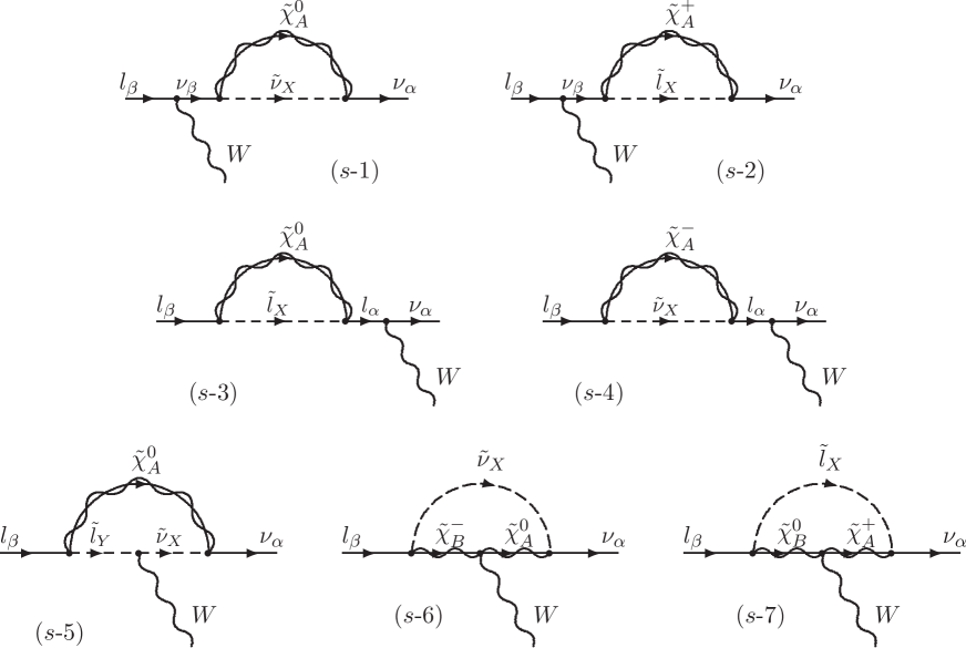
Figure 6: Diagrams which contribute to $(\epsilon^{s}_{\mu\tau})_{\text{$W$-penguin}}$.

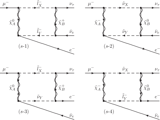
Figure 7: Diagrams which contribute to $(\epsilon^{s}_{\mu\tau})_{\text{box}}$.

The box-part is represented as

$$(\epsilon^{s}_{\mu\tau})_{\text{box}}=\sum_{i}\mathcal{B}^{(s\text{-}i)}_{\mu\tau},$$ (91)

and each contribution, which is shown in Fig. 7, is calculated to be

$$\mathcal{B}^{(s\text{-}1)}_{\beta\alpha}= \frac{1}{8\sqrt{2}G_{F}}J_{4}\left(M_{\tilde{\chi}^{0}_{A}},M_{\tilde{\chi}^{+}_{B}},m_{\tilde{l}_{X}},m_{\tilde{l}_{Y}}\right)(N_{R}^{(l)*})_{X}^{\beta A}(N_{R}^{(l)})_{eA}^{Y}(C_{R}^{(\nu)*})_{Y}^{eB}(C_{R}^{(\nu)})_{\alpha B}^{X},$$ (92)

$$\mathcal{B}^{(s\text{-}2)}_{\beta\alpha}= \frac{1}{8\sqrt{2}G_{F}}J_{4}\left(M_{\tilde{\chi}^{-}_{A}},M_{\tilde{\chi}^{0}_{B}},m_{\tilde{\nu}_{X}},m_{\tilde{\nu}_{Y}}\right)(C_{R}^{(l)*})^{\beta}_{AX}(C_{R}^{(l)})_{e}^{AY}(N_{R}^{(\nu)*})_{Y}^{eB}(N_{R}^{(\nu)})_{\alpha B}^{X},$$ (93)

$$\mathcal{B}^{(s\text{-}3)}_{\beta\alpha}= \frac{1}{4\sqrt{2}G_{F}}I_{4}\left(M_{\tilde{\chi}^{0}_{A}},M_{\tilde{\chi}^{+}_{B}},m_{\tilde{l}_{X}},m_{\tilde{\nu}_{Y}}\right)M_{\tilde{\chi}^{0}_{A}}M_{\tilde{\chi}^{+}_{B}}(N_{R}^{(l)*})_{X}^{\beta A}(N_{R}^{(\nu)*})_{Y}^{eA}(C_{R}^{(\nu)})^{X}_{\alpha B}(C_{R}^{(l)})_{e}^{BY},$$ (94)

$$\mathcal{B}^{(s\text{-}4)}_{\beta\alpha}= \frac{1}{4\sqrt{2}G_{F}}I_{4}\left(M_{\tilde{\chi}^{-}_{A}},M_{\tilde{\chi}^{0}_{B}},m_{\tilde{\nu}_{X}},m_{\tilde{l}_{Y}}\right)M_{\tilde{\chi}^{-}_{A}}M_{\tilde{\chi}^{0}_{B}}(C_{R}^{(l)*})^{\beta}_{AX}(C_{R}^{(\nu)*})_{X}^{eA}(N_{R}^{(\nu)})_{\alpha B}^{X}(N_{R}^{(l)})_{eB}^{Y},$$ (95)

where $I_{4}$ and $J_{4}$ are the functions which are given as

$$I_{4}(M_{A},M_{B},m_{X},m_{Y}) \equiv\int\frac{{\rm d}^{4}k}{(2\pi)^{4}{\rm i}}\frac{1}{(k^{2}-M_{A}^{2})(k^{2}-M_{B}^{2})(k^{2}-m_{X}^{2})(k^{2}-m_{Y}^{2})},$$ (96)

$$J_{4}(M_{A},M_{B},m_{X},m_{Y}) \equiv\int\frac{{\rm d}^{4}k}{(2\pi)^{4}{\rm i}}\frac{k^{2}}{(k^{2}-M_{A}^{2})(k^{2}-M_{B}^{2})(k^{2}-m_{X}^{2})(k^{2}-m_{Y}^{2})}.$$ (97)

B.2 For $\epsilon^{m}_{\mu\tau}$

Since the matter of the Earth is the neutral for $U(1)_{\text{em}}$, there is no contribution to $\epsilon^{m}_{\mu\tau}$ from photon-penguin diagrams. The $Z$-penguin contribution associated with a proton and that with a neutron cancel each other out. The contributions which need to be taken into account are the $Z$-penguin contribution associated with an electron and the box contributions:

$$\epsilon^{m,e}_{\mu\tau}=(\epsilon^{m,e}_{\mu\tau})_{\text{$Z$-penguin}}+(\epsilon^{m,e}_{\mu\tau})_{\text{box}},$$ (98)

$$\epsilon^{m,u}_{\mu\tau}=(\epsilon^{m,u}_{\mu\tau})_{\text{box}},$$ (99)

$$\epsilon^{m,d}_{\mu\tau}=(\epsilon^{m,d}_{\mu\tau})_{\text{box}}.$$ (100)

The penguin contribution consists of diagrams which are drawn in Fig. 8,

$$(\epsilon^{m,e}_{\mu\tau})_{\text{$Z$-penguin}}=\sum_{i}\mathcal{A}^{(m\text{-}i)}_{\mu\tau}.$$ (101)

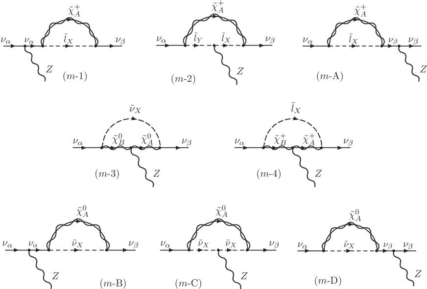
Figure 8: Diagrams which contributes to $(\epsilon^{m,e}_{\mu\tau})_{\text{$Z$-penguin}}$. The diagrams ($m$-A) and ($m$-D) are not counted into $\epsilon^{m}_{\mu\tau}$, which are included in $\epsilon^{s}_{\mu\tau}$ (cf. ($s$-2) and ($s$-1) in Fig. 6). The diagrams ($m$-B) and ($m$-C) cancel each other out after the off-shell prescription (Eq. (38)).

Each diagrams is calculated to be

$$\mathcal{A}^{(m\text{-}1)}_{\alpha\beta}= \frac{1}{(4\pi)^{2}}\frac{1}{2}\left(2\sin^{2}\theta_{W}-1\right)(C^{(\nu)}_{R})^{X}_{\beta A}(C^{(\nu)*}_{R})_{X}^{\alpha A}D(m_{\tilde{l}_{X}},M_{\tilde{\chi}^{+}_{A}}),$$ (102)

$$\mathcal{A}^{(m\text{-}2)}_{\alpha\beta}= -\frac{1}{(4\pi)^{2}}\left(2\sin^{2}\theta_{W}-1\right)(C^{(\nu)}_{R})^{X}_{\beta A}(C^{(\nu)*}_{R})^{\alpha A}_{Y}$$

$$\quad\times\left\{\left(-\frac{1}{2}+\sin^{2}\theta_{W}\right){(U_{\tilde{l}})_{X}}^{\gamma=\text{1-3}}{(U_{\tilde{l}}^{\dagger})_{\gamma=\text{1-3}}}^{Y}+\left(\sin^{2}\theta_{W}\right){(U_{\tilde{l}})_{X}}^{\gamma=\text{4-6}}{(U_{\tilde{l}}^{\dagger})_{\gamma=\text{4-6}}}^{Y}\right\}$$

$$\qquad\times E(m_{\tilde{l}_{X}},m_{\tilde{l}_{Y}},M_{\tilde{\chi}^{+}_{A}})$$ (103)

$$\mathcal{A}^{(m\text{-}3)}_{\alpha\beta}= -\frac{1}{(4\pi)^{2}}\left(2\sin^{2}\theta_{W}-1\right)(N^{(\nu)}_{R})^{X}_{\beta A}(N^{(\nu)*}_{R})^{\alpha B}_{X}$$

$$\quad\times\left[{(O^{\prime\prime L})_{A}}^{B}G\left(m_{\tilde{\nu}_{X}},M_{\tilde{\chi}^{0}_{A}},M_{\tilde{\chi}^{0}_{B}}\right)-\frac{1}{2}{(O^{\prime\prime R})^{A}}_{B}F\left(m_{\tilde{\nu}_{X}},M_{\tilde{\chi}^{0}_{A}},M_{\tilde{\chi}^{0}_{B}}\right)\right],$$ (104)

$$\mathcal{A}^{(m\text{-}4)}_{\alpha\beta}= -\frac{1}{(4\pi)^{2}}\left(2\sin^{2}\theta_{W}-1\right)(C^{(\nu)}_{R})^{X}_{\beta A}(C^{(\nu)*}_{R})^{\alpha B}_{X}$$

$$\quad\times\biggl{[}{(O^{\prime L})^{A}}_{B}G\left(m_{\tilde{l}_{X}},M_{\tilde{\chi}^{+}_{A}},M_{\tilde{\chi}^{+}_{B}}\right)-\frac{1}{2}{(O^{\prime R})^{A}}_{B}F\left(m_{\tilde{l}_{X}},M_{\tilde{\chi}^{+}_{A}},M_{\tilde{\chi}^{+}_{B}}\right)\biggr{]}.$$ (105)

The couplings for the chargino-chargino-$Z$-boson and neutralino-neutralino-$Z$-boson areHaberKane

$${(O^{\prime L})^{A}}_{B}= -{(U_{R}^{*})^{A}}_{1}{(U_{R})_{B}}^{1}-\frac{1}{2}{(U_{R}^{*})^{A}}_{2}{(U_{R})_{B}}^{2}+\delta^{A}_{B}\sin^{2}\theta_{W},$$ (106)

$${(O^{\prime R})^{A}}_{B}= -{(U_{L}^{*})^{A}}_{1}{(U_{L})_{B}}^{1}-\frac{1}{2}{(U_{L}^{*})^{A}}_{2}{(U_{L})_{B}}^{2}+\delta^{A}_{B}\sin^{2}\theta_{W},$$ (107)

$${(O^{\prime\prime L})_{A}}^{B}= -\frac{1}{2}{(U_{N})_{A}}^{3}{(U_{N}^{*})^{B}}_{3}+\frac{1}{2}{(U_{N})_{A}}^{4}{(U_{N}^{*})^{B}}_{4},$$ (108)

$${(O^{\prime\prime R})^{A}}_{B}= -{(O^{\prime\prime L*})^{A}}_{B}.$$ (109)

Here, we take into account the procedure to resolve the double counting problem which is explained in Sec. III.1.

The box contribution associated with the electron in the Earth’s matter is

$$(\epsilon^{m,e}_{\mu\tau})_{\text{box}}=\sum_{i}\mathcal{B}^{(m,e\text{-}i)}_{\mu\tau},$$ (110)

where

$$\mathcal{B}^{(m,e\text{-}1)}_{\alpha\beta}= \frac{1}{8\sqrt{2}G_{F}}J_{4}\left(M_{\tilde{\chi}^{0}_{A}},M_{\tilde{\chi}^{0}_{B}},m_{\tilde{\nu}_{X}},m_{\tilde{l}_{Y}}\right)(N^{(\nu)}_{R})^{X}_{\beta B}(N^{(l)*}_{R})^{eB}_{Y}(N^{(l)}_{R})^{Y}_{eA}(N^{(\nu)*}_{R})^{\alpha A}_{X},$$ (111)

$$\mathcal{B}^{(m,e\text{-}2)}_{\alpha\beta}= -\frac{1}{4\sqrt{2}G_{F}}I_{4}\left(M_{\tilde{\chi}^{0}_{A}},M_{\tilde{\chi}^{0}_{B}},m_{\tilde{\nu}_{X}},m_{\tilde{l}_{Y}}\right)M_{\tilde{\chi}^{0}_{A}}M_{\tilde{\chi}^{0}_{B}}(N^{(\nu)}_{R})^{X}_{\beta B}(N^{(l)*}_{L})^{e}_{BY}(N^{(l)}_{L})^{AY}_{e}(N^{(\nu)*}_{R})^{\alpha A}_{X},$$ (112)

$$\mathcal{B}^{(m,e\text{-}3)}_{\alpha\beta}= \frac{1}{4\sqrt{2}G_{F}}I_{4}\left(M_{\tilde{\chi}^{0}_{A}},M_{\tilde{\chi}^{0}_{B}},m_{\tilde{\nu}_{X}},m_{\tilde{l}_{Y}}\right)M_{\tilde{\chi}^{0}_{A}}M_{\tilde{\chi}^{0}_{B}}(N^{(\nu)}_{R})^{X}_{\beta B}(N^{(l)}_{R})^{Y}_{eB}(N^{(\nu)*}_{R})^{\alpha A}_{X}(N^{(l)*}_{R})^{eA}_{Y},$$ (113)

$$\mathcal{B}^{(m,e\text{-}4)}_{\alpha\beta}= -\frac{1}{8\sqrt{2}G_{F}}J_{4}\left(M_{\tilde{\chi}^{0}_{A}},M_{\tilde{\chi}^{0}_{B}},m_{\tilde{\nu}_{X}},m_{\tilde{l}_{Y}}\right)(N^{(\nu)}_{R})^{X}_{\beta B}(N^{(l)}_{R})^{Y}_{eB}(N^{(\nu)*}_{R})^{\alpha A}_{X}(N^{(l)*}_{R})^{eA}_{Y},$$ (114)

$$\mathcal{B}^{(m,e\text{-}5)}_{\alpha\beta}= \frac{1}{4\sqrt{2}G_{F}}I_{4}\left(M_{\tilde{\chi}^{+}_{A}},M_{\tilde{\chi}^{+}_{B}},m_{\tilde{l}_{X}},m_{\tilde{\nu}_{Y}}\right)M_{\tilde{\chi}^{+}_{A}}M_{\tilde{\chi}^{+}_{B}}(C^{(\nu)}_{R})^{X}_{\beta B}(C^{(l)}_{R})^{BY}_{e}(C^{(l)*}_{R})^{e}_{AY}(C^{(\nu)*}_{R})^{\alpha A}_{X},$$ (115)

$$\mathcal{B}^{(m,e\text{-}6)}_{\alpha\beta}= -\frac{1}{8\sqrt{2}G_{F}}J_{4}\left(M_{\tilde{\chi}^{+}_{A}},M_{\tilde{\chi}^{+}_{B}},m_{\tilde{l}_{X}},m_{\tilde{\nu}_{Y}}\right)(C^{(\nu)}_{R})^{X}_{\beta B}(C^{(l)}_{L})^{BY}_{e}(C^{(l)*}_{L})^{e}_{AY}(C^{(\nu)*}_{R})^{\alpha A}_{X},$$ (116)

$$\mathcal{B}^{(m,e\text{-}7)}_{\alpha\beta}= \frac{1}{4\sqrt{2}G_{F}}I_{4}\left(M_{\tilde{\chi}^{+}_{A}},M_{\tilde{\chi}^{0}_{B}},m_{\tilde{l}_{X}},m_{\tilde{\nu}_{Y}}\right)M_{\tilde{\chi}^{+}_{A}}M_{\tilde{\chi}^{0}_{B}}(N^{(l)}_{R})^{X}_{eB}(N^{(\nu)}_{R})^{Y}_{\beta B}(C^{(l)*}_{R})^{e}_{AY}(C^{(\nu)*}_{R})^{\alpha A}_{X},$$ (117)

$$\mathcal{B}^{(m,e\text{-}8)}_{\alpha\beta}= \frac{1}{8\sqrt{2}G_{F}}J_{4}\left(M_{\tilde{\chi}^{+}_{A}},M_{\tilde{\chi}^{0}_{B}},m_{\tilde{l}_{X}},m_{\tilde{\nu}_{Y}}\right)(N^{(l)}_{L})^{BX}_{e}(N^{(\nu)}_{R})^{Y}_{\beta B}(C^{(l)*}_{L})^{e}_{AY}(C^{(\nu)*}_{R})^{\alpha A}_{X},$$ (118)

$$\mathcal{B}^{(m,e\text{-}9)}_{\alpha\beta}= \frac{1}{4\sqrt{2}G_{F}}I_{4}\left(M_{\tilde{\chi}^{0}_{A}},M_{\tilde{\chi}^{-}_{B}},m_{\tilde{\nu}_{X}},m_{\tilde{l}_{Y}}\right)M_{\tilde{\chi}^{0}_{A}}M_{\tilde{\chi}^{-}_{B}}(C^{(l)}_{R})^{BX}_{e}(C^{(\nu)}_{R})^{Y}_{\beta B}(N^{(l)*}_{R})^{eA}_{Y}(N^{(\nu)*}_{R})^{\alpha A}_{X},$$ (119)

$$\mathcal{B}^{(m,e\text{-}10)}_{\alpha\beta}= \frac{1}{8\sqrt{2}G_{F}}J_{4}\left(M_{\tilde{\chi}^{0}_{A}},M_{\tilde{\chi}^{-}_{B}},m_{\tilde{\nu}_{X}},m_{\tilde{l}_{Y}}\right)(C^{(l)}_{L})^{BX}_{e}(C^{(\nu)}_{R})^{Y}_{\beta B}(N^{(l)*}_{L})^{eA}_{Y}(N^{(\nu)*}_{R})^{\alpha A}_{X}.$$ (120)

The box contribution associated with the down-quark in the matter of the Earth is

$$(\epsilon^{m,d}_{\mu\tau})_{\text{box}}=\sum_{i}\mathcal{B}^{(m,d\text{-}i)}_{\mu\tau},$$ (121)

where

$$\mathcal{B}^{(m,d\text{-}1)}_{\alpha\beta}= \frac{1}{8\sqrt{2}G_{F}}J_{4}\left(M_{\tilde{\chi}^{0}_{A}},M_{\tilde{\chi}^{0}_{B}},m_{\tilde{\nu}_{X}},m_{\tilde{d}_{Y}}\right)(N^{(\nu)}_{R})^{X}_{\beta B}(N^{(d)*}_{R})^{dB}_{Y}(N^{(d)}_{R})^{Y}_{dA}(N^{(\nu)*}_{R})^{\alpha A}_{X},$$ (122)

$$\mathcal{B}^{(m,d\text{-}2)}_{\alpha\beta}= -\frac{1}{4\sqrt{2}G_{F}}I_{4}\left(M_{\tilde{\chi}^{0}_{A}},M_{\tilde{\chi}^{0}_{B}},m_{\tilde{\nu}_{X}},m_{\tilde{d}_{Y}}\right)M_{\tilde{\chi}^{0}_{A}}M_{\tilde{\chi}^{0}_{B}}(N^{(\nu)}_{R})^{X}_{\beta B}(N^{(d)*}_{L})^{d}_{BY}(N^{(d)}_{L})^{AY}_{d}(N^{(\nu)*}_{R})^{\alpha A}_{X},$$ (123)

$$\mathcal{B}^{(m,d\text{-}3)}_{\alpha\beta}= \frac{1}{4\sqrt{2}G_{F}}I_{4}\left(M_{\tilde{\chi}^{0}_{A}},M_{\tilde{\chi}^{0}_{B}},m_{\tilde{\nu}_{X}},m_{\tilde{d}_{Y}}\right)M_{\tilde{\chi}^{0}_{A}}M_{\tilde{\chi}^{0}_{B}}(N^{(\nu)}_{R})^{X}_{\beta B}(N^{(d)}_{R})^{Y}_{dB}(N^{(\nu)*}_{R})^{\alpha A}_{X}(N^{(d)*}_{R})^{dA}_{Y},$$ (124)

$$\mathcal{B}^{(m,d\text{-}4)}_{\alpha\beta}= -\frac{1}{8\sqrt{2}G_{F}}J_{4}\left(M_{\tilde{\chi}^{0}_{A}},M_{\tilde{\chi}^{0}_{B}},m_{\tilde{\nu}_{X}},m_{\tilde{d}_{Y}}\right)(N^{(\nu)}_{R})^{X}_{\beta B}(N^{(d)}_{R})^{Y}_{dB}(N^{(\nu)*}_{R})^{\alpha A}_{X}(N^{(d)*}_{R})^{dA}_{Y},$$ (125)

$$\mathcal{B}^{(m,d\text{-}5)}_{\alpha\beta}= \frac{1}{4\sqrt{2}G_{F}}I_{4}\left(M_{\tilde{\chi}^{+}_{A}},M_{\tilde{\chi}^{+}_{B}},m_{\tilde{l}_{X}},m_{\tilde{u}_{Y}}\right)M_{\tilde{\chi}^{+}_{A}}M_{\tilde{\chi}^{+}_{B}}(C^{(\nu)}_{R})^{X}_{\beta B}(C^{(d)}_{R})^{BY}_{d}(C^{(d)*}_{R})^{d}_{AY}(C^{(\nu)*}_{R})^{\alpha A}_{X},$$ (126)

$$\mathcal{B}^{(m,d\text{-}6)}_{\alpha\beta}= -\frac{1}{8\sqrt{2}G_{F}}J_{4}\left(M_{\tilde{\chi}^{+}_{A}},M_{\tilde{\chi}^{+}_{B}},m_{\tilde{l}_{X}},m_{\tilde{u}_{Y}}\right)(C^{(\nu)}_{R})^{X}_{\beta B}(C^{(d)}_{L})^{BY}_{d}(C^{(d)*}_{L})^{d}_{AY}(C^{(\nu)*}_{R})^{\alpha A}_{X}.$$ (127)

The box contribution associated with the up-quark in the matter of the Earth is

$$(\epsilon^{m,u}_{\mu\tau})_{\text{box}}=\sum_{i}\mathcal{B}^{(m,u\text{-}i)}_{\mu\tau},$$ (128)

where

$$\mathcal{B}^{(m,u\text{-}1)}_{\alpha\beta}= \frac{1}{8\sqrt{2}G_{F}}J_{4}\left(M_{\tilde{\chi}^{0}_{A}},M_{\tilde{\chi}^{0}_{B}},m_{\tilde{\nu}_{X}},m_{\tilde{u}_{Y}}\right)(N^{(\nu)}_{R})^{X}_{\beta B}(N^{(u)*}_{R})^{uB}_{Y}(N^{(u)}_{R})^{Y}_{uA}(N^{(\nu)*}_{R})^{\alpha A}_{X},$$ (129)

$$\mathcal{B}^{(m,u\text{-}2)}_{\alpha\beta}= -\frac{1}{4\sqrt{2}G_{F}}I_{4}\left(M_{\tilde{\chi}^{0}_{A}},M_{\tilde{\chi}^{0}_{B}},m_{\tilde{\nu}_{X}},m_{\tilde{u}_{Y}}\right)M_{\tilde{\chi}^{0}_{A}}M_{\tilde{\chi}^{0}_{B}}(N^{(\nu)}_{R})^{X}_{\beta B}(N^{(u)*}_{L})^{u}_{BY}(N^{(u)}_{L})^{AY}_{u}(N^{(\nu)*}_{R})^{\alpha A}_{X},$$ (130)

$$\mathcal{B}^{(m,u\text{-}3)}_{\alpha\beta}= \frac{1}{4\sqrt{2}G_{F}}I_{4}\left(M_{\tilde{\chi}^{0}_{A}},M_{\tilde{\chi}^{0}_{B}},m_{\tilde{\nu}_{X}},m_{\tilde{u}_{Y}}\right)M_{\tilde{\chi}^{0}_{A}}M_{\tilde{\chi}^{0}_{B}}(N^{(\nu)}_{R})^{X}_{\beta B}(N^{(u)}_{R})^{Y}_{uB}(N^{(\nu)*}_{R})^{\alpha A}_{X}(N^{(u)*}_{R})^{uA}_{Y},$$ (131)

$$\mathcal{B}^{(m,u\text{-}4)}_{\alpha\beta}= -\frac{1}{8\sqrt{2}G_{F}}J_{4}\left(M_{\tilde{\chi}^{0}_{A}},M_{\tilde{\chi}^{0}_{B}},m_{\tilde{\nu}_{X}},m_{\tilde{u}_{Y}}\right)(N^{(\nu)}_{R})^{X}_{\beta B}(N^{(u)}_{R})^{Y}_{uB}(N^{(\nu)*}_{R})^{\alpha A}_{X}(N^{(u)*}_{R})^{uA}_{Y},$$ (132)

$$\mathcal{B}^{(m,u\text{-}5)}_{\alpha\beta}= \frac{1}{8\sqrt{2}G_{F}}J_{4}\left(M_{\tilde{\chi}^{+}_{A}},M_{\tilde{\chi}^{+}_{B}},m_{\tilde{l}_{X}},m_{\tilde{d}_{Y}}\right)(C^{(\nu)}_{R})^{X}_{\beta B}(C^{(u)*}_{R})^{uB}_{Y}(C^{(u)}_{R})^{Y}_{uA}(C^{(\nu)*}_{R})^{\alpha A}_{X},$$ (133)

$$\mathcal{B}^{(m,u\text{-}6)}_{\alpha\beta}= -\frac{1}{4\sqrt{2}G_{F}}I_{4}\left(M_{\tilde{\chi}^{+}_{A}},M_{\tilde{\chi}^{+}_{B}},m_{\tilde{l}_{X}},m_{\tilde{d}_{Y}}\right)M_{\tilde{\chi}^{+}_{A}}M_{\tilde{\chi}^{+}_{B}}(C^{(\nu)}_{R})^{X}_{\beta B}(C^{(u)*}_{L})^{uB}_{Y}(C^{(u)}_{L})^{Y}_{uA}(C^{(\nu)*}_{R})^{\alpha A}_{X}.$$ (134)

B.3 For $\epsilon^{d}_{\mu\tau}$

We consider the charged current interaction between neutrino beam and the nucleon in the detector as a detection process. It consists of the penguin contribution and the box contribution;

$$\epsilon^{d}_{\mu\tau}=(\epsilon^{d}_{\mu\tau})_{\text{$W$-penguin}}+(\epsilon^{d}_{\mu\tau})_{\text{box}}.$$ (135)

The penguin contribution can be represented as the complex conjugate of that for $\epsilon^{s}_{\tau\mu}$. However, we must eliminate the diagrams which are already counted in the calculation of $\epsilon^{m}_{\mu\tau}$. The detail is shown in Sec. III.1.

$$(\epsilon^{d}_{\mu\tau})_{\text{$W$-penguin}}=\sum_{i=3}^{7}\mathcal{A}^{(s\text{-}i)*}_{\tau\mu}.$$ (136)

The box contribution is calculated to be

$$(\epsilon^{d}_{\mu\tau})_{\text{box}}=\sum_{i}\mathcal{B}^{(d\text{-}i)}_{\mu\tau},$$ (137)

where

$$\mathcal{B}^{(d\text{-}1)}_{\alpha\beta}= \frac{1}{8\sqrt{2}G_{F}}J_{4}\left(M_{\tilde{\chi}^{0}_{A}},M_{\tilde{\chi}^{-}_{B}},m_{\tilde{\nu}_{X}},m_{\tilde{u}_{Y}}\right)(C^{(l)}_{R})^{BX}_{\beta}(C^{(d)*}_{R})^{d}_{BY}(N_{R}^{(u)})^{Y}_{uA}(N^{(\nu)*})^{\alpha A}_{X},$$ (138)

$$\mathcal{B}^{(d\text{-}2)}_{\alpha\beta}= \frac{1}{8\sqrt{2}G_{F}}J_{4}\left(M_{\tilde{\chi}^{+}_{A}},M_{\tilde{\chi}^{0}_{B}},m_{\tilde{l}_{X}},m_{\tilde{d}_{Y}}\right)(N^{(l)}_{R})^{X}_{\beta B}(N^{(d)*}_{R})^{dB}_{Y}(C^{(u)}_{R})^{Y}_{uA}(C^{(\nu)*}_{R})^{\alpha A}_{X},$$ (139)

$$\mathcal{B}^{(d\text{-}3)}_{\alpha\beta}= \frac{1}{4\sqrt{2}G_{F}}I_{4}\left(M_{\tilde{\chi}^{0}_{A}},M_{\tilde{\chi}^{+}_{B}},m_{\tilde{\nu}_{X}},m_{\tilde{d}_{Y}}\right)M_{\tilde{\chi}^{0}_{A}}M_{\tilde{\chi}^{+}_{B}}(C^{(l)}_{R})^{BX}_{\beta}(C^{(u)}_{R})^{Y}_{uB}(N^{(d)*}_{R})^{dA}_{Y}(N^{(\nu)}_{R})^{\alpha A}_{X},$$ (140)

$$\mathcal{B}^{(d\text{-}4)}_{\alpha\beta}= \frac{1}{4\sqrt{2}G_{F}}I_{4}\left(M_{\tilde{\chi}^{-}_{A}},M_{\tilde{\chi}^{0}_{B}},m_{\tilde{l}_{X}},m_{\tilde{u}_{Y}}\right)M_{\tilde{\chi}^{-}_{A}}M_{\tilde{\chi}^{0}_{B}}(N^{(l)}_{R})^{X}_{\beta B}(N^{(u)}_{R})^{Y}_{uB}(C_{R}^{(d)*})^{d}_{AY}(C^{(\nu)*}_{R})^{\alpha A}_{X}.$$ (141)

References

- (1) B. T. Cleveland et al., Astrophys. J. 496 (1998) 505.
- (2) SAGE Collaboration, J. N. Abdurashitov et al., J. Exp. Theor. Phys. 95 (2002) 181 [Zh. Eksp. Teor. Fiz. 122 (2002) 211].
- (3) GALLEX Collaboration, W. Hampel et al., Phys. Lett. B447 (1999) 127.
- (4) GNO Collaboration, M. Altmann et al., Phys. Lett. B490 (2000) 16.
- (5) Super-Kamiokande Collaboration, M. Smy et al., Phys. Rev. D69 (2004) 011104; S. Fukuda et al., Phys. Rev. Lett. 86 (2001) 5651; ibid. 86 (2001) 5656; Phys. Lett. B539 (2002) 179.
- (6) SNO Collaboration, S. N. Ahmed et al., Phys. Rev. Lett. 92 (2004) 181301; Q. R. Ahmad et al., Phys. Rev. Lett. 87 (2001) 071301; ibid. 89 (2002) 011301; ibid. 89 (2002) 011302.
- (7) Super-Kamiokande Collaboration, Y. Ashie et al., arXiv:hep-ex/0501064; Phys. Rev. Lett. 93 (2004) 101801; Y. Fukuda et al., Phys. Rev. Lett. 81 (1998) 1562; ibid. 82 (1999) 2644; ibid. 82 (1999) 5194.
- (8) G. Giacomelli and A. Margiotta, Phys. Atom. Nucl. 67 (2004) 1139 [Yad. Fiz. 67 (2004) 1165].
- (9) Soudan 2 Collaboration, M. Sanchez et al., Phys. Rev. D68 (2003) 113004.
- (10) KamLAND Collaboration, T. Araki et al., arXiv:hep-ex/0406035; K. Eguchi et al., Phys. Rev. Lett. 90 (2003) 021802.
- (11) K2K Collaboration, M. H. Ahn et al., Phys. Rev. Lett. 90 (2003) 041801.
-
(12)
P. Minkowski, Phys. Lett. B67 (1977) 421.
T. Yanagida, in Proceedings of the Workshop on Unified Theory and Baryon Number of the Universe, edited by O. Sawada and A. Sugamoto, Report KEK-79-18 (1979).
M. Gell-Mann, P. Ramond and R. Slansky, in Supergravity, edited by D. Z. Freedman and P. van Nieuwenhuizen (North-Holland, Amsterdam, 1979). - (13) F. Borzumati and A. Masiero, Phys. Rev. Lett. 57 (1986) 961.
- (14) J. Hisano, T. Moroi, K. Tobe, M. Yamaguchi and T. Yanagida, Phys. Lett. B357 (1995) 579; J. Hisano, T. Moroi, K. Tobe and M. Yamaguchi, Phys. Rev. D53 (1996) 2442.
- (15) See e.g., J. Hisano and D. Nomura, Phys. Rev. D59 (1999) 116005; W. Buchmüller, D. Delphine and F. Vissani, Phys. Lett. B459 (1999) 171; W. Buchmüller, D. Delphine and L. T. Handoko, Nucl. Phys. B576 (2000) 445; J. Ellis, M. E. Gomez, G. K. Leontaris, S. Lola and D. V. Nanopoulos, Eur. Phys. J. C14 (2000) 319; S. Baek, T. Goto, Y. Okada and K. Okumura, Phys. Rev. D63 (2001) 051701; J. Sato and K. Tobe, Phys. Rev. D63(2001) 116010; J. Sato, K. Tobe and T. Yanagida, Phys. Lett. B498 (2001) 189; J. A. Casas and A. Ibarra, Nucl. Phys. B618 (2001) 171; S. Davidson and A. Ibarra, JHEP 0109 (2001) 013; S. Lavignac, I. Masina and C. A. Savoy, Phys. Lett. B520 (2001) 269; J. Hisano and K. Tobe, Phys. Lett. B510 (2001) 197; J. Ellis and M. Raidal, Nucl. Phys. B643 (2002) 229; T. Blazek and S. F. King, Nucl. Phys. B 662 (2003) 359; S. Pascoli, S. T. Petcov and C. E. Yaguna, Phys. Lett. B564 (2003) 241; S. Pascoli, S. T. Petcov and W. Rodejohann, Phys. Rev. D68 (2003) 093007; A. Masiero, S. Profumo, S. K. Vempati and C. E. Yaguna, JHEP 0403 (2004) 046; A. Masiero, S. K. Vempati and O. Vives, New J. Phys. 6 (2004) 202; S. T. Petcov, S. Profumo, Y. Takanishi and C. E. Yaguna, Nucl. Phys. B676 (2004) 453; I. Masina and C. A. Savoy, arXiv:hep-ph/0501166; S. Kanemura, K. Matsuda, T. Ota, T. Shindou, E. Takasugi and K. Tsumura, arXiv:hep-ph/0501228.
-
(16)
L.M. Barkov et al., Research Proposal to PSI, 1999,
See the webpage:
http://www.icepp.s.u-tokyo.ac.jp/meg. -
(17)
MECO Collaboration, M. Bachman et al.,
Proposal to BNL, 1997.
See the webpage:
http://meco.ps.uci.edu. -
(18)
For example, see technical notes in the webpage of the PRISM project,
http://psux1.kek.jp/~prism.
See also the webpage of Neutrino factory and muon storage rings at CERN,
http://muonstoragerings.web.cern.ch/muonstoragerings/. - (19) JHF-Kamioka project, Y. Itow et al., arXiv:hep-ex/0106019.
- (20) Neutrino Factory and Muon Collider Collaboration, C. Albright et al., arXiv:physics/0411123; C. Albright et al., arXiv:hep-ex/0008064; Neutrino Factory and Muon Collider Collabollation, D. Ayres et al., arXiv:physics/9911009; D. Harris, et al., eConf C010630 (2001) E1001 [arXiv:hep-ph/0111030].
- (21) P. Huber, M. Lindner, M. Rolinec, T. Schwetz and W. Winter, Phys. Rev. D70 (2004) 073014.
- (22) Y. Grossman, Phys. Lett. B359 (1995) 141.
- (23) M. C. Gonzalez-Garcia, Y. Grossman, A. Gusso and Y. Nir, Phys. Rev. D64 (2001) 096006.
- (24) A. M. Gago, M. M. Guzzo, H. Nunokawa, W. J. C. Teves and R. Zukanovich Funchal, Phys. Rev. D64 (2001) 073003.
- (25) P. Huber and J. W. F. Valle, Phys. Lett. B523 (2001) 151.
- (26) T. Ota, J. Sato and N. Yamashita, Phys. Rev. D65 (2002) 093015.
- (27) T. Ota and J. Sato, Phys. Lett. B545 (2002) 367.
- (28) P. Huber, T, Schwetz and J. W. F. Valle, Phys. Rev. D66 (2002) 013006.
- (29) M. Campanelli and A. Romanino, Phys. Rev. D66 (2002) 113001.
- (30) T. Hattori, T. Hasuike and S. Wakaizumi, arXiv:hep-ph/0210138.
- (31) M. Garbutt and B. H. J. McKellar, arXiv:hep-ph/0308111.
- (32) S. Davidson, C. Pena-Garay, N. Rius and A. Santamaria, JHEP 0303 (2003) 011.
- (33) See e.g., E. Roulet, Phys. Rev. D44 (1991) 935; M. M. Guzzo, A. Masiero and S. T. Petcov, Phys. Lett. B260 (1991) 154; M. M. Guzzo and S. T. Petcov, Phys. Lett. B271 (1991) 172; V. D. Barger, R. J. N. Phillips and K. Whisnant, Phys. Rev. D44 (1991) 1629; S. Degl’Innocenti and B. Ricci, Mod. Phys. Lett. A8 (1993) 471; G. L. Fogli and E. Lisi, Astropart. Phys. 2 (1994) 91; P. I. Krastev and J. N. Bahcall, Proceedings of Flavor Changing Neutral Currents: Present and Future Studies (FCNC 97), edited by D. B. Cline, (World Scientific, Singapore, 1997) p.259 [arXiv:hep-ph/9703267]; E. Ma and P. Roy, Phys. Rev. Lett. 80 (1998) 4637; S. Bergmann, Nucl. Phys. B515 (1998) 363; S. Bergmann and A. Kagan, Nucl. Phys. B538 (1999) 368; S. Bergmann, M. M. Guzzo, P. C. de Holanda, P. I. Krastev and H. Nunokawa, Phys. Rev. D62 (2000) 073001; A. M. Gago, M. M. Guzzo, P. C. de Holanda, H. Nunokawa, O. L. G. Peres, V. Pleitez and R. Zukanovich Funchal, Phys. Rev. D65 (2002) 073012; M. Guzzo, P. C. de Holanda, M. Maltoni, H. Nunokawa, M. A. Tortola and J. W. F. Valle, Nucl. Phys. B629 (2002) 479; Z. Berezhiani, R. S. Raghavan, A. Rossi, Nucl. Phys. B638 (2002) 62; A. Friedland, C. Lunardini and C. Pena-Garay, Phys. Lett. B594 (2004) 347; M. M. Guzzo, P. C. de Holanda and O. L. G. Peres, Phys. Lett. B591 (2004) 1; O. G. Miranda, M. A. Tórtola and J. W. F. Valle, arXiv:hep-ph/0406280.
- (34) See e.g, P. Lipari and M. Lusignoli, Phys. Rev. D60 (1999) 013003; G. L. Fogli, E. Lisi, A. Marrone and G. Scioscia, Phys. Rev. D60 (1999) 053006; N. Fornengo, M. Maltoni, R. T. Bayo and J. W. F. Valle, Phys. Rev. D65 (2002) 013010; A. Friedland, C. Lunardini and M. Maltoni, Phys. Rev. D70 (2004) 111301; M. C. Gonzalez-Garcia and M. Maltoni, Phys. Rev. D70 (2004) 033010.
- (35) S. Bergmann and Y. Grossman, Phys. Rev. D59 (1999) 093005.
- (36) See e.g., J. W. F. Valle, Phys. Lett. B199 (1987) 432; H. Nunokawa, Y. Z. Qian, A. Rossi and J. W. F. Valle, Phys. Rev. D54 (1996) 4356; H. Nunokawa, A. Rossi and J. W. F. Valle, Nucl. Phys. B482 (1996) 481; S. Mansour and T. K. Kuo, Phys. Rev. D58 (1998) 013012; G. L. Fogli, E. Lisi, A. Mirizzi and D. Montanino, Phys. Rev. D66 (2002) 013009.
- (37) G. C. Branco, D. Delepine, B. Nobre, and J. Santiago, Nucl. Phys. B657 (2003) 355; A. Datta, R. Gandhi, B. Mukhopadhyaya and Poonam Mehta, Phys. Rev. D64 (2001) 015011; L. M. Johnson and D. W. McKay, Phys. Lett. B433 (1998) 355.
- (38) C. Giunti, arXiv:hep-ph/0409230.
- (39) B. Kayser, Phys. Rev. D24 (1981) 110; C. Giunti, C. W. Kim and U. W. Lee, Phys. Rev. D44 (1991) 3635.
- (40) S. Bergmann, Y. Grossman and E. Nardi, Phys. Rev. D60 (1999) 093008.
- (41) T. Ota and J. Sato, arXiv:hep-ph/0410408.
- (42) Belle Collaboration, K. Abe et al., Phys. Rev. Lett. 92 (2004) 171802.
- (43) M. Fukugita and T. Yanagida, “Physics of Neutrinos and applications to Astrophysics”, (Springer-Verlag, Germany, 2003).
- (44) K. Inoue, A. Kakuto, H. Komatsu and S. Takeshita, Prog. Theor. Phys. 68 (1982) 927.
- (45) H. Haber and G. Kane, Phys. Rept. 117 (1985) 75.