OPE coefficient functions in terms of composite operators only. Nonsinglet case

Abstract

A new method for calculating the coefficient functions of the operator product expansion is proposed which does not depend explicitly on elementary fields. Coefficient functions are defined entirely in terms of composite operators. The method is illustrated in the case of QCD nonsinglet operators.

PACS numbers: 11.10.-z, 11.10.Gh, 12.38.-t

1 Introduction

The structure functions of deep inelastic lepton-proton scattering (DIS) are related with an absorptive part of the matrix elements

$$i\int\!d^{4}x\,\mbox{e}^{iqx}\langle\,p\,|\mathrm{T}J^{em}_{\mu}(x)J^{em}_{\nu}(0)|\,p\,\rangle.$$ (1)

Here $J^{em}_{\mu}(x)$ is an electromagnetic current and $|\,p\,\rangle$ means a proton state. In its turn, an expansion of a chronological product of two electromagnetic currents near the light-cone in terms of composite operators $O^{a,\,m}$ looks like:

$$\mbox{T}J^{em}_{\mu}(x)J^{em}_{\nu}(0)=-g_{\mu\nu}\sum\limits_{a}\sum\limits_{\mathrm{even}\,m}C^{(1)}_{a,\,m}(x^{2},\mu^{2})\,\frac{i^{m}}{m!}\,x^{\mu_{1}}\ldots x^{\mu_{m}}\,O^{a,\,m}_{\mu_{1}\ldots\mu_{m}}(0;\mu^{2})$$

$$+\sum\limits_{a}\sum\limits_{\mathrm{even}\,m}C^{(2)}_{a,\,m}(x^{2},\mu^{2})\,\frac{i^{m}}{m!}\,x^{\mu_{1}}\ldots x^{\mu_{m}}\,O^{a,\,m}_{\mu\nu\mu_{1}\ldots\mu_{m}}(0;\mu^{2})+\ldots\ ,$$ (2)

where $a=$ NS, S, $g$. The dots denote other Lorentz structure, constant term as well as gradient terms. The latter give no contribution to DIS structure functions. The index $a$ runs all allowed types of the composite operators. The expansion (1) is a generalization of the operator product expansion (OPE) at small distances [1]. It is known as light-cone OPE [2] (see also [3, 4]). The quantity $C^{(i)}_{a,\,m}$ is called an OPE coefficient function (CF). The composite operators in Eq. (1) need a regularization. After a renormalization of the operators, there arises a dependence of CF’s on a renormalization scale $\mu$.

On the other hand, the DIS structure functions can be represented in a factorizable form [5]. For instance, we have

$$\frac{1}{x}\,F_{2}(x,Q^{2})=\sum_{a}\int\limits_{x}^{1}\frac{dz}{z}\,C_{a}\!\left(\!z,\frac{Q^{2}}{M^{2}}\right)\,f_{a}\!\left(\frac{x}{z},M^{2}\right).$$ (3)

Here $f_{a}(x,M^{2})$ is a distribution of a parton of type $a$ inside the nucleon, while quantities $C_{a}(x,Q^{2}/M^{2})$ are known as DIS coefficient functions. In Eq. (3), $M$ is a factorization scale. It is usually identified with the renormalization scale $\mu$. The $m$-th moment of the DIS coefficient function, $C_{a}(m,Q^{2}/\mu^{2})$, is identified with the Fourier transform of the corresponding OPE CF’s in (1). The parton distributions $f_{a}(x,\mu^{2})$ are related with matrix elements of the composite operators between one-nucleon states (for details, see [3]).

The coefficient functions $C_{a}(x,Q^{2}/M^{2})$ were calculated in perturbative QCD. For example, contributions of the first and second orders in $\alpha_{s}$ can be found in Refs. [6] (where light quarks were considered), and in Refs. [7] (where both light and heavy quarks were accounted for). Note that a very definition of DIS coefficient functions applies to the diagram (perturbative) technique, not to the operator formalism. Moreover, since nucleon wave function is yet unknown, one has to deal with diagrams which describe a lepton scattering off (nonphysical) quark or gluon off-shell state.

The light-cone OPE for the scalar theory was studied in Refs. [8] in which rules for calculating CF’s were presented. Note that the T-product of two scalar currents near the light-cone was defined in term of so-called bi-local light-ray composite fields [8]. The local light-cone expansion can be obtained by performing a Taylor expansion of the non-local one [9]. The non-local expansion is more general, but we restrict ourselves to considering local OPE. In Refs. [10] a problem of finding $n$-loop contributions to the OPE CF’s were reduced to evaluating of propagator type $(n+1)$-loop Feynman diagrams.

The goal of the present paper is to present a derivation of a closed representation for the OPE CF’s in term of composite operator Green functions which does not lean on the perturbation theory. This will be done in the next Section. In Section 3 we check a validity of our results in a free scalar field theory. In Section 4 we calculate nonsinglet CF’s in perturbative QCD in order to demonstrate that our main formulae not only reproduces well-known expressions for the quark CF’s, but enables us to obtain CF’s of the gradient operators in the OPE. The finite renormalization of CF’s is considered in Section 5. In Appendix A a number of useful mathematical formulae is collected. In Appendix B we show that our scheme does result in a set of homogeneous renormalization group equations for the OPE CF’s.

2 OPE coefficient functions and matrix
elements of composite operators

Let us define a quark electromagnetic current

$$J^{em}_{\mu}(x)=\overline{\Psi}(x)\gamma_{\mu}Q\Psi(x),$$ (4)

where $\Psi(x)$ is a quark field. The electric charge operator in (4),

$$Q=\frac{1}{2}(\lambda^{3}+\frac{1}{\sqrt{3}}\lambda^{8}),$$ (5)

obeys the equations:

$$Q^{2}=\frac{1}{6}\left(\lambda^{3}+\frac{1}{\sqrt{3}}\lambda^{8}+\frac{4}{3}\lambda^{0}\right),$$ (6)

$$\mbox{Sp}(Q^{2}\lambda^{a})=\frac{1}{3}\left(\delta_{a3}+\frac{1}{\sqrt{3}}\delta_{a8}+2\,\delta_{a0}\right).$$ (7)

Here $\lambda^{a}$ ($a=1,2,\ldots 8$) are the Gell-Mann matrices, $\mbox{Sp}(\lambda^{a}\lambda^{b})=2\delta_{ab}$, and $\lambda^{0}$ is the identity matrix.

The operator product expansion (OPE) for the $\mathrm{T}$-product of two electromagnetic currents looks like (see, for instance, [4])

$$\mbox{T}J^{em}_{\mu}(x)J^{em}_{\nu}(0) = -\frac{1}{6}\,g_{\mu\nu}\sum\limits_{m=0}^{\infty}\sum\limits_{l=1}^{m}C_{1,\,NS}^{m,l}(x^{2})\,\frac{i^{m}}{m!}\,x^{\mu_{1}}\ldots x^{\mu_{m}}$$ (8)

$$\times \left[O^{3,\,m,l}_{NS,\,\mu_{1}\ldots\mu_{m}}(0)+\frac{1}{\sqrt{3}}O^{8,\,m,l}_{NS,\,\mu_{1}\ldots\mu_{m}}(0)\right]+\ldots\ ,$$

where the dots denote contributions from other Lorentz structures and singlet quark and gluon operators. It is clear from (7) that this expansion should contain nonsinglet (triplet and octet) and singlet composite operators.

Near the light-cone, a leading contribution comes from twist-2 operators. For instance, quark twist-2 (traceless) operator is of the form (operator $\mathbf{S}$ means a complete symmetrization in Lorentz indices):

$$O^{a,\,m,l}_{NS,\,\mu_{1}\ldots\mu_{m}}(x) = i^{m-1}\mathbf{S}\,\partial_{\mu_{l+1}}\ldots\partial_{\mu_{m}}\overline{\Psi}(x)\gamma_{\mu_{1}}D_{\mu_{2}}\ldots D_{\mu_{l}}\lambda^{a}\Psi(x)$$ (9)

$$+ (\mbox{terms proportional to }g_{\mu_{i}\mu_{j}}).$$

Here

$$D_{\mu}=\partial_{\mu}+ig\,t_{a}A^{a}_{\mu}\qquad(t^{a}=\lambda^{a}/2)$$ (10)

is a covariant derivative, and $A^{a}_{\mu}(x)$ is a gluon field.

If the OPE (8) is applied to deep inelastic scattering, only operators of the type

$$O^{a,\,m}_{NS,\,\mu_{1}\ldots\mu_{m}}(x) = i^{m-1}\mathbf{S}\,\overline{\Psi}(x)\gamma_{\mu_{1}}D_{\mu_{2}}\ldots D_{\mu_{m}}\lambda^{a}\Psi(x)$$ (11)

$$+ (\mbox{terms proportional to }g_{\mu_{i}\mu_{j}})$$

are important, since forward matrix elements of the operators with $1\leqslant l\leqslant m-1$ are zero. For non-forward Compton scattering, all operators contribute proportionally to $(p-p^{\prime})_{\mu_{l+1}}\ldots(p-p^{\prime})_{\mu_{m}}$. The invariant structure which survives at $p^{\prime}\rightarrow p$ can be related to the “skew” parton distributions. In our notation, $O^{a,\,m}_{NS,\,\mu_{1}\ldots\mu_{m}}=O^{a,\,m,m}_{NS,\,\mu_{1}\ldots\mu_{m}}$.

In general case, all operators with $1\leqslant l\leqslant m$ should be take into account, since they are mixed under the renormalization, and a renormalized operator $O^{m,l}_{\mathrm{R}}$ is defined via unrenormalized operators $O^{m,l}_{\mathrm{U}}$ by the relation (we have dropped non-relevant indices):

$$O^{m,l}_{\mathrm{U}}=\sum_{l^{\prime}=1}^{l}Z^{l}_{l^{\prime}}\,O^{m,l^{\prime}}_{\mathrm{R}},$$ (12)

where $\mathbf{Z}$ is a triangle matrix. In particular, we find that the composite operator $O^{m,1}$ is multiplicatively renormalized, while the composite operator $O^{m,m}$, which is relevant to DIS, is not. In perturbative QCD in the first order of $\alpha_{s}=g^{2}/(4\pi)$, elements of the matrix $\mathbf{Z}$ are given by the following expressions [4] (with non-significant finite terms omitted):

$$Z_{ll^{\prime}}=\left\{\begin{array}[]{cl}\displaystyle 1+C_{F}\,\frac{\alpha_{s}}{4\pi}\,\left[\frac{1}{\varepsilon}+\ln\left(\frac{\bar{\mu}^{2}}{\mu^{2}}\right)\right]\Big{[}-4\sum\limits_{j=2}^{l}\frac{1}{j}-1+\frac{2}{l(l+1)}\Big{]},&l^{\prime}=l,\\ \displaystyle C_{F}\,\frac{\alpha_{s}}{2\pi}\,\left[\frac{1}{\varepsilon}+\ln\left(\frac{\bar{\mu}^{2}}{\mu^{2}}\right)\right]\Big{[}\frac{1}{l-l^{\prime}}-\frac{1}{l+1}\Big{]},&l^{\prime}<l,\\ 0,&l^{\prime}>l,\\ \end{array}\right.$$ (13)

where $C_{F}=(N_{c}-1)/2N_{c}$, with $N_{c}$ being a number of colors. In deriving (13), a dimensional regularization [11] was used, and $\varepsilon=2-D/2$, where $D$ is the number of dimensions. Here and below $\bar{\mu}$ denotes the regularization mass, while $\mu$ denotes the renormalization scale.

In what follows, we will be interested in one of nonsinglet quark operators, namely, in $O^{3,\,m,l}_{NS,\,\mu_{1}\ldots\mu_{m}}(x)$. Let us introduce brief notations:

$$O^{m,l}_{\mu_{1}\ldots\mu_{m}}(x) \equiv O^{3,\,m,l}_{NS,\,\mu_{1}\ldots\mu_{m}}(x),$$ (14)

$$C_{m,l}(x^{2}) \equiv C_{1,\,NS}^{m,l}(x^{2}).$$ (15)

After multiplying both sides of Eq. (8) by the operator $O^{n,k}_{\nu_{1}\ldots\nu_{n}}$ (with arbitrary $n$, and $k=1,2\ldots n$), we get the following relation for $\mathrm{T}$-products of the composite operators between the vacuum states:

$$\int\!d^{4}x\,\mbox{e}^{iqx}\int\!d^{4}z\,\mbox{e}^{ipz}\langle\mathrm{T}J^{em}_{\mu}(x)J^{em}_{\nu}(0)\,O^{n,k}_{\nu_{1}\ldots\nu_{n}}(z)\rangle$$

$$=-\frac{1}{6}\,g_{\mu\nu}\sum\limits_{m=0}^{\infty}\sum\limits_{l=1}^{m}\frac{i^{m}}{m!}\,\int\!d^{4}x\,\mbox{e}^{iqx}\,C_{m,l}(x^{2})\,x_{\mu_{1}}\ldots x_{\mu_{m}}$$

$$\times\int\!d^{4}z\,\mbox{e}^{ipz}\langle\mbox{T}O^{m,l}_{\mu_{1}\ldots\mu_{m}}(0)\,O^{n,k}_{\nu_{1}\ldots\nu_{n}}(z)\rangle+\ldots\ .$$ (16)

Here dots mean other Lorentz structures. It is necessary to stress that propagator of only singlet quark operator has to appeared in (2), due to relation (7).

As usual, we assume that $C_{m,l}(x^{2})$ are tempered generalized functions (this is explicit in perturbative calculations) so the symbolic relation

$$x^{\mu_{1}}\ldots x^{\mu_{m}}=(-2i)^{m}\,\frac{q^{\mu_{1}}\ldots q^{\mu_{m}}}{(-q^{2})^{m}}\,(-q^{2})^{m}\left(\frac{\partial}{\partial q^{2}}\right)^{m}$$ (17)

holds in connection with the Fourier transform in (2). Then we obtain that

$$\int\!d^{4}x\,\mbox{e}^{iqx}\int\!d^{4}z\,\mbox{e}^{ipz}\langle\mbox{T}J^{em}_{\mu}(x)J^{em}_{\nu}(0)\,O^{n,k}_{\nu_{1}\ldots\nu_{n}}(z)\rangle$$

$$=-g_{\mu\nu}\sum\limits_{m=0}^{\infty}\sum\limits_{l=1}^{m}2^{m}\,\frac{q^{\mu_{1}}\ldots q^{\mu_{m}}}{(-q^{2})^{m}}\,\tilde{C}^{m,l}(q^{2})$$

$$\times\,\!\int\!d^{4}z\,\mbox{e}^{ipz}\langle\mbox{T}O^{m,l}_{\mu_{1}\ldots\mu_{m}}(0)\,O^{n,k}_{\nu_{1}\ldots\nu_{n}}(z)\rangle+\ldots\ ,$$ (18)

where $\tilde{C}_{m,l}(q^{2})$ is a Fourier transform of $C_{m,l}(x^{2})$:

$$\tilde{C}_{m,l}(q^{2})=\frac{1}{m!}\,(-q^{2})^{m}\left(\frac{\partial}{\partial q^{2}}\right)^{m}\int\!d^{4}x\,\mbox{e}^{iqx}C_{m,l}(x^{2}).$$ (19)

Let $n_{\mu}$ to be a light-cone 4-vector which is not orthogonal to 4-momentum $p_{\mu}$:

$$n_{\mu}^{2}=0,\qquad pn\neq 0.$$ (20)

Throughout the paper, we will work in the limit

$$p_{\mu}^{2}\rightarrow 0,\qquad p_{\mu}^{2}<0.$$ (21)

Let us now convolute our matrix elements with the projector

$$\frac{n^{\nu_{1}}\ldots n^{\nu_{n}}}{(pn)^{n}}\ .$$ (22)

In particular, we can define the following invariant structure,

$$\frac{n^{\nu_{1}}\ldots n^{\nu_{n}}}{(pn)^{n}}\int\!d^{4}x\,\mbox{e}^{iqx}\int\!d^{4}z\,\mbox{e}^{ipz}\langle\mbox{T}J^{em}_{\mu}(x)J^{em}_{\nu}(0)\,O^{n,k}_{\nu_{1}\ldots\nu_{n}}(z)\rangle$$

$$=-\frac{1}{3}\,g_{\mu\nu}F^{n,k}(\omega,Q^{2},p^{2})+\ldots\ ,$$ (23)

which depends on variables $p^{2}$, $Q^{2}=-q^{2}$, and

$$\omega=\frac{1}{x}=\frac{2pq}{Q^{2}}.$$ (24)

The propagator of the composite operator has the following Lorentz structure:

$$\!\int\!d^{4}z\,\mbox{e}^{ipz}\langle\mbox{T}O^{m,l}_{\mu_{1}\ldots\mu_{m}}(0)\,O^{n,k}_{\nu_{1}\ldots\nu_{n}}(z)\rangle$$

$$=2\,p_{\mu_{1}}\ldots p_{\mu_{m}}p_{\nu_{1}}\ldots p_{\nu_{n}}\langle O^{m,l}O^{n,k}\rangle(p^{2})$$

$$+\,(\mbox{terms proportional to }g_{\mu_{i}\mu_{j}}p^{2},\ g_{\nu_{i}\nu_{j}}p^{2},\ g_{\mu_{i}\nu_{j}}p^{2}).$$ (25)

Equation (2) means:

$$\frac{n^{\nu_{1}}\ldots n^{\nu_{n}}}{(pn)^{n}}\!\int\!d^{4}z\,\mbox{e}^{ipz}\langle\mbox{T}\,O^{m,l}_{\mu_{1}\ldots\mu_{m}}(0)O^{n,k}_{\nu_{1}\ldots\nu_{n}}(z)\rangle$$

$$=2\,p_{\mu_{1}}\ldots p_{\mu_{m}}\langle O^{m,l}O^{n,k}\rangle(p^{2}).$$ (26)

Note that $F^{n,k}(\omega,Q^{2},p^{2})$ and $\langle O^{m,l}O^{n,k}\rangle(p^{2})$ are dimensionless.

Let us note that at $p^{2}\rightarrow 0$ propagators of composite operators of higher twists are suppressed by powers of $p^{2}$ with respect to the propagators of twist-2 operators. Thus, our approach enables us to isolate a contribution from twist-2 operators.

At fixed $Q^{2}$ and $p^{2}$, 3-point Green function $\langle\mbox{T}J^{em}_{\mu}J^{em}_{\nu}\,O^{n,k}\rangle$ has a discontinuity in the variable $(q+p)^{2}$ for $(q+p)^{2}\geqslant 0$ (that is, for $\omega\geqslant 1$). By using the unsubtracted dispersion relation for $F^{n,k}(\omega,Q^{2},p^{2})$,

$$F^{n,k}(\omega,Q^{2},p^{2}) = \frac{1}{\pi}\int\limits_{1}^{\infty}\!\frac{d\omega^{\prime}}{\omega^{\prime}-\omega}\,\mathrm{\rm Im}F^{n,k}(\omega^{\prime},q^{2},p^{2})$$ (27)

$$= \frac{1}{2\pi i}\sum\limits_{m=0}^{\infty}\omega^{m}\int\limits_{1}^{\infty}\!d\omega^{\prime}\omega^{\prime-m-1}\,\mathrm{disc}_{\omega}F^{n,k}(\omega^{\prime},q^{2},p^{2}),$$

one can derive from Eqs. (2) and (2), (2):

$$\sum\limits_{l=1}^{m}\tilde{C}_{m,l}(Q^{2})\,\langle O^{m,l}O^{n,k}\rangle(p^{2})\Big{|}_{p^{2}\rightarrow 0}$$

$$=\frac{1}{2\pi i}\int\limits_{0}^{1}\!dxx^{m-1}\mbox{disc}_{(p+q)^{2}}F^{n,k}(x,Q^{2},p^{2})\Big{|}_{p^{2}\rightarrow 0}.$$ (28)

As we will see in the next Sections, both propagator of the composite operator and matrix element $F^{n,k}$ need a renormalization already in zero order in strong coupling constant [12]. Thus, we have $\langle O^{m,l}O^{n,k}\rangle=\langle O^{m,l}O^{n,k}\rangle(p^{2}/\mu^{2})$, $F^{n,k}=F^{n,k}(x,Q^{2}/p^{2},p^{2}/\mu^{2})$, and, consequently, $\tilde{C}_{m,l}=\tilde{C}_{m,l}(Q^{2}/\mu^{2})$, where $\mu$ is a renormalization scale. Remember that all these quantities are dimensionless.

The Eq. (2) are valid for all integer $k\geqslant 1$ (of course, $k\leqslant n$, but we can choose $O^{n,k}$ with any $n$). Let us put $n\geqslant m$ and define the matrixes:

$$\langle OO\rangle_{lk}=\langle\mathrm{T}O^{m,l}O^{n,k}\rangle(p^{2}/\mu^{2})\Big{|}_{p^{2}\rightarrow 0},$$ (29)

and

$$\langle JJO\rangle^{k}=\langle\mbox{T}J^{em}J^{em}\,O^{n,k}\rangle(x,Q^{2}/p^{2},p^{2}/\mu^{2})\Big{|}_{p^{2}\rightarrow 0},$$ (30)

where Lorentz invariant part of 3-point Green function is implied. Then from (2) we obtain $m$ equations for CF’s (for $k=1,2,\ldots m$):

$$\tilde{C}_{m,l}=\sum_{k=1}^{m}\frac{1}{2\pi i}\int\limits_{0}^{1}\!dxx^{m-1}\,\mathrm{disc}_{(p+q)^{2}}\langle JJO\rangle^{k}\,\langle OO\rangle^{-1}_{kl},$$ (31)

where $\langle OO\rangle^{-1}_{kl}$ is the inverse of the matrix $\langle OO\rangle_{lk}$.

The formulae (2), (31) is our main theoretical result. The equation (31) gives an operator definition of the OPE CF’s in term of vacuum matrix elements of the composite operators. It is important to stress that our definition does not lean on a notion of quark distributions.

3 Coefficient functions in free scalar field
theory

As a simple example, let us consider an expansion of T-product of two composite operators $\phi^{2}(z)\equiv\,:\!\!\phi(z)\phi(z)\!\!:$ in free scalar field theory. The scalar fields $\phi(z)$ are assumed to be real and massless. Using the Wick theorem, one can find

$$\mathrm{T}\phi^{2}(x)\,\phi^{2}(y)=[D_{c}(x-y)]^{2}+2D_{c}(x-y):\!\phi(y)\phi(x)\!:\,,$$ (32)

where

$$D_{c}(z)=\frac{1}{4\pi^{2}i}\,\frac{1}{z^{2}+i0}$$ (33)

is a causal propagator of the field $\phi(z)$. By expanding bilocal operator in powers of variable $(x-y)$ and putting then $y=0$, we get (here and below a constant term is omitted):

$$\mathrm{T}\phi^{2}(x)\,\phi^{2}(0) = 2D_{c}(x)\sum_{m=0}\frac{1}{m!}\,x^{\mu_{1}}x^{\mu_{2}}\ldots x^{\!\mu_{m}}\Big{[}(-1)^{m}\,\overleftarrow{\partial}_{\!\mu_{1}}\overleftarrow{\partial}_{\!\mu_{2}}\ldots\overleftarrow{\partial}_{\!\mu_{m}}$$ (34)

$$+ \overrightarrow{\partial}_{\!\mu_{1}}\overrightarrow{\partial}_{\!\mu_{2}}\ldots\overrightarrow{\partial}_{\!\mu_{m}}\Big{]}\phi^{2}(0).$$

As usual, the symbol $\overleftarrow{\partial}_{\!\!\mu}(\overrightarrow{\partial}_{\!\!\mu})$ in (34) denotes a derivative which acts on the left (right) standing field $\phi$ in the composite operator $\phi^{2}(0)$.

Using an explicit symmetry of $x^{\mu_{1}}x^{\mu_{2}}\ldots x^{\!\mu_{m}}$ in indices, one can write

$$(-1)^{m}\,x^{\mu_{1}}\ldots x^{\!\mu_{m}}\,\overleftarrow{\partial}_{\!\mu_{1}}\overleftarrow{\partial}_{\!\mu_{2}}\ldots\overleftarrow{\partial}_{\!\mu_{m}}=x^{\mu_{1}}\ldots x^{\!\mu_{m}}$$

$$\times\sum_{l=0}^{m}(-1)^{l}\,{m\choose{l}}\stackrel{{\scriptstyle\leftrightarrow}}{{\partial}}_{\mu_{l+1}}\stackrel{{\scriptstyle\leftrightarrow}}{{\partial}}_{\mu_{l+2}}\ldots\stackrel{{\scriptstyle\leftrightarrow}}{{\partial}}_{\mu_{m}}\overrightarrow{\partial}_{\!\mu_{1}}\overrightarrow{\partial}_{\!\mu_{2}}\ldots\overrightarrow{\partial}_{\!\mu_{l}},$$ (35)

where $\stackrel{{\scriptstyle\leftrightarrow}}{{\partial}}_{\!\mu}=\overleftarrow{\partial}_{\!\!\mu}+\overrightarrow{\partial}_{\!\!\mu}$ is a total derivative of $\phi^{2}(z)$. Then we obtain from Eqs. (34), (3):

$$\int\!d^{4}x\,\mbox{e}^{iqx}\,\mathrm{T}\phi^{2}(x)\,\phi^{2}(0)\,=\frac{4}{-q^{2}+i0}\,\sum_{m=0}\omega^{m}\sum_{l=0}^{m}C_{m,l}\,\phi^{2}_{m,l}.$$ (36)

Here $(-q^{2}+i0)^{-1}$ is a Fourier transform of $D_{c}(x)$, and a brief notation,

$$\phi^{2}_{m,l}\equiv\partial_{\mu_{l+1}}\partial_{\mu_{l+2}}\ldots\partial_{\mu_{m}}\phi(0)\,\partial_{\mu_{1}}\partial_{\mu_{2}}\ldots\partial_{\mu_{l}}\phi(0),$$ (37)

is introduced. The OPE CF’s in Eq. (36) are the following dimensionless quantities:

$$C_{m,m} = \frac{1}{2}\,[1+(-1)^{m}],$$

$$C_{m,l} = \frac{1}{2}\,(-1)^{l}\,{m\choose{l}},\qquad l=0,1,\ldots,m-1.$$ (38)

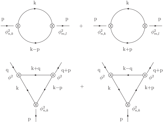
Figure 1: The propagator of the composite operator, $\langle\phi^{2}_{n,k}\,\phi^{2}_{m,l}\rangle$, and the Green function $\langle\phi^{2}\,\phi^{2}\,\phi^{2}_{n,k}\rangle$ in free scalar field theory.

Let us demonstrate that our main formula (2) gives the same result (3). To do this, one has to calculate both the propagator of the composite operator, $\langle\phi^{2}_{m,l}\,\phi^{2}_{n,k}\rangle$, and 3-point Green function $\langle\phi^{2}\,\phi^{2}\,\phi^{2}_{n,k}\rangle$. The corresponding diagrams are presented in Fig. 1. The vertex which corresponds to the composite operator $\phi^{2}_{n,k}$ is equal to $(pn)^{n-k}\,(kn)^{k}$, with $k$ and $(k-p)$ being ingoing and outgoing 4-momentum, respectively. The result of our calculations is the following:

$$\langle\phi^{2}_{m,l}\,\phi^{2}_{n,k}\rangle(p^{2}/\bar{\mu}^{2})\Big{|}_{p^{2}\rightarrow 0}=(-1)^{n-1}\frac{1}{16\pi^{2}}\ln\left(\frac{\bar{\mu}^{2}}{-p^{2}}\right)B(l+1,k+1),$$ (39)

and

$$\mathrm{disc}_{(p+q)^{2}}\,\langle\phi^{2}\,\phi^{2}\,\phi^{2}_{n,k}\rangle(x,q^{2}/p^{2})\Big{|}_{p^{2}\rightarrow 0}$$

$$=i(-1)^{n-1}\,\frac{1}{4\pi}\,\frac{1}{-q^{2}+i0}\,\ln\left(\frac{q^{2}}{p^{2}}\right)\,x\big{[}(1-x)^{k}+x^{k}\big{]}.$$ (40)

The quantity $B(x,y)$ is the beta-function, $B(x,y)=B(y,x)$.

In order to get a finite result for free scalar propagator (39), we had to make a renormalization. As is well known, any Green function with an insertion of one composite operator is multiplicatively renormalized [13, 14]. The renormalization of Green functions with the insertion of two (or more) composite operators needs additive counterterms [12]. The details can be found in Appendix B.

Form formulae (39), (3) and (2) (taking into account the factor in front of the sum in Eq. (36)), we obtain a set of equations for CF’s:

$$\sum_{l=0}^{m}C_{m,l}\,B(l+1,k+1)=\frac{1}{2}\,\left[B(m+1,k+1)+\frac{1}{m+k+1}\right].$$ (41)

It is easy to check that C-numbers $C_{m,l}$ (3) do obey equations (41) for all $m,\,k\geqslant 0$ (for this purpose, formula (A.1) from Appendix A should be used).

4 Calculations of coefficient functions in
perturbative QCD

In this section we will use our formula (2) for calculations of the OPE CF’s in perturbative QCD. For the composite operator, we will often use a brief notation $O^{m,l}$ instead of $O^{m,l}_{\mu_{1}\ldots\mu_{m}}(0)$. Contrary to the matrix element of $O^{m,l}$ between one-particle (quark) states, $\langle p\,|\,O^{m,l}\,|\,p\rangle$, which defines nonsinglet quark distributions in DIS, a propagator $\langle O^{m,l}O^{n,k}\rangle$ is divergent already in zero order in the strong coupling $\alpha_{s}$. The matrix element $\langle J\,J\,O^{n,k}\rangle(Q^{2},x,p^{2})$ is also divergent, whereas its discontinuity in variable $(p+q)^{2}$ is not. The 2-point Green function $\langle O^{m,l}(x)O^{n,k}(y)\rangle$, is renormalized by a subtraction of a contact term of the form $(Z^{-1})^{l}_{l^{\prime}}\,(Z^{-1})^{k}_{k^{\prime}}\,f_{B}^{l^{\prime}k^{\prime}}\delta(x-y)$, where $Z$ is the renormalization matrix of the composite operators. The details can be found in Appendix B.

We work in the dimensional regularization and use the $\overline{\mathrm{MS}}$-scheme to renormalize ultra-violet divergences. Although all calculations will be done in the Feynman gauge, our results are gauge invariant since we sum all diagrams in each order of perturbation theory. Remember that in order to find the OPE CF’s, we have to retain only leading terms in the limit $p^{2}\rightarrow 0$. This simplifies our calculations significantly. We will restrict ourselves by considering leading terms in $\ln(Q^{2}/\mu^{2})$, although our formula (2) enables one to calculate sub-leading terms as well. In other words, along with the limit $p^{2}\rightarrow 0$, we are interested in large values of $Q^{2}$.

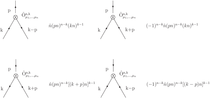
Figure 2: Feynman rules for the composite operators $O^{n,k}_{\mu_{1}\ldots\mu_{n}}$ in the leading (zero) order in strong coupling $\alpha_{s}$.

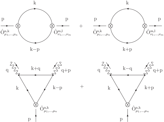
Figure 4: The diagrams for the propagator of the composite operator $\langle O^{n,k}O^{m,l}\rangle^{(0)}$ and for the matrix element $\langle JJ\,O^{n,k}\rangle^{(0)}$.

Let us start from the leading (zero) order in $\alpha_{s}$. The corresponding Feynman diagrams are shown in Fig. 4. All diagrams have logarithmic singularity at $p^{2}\rightarrow 0$. They can be easily calculated with the use of Feynman rules for the composite operators presented in Fig. 2. Note that a vertex which corresponds to the composite operator is not symmetric with respect to ingoing and outgoing momenta. For a particular case with $k=n$, $p=0$, we reproduce the well-known expressions (see the first paper in Refs. [15]).

The result of our calculations in the leading order in the coupling constant is the following:

$$\langle O^{m,l}O^{n,k}\rangle^{(0)}(p^{2}/\bar{\mu}^{2})=(-1)^{n-1}\frac{1}{2\pi^{2}}\ln\left(\frac{\bar{\mu}^{2}}{-p^{2}}\right)B(l+1,k+1),$$ (42)

and

$$\mathrm{disc}_{(p+q)^{2}}\,\langle J\,J\,O^{n,k}\rangle^{(0)}(x,Q^{2}/p^{2})$$

$$=i(-1)^{n-1}\,\frac{e^{2}_{q}}{2\pi}\,\ln\left(\frac{Q^{2}}{-p^{2}}\right)\,\big{[}x(1-x)^{k}-(1-x)x^{k}\big{]},$$ (43)

where $e^{2}_{q}$ is an electric charge of a quark inside a loop. The terms in square brackets in Eq. (4) correspond to two bottom diagrams in Fig. 4 with opposite directions of the quark momentum inside the loop. As for two top diagrams in Fig. 4, they are identical. So, only one of these diagrams was taken into account in Eq. (42). The formula (42) gives a finite (singular at $p^{2}\rightarrow 0$) part of the composite operator propagator (see our comments after Eq. (3)).

Equating factors in front of $\ln(-p^{2})$ in both sides of Eq. (42), (4), and putting $k=1,2,\ldots m$, we obtain the following set of $m$ equations:

$$\sum\limits_{l=1}^{m}\tilde{C}_{m,l}^{(0)}\,B(l+1,k+1)=\frac{1}{2\pi}\int\limits_{0}^{1}\!dx\,x^{m}\,(1-x)[(1-x)^{k-1}-x^{k-1}]$$

$$=\frac{1}{2}\left[B(m+1,k+1)-\frac{1}{(m+k)(m+k+1)}\right]\,,\quad k=1,2,\ldots m.$$ (44)

Using formulae (A.2)-(A.5) from Appendix A, we find the solution of these equations in the form

$$\tilde{C}_{m,m}^{(0)} = \frac{e_{q}^{2}}{2}\,[1+(-1)^{m}],$$ (45)

$$\tilde{C}_{m,l}^{(0)} = \frac{e_{q}^{2}}{2}\,(-1)^{l}{m-1\choose{l-1}},\qquad l=1,2,\ldots,m-1,$$ (46)

where ${n\choose{k}}$ denotes a binomial coefficient. Let us stress, the quantities $\tilde{C}_{m,l}$ (46) satisfy equation (4) for all integer $k\geqslant 1$, although for our purpose it was enough to take $m$ values of $k$.

One can check that

$$\sum_{l=1}^{m}\,\tilde{C}_{m,l}^{(0)}\,\frac{1}{(l+1)(l+2)}=0$$ (47)

(see Eq. (A.5)). Note that the RHS of Eq. (2) is identically equal to zero for $k=1$. Indeed, $\langle J\,J\,O^{1,1}\rangle(x,Q^{2}/p^{2})=0$ due to the Furry theorem. On the other hand, Eq. (42) means that $\langle O^{1,1}O^{m,l}\rangle^{(0)}\sim[(l+1)(l+2)]^{-1}$. We conclude, it is the relation (47) due to which Eq. (2) is satisfied in the leading order in $\alpha_{s}$. As we will see below, a similar relation is valid for $\tilde{C}_{m,l}^{(1)}$ as well.

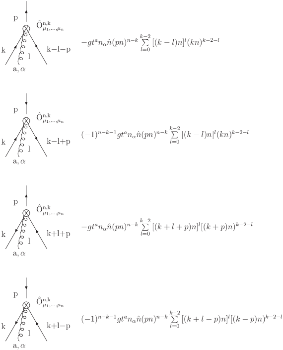
Figure 3: Feynman rules for the composite operators $O^{n,k}_{\mu_{1}\ldots\mu_{n}}$ in the first order in strong coupling $\alpha_{s}$.

Now let us consider the next order in $\alpha_{s}$. The diagrams describing propagator of the composite operator in this order are presented in Figs. 5a, 5b and 6. Using Feynman rules for the composite operators shown in Fig. 3, we obtain the following contribution of the diagrams in Fig. 5a:

$$\langle O^{n,k}O^{m,l}\rangle^{(1)}_{a}(p^{2}/\mu^{2})=(-1)^{n-1}\frac{\alpha_{s}}{8\pi^{3}}\,C_{F}\ln\left(\frac{\bar{\mu}^{2}}{-p^{2}}\right)\,\ln\left(\frac{\mu^{2}}{-p^{2}}\right)$$

$$\times\Bigg{\{}\,\frac{2}{k(k+1)}\,\Bigg{[}B(l+1,k+1)+\sum_{j=1}^{k-1}B(l+1,j+1)\Bigg{]}$$

$$-B(l+1,k+1)+(k\rightleftarrows l)\Bigg{\}},$$ (48)

where $C_{F}=(N_{c}^{2}-1)/2N_{c}$, with $N_{c}$ being a number of colors. For the diagrams in Fig. 5b, we get the expression:

$$\langle O^{n,k}O^{m,l}\rangle^{(1)}_{b}(p^{2}/\mu^{2})=(-1)^{n-1}\frac{\alpha_{s}}{4\pi^{3}}\,C_{F}\ln\left(\frac{\bar{\mu}^{2}}{-p^{2}}\right)\,\ln\left(\frac{\mu^{2}}{-p^{2}}\right)$$

$$\times\left[\left(-2\sum_{j=2}^{k}\frac{1}{j}\right)B(l+1,k+1)\right.$$

$$+\left.\sum_{j=1}^{k-1}\left(\frac{1}{k-j}-\frac{1}{k}\right)B(l+1,j+1)+(k\rightleftarrows l)\right]$$ (49)

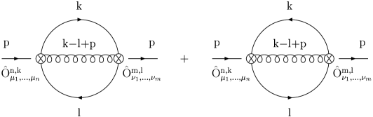
Figure 6: The diagrams which give zero contribution to the propagator $\langle O^{n,k}O^{m,l}\rangle^{(1)}$.

Both diagrams in Fig. 6 are equal to zero since they are proportional to $n_{\mu}^{2}$. Thus, the sum of diagrams which make a contribution to the propagator of the composite operator is given by

$$\langle O^{n,k}O^{m,l}\rangle^{(1)}(p^{2}/\mu^{2})=(-1)^{n-1}\frac{\alpha_{s}}{8\pi^{3}}\,C_{F}\ln\left(\frac{\bar{\mu}^{2}}{-p^{2}}\right)\,\ln\left(\frac{\mu^{2}}{-p^{2}}\right)$$

$$\times\left[\left(-4\sum_{j=2}^{k}\frac{1}{j}-1+\frac{2}{k(k+1)}\right)\right.B(l+1,k+1)$$

$$+\,2\,\left.\sum_{j=1}^{k-1}\left(\frac{1}{k-j}-\frac{1}{k+1}\right)B(l+1,j+1)+(k\rightleftarrows l)\right].$$ (50)

Note, that $\langle O^{n,k}O^{m,l}\rangle^{(1)}=0$ for $k=1$ or $l=1$. Equation (4) can be presented in the form:

$$\langle O^{n,k}O^{m,l}\rangle^{(1)}(p^{2}/\mu^{2})=\frac{\alpha_{s}}{4\pi}\,C_{F}\ln\left(\frac{\mu^{2}}{-p^{2}}\right)$$

$$\times\left[\langle O^{n,k}O^{m,l}\rangle^{(0)}(p^{2}/\bar{\mu}^{2})\left(-4\sum_{j=2}^{k}\frac{1}{j}-1+\frac{2}{k(k+1)}\right)\right.$$

$$+\left.2\sum_{j=1}^{k-1}\left(\frac{1}{k-j}-\frac{1}{k+1}\right)\,\langle O^{n,j}O^{m,l}\rangle^{(0)}(p^{2}/\bar{\mu}^{2})+(k\rightleftarrows l)\right].$$ (51)

For our further purposes, it is useful to present (4) in a form which has no explicit symmetry in $l$ and $k$:

$$\langle O^{n,k}O^{m,l}\rangle^{(1)}(p^{2}/\mu^{2})=(-1)^{n-1}\frac{\alpha_{s}}{4\pi^{3}}\,C_{F}\ln\left(\frac{\bar{\mu}^{2}}{-p^{2}}\right)\,\ln\left(\frac{\mu^{2}}{-p^{2}}\right)$$

$$\times\left[\left(-4\sum_{j=2}^{k}\frac{1}{j}-1+\frac{2}{k(k+1)}\right)\right.B(l+1,k+1)$$

$$+\,2\left.\sum_{j=1}^{k-1}\left(\frac{1}{k-j}-\frac{1}{k+1}\right)B(l+1,j+1)\right].$$ (52)

In deriving Eq. (4) from Eq. (4), the formulae from the Appendix A were used. Taking into account (46), we find

$$\sum_{l=1}^{m}\,\tilde{C}_{m,l}^{(0)}\,\langle O^{n,k}O^{m,l}\rangle^{(1)}(p^{2}/\mu^{2})=(-1)^{n-1}\,e_{q}^{2}\,\frac{\alpha_{s}}{8\pi^{3}}\,C_{F}\ln\left(\frac{\bar{\mu}^{2}}{-p^{2}}\right)\,\ln\left(\frac{\mu^{2}}{-p^{2}}\right)$$

$$\times\left\{[1+(-1)^{m}]\left[\left(-4\sum_{j=2}^{k}\frac{1}{j}-1+\frac{2}{k(k+1)}\right)B(m+1,k+1)\right.\right.$$

$$+\left.2\,\sum_{j=1}^{k-1}\left(\frac{1}{k-j}-\frac{1}{k+1}\right)B(m+1,j+1)\right]$$

$$+\sum_{l=1}^{m-1}(-1)^{l}{m-1\choose{l-1}}\left[\left(-4\sum_{j=2}^{k}\frac{1}{j}-1+\frac{2}{k(k+1)}\right)B(l+1,k+1)\right.$$

$$+\left.\left.2\,\sum_{j=1}^{k-1}\left(\frac{1}{k-j}-\frac{1}{k+1}\right)B(l+1,j+1)\right]\right\}.$$ (53)

As one can see from (4), $\sum_{l=1}^{m}\,\tilde{C}_{m,l}^{(0)}\,\langle O^{n,k}O^{m,l}\rangle^{(1)}=0$ for $k=1$ and $m=1$.

The expression (4) can be simplified and presented as

$$\sum_{l=1}^{m}\,\tilde{C}_{m,l}^{(0)}\,\langle O^{n,k}O^{m,l}\rangle^{(1)}(p^{2}/\mu^{2})=(-1)^{n-1}\,e_{q}^{2}\,\frac{\alpha_{s}}{8\pi^{3}}\,C_{F}\ln\left(\frac{\bar{\mu}^{2}}{-p^{2}}\right)\,\ln\left(\frac{\mu^{2}}{-p^{2}}\right)$$

$$\times\left\{\left(-4\sum_{j=2}^{k}\frac{1}{j}-1+\frac{2}{k}+\frac{2}{m}\right)\right.\left[B(m+1,k+1)-\frac{1}{(m+k)(m+k+1)}\right]$$

$$+\,2\,\sum_{j=2}^{k-1}\frac{1}{k-j}\left[B(m+1,j+1)-\frac{1}{(m+j)(m+j+1)}\right]$$

$$+\left.\frac{2(m-1)(k-1)}{m(m+1)(k+1)(m+k)}\right\}.$$ (54)

With the use of Eq. (Appendix A) from Appendix A, one can rewrite (4) in the form which has an explicit symmetry in $k,m$:

$$\sum_{l=1}^{m}\,\tilde{C}_{m,l}^{(0)}\,\langle O^{n,k}O^{m,l}\rangle^{(1)}(p^{2}/\mu^{2})=(-1)^{n-1}\,e_{q}^{2}\,\frac{\alpha_{s}}{8\pi^{3}}\,C_{F}\ln\left(\frac{\bar{\mu}^{2}}{-p^{2}}\right)\,\ln\left(\frac{\mu^{2}}{-p^{2}}\right)$$

$$\times\left\{2\left(-\sum_{j=2}^{k}\frac{1}{j}-\sum_{j=2}^{m}\frac{1}{j}+1+\frac{2}{k}+\frac{2}{m}\right)\right.$$

$$\times\left[B(m+1,k+1)-\frac{1}{(m+k)(m+k+1)}\right]$$

$$+\left[\sum_{j=1}^{k-1}\frac{1}{k-j}\,B(m+1,j+1)+\sum_{j=1}^{m-1}\frac{1}{m-j}\,B(k+1,j+1)\right]$$

$$-\left.\frac{2}{(m+k)(m+k+1)}\sum_{j=2}^{m+k-1}\frac{1}{j}\,+\,\frac{2-(m+k)}{k(k+1)m(m+1)}\right\}.$$ (55)

Now let us calculate the Green function which contains one composite operator and two electromagnetic currents. The diagrams in Fig. 7a give

$$\mathrm{disc}_{(p+q)^{2}}\,\langle J\,J\,O^{n,k}\rangle^{(1)}_{a}(x,Q^{2}/p^{2},p^{2}/\mu^{2})$$

$$=i(-1)^{n-1}\,e_{q}^{2}\,\frac{\alpha_{s}}{8\pi^{2}}\,C_{F}\ln\left(\frac{Q^{2}}{-p^{2}}\right)\,\ln\left(\frac{\mu^{2}}{-p^{2}}\right)$$

$$\times\Bigg{\{}\Bigg{[}\frac{2}{k(k+1)}-1\Bigg{]}\,\Big{[}x(1-x)^{k}-(1-x)x^{k}\Big{]}$$

$$+\frac{2}{k(k+1)}\,\sum_{j=2}^{k-1}\,\Big{[}x(1-x)^{j}-(1-x)x^{j}\Big{]}\Bigg{\}}.$$ (56)

The equation (4) can be rewritten as follows:

$$\mathrm{disc}_{(p+q)^{2}}\,\langle J\,J\,O^{n,k}\rangle^{(1)}_{a}(x,Q^{2}/p^{2},p^{2}/\mu^{2})=\frac{\alpha_{s}}{4\pi}\,C_{F}\ln\left(\frac{\mu^{2}}{-p^{2}}\right)$$

$$\times\Bigg{\{}\Bigg{[}\frac{2}{k(k+1)}-1\Bigg{]}\,\mathrm{disc}_{(p+q)^{2}}\,\langle J\,J\,O^{n,k}\rangle^{(0)}(x,Q^{2}/p^{2})$$

$$+\frac{2}{k(k+1)}\,\sum_{j=1}^{k-1}\,\mathrm{disc}_{(p+q)^{2}}\,\langle J\,J\,O^{n,j}\rangle^{(0)}(x,Q^{2}/p^{2})\Bigg{\}},$$ (57)

with zero order expression given by (4).

The contribution from the sum of the diagrams in Fig. 7b is equal to

$$\mathrm{disc}_{(p+q)^{2}}\,\langle J\,J\,O^{n,k}\rangle^{(1)}_{b}(x,Q^{2}/p^{2},p^{2}/\mu^{2})$$

$$=i(-1)^{n-1}\,e_{q}^{2}\,\frac{\alpha_{s}}{4\pi^{2}}\,C_{F}\ln\left(\frac{Q^{2}}{-p^{2}}\right)\,\ln\left(\frac{\mu^{2}}{-p^{2}}\right)$$

$$\times\left\{-2\sum_{j=2}^{k}\frac{1}{j}\,\,\Big{[}x(1-x)^{k}-(1-x)x^{k}\Big{]}\right.$$

$$+\left.\,\sum_{j=2}^{k-1}\left(\frac{1}{k-j}-\frac{1}{k}\right)\,\Big{[}x(1-x)^{j}-(1-x)x^{j}\Big{]}\right\}.$$ (58)

Note again that Eq. (4) can be rewritten in terms of an absorptive part of the 3-point Green function calculated in the leading order in $\alpha_{s}$:

$$\mathrm{disc}_{(p+q)^{2}}\,\langle J\,J\,O^{n,k}\rangle^{(1)}_{b}(x,Q^{2}/p^{2},p^{2}/\mu^{2})=\frac{\alpha_{s}}{2\pi}\,C_{F}\ln\left(\frac{\mu^{2}}{-p^{2}}\right)$$

$$\times\left\{\left(-2\sum_{j=2}^{k}\frac{1}{j}\right)\mathrm{disc}_{(p+q)^{2}}\,\langle J\,J\,O^{n,k}\rangle^{(0)}(x,Q^{2}/p^{2})\right.$$

$$+\left.\sum_{j=1}^{k-1}\left(\frac{1}{k-j}-\frac{1}{k}\right)\mathrm{disc}_{(p+q)^{2}}\,\langle J\,J\,O^{n,j}\rangle^{(0)}(x,Q^{2}/p^{2})\right\}.$$ (59)

The diagram in Fig. 8 is sub-leading at $p^{2}\rightarrow 0$, since it has no singularities at $p_{\mu}=0$. The diagrams in Figs. 9a and 9b describe a renormalization of the electromagnetic current $J^{em}$ which is conserved and, therefore, has no anomalous dimensions. As a result, these diagrams are suppressed by the inverse of $\ln(\mu^{2}/(-p^{2}))$ with respect to (4) and (4). Thus, we have to sum only expressions (4) and (4):

$$\frac{1}{2\pi}\int\limits_{0}^{1}\!dxx^{m-1}\,\mathrm{disc}_{(p+q)^{2}}\,\langle J\,J\,O^{n,k}\rangle^{(1)}(x,Q^{2}/p^{2},p^{2}/\mu^{2})$$

$$=i(-1)^{n-1}\,e_{q}^{2}\,\frac{\alpha_{s}}{8\pi^{3}}\,C_{F}\ln\left(\frac{Q^{2}}{-p^{2}}\right)\,\ln\left(\frac{\mu^{2}}{-p^{2}}\right)$$

$$\times\left\{\left(-4\sum_{j=2}^{k}\frac{1}{j}\,-1+\frac{2}{k}\right)\right.\left[B(m+1,k+1)-\frac{1}{(m+k)(m+k+1)}\right]$$

$$+\,2\,\sum_{j=2}^{k-1}\frac{1}{k-j}\left[B(m+1,j+1)-\frac{1}{(m+j)(m+j+1)}\right]$$

$$-\,\frac{2}{k+1}\left[B(m+1,k+1)-\frac{1}{(m+k)(m+k+1)}\right]$$

$$-\left.\frac{2}{k+1}\sum_{j=2}^{k-1}\left[B(m+1,j+1)-\frac{1}{(m+j)(m+j+1)}\right]\right\}.$$ (60)

Making use of equation (Appendix A), one can easily calculate the sum in the last line of equation (4) and rewrite it in the form:

$$\frac{1}{2\pi}\int\limits_{0}^{1}\!dxx^{m-1}\,\mathrm{disc}_{(p+q)^{2}}\,\langle J\,J\,O^{n,k}\rangle^{(1)}(x,Q^{2}/p^{2},p^{2}/\mu^{2})$$

$$=i(-1)^{n-1}\,e_{q}^{2}\,\frac{\alpha_{s}}{8\pi^{3}}\,C_{F}\ln\left(\frac{Q^{2}}{-p^{2}}\right)\,\ln\left(\frac{\mu^{2}}{-p^{2}}\right)$$

$$\times\left\{\left(-4\sum_{j=2}^{k}\frac{1}{j}-1+\frac{2}{k}+\frac{2}{m}\right)\right.\left[B(m+1,k+1)-\frac{1}{(m+k)(m+k+1)}\right]$$

$$+\,2\,\sum_{j=2}^{k-1}\frac{1}{k-j}\left[B(m+1,j+1)-\frac{1}{(m+j)(m+j+1)}\right]$$

$$+\frac{2(m-1)(k-1)}{m(m+1)(k+1)(m+k)}\Bigg{\}}.$$ (61)

The set of equations for the OPE CF’s $\tilde{C}_{m,l}^{(1)}(Q^{2}/\mu^{2})$ ($l=1,2,\ldots m$) looks like:

$$\sum_{l=1}^{m}\,\tilde{C}_{m,l}^{(1)}(Q^{2}/\mu^{2})\,\langle O^{n,k}O^{m,l}\rangle^{(0)}(p^{2})+\sum_{l=1}^{m}\,\tilde{C}_{m,l}^{(0)}\,\langle O^{n,k}O^{m,l}\rangle^{(1)}(p^{2})$$ (62)

$$=\frac{1}{2\pi i}\int\limits_{0}^{1}\!dxx^{m-1}\,\mathrm{disc}_{(p+q)^{2}}\,\langle J\,J\,O^{n,k}\rangle^{(1)}(x,Q^{2}/p^{2},p^{2}/\mu^{2}).$$

From (62) and (4), (4) one, therefore, can get $m$ equations,

$$\sum_{l=1}^{m}\,\tilde{C}_{m,l}^{(1)}(Q^{2}/\mu^{2})\,B(l+1,k+1)=\,e_{q}^{2}\,\frac{\alpha_{s}}{8\pi}\,C_{F}\ln\left(\frac{Q^{2}}{\mu^{2}}\right)$$

$$\times\left\{\left(-4\sum_{j=2}^{k}\frac{1}{j}-1+\frac{2}{k}+\frac{2}{m}\right)\right.\left[B(m+1,k+1)-\frac{1}{(m+k)(m+k+1)}\right]$$

$$+\,2\,\sum_{j=2}^{k-1}\frac{1}{k-j}\left[B(m+1,j+1)-\frac{1}{(m+j)(m+j+1)}\right]$$

$$+\frac{2(m-1)(k-1)}{m(m+1)(k+1)(m+k)}\Bigg{\}},$$ (63)

for $m$ different values of $k=1,2\ldots m$. In particular, we obtain for $k=1$:

$$\sum_{l=1}^{m}\,\tilde{C}_{m,l}^{(1)}(Q^{2}/\mu^{2})\,\frac{1}{(l+1)(l+2)}=0.$$ (64)

This equation is similar to formula (47) which was obtained in the leading order.

However, in order to find $\tilde{C}_{m,l}^{(1)}$, it is much more convenient to use equivalent form of the expression in the RHS of Eq. (4) For this purpose, one should compare (4) with (4), and then exploit the above demonstrated symmetry in $k$, $l(k,m)$ (4):

$$\sum_{l=1}^{m}\,\tilde{C}_{m,l}^{(1)}(Q^{2}/\mu^{2})\,B(k+1,l+1)=\,e_{q}^{2}\,\frac{\alpha_{s}}{8\pi}\,C_{F}\ln\left(\frac{Q^{2}}{\mu^{2}}\right)$$

$$\times\left\{[1+(-1)^{m}]\left[\left(-4\sum_{j=2}^{m}\frac{1}{j}-1+\frac{2}{m(m+1)}\right)B(k+1,m+1)\right.\right.$$

$$+\left.2\,\sum_{j=1}^{m-1}\left(\frac{1}{m-j}-\frac{1}{m+1}\right)B(k+1,j+1)\right]$$

$$+\sum_{l=1}^{m-1}(-1)^{l}{m-1\choose{l-1}}\left[\left(-4\sum_{j=2}^{l}\frac{1}{j}-1+\frac{2}{l(l+1)}\right)B(k+1,l+1)\right.$$

$$+\left.\left.2\,\sum_{j=1}^{l-1}\left(\frac{1}{l-j}-\frac{1}{l+1}\right)B(k+1,j+1)\right]\right\}.$$ (65)

Thus, we get $m$ equations (corresponding to $k=1,2\ldots m$) for $m$ coefficient functions. The solution of these equations (4) is rather easy to find, the result is

$$\tilde{C}_{m,m}^{(1)}(Q^{2}/\mu^{2})=e_{q}^{2}\,\frac{\alpha_{s}}{8\pi}\,C_{F}\ln\left(\frac{Q^{2}}{\mu^{2}}\right)\,$$

$$\times[1+(-1)^{m}]\left[-4\sum_{j=2}^{m}\frac{1}{j}-1+\frac{2}{m(m+1)}\right],$$ (66)

and

$$\tilde{C}_{m,l}^{(1)}(Q^{2}/\mu^{2})=e_{q}^{2}\,\frac{\alpha_{s}}{4\pi}\,C_{F}\ln\left(\frac{Q^{2}}{\mu^{2}}\right)$$

$$\times\left\{\frac{1}{2}(-1)^{l}{m-1\choose{l-1}}\left[-4\sum_{j=2}^{l}\frac{1}{j}-1+\frac{2}{l(l+1)}\right]\right.$$

$$+\left(\frac{1}{m-l}-\frac{1}{m+1}\right)$$

$$+\left.\sum_{k=l+1}^{m}(-1)^{k}{m-1\choose{k-1}}\left(\frac{1}{k-l}-\frac{1}{k+1}\right)\right\},$$ (67)

for $l=1,2,\ldots,m-1$. We used formulae for summation in $l$ ((A.5), (Appendix A)) and $j$ ((A.11)) from Appendix A. In particular, we get from (4) ($m\geqslant 2$):

$$\tilde{C}_{m,1}^{(1)}=e_{q}^{2}\,\frac{\alpha_{s}}{4\pi}\,C_{F}\ln\left(\frac{Q^{2}}{\mu^{2}}\right)\Bigg{[}\sum_{j=1}^{m}\frac{1}{j}-\frac{1}{2}+\frac{1}{m-1}-\frac{2}{m+1}\Bigg{]}.$$ (68)

As one can see from (4), “major” coefficient function $\tilde{C}_{m,m}^{(1)}$ is defined by well-known anomalous dimension of $O^{m,m}$ [4],

$$\gamma^{{}_{NS}}_{m}=\frac{\alpha_{s}}{2\pi}\,C_{F}\,\left[4\sum_{j=2}^{m}\frac{1}{j}+1-\frac{2}{m(m+1)}\right],$$ (69)

in spite of the fact that $O^{m,m}$ mixes with all operators $O^{m,l}$ ($l=1,2.\ldots m$) under the renormalization. We have reproduced the standard expression for the coefficient function $\tilde{C}_{m,m}(Q^{2}/\mu^{2})$, and, simultaneously, have calculated “gradient” OPE coefficient functions $\tilde{C}_{m,l}(Q^{2}/\mu^{2})$ ($l=1,2.\ldots m-1$) in zero and first order in $\alpha_{s}$ (see Eqs. (46) and (4)).

Let us emphasize that our operator definition of the coefficient functions $C^{m,l}(Q^{2}/\mu^{2})$ (31) results in a homogeneous renormalization group equation for $C^{m,l}(Q^{2}/\mu^{2})$ with respect to $\mu$, in spite of the fact that composite operator Green functions $\langle O^{n,k}O^{m,l}\rangle$ need an additional renormalization. The details are discussed in Appendix B.

5 Finite renormalization of composite
operators and rescaling of coefficient
functions

With accounting for equations (45), (46) and (4), (4), the expressions for the OPE CF’s can be rewritten in the following form:

$$\tilde{C}_{m,m}(Q^{2}/\mu^{2}) = \tilde{C}_{m,m}^{(0)}\,\Bigg{\{}1+\frac{\alpha_{s}}{4\pi}\,C_{F}\ln\left(\frac{Q^{2}}{\mu^{2}}\right)$$ (70)

$$\times \left[-4\sum_{j=2}^{m}\frac{1}{j}-1+\frac{2}{m(m+1)}\right]\Bigg{\}},$$

$$\tilde{C}_{m,l}(Q^{2}/\mu^{2}) = \tilde{C}_{m,l}^{(0)}\,\Bigg{\{}1+\frac{\alpha_{s}}{4\pi}\,C_{F}\ln\left(\frac{Q^{2}}{\mu^{2}}\right)\left[-4\sum_{j=2}^{l}\frac{1}{j}-1+\frac{2}{l(l+1)}\right]\Bigg{\}}$$ (71)

$$+ \frac{\alpha_{s}}{2\pi}\,C_{F}\ln\left(\frac{Q^{2}}{\mu^{2}}\right)\,\sum_{k=l+1}^{m}\tilde{C}_{m,k}^{(0)}\,\left(\frac{1}{k-l}-\frac{1}{k+1}\right),$$

for $l=1,2,\ldots,m-1$.

Let us consider a sum of products of renormalized composite operators and corresponding CF’s which enter the OPE of two electromagnetic currents (4). According to (12), the renormalized composite operator $O^{m,l}_{R}(\mu_{1}^{2})$ is changed under rescaling $\mu_{1}\rightarrow\mu_{2}$ as follows

$$O^{m,l}_{R}(\mu_{1}^{2})=\sum_{l^{\prime}=1}^{l}\hat{Z}^{l}_{l^{\prime}}(\mu_{2}^{2}/\mu_{1}^{2})\,O^{m,l^{\prime}}_{R}(\mu_{2}^{2}),$$ (72)

where $\mu_{i}$ denotes a renormalization scale of the composite operators in the $\overline{\mathrm{MS}}$-scheme, and $\mathbf{\hat{Z}}$ is a matrix of a finite renormalization. Let us emphasize that due to Eq. (B.9)

$${\langle O^{m,l}O^{n,k}\rangle}_{R}(\mu_{1}^{2})=\sum_{l^{\prime}=1}^{l}\hat{Z}^{l}_{l^{\prime}}(\mu_{2}^{2}/\mu_{1}^{2})\sum_{k^{\prime}=1}^{k}\hat{Z}^{k}_{k^{\prime}}(\mu_{2}^{2}/\mu_{1}^{2})\,{\langle O^{m,l^{\prime}}O^{n,k^{\prime}}\rangle}_{R}(\mu_{2}^{2}),$$ (73)

since additive coefficients in Eq. (B.9) do not depent on the renormalization scale $\mu$.

In the first order of strong interaction, the matrix looks like

$$\hat{Z}_{ll^{\prime}}=\left\{\begin{array}[]{cl}\displaystyle 1+C_{F}\,\frac{\alpha_{s}}{4\pi}\,\ln\left(\frac{\mu_{2}^{2}}{\mu_{1}^{2}}\right)\Big{[}-4\sum\limits_{j=2}^{l}\frac{1}{j}-1+\frac{2}{l(l+1)}\Big{]},&l^{\prime}=l,\\ \displaystyle C_{F}\,\frac{\alpha_{s}}{2\pi}\,\ln\left(\frac{\mu_{2}^{2}}{\mu_{1}^{2}}\right)\Big{[}\frac{1}{l-l^{\prime}}-\frac{1}{l+1}\Big{]},&l^{\prime}<l\\ 0,&l^{\prime}>l\\ \end{array}\right.$$ (74)

In a general case we find:

$$\sum_{l=1}^{m}\tilde{C}_{m,l}\,O^{m,l}_{R}(\mu_{1}^{2}) = \sum_{l=1}^{m}\tilde{C}_{m,l}\sum_{l^{\prime}=1}^{l}\hat{Z}^{l}_{l^{\prime}}(\mu_{2}^{2}/\mu_{1}^{2})\,O^{m,l^{\prime}}_{R}(\mu_{2}^{2})$$ (75)

$$= \sum_{l=1}^{m}\tilde{C}_{m,l}(\mu_{2}^{2}/\mu_{1}^{2})\,O^{m,l}_{R}(\mu_{2}^{2}),$$

where

$$\tilde{C}_{m,l}(\mu_{2}^{2}/\mu_{1}^{2})=\sum_{k=1}^{m}\tilde{C}_{m,k}\,\hat{Z}^{k}_{l}(\mu_{2}^{2}/\mu_{1}^{2}).$$ (76)

Thus, we obtain from (76)

$$\tilde{C}_{m,m}(\mu_{2}^{2}/\mu_{1}^{2})=\tilde{C}_{m,m}\,\hat{Z}^{m}_{m}(\mu_{2}^{2}/\mu_{1}^{2}),$$ (77)

$$\tilde{C}_{m,l}(\mu_{2}^{2}/\mu_{1}^{2})=\tilde{C}_{m,l}\,\hat{Z}^{l}_{l}(\mu_{2}^{2}/\mu_{1}^{2})+\sum_{k=l+1}^{m}\tilde{C}_{m,k}\,\hat{Z}^{k}_{l}(\mu_{2}^{2}/\mu_{1}^{2}),$$ (78)

for $l=1,2,\ldots,m-1$. It was taken into account that $\hat{Z}_{kl}=0$ for $k<l$. Thus, if one changes the renormalization scale $\mu$, the “major” coefficient function $\tilde{C}_{m,m}$ is simply multiplied by the factor $\hat{Z}_{mm}$, while the other CF’s mix with each other. It is a consequence of the fact that the matrix $\hat{Z}_{kl}$ has a triangle form with zero elements above its diagonal.

The coefficient functions $\tilde{C}_{m,l}(\mu_{2}^{2}/\mu_{1}^{2})$ are normalized so that $\tilde{C}_{m,l}(1)=\tilde{C}_{m,l}$, where numbers $\tilde{C}_{m,l}$ are “bare” coefficient functions which were obtained for the case with no strong interactions (see Eqs. (45), (46)). We conclude from explicit expression of $\mathbf{\hat{Z}}$ in the first order in $\alpha_{s}$ (74) that our perturbative result, equations (70) and (71), is a particular case of general formulae (77) and (78).

6 Conclusions

As was shown above, the OPE coefficient functions can be expressed in terms of the Green functions of the corresponding composite operators without explicit use of the elementary (quark and gluon) field operators. We would like to specially stress that our general expression (31) for the OPE coefficient functions holds in any renormalization scheme in contrast with previous prescriptions (see, for instance, [10]). We believe that such a representation is useful in proving general properties of the coefficient functions and for non-perturbative calculations (e.g. in lattice QCD).

We would like to stress that if one assumes the light-cone expansion in the framework of axiomatic approach (see, for instance, Ref. [18]), then our formulae do not lean on perturbative expansions at all and deal with v.e.v. of T-products of local Heisenberg operators.

In this paper we limited ourselves by the QCD nonsinglet operator only. The singlet case needs a special treatment and will be considered in a forthcoming paper.

Appendix A

In this Appendix we have collected formulae which are needed for calculating sums in $l$ and $j$ presented in the text and getting compact expressions. Let us first consider summation in index $l$. For $m\geqslant 0$, we have the relation

$$\sum_{l=0}^{m}(-1)^{l}{m\choose{l}}{l+k+1\choose{l+1}}^{-1}\frac{1}{l+1}=\frac{1}{m+k+1}\,.$$ (A.1)

The quantity ${n\choose{k}}$ is a binomial coefficient. In the following equations, $m\geqslant 1$ is assumed:

$$\sum_{l=1}^{m-1}(-1)^{l}{m-1\choose{l-1}}=-\left[(-1)^{m}+\frac{1}{\Gamma(2-m)}\right],$$ (A.2)

$$\sum_{l=1}^{m-1}(-1)^{l}{m-1\choose{l-1}}\!\frac{1}{l}=-\frac{1}{m}[1+(-1)^{m}],$$ (A.3)

$$\sum_{l=1}^{m-1}(-1)^{l}{m-1\choose{l-1}}\!\frac{1}{l+1}=-\frac{1}{m}+\frac{1}{m+1}[1-(-1)^{m}],$$ (A.4)

$$\sum_{l=1}^{m-1}(-1)^{l}{m-1\choose{l-1}}\!\frac{1}{(l+1)(l+2)}=-\frac{1}{(m+1)(m+2)}[1+(-1)^{m}],$$ (A.5)

$$-2\,\sum_{l=1}^{m-1}\left(\frac{1}{m-l}-\frac{1}{m+1}\right)\frac{1}{(l+1)(l+2)}$$

$$=\frac{1}{(m+1)(m+2)}\left[-4\sum_{j=2}^{m}\frac{1}{j}-1+\frac{2}{m(m+1)}\right],$$ (A.6)

$$\sum_{l=1}^{m-1}(-1)^{l}{m-1\choose{l-1}}{l+k+1\choose{l+1}}^{-1}$$

$$=(-1)^{m+1}{m+k+1\choose{m+1}}^{-1}\!\frac{1}{m+1}-\frac{1}{(m+k)(m+k+1)}\,,$$ (A.7)

$$\sum_{l=1}^{m-1}(-1)^{l}{m-1\choose{l-1}}{l+k+1\choose{l+1}}^{-1}\frac{1}{l}$$

$$=(-1)^{m+1}{m+k+1\choose{m+1}}^{-1}\frac{1}{m}+\frac{k}{(k+1)(m+k+1)}-\frac{1}{m+k}\,,$$ (A.8)

$$\sum_{l=1}^{m-1}(-1)^{l}{m-1\choose{l-1}}{l+k+1\choose{l+1}}^{-1}\!\frac{1}{l(l+1)}$$

$$=(-1)^{m+1}{m+k+1\choose{m+1}}^{-1}\!\frac{1}{m(m+1)}-\frac{1}{(k+1)(m+k+1)}\,.$$ (A.9)

Now let us consider summation in index $j$ ($k,l\geqslant 1$ is assumed everywhere):

$$\sum_{j=1}^{k}{m+k-j-1\choose{m-1}}\frac{1}{j}={m+k-1\choose{k}}\left[\sum_{j=1}^{m+k-1}\frac{1}{j}-\sum_{j=1}^{m-1}\frac{1}{j}\right],$$ (A.10)

$$\sum_{j=1}^{m-1}\frac{1}{j}-\sum_{j=1}^{l-1}\frac{1}{j}={m-1\choose{l-1}}^{-1}\sum_{j=1}^{m-l}{m-j-1\choose{l-1}}\frac{1}{j}\,.$$ (A.11)

Note that the last equation is a particular case of Eq. (A.10) for $1\leq l\leq m$. Let us present other useful formulae:

$$\sum_{j=1}^{l-1}{k+j+1\choose{j}}^{-1}=-\frac{k+l+1}{k}{k+l+1\choose{l}}^{-1}+\frac{1}{k}\,,$$ (A.12)

$$\sum_{j=0}^{l-1}{k+j+1\choose{j}}^{-1}\!\frac{1}{l-j} = {k+l+1\choose{l}}^{-1}$$ (A.13)

$$\times \left[\sum_{j=1}^{l}\frac{1}{j}+\sum_{j=1}^{l}{k+j\choose{j}}\,\frac{1}{j}\right],$$

$$\sum_{j=1}^{l-1}\frac{1}{j}\left[{k+j\choose{j}}-1\right]=\sum_{j=1}^{k-1}\frac{1}{j}\left[{l+j\choose{j}}-1\right],$$ (A.14)

$$\frac{1}{k+1}\left[\sum_{j=0}^{l-1}{k+j+1\choose{j}}^{-1}\!\frac{1}{l-j}-2\,{k+l+1\choose{l}}^{-1}\sum_{j=2}^{l}\frac{1}{j}\right]$$

$$=\!\frac{1}{l+1}\left[\sum_{j=0}^{k-1}{l+j+1\choose{j}}^{-1}\!\frac{1}{k-j}-2\,{l+k+1\choose{k}}^{-1}\sum_{j=2}^{k}\frac{1}{j}\right].$$ (A.15)

The last relation is a consequence of Eqs. (A.13) and (A.14). It demonstrates that the sum in (Appendix A) is symmetric under replacement $l\rightleftarrows k$.

The last useful formula contains sums in $l$ and $j$:

$$\sum_{l=1}^{m-1}(-1)^{l}{m-1\choose{l-1}}{l+k+1\choose{l+1}}^{-1}\!\frac{1}{l+1}\,\sum_{j=1}^{k}{l+j\choose{j}}\frac{1}{j}$$

$$=-\,{m+k+1\choose{m+1}}^{-1}\!\frac{1}{m+1}\left[\sum_{j=0}^{k-1}{m+j-1\choose{j}}\frac{k-j+1}{(k-j)(m+j)}\right.$$

$$+\,(-1)^{m}\left.\sum_{j=1}^{k}{m+j\choose{j}}\frac{1}{j}\right].$$ (A.16)

Appendix B

The goal of this Appendix is to derive a renormalization group equation (see, for instance, [16]) for the CF’s stating from our formula (31). Let us rewrite it in the form:

$$\sum_{l=1}^{m}\tilde{C}_{m,l}\,\langle OO\rangle^{kl}_{R}=\frac{1}{2\pi i}\int\limits_{0}^{1}\!dxx^{m-1}\,\mbox{\rm disc}_{(p+q)^{2}}\,\langle JJO\rangle^{k}_{R}$$ (B.1)

(see our brief notations in the end of Section 2). The renormalized quantity in the RHS of Eq. (B.1) is given by

$$\sum_{n}\langle J|n\rangle\,\langle n|JO^{n,k}\rangle_{R},$$ (B.2)

where $\sum_{n}$ means a sum in a complete set of elementary (quark and gluon) states $|n\rangle$. Let us underline that each state $|n\rangle$ should include at least one quark-antiquark pair (in non-singlet state). It is well-known that a matrix element with an insertion of one composite operator is multiplicatively renormalized (see, for instance, [14]). Therefore, one has the following relation:

$$\langle J|n\rangle_{R}=Z_{J}\langle J|n\rangle_{U}.$$ (B.3)

Since electromagnetic current is conserved, its renormalization constant, $Z_{J}$, does not depend on the renormalization scale, $(d/d\mu)Z_{J}=0$. ,

Now we will show that the matrix element $\langle n|JO^{n,k}\rangle_{R}$ in (B.2) is also multiplicatively renormalized. Consider arbitrary diagram $G$ which contributes to a matrix element with an insertion of two composite operators, $J$ and $O^{k}$. We assume that divergences of all sub-diagrams of $G$ are already removed. Let $G$ to have $(p+2)$ external lines ($p\geqslant 0$), and $q$ internal vertexes. The index of this diagram, $\omega(G)$, is defined by [14]

$$\omega(G)=\sum_{i}^{q}\omega_{i}^{max}+4-\frac{1}{2}\sum_{l}^{p+2}(r_{l}+2)+(\omega_{J}-4)+(\omega_{O^{n,k}}-4).$$ (B.4)

Here $\omega_{i}^{max}$ is a maximal index of internal vertex of a type $i$, and $r_{l}$ is a power of a polynomial corresponding to an external field of a type $l$ ($r_{q}=1$ for a quark line). The quantities $\omega_{J}$ is the dimension of the electromagnetic current, while $\omega_{O^{n,k}}$ is the dimensions of our composite operators. Note that $\omega_{i}^{max}=0$ for all QCD vertexes, and $\omega_{J}=3$.

As for $\omega_{O^{n,k}}$, it is formally equal to $(k+2)$ (only derivatives with respect to quark line momenta have to be taken into account, not total derivatives). In particular, $\omega_{O^{n,1}}=3$. Let us show, however, that effectively $\omega_{O^{n,k}}$ does not depend on $k$, and $\omega_{O^{n,k}}=\omega_{O^{n,1}}$. Let $\{r_{i}\}$ ($i=1,\ldots p+4$) to be a set of external momenta ($p,q$ including), while $\{k_{i}\}$ ($i=1,\ldots m$) to be a set of loop momenta of $G$ (with $m$ being a number of loops). After using the Feynman parametrization and linear transformations from $\{k_{i}\}$ to $\{l_{i}\}$, an analytical expression for the diagram can be written in the form:

$$I(G) = \prod_{j}\int\!dx_{j}\,\delta(1-\sum_{s}x_{s})\sum_{r=0}^{k-1}\,a_{r}(x_{i})$$ (B.5)

$$\times \prod_{i=1}^{m}\int\!\frac{d^{D}l_{i}}{(2\pi)^{D}}\,(l_{m}n)^{r}\,\frac{P(x_{i},l_{i},r_{i})}{D(x_{i},l_{i}^{2},r_{i}r_{j})}\ ,$$

where $x_{i}$ are the Feynman parameters. The change of variables $\{k_{i}\}\rightarrow\{l_{i}\}$ is done so that the denominator in Eq. (B.5) depends on $l_{i}$ only via $l_{i}^{2}$. Notice, the momentum $l_{m}$ is a linear combination of $r_{i}$, and $k_{m}$, ingoing quark momentum for the vertex $O^{n,k}$. The numerator in Eq. (B.5) is a sum of polynomials of $(l_{i}l_{j})$, $(l_{i}r_{j})$ and $(r_{i}r_{j})$. Each polynomial includes at least one scalar product of the vector $n$, namely, $(l_{i}n)$ or $(r_{i}n)$.

After integrating in $d^{D}l_{1},\dots d^{D}l_{m-1}$, we get

$$I(G) = \prod_{j}\int\!dx_{j}\,\delta(1-\sum_{s}x_{s})\sum_{r=0}^{k-1}\,b_{r}(x_{i})$$ (B.6)

$$\times \int\!\frac{d^{D}l}{(2\pi)^{D}}\,(ln)^{r}\,\frac{\bar{P}(x_{i},l,r_{i})}{\tilde{D}(x_{i},l^{2},r_{i}r_{j})}$$

(we denoted $l_{m}=l$). Note that $\mathrm{dim}\bar{D}-\mathrm{dim}\bar{P}=5$. Let us analyze possible terms in $\bar{P}$ which is a polynomial of $l^{2}$, $(lr_{i})$, $(r_{i}r_{j})$, and depends linearly on $(ln)$ or $(r_{i}n)$. The term $(ln)(l^{2})^{(\mathrm{dim}\bar{P}-1)/2}$ results in zero (for even $r$) or an expression proportional to $n^{2}_{\mu}=0$ (for odd $r$) in the dimensional regularization. All other terms proportional to $(ln)$ drop for the same reason (if $r\geqslant 1$) or give finite integrals which converge in the ultra-violet region. One can verify that terms proportional to $(r_{i}n)$ give non-zero convergent integrals only for $r=0$.

Thus, we have to put $\omega_{O^{n,k}}=\omega_{O^{n,1}}=3$ in (B.4). In its turn, it means that $\omega(G)\leqslant-1$, with $\omega(G)=-1$ for $p=1$. In other words, there is no need to introduce a new counterterm $:J(x)O(y):\delta(x-y)$, and, consequently,

$$\langle n|JO^{n,k}\rangle_{R}=Z_{J}^{-1}\sum_{k^{\prime}=1}^{k}(Z^{-1})^{k}_{k^{\prime}}\,\langle n|JO^{n,k^{\prime}}\rangle_{U}.$$ (B.7)

It follows from (B.3), (B.7) that

$$\mathrm{disc}_{(p+q)^{2}}\,\langle JJO\rangle^{k}_{R}=Z_{J}^{-2}\sum_{k^{\prime}=1}^{k}(Z^{-1})^{k}_{k^{\prime}}\,\mathrm{disc}_{(p+q)^{2}}\,\langle JJO\rangle^{k^{\prime}}_{U}.$$ (B.8)

This result is in agreement with perturbative QCD calculations from Section 4.

Now let us turn to the propagators of the composite operators. The renormalization properties of Green functions with insertions of more than one composite operator were studied in details in Ref. [17]. In particular,

$$\langle OO\rangle^{kl}_{R}=\sum_{l^{\prime}=1}^{l}(Z^{-1})^{l}_{l^{\prime}}\sum_{k^{\prime}=1}^{k}(Z^{-1})^{k}_{k^{\prime}}\Big{[}\langle OO\rangle^{k^{\prime}l^{\prime}}_{U}+f_{B}^{k^{\prime}l^{\prime}}\Big{]}.$$ (B.9)

The divergent coefficients $f_{B}^{kl}$ are, in general, non-zero even in the free theory, as it is the case for our quark operators $Q^{n,k}$.

The renormalization matrix of the composite operator $\mathbf{Z}$ depends on a renormalization scale $\mu$, while the coefficients $f_{B}^{kl}$ do not. The renormalized Green function $\langle OO\rangle^{kl}_{R}$ is also $\mu$-dependent, but it does not depend on the regularization scale $\bar{\mu}$. All physical (measurable) quantities should be, of course, $\bar{\mu}$ and $\mu$-independent.

As one can see, Eq. (B.9) which relates renormalized and unrenormalized propagators has an additive term. Nevertheless, renormalization group equations for the propagators and for CF’s have no additive terms. Indeed, acting on both sides of Eq. (B.1) by the operator $\mu d/d\mu=\mu\partial/\partial\mu+\beta(g_{s})\partial/\partial g_{s}$, and taking into account Eqs. (B.8), (B.9), we obtain:

$$\sum_{l=1}^{m}\Big{[}\mu\frac{d}{d\mu}\,\tilde{C}_{m,l}\,\langle OO\rangle^{kl}_{R}-\tilde{C}_{m,l}\sum_{l^{\prime}=1}^{l}\gamma^{l}_{l^{\prime}}\,\langle OO\rangle^{kl^{\prime}}_{R}\Big{]}=0,$$ (B.10)

where

$$\boldsymbol{\gamma}=\mathbf{Z}^{-1}\,\Big{(}\mu^{\prime}\frac{d}{d\mu^{\prime}}\Big{)}\mathbf{Z}$$ (B.11)

is the matrix of anomalous dimensions of the composite operators. Equation (B.10) can be represented in the form:

$$\sum_{l=l}^{m}\langle OO\rangle^{kl}_{R}\,\Big{[}\mu^{\prime}\frac{d}{d\mu^{\prime}}\,\tilde{C}_{m,l}-\sum_{l^{\prime}=l}^{m}\gamma_{l}^{l^{\prime}}\,\tilde{C}_{m,l^{\prime}}\Big{]}=0.$$ (B.12)

Since (B.12) is valid for arbitrary integer $k\geqslant 1$, we derive a set of renormalization group equations for the coefficient functions $\tilde{C}_{m,l}$ ($l=1,2,\ldots m$):

$$\mu\frac{d}{d\mu}\,\tilde{C}_{m,l}-\sum_{l^{\prime}=l}^{m}\gamma_{l}^{l^{\prime}}\,\tilde{C}_{m,l^{\prime}}=0.$$ (B.13)

In particular, the coefficient function $\tilde{C}_{m,m}$, which is relevant for DIS, obeys the following closed equation:

$$\Big{(}\mu\frac{d}{d\mu}-\gamma_{m}^{m}\Big{)}\tilde{C}_{m,m}=0.$$ (B.14)

Remember that $\boldsymbol{\gamma}$ is the matrix of the anomalous dimensions of non-singlet composite operators which enter light-cone OPE (8):

$$\mu\frac{d}{d\mu}\,O^{m,l}+\sum_{l^{\prime}=1}^{l}\gamma^{l}_{l^{\prime}}\,O^{m,l^{\prime}}=0.$$ (B.15)

This renormalization group equation demonstrates again that composite operators mix under the renormalization. After a diagonalization of the renormalization matrix $\mathbf{Z}$ (13), one obtains new operators $\tilde{O}^{m,l}=\sum_{l^{\prime}=1}^{l}A_{l^{\prime}}^{l}\,O^{m,l^{\prime}}$ which are multiplicatively renormalized. The matrix $\mathbf{A}$ has a triangle form, with $\mathrm{det}\mathbf{A}\neq 0$. The anomalous dimensions of the operators $\tilde{O}^{m,l}$ are determined by diagonal elements of $\mathbf{Z}$. The one-loop values of $\tilde{\gamma}_{l}=\gamma_{l}$ are given by Eq. (69).

The analysis of renormalization properties of the composite operator propagator is simplified, if we choose a light-cone axial gauge $n^{\mu}A_{\mu}=0$ in which only diagrams shown in Fig. 10 contribute to $\langle OO\rangle^{kl}$. Correspondingly, the renormalization of the composite operator in this gauge is given by diagram in Fig. 11. The blob in these figures is a sum of all possible QCD diagrams (with a disconnected part included). A specific character of the diagrams in Fig. 10, 11 is the following: they can be divided in two parts by cutting two quark lines. It enables us to derive the following relation:

$$\langle OO\rangle_{U}^{kl}=A^{kl}_{k^{\prime}l^{\prime}}\left[\varepsilon,\left(\bar{\mu}^{2}/p^{2}\right)^{\varepsilon}\right]\,Z_{B}^{k^{\prime}l^{\prime}}(\varepsilon,\bar{\mu}^{2}/p^{2}),$$ (B.16)

where the matrix $\mathbf{Z_{B}}(\varepsilon,\bar{\mu}^{2}/p^{2})$ is a bare quark loop with an insertions of two composite operators:

$$Z_{B}^{kl}(\varepsilon,\bar{\mu}^{2}/p^{2})\sim\frac{1}{\varepsilon}\left(\frac{\bar{\mu}^{2}}{-p^{2}}\right)^{\varepsilon}B(k+1,l+1)$$ (B.17)

(terms which are non-singular at $p^{2}\rightarrow 0$ are omitted in (B.17)). Thus, the coefficients $f_{B}^{kl}$ in (B.9), which are needed to regularized the Green functions of two composite operators, look like

$$f_{B}^{kl}\sim-\frac{1}{\varepsilon}\,A^{kl}_{k^{\prime}l^{\prime}}(\varepsilon,1)\,B(k^{\prime}+1,l^{\prime}+1).$$ (B.18)

The relation (B.16) is confirmed by our calculations in perturbation theory (see, for instance, one-loop (42) and two-expressions (4) for $\langle OO\rangle_{R}$).

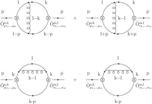
Figure 5a: The diagrams for the propagator $\langle O^{n,k}O^{m,l}\rangle^{(1)}$.

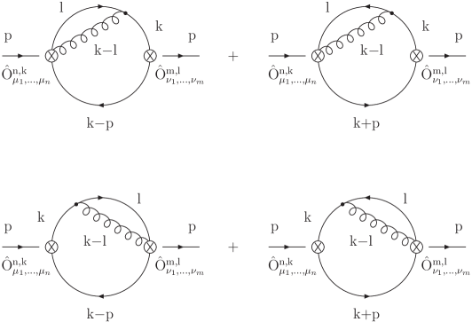
Figure 5b: The diagrams for the propagator $\langle O^{n,k}O^{m,l}\rangle^{(1)}$ (continued).

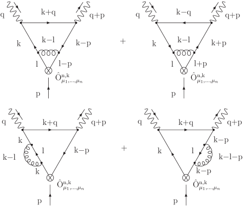
Figure 7a: The diagrams for the matrix element $\langle JJO^{n,k}\rangle^{(1)}$.

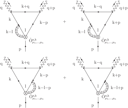
Figure 7b: The diagrams for the matrix element $\langle JJO^{n,k}\rangle^{(1)}$ (continued).

Figure 8: The diagrams which give non-leading contribution to the matrix element $\langle JJO^{n,k}\rangle^{(1)}$ at $p^{2}\rightarrow 0$.

Figure 9a: The diagrams which give contribution to the renormalization of the electromagnetic current $J^{em}$.

Figure 9b: The diagrams which give contribution to the renormalization of the electromagnetic current $J^{em}$ (continued).

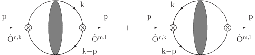
Figure 10: The diagrams which give contribution to the propagator of the composite operator in the axial gauge.

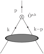
Figure 11: The diagram which describes the renormalization of the composite operator in the axial gauge.