The value of $B_{K}$ from the experimental data on CP-violation in $K$-mesons and up-to-date values of CKM matrix parameters.

Abstract

The difference between induced by box diagram quantity $\tilde{\epsilon}$ and experimentally measured value of $\epsilon$ is determined and used to obtain the value of $\tilde{\epsilon}$ with high precision. Present day knowledge of CKM matrix elements (including B-factory data), allows us to obtain from the Standard Model expression for $\tilde{\epsilon}$ the value of parameter $B_{K}$: $B_{K}=0.89\pm 0.16$. It turns out to be very close to the result of vacuum insertion, $B_{K}=1$.

1 Introduction.

It is well known that CP - violation in $K^{0}-\bar{K}^{0}$ mixing is described by the parameter $\tilde{\epsilon}$. Within the SM, this parameter is given by box diagrams. It depends in particular on the CKM matrix elements, to which vertices of box diagrams are proportional. On the other hand, the experimentally measured parameters are $\epsilon$ and $\epsilon^{\prime}$. $\epsilon$ and $\epsilon^{\prime}$ enter the measured ratios of decay amplitudes of kaons into $\pi\pi$ states. These amplitudes are superpositions of amplitudes $A(K^{0}\to(\pi\pi)_{I})=A_{I}e^{i\delta_{I}}$ of kaon decays into states with definite isospin $I=0,2$, $A_{I}$ are weak amplitudes, $\delta_{I}$ are strong rescattering phases of $\pi$-mesons. The parameter $\epsilon$ can be expressed as [1]:

$$\epsilon=\tilde{\epsilon}+i\frac{ImA_{0}}{ReA_{0}}.$$ (1)

Within the SM and in the standard parametrization of CKM matrix, $ImA_{0}$ originates from the so-called strong penguin diagrams. Amplitude $A_{2}$ also has an imaginary part which originates from electro-weak penguin diagrams. That is why $ImA_{0}>>ImA_{2}$.

Taking into account that the phases of $\epsilon$ and $\tilde{\epsilon}$ are approximately $\frac{\pi}{4}$ [1], from Eq.(1) we obtain:

$$|\tilde{\epsilon}|\approx|\epsilon|-\frac{1}{\sqrt{2}}\frac{ImA_{0}}{ReA_{0}}.$$ (2)

The estimation of $\displaystyle{\frac{ImA_{0}}{ReA_{0}}}$ was done in [2]. This term appears to be a $5-9\%$ correction to the value of $\tilde{\epsilon}$ in Eq.(2). Provided that we have estimated the right-hand side of Eq.(2) with the help of Eq.(4) we can determine parameter $B_{K}$, which parameterizes hadronic matrix element. Of course, for this purpose we need to know the values of CKM matrix elements that enter Eq.(4).

The parameters $\bar{\rho}$ and $\bar{\eta}$ of CKM matrix appear to be constrained without using the value of $\tilde{\epsilon}$ in the fit. Thus we perform the fit of CKM matrix parameters without using constraint from $\tilde{\epsilon}$ in it. Then we determine $B_{K}$ from Eqs.(2),(4). Our result is $B_{K}=0.89\pm 0.16$.

This result is close to the result of vacuum insertion: $B_{K}=1$. As discussed in [3], the insertions of $\pi$-mesons states should be taken into account. These insertions form a sign-alternating series, who’s terms depend on the cutoff momentum of $\pi$-mesons. This cutoff can be reasonably chosen to be $200-500\ MeV$ (at larger virtualities $\pi$-mesons do not exist). Then the sign-alternating series converges quickly, and one can take only first two terms. Thus taking into account the insertions of $\pi$-mesons states lowers $B_{K}$, and the agreement with our result improves further.

The lattice result of $B_{K}$ calculation is $B_{K}=0.87\pm 0.06\pm 0.14_{quench}$ [4]. We see that our result is very close to it.

The paper is organized as follows: in Section 2 we discuss various estimations of the value of $\displaystyle{\frac{ImA_{0}}{ReA_{0}}}$. In Section 3 we perform the fit of CKM matrix parameters without using constraint from $\tilde{\epsilon}$ in it. In Section 4 we determine $B_{K}$ and compare it with other results of calculation of $B_{K}$. Finally, we make our conclusion in Section 5.

2 Estimation of the numerical value of $\epsilon-\tilde{\epsilon}$.

In this section we review the estimation of $\epsilon-\tilde{\epsilon}$ [2]. We discuss the following three methods. First, one can use the experimental data on CP-violation in semileptonic $K_{L}$-decays, namely parameter $\delta_{L}$. This method possesses large uncertainty and also at the level of two sigmas contradicts the experimental value of $\displaystyle{\frac{\epsilon^{\prime}}{\epsilon}}$. Second, one can obtain the lower bound on $\epsilon-\tilde{\epsilon}$ from the experimental value of $\displaystyle{\frac{\epsilon^{\prime}}{\epsilon}}$. This lower bound is important in understanding the relative magnitude of the second term in Eq.(2), it turns out to be $\geq 5\%$. Third, we use the results of direct computation of $ImA_{0}$ in the ratio $\displaystyle{\frac{ImA_{0}}{ReA_{0}}}$, substituting the experimental value of $ReA_{0}$. This gives us a reliable estimate of $\displaystyle{\frac{ImA_{0}}{ReA_{0}}}$ with moderate error,which we use in the bulk of the paper.

First, we estimate the value of $\tilde{\epsilon}$ from the experimental results on CP-violation in semileptonic $K_{L}$ decays:

$$\delta_{L}=\frac{\Gamma(K_{L}\rightarrow l^{+}\nu\pi^{-})-\Gamma(K_{L}\rightarrow l^{-}\bar{\nu}\pi^{+})}{\Gamma(K_{L}\rightarrow l^{+}\nu\pi^{-})+\Gamma(K_{L}\rightarrow l^{-}\bar{\nu}\pi^{+})}\approx 2Re\tilde{\epsilon}.$$

$$|\tilde{\epsilon}|=\frac{\delta_{L}}{2\cos\phi},$$ (3)

where $\phi=arg(\tilde{\epsilon})$.

Now let us substitute the experimental data. For $\phi$ we use $\phi=(43.50\pm 0.05)^{\circ}$ [5]. World average value of $\delta_{L}$, published in [6], contains new KTev result: $\delta_{L}=(3.307\pm 0.063)\times 10^{-3}$. Na48 collaboration recently obtained: $\delta_{L}=(3.317\pm 0.100)\times 10^{-3}$ [7]. Averaging these two numbers we get: $\delta_{L}=(3.310\pm 0.053)\times 10^{-3}$. This leads to the following value of $\tilde{\epsilon}$:

$$|\tilde{\epsilon}|=(2.282\pm 0.037)\times 10^{-3}.$$ (4)

From Eq.(2) with the help of Eq.(2) we can find the corresponding value of $\displaystyle{\frac{ImA_{0}}{ReA_{0}}}$:

$$\frac{ImA_{0}}{ReA_{0}}=(0.03\pm 0.56)\times 10^{-4}.$$ (5)

We will show below, that this number almost contradicts the present experimental value of $\displaystyle{\frac{\epsilon^{\prime}}{\epsilon}=(1.67\pm 0.26)\times 10^{-3}}$ [5].

Second method of estimation of $\displaystyle{\frac{ImA_{0}}{ReA_{0}}}$, which gives the lower bound on it, uses the experimental value of $\displaystyle{\frac{\epsilon^{\prime}}{\epsilon}}$. The expression for $\displaystyle{\frac{\epsilon^{\prime}}{\epsilon}}$ is usually presented as follows [1]:

$$\frac{\epsilon^{\prime}}{\epsilon}=\frac{i}{\sqrt{2}}e^{i(\delta_{2}-\delta_{0})}\frac{1}{\epsilon}\left[\frac{ImA_{2}}{ReA_{0}}-w\frac{ImA_{0}}{ReA_{0}}\right]~{},$$ (6)

Let us neglect the term proportional to $ImA_{2}$ in Eq.(6), which comes from the EW penguins. Taking into account that $(\delta_{0}-\delta_{2})_{exp}=42\pm 4^{o}$ [8], we obtain the following expression for $\displaystyle{\frac{ImA_{0}}{ReA_{0}}}$ from Eq.(6):

$$\frac{ImA_{0}}{ReA_{0}}\approx-\frac{\sqrt{2}|\epsilon|}{w}\frac{\epsilon^{\prime}}{\epsilon}.$$ (7)

Substituting experimental values from [5], we get:

$$\frac{\epsilon^{\prime}}{\epsilon}=(1.67\pm 0.26)\times 10^{-3},\quad w=0.045,\quad|\epsilon|=2.284(14)\times 10^{-3}\Longrightarrow$$

$$\frac{ImA_{0}}{ReA_{0}}=-(1.2\pm 0.2)\times 10^{-4}.$$ (8)

In this way we get the following value of $|\tilde{\epsilon}|$:

$$|\tilde{\epsilon}|=2.37(2)\times 10^{-3}.$$ (9)

Since, according to Eq.(6), the contribution of EW penguins partially cancels that of QCD penguin, the value $|\displaystyle{\frac{ImA_{0}}{ReA_{0}}}|=(1.2\pm 0.2)\times 10^{-4}$ should be considered as a lower bound on $|\displaystyle{\frac{ImA_{0}}{ReA_{0}}}|$ and Eq.(9) is a lower bound on $|\tilde{\epsilon}|$. Thus the central value of $\displaystyle{\frac{ImA_{0}}{ReA_{0}}}$, obtained from semileptonic $K_{L}$-decays, Eq.(5), almost contradicts the experimental value of $\displaystyle{\frac{\epsilon^{\prime}}{\epsilon}}$.

Finally, the reliable way to estimate $\displaystyle{\frac{ImA_{0}}{ReA_{0}}}$, result of which we will use in the next sections is to use the experimental value of $ReA_{0}$ and theoretical value for $ImA_{0}$.

Calculation of $ReA_{0}$ and $ImA_{0}$, as well as $ReA_{2}$ and $ImA_{2}$, has a long history. The calculation of $ReA_{0}$ and $ReA_{2}$ was performed in order to explain the $\Delta I=\frac{1}{2}$ rule in kaon decays and the calculation of $ImA_{0}$ and $ImA_{2}$ - in order to explain the observed value of $\displaystyle{\frac{\epsilon^{\prime}}{\epsilon}}$.

In this paper we perform the calculation of $ImA_{0}$ to the following accuracy: the Wilson coefficient is calculated to LO and hadronic matrix element is calculated in naive factorization approximation. The details are presented in Appendix, and here we only quote the result:

$$\frac{ImA_{0}}{ReA_{0}}=-(3.2^{+1.1}_{-0.8})\times 10^{-4}.$$ (10)

We note that the results of computation of $ImA_{0}$ (see [9] - [14] and refs. therein) performed by a large number of people lie in the same ballpark.

Finally, from Eq.(10) we can determine the value of $\tilde{\epsilon}$:

$$|\tilde{\epsilon}|=(2.51\pm 0.07)\times 10^{-3}.$$ (11)

This number is our final result, and we will use it in Section 4.

3 Fit of the parameters of CKM matrix

We use in our fit of the CKM matrix experimentally measured values of modulus of matrix elements $V_{ud}$,$V_{us}$,$V_{ub}$,$V_{cd}$,$V_{cs}$, $V_{cb}$ and also $sin2\alpha$, $sin2\beta$, $sin2\gamma$ and $\Delta m_{B_{d}}$. Note that we do not use $\tilde{\epsilon}$ in fit, since we plan to determine the value of $B_{K}$ with the help of the fit results.

We assume these experimentally measured data to be normally distributed. Also the theoretical uncertainties are treated as normally distributed. Let us note that other people treat theoretical uncertainties in other way [16], [17].

The table of input parameters looks like:

Parameter	Value	Standard Deviation
$|V_{ud}|\cite[cite]{[\@@bibref{}{PDG}{}{}]}$	0.9738	0.0005
$|V_{us}|\cite[cite]{[\@@bibref{}{PDG}{}{}]}$	0.2200	0.0026
$|V_{ub}|\cite[cite]{[\@@bibref{}{PDG}{}{}]}$	0.00367	0.00047
$|V_{cd}|\cite[cite]{[\@@bibref{}{PDG}{}{}]}$	0.224	0.012
$|V_{cs}|\cite[cite]{[\@@bibref{}{PDG}{}{}]}$	0.996	0.013
$|V_{cb}|\cite[cite]{[\@@bibref{}{PDG}{}{}]}$	0.0413	0.0015
$sin2\alpha$ [18]	-0.21	0.46
$sin2\beta$ [5]	0.736	0.049
$sin2\gamma$ [19]	0.69	0.58

The $\chi^{2}$ expression which we minimize looks like:

$$\chi^{2}(A,\lambda,\bar{\rho},\bar{\eta})=\left(\frac{V^{theo}_{ud}-V^{exp}_{ud}}{\sigma_{V_{ud}}}\right)^{2}+\left(\frac{V^{theo}_{us}-V^{exp}_{us}}{\sigma_{V_{us}}}\right)^{2}+\left(\frac{V^{theo}_{ub}-V^{exp}_{ub}}{\sigma_{V_{ub}}}\right)^{2}+\left(\frac{V^{theo}_{cd}-V^{exp}_{cd}}{\sigma_{V_{cd}}}\right)^{2}+$$

$$+\left(\frac{V^{theo}_{cs}-V^{exp}_{cs}}{\sigma_{V_{cs}}}\right)^{2}+\left(\frac{V^{theo}_{cb}-V^{exp}_{cb}}{\sigma_{V_{cb}}}\right)^{2}+\left(\frac{\Delta m^{theo}_{B_{d}}-\Delta m^{exp}_{B_{d}}}{\sigma_{\Delta_{m}}}\right)^{2}+\left(\frac{sin2\alpha^{theo}-sin2\alpha^{exp}}{\sigma_{sin2\alpha}}\right)^{2}+$$

$$+\left(\frac{sin2\beta^{theo}-sin2\beta^{exp}}{\sigma_{sin2\beta}}\right)^{2}+\left(\frac{sin2\gamma^{theo}-sin2\gamma^{exp}}{\sigma_{sin2\gamma}}\right)^{2},$$ (12)

where theoretical expressions depend on four Wolfenstein parameters: $A$, $\lambda$, $\bar{\rho}$ and $\bar{\eta}$. Expression (3) was minimized varying them.

Here are our results:

$$\lambda=0.224\pm 0.002\qquad\qquad\alpha^{[deg]}=100\pm 5$$

$$A=0.82\pm 0.03\qquad\qquad\beta^{[deg]}=23\pm 2$$

$$\bar{\rho}=0.22\pm 0.04\qquad\qquad\gamma^{[deg]}=57\pm 5$$

$$\bar{\eta}=0.34\pm 0.02\qquad\qquad\hskip 48.0pt$$

$$\chi^{2}/n.d.o.f.=8.1/5\;\;.$$

For comparison, we present the results of the fit, made by CKMfitter Group [16] and UTfit Collaboration [17]:

	CKMfitter	UTfit
$\lambda$	$0.226\pm 0.002$	$0.226\pm 0.002$
$A$	$0.80^{+0.03}_{-0.02}$
$\bar{\rho}$	$0.19^{+0.09}_{-0.07}$	$0.17\pm 0.05$
$\bar{\eta}$	$0.36^{+0.05}_{-0.04}$	$0.35\pm 0.03$

	CKMfitter	UTfit
$\alpha^{[deg]}$	$94^{+12}_{-10}$	$94\pm 8$
$\beta^{[deg]}$	$23.8^{+2.1}_{-2.0}$	$23.2\pm 1.4$
$\gamma^{[deg]}$	$62^{+10}_{-12}$	$61.6\pm 7$

4 The value of $B_{K}$

From the results of the fit, presented above, we can extract the value of $B_{K}$. For this purpose we use the theoretical expression for $|\tilde{\epsilon}|$, first obtained in [20]. It has the following form:

$$|\tilde{\epsilon}^{theo}|=\frac{G^{2}_{F}m_{K}f^{2}_{K}}{12\sqrt{2}\pi^{2}\Delta m_{K}}B_{K}(\eta_{cc}m_{c}^{2}Im[(V_{cs}V^{*}_{cd})^{2}]+\eta_{tt}m_{t}^{2}I(\xi)Im[(V_{ts}V^{*}_{td})^{2}]$$

$$+2\eta_{ct}m_{c}^{2}\ln(\frac{m_{W}^{2}}{m_{c}^{2}})Im[V_{cs}V^{*}_{cd}V_{ts}V^{*}_{td}]).$$ (13)

Here $\displaystyle{I(\xi)=\{\frac{\xi^{2}-11\xi+4}{4(\xi-1)^{2}}-\frac{3\xi^{2}\ln\xi}{2(1-\xi)^{3}}\}}$, $\xi=m^{2}_{t}/m^{2}_{W}$. Quark masses are $m_{c}=1.2\pm 0.2$ GeV [5], $m_{t}=178.0\pm 4.3$ GeV [21], $m_{W}=80.42\pm 0.04$ GeV [5]. The QCD corrections were calculated to leading order in [20]: $\eta_{cc}=0.6$, $\eta_{tt}=0.6$, $\eta_{ct}=0.4$. The next-to-leading order calculation changes slightly $\eta_{tt}$ and $\eta_{ct}$ and changes considerably $\eta_{cc}$: $\eta_{cc}=1.32\pm 0.32$ [22], $\eta_{tt}=0.574\pm 0.01$ [23], $\eta_{ct}=0.47\pm 0.04$ [24]. The kaon decay constant extracted from the $K^{+}\rightarrow\mu^{+}\nu$ decay width equals: $f_{K}=160.4\pm 1.9$ MeV [5]. The $K_{L}-K_{S}$ mass difference is $\Delta m_{K}=(3.483\pm 0.006)\times 10^{-15}$ GeV [5]. Fermi constant $G_{F}=1.16639(1)\times 10^{-5}GeV^{-2}$[5].

Now we equate this expression to the value of $|\tilde{\epsilon}|=(2.51\pm 0.07)\times 10^{-3}$ from Eq.(11), substituting all experimental numbers and the results of the fit. This leads to the following value of $B_{K}$:

$$B_{K}=0.89\pm 0.16$$ (14)

Note that it is close to the result of vacuum insertion: $B_{K}=1$.

5 Conclusions

We have extracted the value of $B_{K}$ using the fitted values of CKM matrix elements and the estimated difference between $\tilde{\epsilon}$ and $\epsilon$. Our result is $B_{K}=0.89\pm 0.16$. It appears to be close to the result of vacuum insertion, $B_{K}=1$, while lattice result is simply the same: $B_{K}=0.87\pm 0.06\pm 0.14_{quench}$ [4].

Appendix A Estimation of the value of $ImA_{0}$ from QCD penguin diagram.

Let’s estimate $\frac{ImA_{0}}{ReA_{0}}$, using experimental value of $ReA_{0}$ and evaluating the value of $ImA_{0}$. The latter will be evaluated to the following accuracy: the LO Wilson coefficients will be used, and hadronic matrix element will be calculated in naive factorization approximation.

As it is well known transitions with $\Delta S=1$ are due to the 4-quark effective Hamiltonian, for the first time derived in [25]:

$$H_{\Delta S=1}=\sqrt{2}G_{F}\sin\theta_{C}\cos\theta_{C}\sum_{i=1}^{6}c_{i}O_{i}$$ (15)

The so-called penguin operator $O_{5}$ dominates in amplitudes $K^{0}\rightarrow(\pi\pi)_{I=0}$ [25]:

$$O_{5}=\bar{s}_{L}\gamma_{\mu}\lambda^{a}d_{L}(\bar{u}_{R}\gamma_{\mu}\lambda^{a}u_{R}+\bar{d}_{R}\gamma_{\mu}\lambda^{a}d_{R})$$ (16)

Below we present the detailed derivation of the coefficient function $c_{5}$ in one loop approximation.

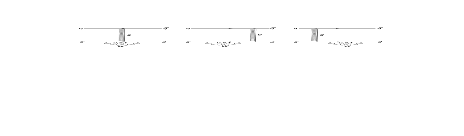
Figure 1: Diagrams, which contribute to the penguin operator.

It is convenient to perform calculation in the unitary gauge. Each of the three diagrams (see Fig. 1) is infinite, however the sum appears to be finite. We will use the dimensional regularization ($d=4-2\epsilon$), in order to regularize divergent integrals:

$$M_{0}=\frac{g^{2}g_{s}^{2}}{2}\frac{1}{q^{2}}\sum_{j=u,c,t}\int\frac{d^{d}k}{(2\pi)^{d}}\frac{g_{\mu\nu}-\frac{k_{\mu}k_{\nu}}{M_{W}^{2}}}{k^{2}-M_{W}^{2}}\bar{s}_{L}\gamma_{\mu}\frac{1}{\hat{q}_{2}-m_{j}}\gamma_{\rho}\frac{\lambda_{a}}{2}\frac{1}{\hat{q}_{1}-m_{j}}\gamma_{\nu}d_{L}\left(\bar{\psi}_{r}\gamma_{\rho}\frac{\lambda_{a}}{2}\psi_{r}\right)V_{jd}V_{js}^{*},$$

$$M_{1}=\frac{g^{2}g_{s}^{2}}{2}\frac{1}{q^{2}}\sum_{j=u,c,t}\int\frac{d^{d}k}{(2\pi)^{d}}\frac{g_{\mu\nu}-\frac{k_{\mu}k_{\nu}}{M_{W}^{2}}}{k^{2}-M_{W}^{2}}\bar{s}\gamma_{\mu}p_{L}\frac{1}{\hat{q}_{2}-m_{j}}\gamma_{\nu}p_{L}\frac{1}{\hat{p}_{2}-m_{j}}\gamma_{\rho}\frac{\lambda_{a}}{2}d\left(\bar{\psi}_{r}\gamma_{\rho}\frac{\lambda_{a}}{2}\psi_{r}\right)V_{jd}V_{js}^{*},$$

$$M_{2}=\frac{g^{2}g_{s}^{2}}{2}\frac{1}{q^{2}}\sum_{j=u,c,t}\int\frac{d^{d}k}{(2\pi)^{d}}\frac{g_{\mu\nu}-\frac{k_{\mu}k_{\nu}}{M_{W}^{2}}}{k^{2}-M_{W}^{2}}\bar{s}\gamma_{\rho}\frac{\lambda_{a}}{2}\frac{1}{\hat{p}_{1}-m_{j}}\gamma_{\mu}p_{L}\frac{1}{\hat{q}_{1}-m_{j}}\gamma_{\nu}p_{L}d\left(\bar{\psi}_{r}\gamma_{\rho}\frac{\lambda_{a}}{2}\psi_{r}\right)V_{jd}V_{js}^{*},$$

$$M=M_{0}+M_{1}+M_{2}.$$ (17)

The effective Hamiltonian is equal to:

$$H_{penguin}=iM.$$ (18)

The result of the calculation can be presented in the following form:

$$H_{penguin}=-\sum_{j=u,c,t}\frac{g^{2}g_{s}^{2}}{48\pi^{2}}\frac{1}{q^{2}}\bar{s}_{L}G_{\rho}(q)\frac{\lambda_{a}}{2}d_{L}\left(\bar{\psi}_{r}\gamma_{\rho}\frac{\lambda_{a}}{2}\psi_{r}\right)V_{jd}V_{js}^{*},$$

$$G_{\rho}=G_{1}\gamma_{\rho}+\frac{1}{M_{W}^{2}}\left(G_{2}\hat{p}_{2}\gamma_{\rho}\hat{p}_{1}+G_{3}\hat{p}_{1}p_{1\rho}+G_{4}\hat{p}_{2}p_{2\rho}+G_{5}\hat{p}_{1}p_{2\rho}+G_{6}\hat{p}_{2}p_{1\rho}\right).$$ (19)

Dimensionless functions $G_{i}$ ($i=1,2,3,4,5,6$) depend on the values $x_{j}=\frac{m_{j}^{2}}{M_{W}^{2}}$, $q^{2}$, $m_{s}^{2}$, $m_{d}^{2}$, where $m_{j}$ is the up-quark mass in the loop. We suppose the external $s$ and $d$ quarks to be on mass shell.

Let us neglect d-quark mass. In this approximation the non-zero contribution into operator $H_{penguin}$ is given by the terms with formfactors $G_{1},G_{4}$ and $G_{6}$. It is convenient to introduce new variables $P=p_{1}+p_{2}$ and $q=p_{1}-p_{2}$:

$$\bar{s}_{L}G_{\rho}\frac{\lambda_{a}}{2}d_{L}=G_{1}\bar{s}_{L}\gamma_{\rho}\frac{\lambda_{a}}{2}d_{L}+\frac{m_{s}\left((G_{6}+G_{4})P_{\rho}+(G_{6}-G_{4})q_{\rho}\right)}{2M_{W}^{2}}\bar{s}_{R}\frac{\lambda_{a}}{2}d_{L}.$$ (20)

Here the term proportional to $q_{\rho}$ will not contribute to operator $H_{penguin}$, since $q_{\rho}\times\left(\bar{\psi}_{r}\gamma_{\rho}\frac{\lambda_{a}}{2}\psi_{r}\right)=(m_{r}-m_{r})\left(\bar{\psi}_{2}\frac{\lambda_{a}}{2}\psi_{1}\right)=0$. The quantity $P_{\rho}\bar{s}_{R}\frac{\lambda_{a}}{2}d_{L}$ should be expressed through the magnetic formfactor with the help of the following equation:

$$\bar{s}\sigma_{\mu\nu}q_{\nu}\frac{\lambda_{a}}{2}d_{L}=\frac{i}{2}q_{\nu}\bar{s}(\gamma_{\mu}\gamma_{\nu}-\gamma_{\nu}\gamma_{\mu})\frac{\lambda_{a}}{2}d_{L}=i(m_{s}\bar{s}_{L}\gamma_{\mu}\frac{\lambda_{a}}{2}d_{L}-P_{\mu}\bar{s}_{R}\frac{\lambda_{a}}{2}d_{L}).$$ (21)

With the help of Eq.(21) from Eq.(20) we obtain:

$$H_{penguin}=-\sum_{j=u,c,t}\frac{g^{2}g_{s}^{2}}{48\pi^{2}}\frac{1}{q^{2}}\left(f_{1}\bar{s}_{L}\gamma_{\mu}\frac{\lambda_{a}}{2}d_{L}+i\frac{f_{2}}{M_{W}^{2}}m_{s}q_{\nu}\bar{s}_{R}\sigma_{\mu\nu}\frac{\lambda_{a}}{2}d_{L}\right)\bar{\psi}_{r}\gamma_{\mu}\frac{\lambda_{a}}{2}\psi_{r}V_{jd}V_{js}^{*},$$ (22)

where $f_{1}$ and $f_{2}$ are equal to:

$$f_{1}=G_{1}+\frac{m_{s}^{2}}{2M_{W}^{2}}(G_{6}+G_{4}),$$

$$f_{2}=\frac{G_{6}+G_{4}}{2}.$$ (23)

It is sufficient to calculate the formfactors $G_{4}$ and $G_{6}$ in the zero order in $q^{2}$, $m_{s}^{2}$. However, the formfactor $G_{1}$, as it follows from last equations, should be calculated, including terms proportional to $m_{s}^{2}$, $q^{2}$. From equations (A), calculating appropriate integrals, we get:

$$G_{1}=R_{1}\frac{q^{2}}{M_{W}^{2}}+R_{2}\frac{m_{s}^{2}}{M_{W}^{2}},$$

$$R_{1}=\frac{7x^{4}+14x^{3}-63x^{2}+38x+4+6(16x-9x^{2}-4)\ln x}{24(1-x)^{4}},$$

$$R_{2}=\frac{-5x^{4}+14x^{3}-39x^{2}+38x-8+18x^{2}\ln x}{8(1-x)^{4}},$$

$$G_{4}=\frac{2x^{4}-14x^{3}+45x^{2}-38x+5+6(1-4x)\ln x}{6(1-x)^{4}},$$

$$G_{6}=\frac{11x^{4}-14x^{3}+27x^{2}-38x+14+6(8x-9x^{2}-2)\ln x}{12(1-x)^{4}}.$$ (24)

Substituting these formulas into equations (A), we obtain:

$$f_{1}=\frac{7x^{4}+14x^{3}-63x^{2}+38x+4+6(16x-9x^{2}-4)\ln x}{24(1-x)^{4}}\frac{q^{2}}{M_{W}^{2}},$$

$$f_{2}=\frac{5x^{4}-14x^{3}+39x^{2}-38x+8-18x^{2}\ln x}{8(1-x)^{4}}.$$ (25)

Finally, let us rewrite equation (22) in the following way:

$$H_{penguin}=-\sum_{j=u,c,t}\frac{g^{2}g_{s}^{2}}{48\pi^{2}M_{W}^{2}}\left(F_{1}\bar{s}_{L}\gamma_{\mu}\frac{\lambda_{a}}{2}d_{L}+iF_{2}m_{s}\frac{q_{\nu}}{q^{2}}\bar{s}_{R}\sigma_{\mu\nu}\frac{\lambda_{a}}{2}d_{L}\right)\bar{\psi}_{r}\gamma_{\mu}\frac{\lambda_{a}}{2}\psi_{r}V_{jd}V_{js}^{*},$$

$$F_{1}=\frac{7x^{4}+14x^{3}-63x^{2}+38x+4+6(16x-9x^{2}-4)\ln x}{24(1-x)^{4}},$$

$$F_{2}=f_{2}=\frac{5x^{4}-14x^{3}+39x^{2}-38x+8-18x^{2}\ln x}{8(1-x)^{4}}.$$ (26)

As the admixture of gluons in $K$ and $\pi$ mesons is small, the contribution of magnetic moment operator in (A) is negligible [25].

Substituting $m_{c}=1.2$ GeV, $m_{t}=178.0$ GeV, $M_{W}=80.42$ GeV for the formfactor $F_{1}$ we obtain:

$$F_{1}(x<<1)\approx-\ln x+\frac{1}{6},$$

$$F_{1}(x_{c})\approx 8.58,$$

$$F_{1}(x_{t})\approx 0.550,$$

$$F_{1}(\infty)=\frac{7}{24}\approx 0.292.$$ (27)

Formula (A) can be rewritten with good accuracy as:

$$H_{penguin}\approx\sqrt{2}G_{F}\sin{\theta_{C}}\cos{\theta_{C}}\left(-\frac{\alpha_{s}}{12\pi}\ln\frac{m_{c}^{2}}{\mu^{2}}+i\frac{ImV_{cd}V_{cs}^{*}}{ReV_{cd}V_{cs}^{*}}\frac{\alpha_{s}}{12\pi}\ln\frac{M_{W}^{2}}{m_{c}^{2}}\right)O_{5},$$ (28)

where instead of $m_{u}$ the characteristic hadronic scale $\mu$ (this time “low” normalization point) is substituted.

Thus the real and imaginary parts of $c_{5}$ are equal to:

$$Rec_{5}=-\frac{\alpha_{s}}{12\pi}\ln\frac{m_{c}^{2}}{\mu^{2}}$$

$$Imc_{5}=\frac{ImV_{cd}V_{cs}^{*}}{ReV_{cd}V_{cs}^{*}}\frac{\alpha_{s}}{12\pi}\ln\frac{M_{W}^{2}}{m_{c}^{2}}.$$ (29)

In order to understand at which virtuality $\alpha_{s}$ should be taken in these expressions leading logarithms should be summed up. This was done for the real part of coefficient function in the paper [25]:

$$Rec_{5}=\left(\chi_{1}^{0.48}\left(-0.039\,\chi_{2}^{0.8}+0.033\,\chi_{2}^{0.42}+0.003\,\chi_{2}^{-0.12}+0.003\,\chi_{2}^{-0.3}\right)+\right.$$

$$\left.+\chi_{1}^{-0.24}\left(-0.014\,\chi_{2}^{0.8}-0.001\,\chi_{2}^{0.42}-0.014\,\chi_{2}^{-0.12}+0.029\,\chi_{2}^{-0.3}\right)\right),$$ (30)

while for imaginary part in paper [26] the following result was obtained:

$$Imc_{5}=\frac{ImV_{cd}V_{cs}^{*}}{ReV_{cd}V_{cs}^{*}}\left(0.0494\,\chi_{1}^{0.85}-0.0280\,\chi_{1}^{0.42}+0.0116\,\chi_{1}^{-0.13}-0.0330\,\chi_{1}^{-0.35}\right)\times$$

$$\times\left(0.8509\,\chi_{2}^{0.8}+0.0091\,\chi_{2}^{0.42}+0.1222\,\chi_{2}^{-0.12}+0.0178\,\chi_{2}^{-0.3}\right),$$ (31)

where $\chi_{1}=\frac{\alpha_{s}(m_{c})}{\alpha_{s}(m_{W})}$, $\chi_{2}=\frac{\alpha_{s}(\mu)}{\alpha_{s}(m_{c})}$.

12pt

Numerical analysis shows that with a good accuracy expression for $Rec_{5}$ can be written as:

$$Rec_{5}=-\frac{\alpha_{s}(\mu)}{12\pi}\log(\frac{m_{c}^{2}}{\mu^{2}}).$$ (32)

On the other hand $Imc_{5}$ at the scale $\mu$ at which $\alpha_{s}(\mu)=1$ has the value

$$Imc_{5}=\frac{ImV_{cd}V_{cs}^{*}}{ReV_{cd}V_{cs}^{*}}\times 0.13.$$ (33)

The expression for $ImA_{0}$ can be written as:

$$ImA_{0}=\sqrt{2}G_{F}\sin\theta_{C}\cos\theta_{C}Im(c_{5})<(\pi\pi)_{I=0}|O_{5}|K^{0}>$$ (34)

In order to get the value of $ImA_{0}$ we must calculate hadronic matrix element of penguin operator. It was evaluated in the framework of naive quark model in [25], see also [27]:

$$<(\pi\pi)_{I=0}|O_{5}|K^{0}>=\frac{4\sqrt{6}}{9}\frac{m_{K}^{2}m_{\pi}^{2}f_{\pi}}{m_{s}(m_{u}+m_{d})}\left(\frac{f_{K}}{f_{\pi}}(1+\frac{m_{K}^{2}}{m_{\sigma}^{2}})-1\right)$$ (35)

Substituting experimental numbers $G_{F}=1.166\times 10^{-5}GeV,\sin\theta_{C}=0.22,\cos\theta_{C}=0.95,m_{\pi}=135MeV,m_{K}=497MeV,f_{\pi}=130MeV,f_{K}=160MeV,m_{\sigma}=700MeV$ and quark masses $m_{s}=130MeV,m_{u}=3MeV,m_{d}=7MeV$, we get:

$$ImA_{0}=-1.1\times 10^{-10}GeV.$$ (36)

Finally, dividing it by experimentally measured $ReA_{0}=3.33\times 10^{-7}GeV$, we obtain:

$$\frac{ImA_{0}}{ReA_{0}}=-3.2\times 10^{-4}.$$ (37)

In order to estimate the theoretical error for $ImA_{0}$ we propose the following method: to take two values of $\mu$, corresponding to $\alpha_{s}(\mu)=\frac{2}{3}$ and $\alpha_{s}(\mu)=\frac{3}{2}$, to calculate $\frac{ImA_{0}}{ReA_{0}}$ at each $\mu$ and from these boundary values get $\pm$ error for $\frac{ImA_{0}}{ReA_{0}}$.

Via the proposed method we get our final result:

$$\frac{ImA_{0}}{ReA_{0}}=-(3.2^{+1.1}_{-0.8})\times 10^{-4}.$$ (38)

This number is rather stable with respect to the variation of $\mu$. Our result confirms statement maid in [27]: QCD penguin results in the value of $\displaystyle{\frac{\epsilon^{\prime}}{\epsilon}}$ in ballpark of the experimental data.

On the other hand the real part is very sensitive to $\mu$, as can be seen from Eq.(32). The expression for $ReA_{0}$ has the following form:

$$ReA_{0}=\sqrt{2}G_{F}\sin\theta_{C}\cos\theta_{C}Re(c_{5})<(\pi\pi)_{I=0}|O_{5}|K^{0}>.$$ (39)

Substituting numbers and again taking $\mu$ at which $\alpha_{s}(\mu)=\frac{2}{3}$ and $\alpha_{s}(\mu)=\frac{3}{2}$ we get: $ReA_{0}=(1.2^{+0.8}_{-0.6})\times 10^{-7}GeV$. The central number is approximately 3 times smaller than the experimental , but theoretical uncertainty is large.