Gaps between Jets in the High Energy Limit

Abstract:

We use perturbative QCD to calculate the parton level cross section for the production of two jets that are far apart in rapidity, subject to a limitation on the total transverse momentum $Q_{0}$ in the interjet region. We specifically address the question of how to combine the approach which sums all leading logarithms in $Q/Q_{0}$ (where $Q$ is the jet transverse momentum) with the BFKL approach, in which leading logarithms of the scattering energy are summed. This paper constitutes progress towards the simultaneous summation of all important logarithms. Using an “all orders” matching, we are able to obtain results for the cross section which correctly reproduce the two approaches in the appropriate limits.

1 Introduction

Events with high-$p_{T}$ jets separated by large rapidity gaps at hadron colliders are of significant theoretical interest. Studying these events provides us with the possibility to better understand QCD in the high energy limit and also to understand QCD radiation in “gap” events. There are two major approaches to the production of two gap-separated jets.

In the first approach, parton-parton elastic scattering with a QCD colour singlet exchange is regarded as providing the leading contribution to the cross-section. The leading-$Y$ terms ($Y$ is the rapidity interval between the jets) are summed, i.e.

$$\sim\alpha_{s}^{n}Y^{n}$$ (1)

This is the so-called BFKL [1] approach to the gaps between jets process. The observable calculated in this approach does not consider any radiation into the interjet region. Experiments though, impose an upper bound on this radiation by necessity. Calculations [2, 3, 4, 5, 6] based on this approach have been performed and compared with some success to the data from HERA and Tevatron [7].

In the second approach the energy flow into the gap is certainly considered. In accord with experimental observations soft radiation with transverse energy below $Q_{0}$ is allowed in the interjet region. This gives rise to logarithms of $Q/Q_{0}$ where $Q$ is the transverse momentum of the jets. The aim here is to sum all terms of the form

$$\sim\alpha_{s}^{n}Y^{m}L^{n}\;,\quad m\leq n$$ (2)

where $L=\ln Q^{2}/Q_{0}^{2}$. In particular, at each order of $\alpha_{s}$ the full $Y$-dependence of the coefficient of $L^{n}$ is kept. The global leading logarithms of $Q/Q_{0}$ ($LLQ_{0}$) have been summed for various jet definitions [8, 9, 10, 11] and non-global effects have been considered in [11, 12].

For asymptotically large $Y$ at fixed $L$ the BFKL approach is expected to be the most appropriate one. On the other hand, using a gap definition with large values of $Q_{0}$ at realistic collider energies the second approach ought to be the best. In order to get a better understanding of the gaps-between-jets processes at colliders it is desirable to combine the two approaches. This is the main issue of this paper.

To combine the two approaches order-by-order we need to prevent double counting and make sure the divergences arising from the BFKL approach (at each order in $\alpha_{s}$) cancel in the jet cross section. To this end we recalculate the gap cross section with limited transverse energy-flow into the gap in the high energy limit. In addition to the double-leading-logarithmic ($DLL$) terms we also consider certain terms sub-leading in $Y$, namely those arising from the imaginary parts of the loop integrals. In the first instance, we thus sum terms of the type

$$\sim\alpha_{s}^{n}L^{n}Y^{m}\pi^{n-m}\;,\quad m\leq n$$ (3)

where only integer powers of $\pi^{2}$ appear. We term this approximation the $\pi^{2}DLLA$ . We argue that the gap cross section can be obtained by calculating the elastic quark-quark amplitude with all virtual gluon rapidities constrained to the gap region and all transverse momenta constrained to be above $Q_{0}$. Based on this we show that in the $\pi^{2}DLLA$ , and also in the $LLQ_{0}A$, the BFKL cross section can be included explicitly up to $\mathcal{O}(\alpha_{s}^{5})$ and derive the expression for the combined gap cross section.

At this stage, we have not been able to go beyond $\mathcal{O}(\alpha_{s}^{5})$ in fixed-order matching. However, we do present an all-orders cross section that smoothly interpolates between the $LLQ_{0}$ and the BFKL results. In this context, we consider three phenomenological matching schemes.

The remainder of the paper is structured as follows. In the next section we calculate the gap cross section in the $\pi^{2}DLLA$ , consider some approximations to it and compare to the $LLQ_{0}$ cross section. Then, we calculate the quark-quark scattering amplitude in the leading-$Y$ (BFKL) approximation, deriving the general result at any fixed order in $\alpha_{s}$. Finally we discuss the matching of the two approaches. Firstly we attempt a fixed-order matching which we are able to accomplish to $\mathcal{O}(\alpha_{s}^{5})$ and then we present our all-order matching results.

2 Summing logarithms in $Q_{0}$

We seek to calculate the cross section for two-jet production in the high-energy (i.e. high rapidity separation) limit, with limited total scalar transverse momentum in the interjet region. We require this transverse momentum to be below $Q_{0}$, the jets to have transverse momentum $Q$, and be separated by a rapidity interval $Y$, and consider the region

$$\Lambda_{QCD}^{2}\ll Q_{0}^{2}\ll Q^{2}\ll\hat{s}=\mathrm{e}^{Y}\,Q^{2}.$$ (4)

The first of these relations is to ensure that we can use perturbation theory, although we will ultimately be interested in extrapolating $Q_{0}$ towards $\Lambda_{QCD}$, while the other two are to ensure that the logarithms we are interested in are large. In this section, we calculate the partonic gap cross section for the process, $\mathrm{qq^{\prime}\to qq^{\prime}}$

$$\sigma\equiv\frac{\mathrm{d}\sigma(\hat{s},Q_{0},Y)}{\mathrm{d}Q^{2}}$$ (5)

for fixed $\hat{s}$ in the $\pi^{2}DLLA$ . Since we are not sensitive to collinear emission, we do not need to worry about the details of initial state collinear factorization, and only calculate partonic cross sections.

Our approximation implies the eikonal (soft gluon) approximation, valid when $Q^{2}\ll\hat{s}$. To generate the leading logs in $Q_{0}$, we make the approximation of strongly-ordered transverse momenta for the real and virtual gluons. The scalar sum of all gluon transverse momenta can therefore be approximated by the largest single transverse momentum, $\sum_{i}q_{\perp i}\approx\max_{i}q_{\perp i}$. We therefore require that any real gluon emitted in the gap region have transverse momentum below $Q_{0}$.

Let us denote denote by $\sigma^{(n)}$ the gap cross section at $\mathcal{O}(\alpha_{s}^{n+2})$. Clearly at zeroth order, the gap cross section coincides with the inclusive cross section,

$$\sigma^{(0)}=\frac{4\pi\alpha_{s}^{2}}{Q^{4}}\frac{(N_{c}^{2}-1)}{4N_{c}^{2}}.$$ (6)

As the basis for the calculation to all orders we employ the following theorem.

2.1 Theorem

“At any finite order in perturbation theory, in the strongly-ordered approximation, the gap cross section is given by the two-to-two cross section, with all virtual gluon rapidities constrained to the gap region and transverse momenta above $Q_{0}$, and with the exchanged gluons attached only to the external lines.”

This is clearly a major simplification, since it means we never have to calculate any real emission or triple-gluon-vertex diagrams.

Central to the proof of this theorem is the following result. For every cut through a given cut diagram, and every way of attaching a softer gluon to the external lines of that diagram, we can always make four cuts: in which the soft gluon is to the left of the cut; to the right of the cut; crossing the cut from left to right; and crossing the cut from right to left. The contributions from the real parts of the loop integral are equal and opposite to the real emission integral. The imaginary part of the loop integral, if present, cancels between the cuts to the left and right of the gluon. The total contributions are therefore equal and opposite.

It is then straightforward to see that we only get a non-zero contribution from configurations in which all gluons, real or virtual, have transverse momentum above $Q_{0}$. If the softest gluon is below $Q_{0}$, then the value of the observable is the same, whether it is real or virtual. The cancellation is therefore able to take place and we get zero contribution. Therefore the softest gluon must be above $Q_{0}$, therefore all gluons must be above $Q_{0}$.

We can also use the same argument to prove that the softest gluon must be within the gap region. The same argument does not however apply to harder gluons, as it is not guaranteed that for them all four cuts listed above are consistent with strong ordering. We assume here, as in conventional calculations of gaps-between-jets processes, that contributions from outside the gap region cancel, but note that our recent work has cast doubt on this assumption [13]. Therefore, all gluons must be within the gap region. Finally, since for a real gluon in the gap region our observable is zero, all gluons must be virtual.

2.2 Calculation in the $\pi^{2}DLLA$

We therefore have to calculate the all-orders amplitude for quark $2\to 2$ scattering, with the phase space for the gluons constrained to the gap region in rapidity and with transverse momentum above $Q_{0}$. The loop integrals themselves are trivial – they are just nested sets of integrals. The only complication concerns the colour structure.

Let us denote by $\mathcal{A}\mathbf{C}(Q_{0})$ the amplitude defined above, including its colour factor. It can be decomposed into singlet and octet components,

$$\mathcal{A}\mathbf{C}(Q_{0})=\mathcal{A}_{1}(Q_{0})\,\mathbf{C}_{1}+\mathcal{A}_{8}(Q_{0})\,\mathbf{C}_{8}.$$ (7)

The gap cross section we are interested in is therefore proportional to

$$\sigma\propto|\mathcal{A}_{1}(Q_{0})|^{2}\mathrm{Tr}\{\mathbf{C}_{1}^{\dagger}\mathbf{C}_{1}\}+|\mathcal{A}_{8}(Q_{0})|^{2}\mathrm{Tr}\{\mathbf{C}_{8}^{\dagger}\mathbf{C}_{8}\}=|\mathcal{A}_{1}(Q_{0})|^{2}N_{c}^{2}+|\mathcal{A}_{8}(Q_{0})|^{2}\frac{1}{4}(N_{c}^{2}-1).$$ (8)

We denote the $n$th order contribution to the colour amplitudes as $\mathcal{A}_{i}^{(n)}$. Since for $Q_{0}=Q$ the transverse momentum integrals give zero, we must have

$$\mathcal{A}_{i}(Q)=\mathcal{A}_{i}^{(0)}.$$ (9)

Since the zeroth order contributions $\mathcal{A}_{i}^{(0)}$ are given by single gluon exchange, we have $\mathcal{A}_{1}^{(0)}=0$. We choose to normalize $\mathcal{A}_{8}^{(0)}$ in such a way that the constant of proportionality in (8) is unity, i.e.

$$\mathcal{A}_{8}^{(0)}=\sqrt{\frac{\sigma^{(0)}}{\frac{1}{4}(N_{c}^{2}-1)}}.$$ (10)

We introduce a simple vector notation, with basis vectors $\underline{e}_{1}=\mathbf{C}_{1}$ and $\underline{e}_{2}=\mathbf{C}_{8}$, such that

$$\underline{\mathcal{A}}=\left(\begin{array}[]{c}\mathcal{A}_{1}\\ \mathcal{A}_{8}\end{array}\right),$$ (11)

and we can write

$$\sigma=\underline{\mathcal{A}}^{\dagger}(Q_{0})\,\mathrm{S}\,\underline{\mathcal{A}}(Q_{0}),$$ (12)

with

$$\mathrm{S}=\left(\begin{array}[]{cc}N_{c}^{2}&0\\ 0&\frac{1}{4}(N_{c}^{2}-1)\end{array}\right).$$ (13)

We explicitly calculate the amplitude at $\mathcal{O}(\alpha_{s}^{2})$ and $\mathcal{O}(\alpha_{s}^{3})$. Note that, besides the (real) leading-$Y$ parts of the amplitudes we also keep the sub-leading terms which differ from the leading parts in the powers of $Y$ and $\pi$, see appendix. As for the one-loop amplitude $\underline{\mathcal{A}}^{(1)}(Q_{0})$ the soft gluon exchange changes the colour of the external quarks, so that the one-loop correction can be considered to be a matrix acting on $\underline{\mathcal{A}}^{(0)}$ to obtain $\underline{\mathcal{A}}^{(1)}$. Similarly, $\underline{\mathcal{A}}^{(2)}$ can be obtained from $\underline{\mathcal{A}}^{(1)}$. We can therefore write the result in matrix form as

$$\underline{\mathcal{A}}^{(1)}(Q_{0})=-\frac{2\alpha_{s}}{\pi}\int_{Q_{0}}^{Q}\frac{\mathrm{d}k_{\perp}}{k_{\perp}}\Gamma\,\underline{\mathcal{A}}^{(0)},$$ (14)

and

$$\underline{\mathcal{A}}^{(2)}(Q_{0}) = \left(\frac{2\alpha_{s}}{\pi}\right)^{2}\int_{Q_{0}}^{Q}\frac{\mathrm{d}k_{\perp 1}}{k_{\perp 1}}\int_{k_{\perp 1}}^{Q}\frac{\mathrm{d}k_{\perp 2}}{k_{\perp 2}}\Gamma^{2}\,\underline{\mathcal{A}}^{(0)}$$ (15)

$$= \frac{1}{2!}\left(-\frac{2\alpha_{s}}{\pi}\int_{Q_{0}}^{Q}\frac{\mathrm{d}k_{\perp}}{k_{\perp}}\Gamma\right)^{2}\underline{\mathcal{A}}^{(0)}$$

with

$$\Gamma=\left(\begin{array}[]{cc}\quad 0&\frac{N_{c}^{2}-1}{4N_{c}^{2}}i\pi\\ \quad i\pi&\frac{N_{c}}{2}Y-\frac{1}{N_{c}}i\pi\end{array}\right).$$ (16)

This can be summed to all orders by inspection, to give

$$\underline{\mathcal{A}}(Q_{0})=\exp\left\{-\frac{2\alpha_{s}}{\pi}\int_{Q_{0}}^{Q}\frac{\mathrm{d}k_{\perp}}{k_{\perp}}\Gamma\right\}\underline{\mathcal{A}}(Q),$$ (17)

where the exponential of a matrix is defined by its power series. This result can also be derived by considering the evolution equation

$$\underline{\mathcal{A}}(Q_{0})=\underline{\mathcal{A}}(Q)-\frac{2\alpha_{s}}{\pi}\int_{Q_{0}}^{Q}\frac{\mathrm{d}k_{\perp}}{k_{\perp}}\Gamma\underline{\mathcal{A}}(k_{\perp}),$$ (18)

which can easily be shown to be solved by the expression above.

We therefore have

$$\sigma=\underline{\mathcal{A}}^{\dagger}(Q)\exp\left\{-\frac{2\alpha_{s}}{\pi}\int_{Q_{0}}^{Q}\frac{\mathrm{d}k_{\perp}}{k_{\perp}}\Gamma^{\dagger}\right\}\mathrm{S}\exp\left\{-\frac{2\alpha_{s}}{\pi}\int_{Q_{0}}^{Q}\frac{\mathrm{d}k_{\perp}}{k_{\perp}}\Gamma\right\}\underline{\mathcal{A}}(Q).$$ (19)

As a final step, we note that a scalar can be written as its own trace, then the cyclicity of the trace can be used to bring $\mathcal{A}$ to the beginning, and finally, we can define

$$\underline{\mathcal{A}}(Q)\underline{\mathcal{A}}^{\dagger}(Q)\equiv\mathrm{H}=\left(\begin{array}[]{cc}0&0\\ 0&\frac{\sigma^{(0)}}{\frac{1}{4}(N_{c}^{2}-1)}\end{array}\right),$$ (20)

to give

$$\sigma=\mathrm{Tr}\left[\mathrm{H}\exp\left\{-\frac{2\alpha_{s}}{\pi}\int_{Q_{0}}^{Q}\frac{\mathrm{d}k_{\perp}}{k_{\perp}}\Gamma^{\dagger}\right\}\mathrm{S}\exp\left\{-\frac{2\alpha_{s}}{\pi}\int_{Q_{0}}^{Q}\frac{\mathrm{d}k_{\perp}}{k_{\perp}}\Gamma\right\}\right].$$ (21)

If we neglect the imaginary parts of the anomalous dimension matrix, it becomes diagonal, so that the matrix structure collapses and the result is trivial,

$$\sigma\stackrel{{\scriptstyle i\pi\to 0}}{{\longrightarrow}}\sigma^{(0)}\exp\left\{-N_{c}\frac{\alpha_{s}}{\pi}LY\right\}\equiv\sigma_{DL},$$ (22)

where $L=\ln\frac{Q^{2}}{Q_{0}^{2}}$. (22) is the gap cross section in the DLLA since the neglected imaginary parts of $\Gamma$ are the terms sub-leading in $Y$.

However, we are interested in the solution with the imaginary parts. This can be obtained by diagonalizing the anomalous dimension matrix $\Gamma$, since then the exponentials become straightforward. We define $\mathrm{R}$ to be the matrix that diagonalizes $\Gamma$,

$$\widetilde{\Gamma}\equiv\mathrm{R}^{-1}\Gamma\mathrm{R}=\left(\begin{array}[]{cc}\lambda^{(1)}&0\\ 0&\lambda^{(2)}\end{array}\right),$$ (23)

where $\lambda^{(1,2)}$ are the eigenvalues of $\Gamma$, which we order by

$$\mbox{$\mathrm{I\!Re}$}(\lambda^{(1)})<\mbox{$\mathrm{I\!Re}$}(\lambda^{(2)}).$$ (24)

We can therefore insert factors of $\mathrm{R}\mathrm{R}^{-1}$ or $\mathrm{R}^{-1\dagger}\mathrm{R}^{\dagger}$ at appropriate points, to obtain

$$\sigma = \mathrm{Tr}\left[\mathrm{R}^{-1}\mathrm{H}\mathrm{R}^{-1\dagger}\exp\left\{-\frac{\alpha_{s}}{\pi}L\mathrm{R}^{\dagger}\Gamma^{\dagger}\mathrm{R}^{-1\dagger}\right\}\mathrm{R}^{\dagger}\mathrm{S}\mathrm{R}\exp\left\{-\frac{\alpha_{s}}{\pi}L\mathrm{R}^{-1}\Gamma\mathrm{R}\right\}\right]$$ (25)

$$= \mathrm{Tr}\left[\widetilde{\mathrm{H}}\mathrm{D}^{\dagger}\widetilde{\mathrm{S}}\mathrm{D}\right],$$ (26)

where

$$\widetilde{\mathrm{H}} = \mathrm{R}^{-1}\mathrm{H}\mathrm{R}^{-1\dagger}$$ (27)

$$\widetilde{\mathrm{S}} = \mathrm{R}^{\dagger}\mathrm{S}\mathrm{R}$$ (28)

$$\mathrm{D} = \exp\left\{-\frac{\alpha_{s}}{\pi}L\widetilde{\Gamma}\right\}=\left(\begin{array}[]{cc}\exp\left\{-\frac{\alpha_{s}}{\pi}L\lambda^{(1)}\right\}&0\\ 0&\exp\left\{-\frac{\alpha_{s}}{\pi}L\lambda^{(2)}\right\}\end{array}\right).$$ (31)

For the eigenvalues, we obtain

$$\lambda^{(1)} = \frac{N_{c}^{3}Y-2N_{c}i\pi-N_{c}^{2}\sqrt{N_{c}^{2}Y^{2}-4Yi\pi-4\pi^{2}}}{4N_{c}^{2}}$$

$$\quad\approx\frac{N_{c}^{2}-1}{2N_{c}^{3}}\frac{\pi^{2}}{Y}+\frac{N_{c}^{2}-1}{N_{c}^{5}}\frac{i\pi^{3}}{Y^{2}}+\mathcal{O}\left(\frac{1}{Y^{3}}\right),\phantom{(99)}$$

$$\lambda^{(2)} = \frac{N_{c}^{3}Y-2N_{c}i\pi+N_{c}^{2}\sqrt{N_{c}^{2}Y^{2}-4Yi\pi-4\pi^{2}}}{4N_{c}^{2}}$$

$$\approx\frac{N_{c}}{2}Y-\frac{i\pi}{N_{c}}+\mathcal{O}\left(\frac{1}{Y}\right),$$

where the approximation gives the leading real and imaginary parts in the large-$Y$ limit.

For the diagonalization matrix, we obtain

$$\mathrm{R}=\left(\begin{array}[]{cc}1&\frac{i\lambda^{(1)}}{\pi}\\ \frac{-4iN_{c}^{2}\lambda^{(1)}}{(N_{c}^{2}-1)\pi}&1\\ \end{array}\right).$$ (34)

It is worth noting that this becomes diagonal in the large-$Y$ limit (with leading off-diagonal terms purely imaginary and of order $1/Y$).

In terms of $\lambda^{(1)}$, the matrices $\widetilde{\mathrm{S}}$ and $\widetilde{\mathrm{H}}$ have fairly simple forms,

$$\widetilde{\mathrm{S}} =\left(\begin{array}[]{cc}N_{c}^{2}+\frac{4|\lambda^{(1)}|^{2}N_{c}^{4}}{(N_{c}^{2}-1)\pi^{2}}&\frac{2i\mathrm{I\!Re}(\lambda^{(1)})N_{c}^{2}}{\pi}\\ -\frac{2i\mathrm{I\!Re}(\lambda^{(1)})N_{c}^{2}}{\pi}&\frac{1}{4}(N_{c}^{2}-1)+\frac{|\lambda^{(1)}|^{2}N_{c}^{2}}{\pi^{2}}\end{array}\right),$$ (37)

$$\widetilde{\mathrm{H}} =\frac{4\sigma^{(0)}(N_{c}^{2}-1)\pi^{2}}{\left((N_{c}^{2}-1)\pi^{2}-4{\lambda^{(1)}}^{2}N_{c}^{2}\right)\left((N_{c}^{2}-1)\pi^{2}-4{\lambda^{(1)}}^{*2}N_{c}^{2}\right)}\left(\begin{array}[]{cc}|\lambda^{(1)}|^{2}&-i\pi\lambda^{(1)}\\ i\pi{\lambda^{(1)}}^{*}&\pi^{2}\end{array}\right).$$ (40)

The result for the gap cross section reads

$$\sigma = \phantom{+}\exp\left\{-\frac{\alpha_{s}}{\pi}L\left(\lambda^{(1)}+{\lambda^{(1)}}^{*}\right)\right\}\widetilde{\mathrm{S}}_{11}\widetilde{\mathrm{H}}_{11}$$ (41)

$$+\exp\left\{-\frac{\alpha_{s}}{\pi}L\left(\lambda^{(2)}+{\lambda^{(1)}}^{*}\right)\right\}\widetilde{\mathrm{S}}_{12}\widetilde{\mathrm{H}}_{21}$$

$$+\exp\left\{-\frac{\alpha_{s}}{\pi}L\left(\lambda^{(1)}+{\lambda^{(2)}}^{*}\right)\right\}\widetilde{\mathrm{S}}_{21}\widetilde{\mathrm{H}}_{12}$$

$$+\exp\left\{-\frac{\alpha_{s}}{\pi}L\left(\lambda^{(2)}+{\lambda^{(2)}}^{*}\right)\right\}\widetilde{\mathrm{S}}_{22}\widetilde{\mathrm{H}}_{22}.$$

Since $\widetilde{\mathrm{S}}$ and $\widetilde{\mathrm{H}}$ are Hermitian, it is easy to see that this result is purely real, as it should be. We do not explicitly substitute in for $\lambda^{(1)}$, as the results do not particularly simplify further.

To obtain the asymptotic large-$Y$ limit (i.e. $Y\gg\pi$), we take the large-$Y$ limit of the exponents and coefficients separately,

$$\sigma = \phantom{+}\sigma^{(0)}\exp\left\{-\frac{\alpha_{s}}{\pi}L\frac{N_{c}^{2}-1}{N_{c}^{3}}\,\frac{\pi^{2}}{Y}\right\}\frac{N_{c}^{2}-1}{N_{c}^{4}}\,\frac{\pi^{2}}{Y^{2}}$$ (42)

$$-\sigma^{(0)}\exp\left\{-\frac{\alpha_{s}}{2\pi}LN_{c}Y\right\}4\frac{N_{c}^{2}-1}{N_{c}^{4}}\,\frac{\pi^{2}}{Y^{2}}$$

$$+\sigma^{(0)}\exp\left\{-\frac{\alpha_{s}}{\pi}LN_{c}Y\right\}\left(1+3\frac{N_{c}^{2}-1}{N_{c}^{4}}\,\frac{\pi^{2}}{Y^{2}}\right).$$

Clearly, the final term contains the expected exponentiation of the lowest order term. However, for large $Y$ or large $L$, the first term dominates. Indeed for large enough $Y$, the result is actually $Q_{0}$- and $\alpha_{s}$-independent,

$$\sigma\stackrel{{\scriptstyle Y\to\infty}}{{=}}\sigma^{(0)}\frac{N_{c}^{2}-1}{N_{c}^{4}}\,\frac{\pi^{2}}{Y^{2}}\equiv\sigma_{\infty}.$$ (43)

2.3 Extending to the $LLQ_{0}A$

It turns out that the extension of the previous results to the $LLQ_{0}A$, i.e. including those additional terms which lie beyond the high energy approximation, is straightforward. The basic structure, (21), remains unchanged, but one has to modify the hard and anomalous dimension (but not the soft) matrices. The hard matrix $\mathrm{H}$ is sensitive to the kinematics and dynamics of the hard scattering, for example, the quarks’ spin and flavours (whether they are an equal or unequal flavour pair). The anomalous dimension matrix is sensitive to the hard scattering kinematics (i.e. the scattering angle) and also to the definition of the gap observable, in particular the shape of the region over which the scalar transverse momentum is summed.

In our case, since we consider a process that has only one colour flow at lowest order ($qq^{\prime}\to qq^{\prime}$) the hard matrix is still proportional to $\left(\begin{array}[]{cc}0&0\\ 0&1\end{array}\right)$ and the difference appears only as a change in $\sigma^{(0)}$ (see (20)) which is an overall factor that multiplies all of our results. In the following we denote this changed LO cross section by $\sigma_{full}^{(0)}$. The anomalous dimension matrix, $\Gamma$, is a function both of $\Delta y$ (the rapidity interval defining the gap) and $\Delta\eta$ (the rapidity interval between the two jets). In the cone algorithm, one has $\Delta y=\Delta\eta-2R$, where $R$ is the cone radius used to define jets. In this case it is natural to define $\Delta y=Y$, and obtain

$$\Gamma=\left(\begin{array}[]{cc}\frac{N_{c}^{2}-1}{4N_{c}}\rho(Y)&\frac{N_{c}^{2}-1}{4N_{c}^{2}}i\pi\\ i\pi&\frac{N_{c}}{2}Y-\frac{1}{N_{c}}i\pi+\frac{N_{c}^{2}-1}{4N_{c}}\rho(Y)\end{array}\right),$$ (44)

where

$$\rho(Y) =\log\frac{\sinh(\Delta\eta/2+\Delta y/2)}{\sinh(\Delta\eta/2-\Delta y/2)}-Y$$ (45)

$$=\log\frac{\sinh(Y+R)}{\sinh{R}}-Y\stackrel{{\scriptstyle Y\to\infty}}{{\longrightarrow}}-\log(1-\mathrm{e}^{-2R})\stackrel{{\scriptstyle\mbox{\tiny$R$~{}large}}}{{\longrightarrow}}\mathrm{e}^{-2R}.$$ (46)

$R=1$ is common for this kind of study (although $R=0.7$ has also been used). Note that $\rho(Y)$ tends to zero for small $Y$ and is monotonic, so always remains small. In the $LLQ_{0}A$ the coupling has to run. This can be easily incorporated into the cross sections obtained so far, simply by replacing

$$\frac{\alpha_{s}}{\pi}L=\frac{2\alpha_{s}}{\pi}\int_{Q_{0}}^{Q}\frac{\mathrm{d}k_{\perp}}{k_{\perp}}\longrightarrow\frac{2}{\pi}\int_{Q_{0}}^{Q}\alpha_{s}(k_{\perp})\frac{\mathrm{d}k_{\perp}}{k_{\perp}}=\frac{1}{\beta_{0}\pi}\ln\frac{1}{1-\beta_{0}\alpha_{s}(Q)L},$$ (47)

where $\beta_{0}$ is given by

$$\beta_{0}=\frac{1}{4\pi}(\frac{11}{3}\;C_{A}-\frac{2}{3}N_{f})~{}.$$ (48)

The additional terms in the matrix $\Gamma$ are proportional to the identity matrix. Therefore, the diagonalization matrix $\mathrm{R}$ and hence also $\widetilde{\mathrm{H}}$ (with a modified expressions for $\sigma^{(0)}$, see above) and $\widetilde{\mathrm{S}}$ (37, 40) are unchanged. The only effect is to add a constant $\frac{N_{c}^{2}-1}{4N_{c}}\rho(Y)$ onto both eigenvalues in the matrix $\mathrm{D}$ (31). This results in an overall factor in the gap cross section (see (41)). The full $LLQ_{0}$ gap cross section (without non-global effects), $\sigma_{full}$, thus reads:

$$\sigma_{full}=\tilde{\sigma}\;\exp\left[-\,\frac{N_{c}^{2}-1}{2N_{c}}\rho(Y)\frac{1}{\beta_{0}\pi}\ln\frac{1}{1-\beta_{0}\alpha_{s}(Q)L}\right]$$ (49)

$\tilde{\sigma}$ is the same as $\sigma$ in the previous section but with a running coupling and $\sigma^{(0)}$ replaced by $\sigma^{(0)}_{full}$. The non-global logs [14, 15] have not been resummed in the case of our observable, yet. An estimate of the effect for a different gap definition can be found in [11].

It is worth noting that the structure of (49) is true for all flavours of hard process. However, it is only true if the gap definition is azimuthally symmetric and one obtains a more complicated structure for the gap definition used by H1 and ZEUS and calculated by Appleby and Seymour [11], or for an $\eta$–$\phi$ ‘patch’ as considered by Berger, Kúcs and Sterman [10].

Fig.1 compares the DLLA (dotted line), the $\pi^{2}DLLA$ (solid line) and the $\pi^{2}DLLA$ with running coupling effects included (thick solid line). All results are taken in ratio with the full $LLQ_{0}A$ except that the lowest order cross-section is always taken to be $\sigma^{(0)}$, even in $\sigma_{full}$ (i.e. we are not concerned here with the small difference between $\sigma^{(0)}$ and $\sigma^{(0)}_{full}$). We use $R=1$ and $\alpha_{s}(Q)=0.14$. The running of the coupling clearly plays an important role.

Fig.2 compares $\sigma$ with a running coupling to $\sigma_{full}$ at different values of $L$ (again with the lowest order cross-section taken to be $\sigma^{(0)}$ in both cases). The $\pi^{2}DLL$ result increasingly differs from the full $LLQ_{0}$ result towards larger values of $L$. One obtains the full cross-section to rather better than $10\%$ for $L<7$.

Figure 1: The ratio of $\sigma_{full}/\sigma_{x}$ for $R=1$

Figure 2: The ratio of $\sigma_{full}/\sigma$ for $R=1$ and a running $\alpha_{s}$

2.4 Numerical results

Figure 3: The gap cross sections normalized to $\sigma^{(0)}$ at different values of $L$ ($\alpha_{s}=0.2$).

Before we continue to the BFKL cross section we numerically compare the cross sections $\sigma$, $\sigma_{DL}$ and $\sigma_{\infty}$ in (41), (22) and (43) using a fixed coupling, $\alpha_{s}=0.2$. Fig.3 shows these quantities (divided by $\sigma^{(0)}$) for two values of $L$. $\sigma_{\infty}$, obtained by taking $\sigma$ in the large-$Y$ limit, is divergent at $Y\to 0$ and independent of $L$. This is in contrast to $\sigma$ which falls with increasing $L$ at low and intermediate values of $Y$. As a result, the very good agreement between $\sigma$ and $\sigma_{\infty}$ at quite low values of $Y$, as illustrated in the lower pane of Fig.3, is somewhat accidental. The agreement becomes worse again as $L$ increases. Of course, the two are always coincident for large enough $Y$. The cross section $\sigma_{DL}$ is strictly leading-$Y$ but, as demonstrated in (42), it is not the large-$Y$ limit of $\sigma$. Contrary to $\sigma_{\infty}$, the approximation of $\sigma$ by $\sigma_{DL}$ gets better with decreasing $L$. So, including the imaginary non-leading-$Y$ parts of the loop integrals has completely changed the physical result in the large $Y$- and/or $L$-limit.

3 Matching with BFKL

In this section we derive the elastic quark-quark scattering amplitude via BFKL (colour singlet) exchange at any fixed order in $\alpha_{s}$. Then, we determine the terms it has in common with the $\pi^{2}DLL$ amplitude calculated earlier. We discuss how to combine the two to provide a cross section that includes the $\pi^{2}DLL$ gap cross section and the first orders of the $2\to 2$ BFKL cross section without double counting. Finally, we discuss a more phenomenological way to combine them to all orders to provide a cross section that agrees with each in its domain of validity and smoothly interpolates the two.

We work in Feynman gauge and in $d=4-2\epsilon$ dimensions. We continue to use the normalisation of $\mathcal{A}_{8}^{(0)}$ as given in (10) with a modified expression for $\sigma_{0}$ though. In $4-2\epsilon$ dimensions $\sigma_{0}$ (6) is replaced by:

$$\sigma^{(0)}_{\epsilon}=\mu^{2\epsilon}\left(\frac{4\pi\mu^{2}}{Q^{2}}\right)^{\epsilon}\frac{\sigma^{(0)}}{\Gamma(1-\epsilon)}.$$ (50)

3.1 The BFKL amplitude

The elastic quark-quark scattering amplitude in the leading-$Y$ approximation can be written as

$$\mathcal{A}_{BFKL}(Y,\mathbf{q}^{2})=is\alpha_{s}^{2}\,(2\pi\mu^{2})^{2\epsilon}\,\frac{N_{c}^{2}-1}{N_{c}^{2}}\int\frac{d^{2-2\epsilon}\mathbf{k}_{1}d^{2-2\epsilon}\mathbf{k}_{2}}{\mathbf{k}_{1}^{2}(\mathbf{k}_{1}-\mathbf{q})^{2}}\;f(\mathbf{k}_{1},\mathbf{k}_{2},\mathbf{q};Y),$$ (51)

where $f$ is given by the BFKL equation [1]

$$\frac{\partial}{\partial Y}\, f(\mathbf{k}_{1},\mathbf{k}_{2},\mathbf{q};Y)=\delta^{2-2\epsilon}(\mathbf{k}_{1}-\mathbf{k}_{2})\delta(Y)+\left[\omega(\mathbf{k}_{1}^{2})+\omega((\mathbf{k}_{1}-\mathbf{q})^{2})\right]f(\mathbf{k}_{1},\mathbf{k}_{2},\mathbf{q};Y)$$

$$- \frac{\bar{\alpha}_{s}}{(2\pi)^{1-2\epsilon}}\int d^{2-2\epsilon}\bm{\ell}\left[\frac{\mathbf{q}^{2}}{\bm{\ell}_{1}^{2}(\bm{\ell}-\mathbf{q})^{2}}-\frac{1}{(\mathbf{k}_{1}-\bm{\ell})^{2}}\left(\frac{\mathbf{k}_{1}^{2}}{\bm{\ell}^{2}}+\frac{(\mathbf{k}_{1}-\mathbf{q})^{2}}{(\bm{\ell}-\mathbf{q})^{2}}\right)\right]f(\bm{\ell},\mathbf{k}_{2},\mathbf{q};Y)$$ (52)

with

$$\omega(\mathbf{k}_{1}^{2})=-\frac{1}{2}\frac{\bar{\alpha}_{s}}{(2\pi)^{1-2\epsilon}}\int\frac{d^{2-2\epsilon}\bm{\ell}\>\mathbf{k}_{1}^{2}}{\bm{\ell}^{2}(\bm{\ell}-\mathbf{k}_{1})^{2}}\>,\qquad\bar{\alpha}_{s}=\frac{\alpha_{s}N_{c}}{\pi}\mu^{2\epsilon}.$$ (53)

In these equations we have $\mathbf{q}^{2}=Q^{2}$. We present two solutions for the elastic amplitude in the leading-$Y$ approximation. First, we solve (52) by iteration and derive the general expression for the amplitude at $\mathcal{O}(\alpha_{s}^{n})$. The second solution has been derived in [4]; the result is written as a sum over conformal spins.

In accordance with our previous notation, we denote by $f^{(n)}$ the contribution to $f$ proportional to $\alpha_{s}^{n-1}$ (which therefore contributes to the $n\!+\!1$-th order of the amplitude since the quark impact factors each contain a factor $\alpha_{s}$). The zeroth order expression in (52) is therefore $f^{(1)}$. The momentum dependent part of the elastic amplitude (51) reads

$$\int \frac{d^{2-2\epsilon}\mathbf{k}_{1}\mathrm{d}^{2-2\epsilon}\mathbf{k}_{2}}{\mathbf{k}_{1}^{2}(\mathbf{k}_{1}-\mathbf{q})^{2}}f^{(n)}(\mathbf{k}_{1},\mathbf{k}_{2},\mathbf{q};Y)$$

$$=-\left(\frac{\bar{\alpha}_{s}Y}{n(2\pi)^{1-2\epsilon}}\right)d^{2-2\epsilon}\mathbf{k}_{1}\;\mathrm{d}^{2-2\epsilon}\mathbf{k}_{2}\;\mathrm{d}^{2-2\epsilon}\bm{\ell}\;\Bigg{\{}$$

$${}\quad\frac{1}{2}\frac{1}{(\bm{\ell}-\mathbf{k}_{1})^{2}}\left(\frac{1}{\bm{\ell}^{2}(\mathbf{k}_{1}-\mathbf{q})^{2}}+\frac{1}{\mathbf{k}_{1}^{2}(\bm{\ell}-\mathbf{q})^{2}}\right)\;f^{(n-1)}(\mathbf{k}_{1},\mathbf{k}_{2},\mathbf{q};Y)$$

$$\>+\bigg{[}\frac{\mathbf{q}^{2}}{\bm{\ell}^{2}(\bm{\ell}-\mathbf{q})^{2}\;\mathbf{k}_{1}^{2}(\mathbf{k}_{1}-\mathbf{q})^{2}}$$

$${}\qquad-\frac{1}{(\bm{\ell}-\mathbf{k}_{1})^{2}}\left(\frac{1}{\bm{\ell}^{2}(\mathbf{k}_{1}-\mathbf{q})^{2}}+\frac{1}{\mathbf{k}_{1}^{2}(\bm{\ell}-\mathbf{q})^{2}}\right)\bigg{]}\;f^{(n-1)}(\bm{\ell},\mathbf{k}_{2},\mathbf{q};Y)\Bigg{\}}$$ (54)

$$=\int \frac{\mathrm{d}^{2-2\epsilon}\mathbf{k}_{1}}{\mathbf{k}_{1}^{2}(\mathbf{k}_{1}-\mathbf{q})^{2}}\>g^{(n)}(\mathbf{k}_{1},\mathbf{q};Y)$$ (55)

In the second term of (54) we substitute $\bm{\ell}\leftrightarrow\mathbf{k}_{1}$. The factor that multiplies $f^{(n-1)}$ is invariant under this transformation. The only effect therefore is that the arguments of the functions $f^{(n-1)}$ in the first and in the second term become equal and we can combine the two terms. Note that this is only possible since the quark impact factors are constants. Performing the $\mathbf{k}_{2}$ integration we end up with the following simple resursion formula for the function $g^{(n)}$ as defined in (55)

$$g^{(n)}(\mathbf{k}_{1},\mathbf{q};Y)=\left(-\frac{\bar{\alpha}_{s}Y}{n(2\pi)^{1-2\epsilon}}\right)$$

$${}\quad\times\int\mathrm{d}^{2-2\epsilon}\bm{\ell}\bigg{[}\frac{\mathbf{q}^{2}}{\bm{\ell}^{2}(\bm{\ell}-\mathbf{q})^{2}}-\frac{1}{2}\frac{1}{(\bm{\ell}-\mathbf{k}_{1})^{2}}\left(\frac{\mathbf{k}_{1}^{2}}{\bm{\ell}^{2}}+\frac{(\mathbf{k}_{1}-\mathbf{q})^{2}}{(\bm{\ell}-\mathbf{q}))^{2}}\right)\bigg{]}\;g^{(n-1)}(\mathbf{k}_{1},\mathbf{q};Y)$$

$$=\left(-\frac{\bar{\alpha}_{s}Y}{2n}\right)$$

$${}\quad\times(4\pi)^{\epsilon}\;\frac{\Gamma(1+\epsilon)\Gamma(-\epsilon)^{2}}{\Gamma(-2\epsilon)}\left[(\mathbf{q}^{2})^{-\epsilon}-\frac{1}{2}(\mathbf{k}_{1}^{2})^{-\epsilon}-\frac{1}{2}((\mathbf{k}_{1}-\mathbf{q})^{2})^{-\epsilon}\right]\;g^{(n-1)}(\mathbf{k}_{1},\mathbf{q};Y)$$ (56)

$$g^{(1)}=1.$$ (57)

To obtain the amplitude at $\mathcal{O}(\alpha_{s}^{n+1})$ we have to take the bracket in (56) to the power of $n-1$ which gives rise to a double sum with two binominial coefficients and we have to perform the $\mathbf{k}_{1}$ integration. Our result for the elastic quark scattering amplitude is

$$\mathcal{A}^{(n)}_{BFKL}=i(-1)^{n}\mathcal{A}_{8}^{(0)}\alpha_{s}\left(\frac{\alpha_{s}}{2\pi}\right)^{n-1}\;Y^{n-1}\;\frac{N_{c}^{2}-1}{8(n-1)!\;N_{c}^{3-n}}\;\left(\frac{\mathbf{q}^{2}}{4\pi\mu^{2}}\right)^{-n\epsilon}$$

$$\times\left(\frac{\Gamma(1+\epsilon)\Gamma(-\epsilon)^{2}}{\Gamma(-2\epsilon)}\right)^{n-1}\;\sum_{k=0}^{n-1}\sum_{j=0}^{k}\;\left(\begin{array}[]{c}n-1\\ k\end{array}\right)\left(\begin{array}[]{c}k\\ j\end{array}\right)(-1/2)^{k}\;\frac{\Lambda(1+k)}{\Lambda(j)\,\Lambda(k-j)}$$ (62)

with

$$\Lambda(x)=\frac{\Gamma(1+x\epsilon)}{\Gamma(-(1+x)\epsilon)}\>,\qquad\left(\begin{array}[]{c}n\\ k\end{array}\right)=\frac{n!}{k!(n-k)!}.$$

To simplify further we perform the summation in (62) for the first the few orders in $\alpha_{s}$. The result can be expressed in terms of functions $\gamma_{n}(\epsilon)$:

$$\gamma_{n}(\epsilon)\equiv\frac{\Lambda(n+1)}{\Lambda(0)\Lambda(n)}$$ (63)

which obey also the following relation:

$$\int\frac{d^{2-2\epsilon}\mathbf{k}\>\mathbf{q}^{2}}{(\mathbf{k}-\mathbf{q})^{2}(\mathbf{k}^{2})^{1+n\epsilon}}=\pi^{1-\epsilon}\,\gamma_{n}(\epsilon)\left(\mathbf{q}^{2}\right)^{-(1+n)\epsilon}\;,\quad n\in\mathrm{I\!N}_{0}.$$ (64)

Note that $\gamma_{n}(\epsilon)$ diverges as $1/\epsilon$. Suppressing the argument of the functions $\gamma_{n}(\epsilon)$ we obtain:

$$\mathcal{A}_{BFKL}^{(1)} =-i\mathcal{A}_{8}^{(0)}\alpha_{s}\frac{N_{c}^{2}-1}{8N_{c}^{2}}\left(\frac{\mathbf{q}^{2}}{4\pi\mu^{2}}\right)^{-\epsilon}\!\gamma_{0}\quad\sim\frac{1}{\epsilon},$$ (65)

$$\mathcal{A}_{BFKL}^{(2)} =i\mathcal{A}_{8}^{(0)}\frac{\alpha_{s}^{2}}{(2\pi)}\frac{N_{c}^{2}-1}{8N_{c}}\;Y\;\left(\frac{\mathbf{q}^{2}}{4\pi\mu^{2}}\right)^{-2\epsilon}\!\gamma_{0}\left(\gamma_{0}-\gamma_{1}\right)\quad\sim\frac{1}{\epsilon^{2}},$$ (66)

$$\mathcal{A}_{BFKL}^{(3)} =-i\mathcal{A}_{8}^{(0)}\frac{\alpha_{s}^{3}}{(2\pi)^{2}}\frac{N_{c}^{2}-1}{16}\;Y^{2}\;\left(\frac{\mathbf{q}^{2}}{4\pi\mu^{2}}\right)^{-3\epsilon}$$

$${}\qquad\gamma_{0}\left(\gamma_{0}(\gamma_{0}-\gamma_{1})-\gamma_{1}(\gamma_{0}-\gamma_{2})+\frac{1}{2}\gamma_{2}(\gamma_{0}-\gamma_{1})\right)\quad\sim\frac{1}{\epsilon^{3}}$$ (67)

Here, we have also noted the leading behaviour of the amplitudes as $\epsilon\to 0$.

The all orders leading-$Y$ result for the elastic quark-quark amplitude, $\mathcal{A}_{BFKL}$, is written as a power series in $\alpha_{s}$ in our approach. In contrast to this it can also be written as a sum over conformal spins [4]

$$\mathcal{A}_{BFKL} =-i\mathcal{A}_{8}^{(0)}\,\frac{\alpha_{s}}{2\pi}\frac{N_{c}^{2}-1}{N_{c}^{2}}$$

$$\times\sum_{m=-\infty}^{\infty}\;\int d\nu\left\{\frac{\nu^{2}+m^{2}}{[\nu^{2}+(m-1/2)^{2}][\nu^{2}+(m+1/2)^{2}]}\exp\left[\omega_{2m}(\nu)\,Y\right]\right\}$$ (68)

with

$$\omega_{n}(\nu)=\frac{N_{c}\alpha_{s}}{\pi}\left[2\psi(1)-\psi(1/2+|n|/2+i\nu)-\psi(1/2+|n|/2-i\nu)\right]$$ (69)

and $\psi(z)=1/z\;\partial\Gamma(z)/\partial z$. It is worth emphasizing that this all-orders expression is finite, even though its expansion to any finite order is divergent, as seen above. Physically, this is because the divergent terms exponentiate to zero. This property will be crucial in constructing an all-orders matched cross section below.

In the limit $Y\to 0$ the BFKL $2\to 2$ cross section reduces to [4]

$$\left.\sigma_{BFKL}\right|_{Y\to 0}=N_{c}^{2}\left|\mathcal{A}_{BFKL}\right|^{2}_{Y\to 0}=\sigma^{(0)}\frac{N_{c}^{2}-1}{N_{c}^{4}}\frac{\pi^{2}}{Y^{2}}.$$ (70)

This behaviour will also be important in the all-orders combination of BFKL with the gap cross section.

3.2 Singlet exchange in the $\pi^{2}DLLA$

As the first step towards a matching of our gap cross section to BFKL we extract from the elastic amplitude in the $\pi^{2}DLLA$ its singlet exchange part taken in the leading-$Y$ approximation. To be more precise, we extract from the resummed elastic amplitude (17) the singlet exchange contribution $\mathcal{A}_{1}^{(n)}(Q_{0})$ at fixed order in $\alpha_{s}$. Keeping in this expression only the terms leading in $Y$ we obtain an expression we term $\mathcal{A}_{1,S}^{(n)}(Q_{0})$. The subscript stands for ‘strongly ordered’ since at $Q_{0}=0$ this amplitude differs from the leading-$Y$ (BFKL) amplitude in that it is calculated in the strongly ordered approximation. For the first few values of $n$ we have:

$$(\underline{\mathcal{A}}^{(0)}(Q_{0}))_{1,S}=0,\quad(\underline{\mathcal{A}}^{(1)})_{1,S}=i\pi\,\frac{N_{c}^{2}-1}{4N_{c}^{2}}\,\mathcal{A}_{8}^{(0)}\,(-\frac{\alpha_{s}}{\pi}L)\equiv a\;(-\frac{\alpha_{s}}{\pi}L)$$

$$(\underline{\mathcal{A}}^{(2)}(Q_{0}))_{1,S}=\frac{1}{2!}(-\frac{\alpha_{s}}{\pi}L)^{2}(\Gamma^{2}\underline{\mathcal{A}}^{(0)})_{1}=\frac{1}{2}a\,(-\frac{\alpha_{s}}{\pi}L)^{2}\,(\frac{N_{c}}{2}Y),$$

$$(\underline{\mathcal{A}}^{(3)}(Q_{0}))_{1,S}=\frac{1}{3!}(-\frac{\alpha_{s}}{\pi}L)^{3}(\Gamma^{3}\underline{\mathcal{A}}^{(0)})_{1}=\frac{1}{3!}a(-\frac{\alpha_{s}}{\pi}L)^{3}\,(\frac{N_{c}}{2}Y)^{2}$$

The general result for $n\geq 1$ can be written as

$$\mathcal{A}^{(n)}_{1,S}(Q_{0})=i\,\mathcal{A}^{(0)}_{8}\;\frac{N_{c}^{2}-1}{2N_{c}^{3}}\;\frac{\pi}{Y}\;\frac{1}{n!}\left(-\frac{N_{c}\alpha_{s}}{2\pi}\;YL\right)^{n}$$ (71)

and one obtains for the resummed ($LY$) singlet exchange amplitude

$$\mathcal{A}_{1,S}(Q_{0})=-i\,\frac{N_{c}^{2}-1}{2N_{c}^{3}}\;\frac{\pi}{Y}\;\mathcal{A}^{(0)}_{8}\left[1-\exp\left(-\frac{N_{c}\alpha_{s}}{2\pi}\;YL\right)\right].$$ (72)

In the limit of large $Y$ or $L$ the exponential vanishes and we obtain a finite result for the all-orders amplitude $\mathcal{A}_{1,S}(0)$.

$$\mathcal{A}_{1,S}(0)=\left.\mathcal{A}_{1,S}(Q_{0})\right|_{L\to\infty}=-i\,\frac{N_{c}^{2}-1}{2N_{c}^{3}}\;\frac{\pi}{Y}\;\mathcal{A}^{(0)}_{8}.$$ (73)

Using (10) the corresponding cross section $\sigma_{S}$ reads

$$\sigma_{S}=\mathbf{C}_{1}^{2}\;|\mathcal{A}_{1,S}(0)|^{2}=\;\frac{\sigma^{(0)}}{\mathbf{C}_{8}^{2}|\mathcal{A}_{8}|^{2}}\mathbf{C}_{1}^{2}\;|\mathcal{A}_{1,S}(0)|^{2}=\sigma^{(0)}\;\frac{N_{c}^{2}-1}{N_{c}^{4}}\;\frac{\pi^{2}}{Y^{2}}.$$ (74)

This is exactly the large $Y$ limit of our gap cross section (43) and the small $Y$ limit of the BFKL cross section (70)

$$\left.\sigma_{BFKL}\right|_{Y\to 0}=\sigma_{S}=\left.\sigma\right|_{Y\to\infty}$$ (75)

We will exploit this remarkable fact to construct an all orders combined cross section further below.

3.3 Fixed order matching to BFKL

In order to combine the $2\to 2$ BFKL cross section with the gap cross section $\sigma$ we have to ensure that a) at each order in $\alpha_{s}$ the $\epsilon$-poles in the BFKL cross section are cancelled and b) we have avoided any double counting. The only contribution to $\sigma$ which also appears in the BFKL cross section is $\mathcal{A}^{(n)}_{1,S}(0)$ (71). Let us keep $Q_{0}\neq 0$ for the moment and consider the generalization of the amplitude (71) to $d=4-2\epsilon$ dimensions:

$$\mathcal{A}^{(n)}_{1,S}(Q_{0})= i\mathcal{A}^{(0)}_{8}\frac{N_{c}^{2}-1}{2N_{c}^{3}}\;\frac{\pi}{Y}\,\frac{1}{n!}\left(-\frac{N_{c}\alpha_{s}}{\pi}Y\,\frac{(4\pi\mu^{2})^{\epsilon}}{\Gamma(1-\epsilon)}\int_{Q_{0}}^{Q}\frac{dk}{k^{1+2\epsilon}}\right)^{n}$$ (76)

We have calculated this amplitude explicitly in $d$ dimensions only up to $\mathcal{O}(\alpha_{s}^{3})$ accuracy (see appendix), but using the well-known fact that the eikonal Feynman rules are unchanged in $d$ dimensions, so only the phase space integrals become $d$-dimensional, it is straightforward to see that (76) will hold to any order. Now we can set $Q_{0}=0$ and obtain the elastic scattering amplitude in the leading-$Y$ approximation and in the approximation of strongly ordered transverse momenta (indicated by the subscript ’$S$’):

$$\mathcal{A}^{(n)}_{1,S}(0)= \,i\mathcal{A}^{(0)}_{8}\alpha_{s}\frac{N_{c}^{2}-1}{2N_{c}^{2}}\;\frac{1}{n!}\left(\frac{N_{c}\alpha_{s}}{\pi}Y\right)^{n-1}\left(\frac{1}{2\epsilon}\;\frac{1}{\Gamma(1-\epsilon)}\right)^{n}\left(\frac{\mathbf{q}^{2}}{4\pi\mu^{2}}\right)^{-n\epsilon}$$ (77)

Now, we calculate the difference of the BFKL amplitude (62) and its strongly ordered approximation (77) for the first orders in $\alpha_{s}$:

$$\delta^{(n)}\equiv\mathcal{A}_{BFKL}^{(n)}-\mathcal{A}^{(n)}_{1,S}(0)$$ (78)

$$\delta^{(1)}=-i\mathcal{A}_{8}^{(0)}\alpha_{s}\frac{N_{c}^{2}-1}{2N_{c}^{2}}\zeta(3)\,\epsilon^{2}+\mathcal{O}(\epsilon^{3})$$ (79)

$$\delta^{(2)}=i\mathcal{A}_{8}^{(0)}\alpha_{s}^{2}\frac{7}{8}\,\frac{Y}{\pi}\,\frac{N_{c}^{2}-1}{N_{c}}\zeta(3)\epsilon+\mathcal{O}(\epsilon^{2})$$ (80)

$$\delta^{(3)}=-i\mathcal{A}_{8}^{(0)}\alpha_{s}^{3}\frac{7}{24}\,\frac{Y^{2}}{\pi^{2}}\,(N_{c}^{2}-1)\zeta(3)+\mathcal{O}(\epsilon)$$ (81)

$$\delta^{(4)}=\mathcal{O}(1/\epsilon)$$ (82)

Here, we have set $\epsilon=0$ in $\mathcal{A}_{8}^{(0)}$. $\zeta(x)$ is the Riemann $\zeta$-function. The leading pole in the BFKL amplitude is captured by the strong ordering approximation. And, not surprisingly, the strongly ordering approximation cannot provide all $\epsilon$-poles; at $\mathcal{O}(\alpha_{s}^{5})$ the difference of the two expressions starts to become divergent. Working in the $\pi^{2}DLLA$ (or in the $LLQ_{0}A$) will allow us therefore only to include the BFKL cross section to a fixed order of $\alpha_{s}$. Note that the smallest power of $\epsilon$ in $\mathcal{A}^{(1)}_{BFKL}$ is $\epsilon^{-1}$, in $\mathcal{A}^{(2)}_{BFKL}$ it is $\epsilon^{-2}$ etc. (see (65)-(67)). Remarkably, the strong ordering approximation therefore agrees with the full amplitude not only at the smallest power of $\epsilon$ but rather at the three smallest powers.

Now we come to our original goal to include the BFKL cross section in our gap cross section. We start from the Theorem stated above and work at fixed order in $\alpha_{s}$. Denoting the production amplitude (in the $\pi^{2}DLLA$ , including color factor) for more than 2 particles by $\mathcal{B}(Q_{0})$ the theorem reads

$$\sigma^{(k)}=|\mathcal{A}_{1}(0)|^{2}\mathbf{C}_{1}^{2}+|\mathcal{A}_{8}(0)|^{2}\mathbf{C}_{8}^{2}+|\mathcal{B}(Q_{0})|^{2}=|\mathcal{A}_{1}(Q_{0})|^{2}\mathbf{C}_{1}^{2}+|\mathcal{A}_{8}(Q_{0})|^{2}\mathbf{C}_{8}^{2}$$ (83)

where the squares are to be read symbolically representing the sums over $\mathcal{A}^{(n)*}\mathcal{A}^{(m)}$ (and $\mathcal{B}(Q_{0})$ , respectively). In this paper, we wish to also include the colour singlet BFKL $2\to 2$ amplitude $\mathcal{A}^{(k)}_{BFKL}$. However, $\mathcal{A}_{1}(0)$ also includes terms subleading in $Y$ , whereas the BFKL amplitude is leading-$Y$. We therefore have to keep these subleading terms; they are given by $(\mathcal{A}_{1}(0)-\mathcal{A}_{1,S}(0))$ since $\mathcal{A}_{1,S}(0)$ is calculated in the leading-$Y$ approximation. Omitting indices for the moment we therefore define the following fixed order gap cross section

$$\sigma^{(k)}_{gap} \equiv|\mathcal{A}_{BFKL}+\mathcal{A}_{1}(0)-\mathcal{A}_{1,S}(0)|^{2}\mathbf{C}_{1}^{2}+|\mathcal{A}_{8}(0)|^{2}\mathbf{C}_{8}^{2}+|\mathcal{B}(Q_{0})|^{2}$$

$$=|\mathcal{A}_{1}(0)+\delta|^{2}\mathbf{C}_{1}^{2}+|\mathcal{A}_{8}(0)|^{2}\mathbf{C}_{8}^{2}+|\mathcal{B}(Q_{0})|^{2}$$

$$=|\mathcal{A}_{1}(0)|^{2}\mathbf{C}_{1}^{2}+|\mathcal{A}_{8}(0)|^{2}\mathbf{C}_{8}^{2}+|\mathcal{B}(Q_{0})|^{2}+(2\mbox{$\mathrm{I\!Re}$}\left[\mathcal{A}_{1}(0)\delta^{*}\right]+|\delta|^{2})\mathbf{C}_{1}^{2}$$

$$=\sigma^{(k)}+(2\mbox{$\mathrm{I\!Re}$}\left[\mathcal{A}_{1}(0)\delta^{*}\right]+|\delta|^{2})\mathbf{C}_{1}^{2}$$

where, in the last line we have invoked the theorem (83). Exploiting the fact that $\delta$ (78) is purely imaginary and showing the indices again we end up with

$$\sigma^{(k)}_{gap}=\sigma^{(k)}+\Delta^{(k)}\>,\quad\Delta^{(k)} =N_{c}^{2}\sum_{m+n=k}\left[2\mbox{$\mathrm{I\!Im}$}\mathcal{A}^{(m)}_{1}(0)\cdot(-i\delta^{(n)})+\delta^{(m)}\delta^{(n)*}\right]$$ (84)

$$\delta^{(n)} =\mathcal{A}_{BFKL}^{(n)}-\mathcal{A}^{(n)}_{1,S}(0)$$

It now is easy to see at which order of $\alpha_{s}$ the function $\Delta^{(k)}$ and hence $\sigma^{(k)}_{gap}$ starts to be divergent. $\delta^{(n)}$ is finite for $n\leq 3$, see (79)-(81). $\mbox{$\mathrm{I\!Im}$}\mathcal{A}_{1}^{(1)}(0)$ only has a $1/\epsilon$-pole; this gets multiplied by a constant, namely $\delta^{(3)}$ (81), for the first time in $\Delta^{(4)}$. Hence, $\Delta^{(k)}$ is expected to include $\epsilon$-poles for $k\geq 4$. To calculate $\Delta^{(2)},\Delta^{(3)}$ we need $\mathcal{A}^{(1)}_{1}(0),\mathcal{A}^{(2)}_{1}(0)$ which are given in the appendix ($\mathcal{A}_{1}^{(3)}$ is not needed since $\mathcal{A}_{1}^{(0)}$ is zero). Comparing with (77) it turns out that these amplitudes have no subleading (in $Y$) parts,

$$\mbox{$\mathrm{I\!Im}$}\mathcal{A}^{(k)}_{1}(0)=\mbox{$\mathrm{I\!Im}$}\mathcal{A}^{(k)}_{1,S}(0)\>,\quad k=1,2.$$

We can therefore use the leading-$Y$ expression $\mathcal{A}^{(m)}_{1,S}(0)$ instead of $\mathcal{A}^{(m)}_{1}(0)$ in (84) and inserting the definition of $\delta^{(n)}$ we arrive at:

$$\Delta^{(k)} =N_{c}^{2}\sum_{m+n=k}\left[2\mbox{$\mathrm{I\!Im}$}\mathcal{A}^{(m)}_{1,S}(0)\cdot(-i\delta^{(n)})+\delta^{(m)}\delta^{(n)*}\right],\quad k\leq 3$$

$$=N_{c}^{2}\sum_{n+m=k}\left[\mbox{$\mathrm{I\!Im}$}\mathcal{A}_{BFKL}^{(n)}\mbox{$\mathrm{I\!Im}$}\mathcal{A}_{BFKL}^{(m)}-\mbox{$\mathrm{I\!Im}$}\mathcal{A}_{1,S}^{(n)}(0)\,\mbox{$\mathrm{I\!Im}$}\mathcal{A}_{1,S}^{(m)}(0)\right]$$ (85)

Using (65),(66) and (76) in (85) we obtain:

$$\Delta^{(2)} =\mathcal{O}(\epsilon)$$ (86)

$$\Delta^{(3)} =\sigma^{(0)}\frac{3}{2}\alpha_{s}^{3}\frac{N_{c}^{2}-1}{N_{c}}\frac{Y}{\pi}\zeta(3)$$ (87)

$$\Delta^{(4)} =\mathcal{O}(1/\epsilon)$$ (88)

Since $\Delta^{(k)}$ diverges for $k\geq 4$ our final gap cross section includes the $\pi^{2}DLL$ result and the BFKL cross section up to $\mathcal{O}(\alpha_{s}^{5})$,

$$\sigma_{gap} \equiv\Delta^{(2)}+\Delta^{(3)}+\sum_{k=0}^{\infty}\sigma^{(k)}$$

$$=\sigma+\Delta^{(3)}$$ (89)

where the resummed cross section $\sigma$ is given by (41).

$\Delta^{(2)}$ corresponds to the squared 1-loop amplitude; the fact that $\Delta^{(2)}$ is zero means that the gap cross section $\sigma$ fully includes the leading order BFKL cross section ($\sigma$ also includes the terms that cancel the corresponding divergence).

Note that we could include in $\sigma$ terms that are suppressed in the high energy limit (including non-global logarithms). This would not affect the value of $\Delta^{(3)}$ needed for a combined $LLQ_{0}+$ BFKL cross section. Therefore, we can use $\sigma_{full}$, (49), instead of $\sigma$ in (89) and obtain the cross section that combines the conventional (partonic) gap cross section [8, 9] with the first orders of the BFKL result (not taking into account the non-global logarithms).

Fig.4 compares the combined gap cross section $\sigma_{gap}$ (89) with $\sigma$. We use a fixed coupling $\alpha_{s}=0.2$. Note that part of the BFKL cross section is included in $\sigma$. Fig.4 therefore shows the difference between the full (up to $\mathcal{O}(\alpha_{s}^{5})$) and the partial inclusion of BFKL. The importance of BFKL grows towards larger values of $Y$ and/or $L$ since $\sigma$ decreases whereas the BFKL cross section is independent of $L$ and grows with $Y$.

Figure 4: The fixed-order combined gap cross section compared to $\sigma$ ($\alpha_{s}=0.2$) (normalised to $\sigma^{(0)}$).

The inclusion of the first orders of the BFKL cross section in the gap cross section is found to change the result by a factor $\sim 2$ for $Y=4$ and $L=5$. At the Tevatron in Run II jets with $p_{T}\sim 30$ GeV and rapidity separation of $\Delta\eta=6$ (i.e. $Y=4$) can be expected. For $Q_{0}=2$ GeV such jets corresponds to $L=5.4$. The impact of the singlet exchange cross section might therefore be observable at the Tevatron. At the LHC values of $Y=6$ and $L>5$ are most probably accessible, enhancing the effect of BFKL even more.

Fig.5 shows our results together with the resummed BFKL cross section [4]. The BFKL cross section should be appropriate for large enough $Y$ whilst $\sigma_{full}$ is the most reliable for small values of $Y$. A combined cross section should therefore smoothly interpolate between the large-$Y$ BFKL cross section and $\sigma$ at small $Y$.

Figure 5: The fixed-order combined gap cross section compared to the full BFKL result ($\alpha_{s}=0.2$)

3.4 All orders matching to BFKL

In the previous section we showed that an order-by-order matching of the $LLQ_{0}$ and BFKL results can only work for the first few orders, because beyond the fourth order, the sub-leading poles in the amplitude do not match and the combination is divergent. We now show that, using the fact that the all-orders results for $\mathcal{A}_{BFKL}$ and $\mathcal{A}_{1,S}(0)$ are finite, and that they are identical at small $Y$, it is possible to construct an all-orders cross section that does smoothly interpolate the $LLQ_{0}$ and BFKL results, agreeing with each in its region of validity. In fact we can construct several different matched cross sections that all fulfil these requirements while differing slightly in their predictions in the intermediate region. We show numerical results from all three as a measure of the uncertainty inherent in the matching procedure. We emphasize that these are all phenomenological approaches that cannot be proved order by order, since they are based on all-orders summations of divergent expressions.

3.4.1 Simple Matching

In the previous section, we showed that the combined gap cross section could be written as

$$\sigma_{gap}=\sigma+N_{c}^{2}\left[2\mbox{$\mathrm{I\!Im}$}\mathcal{A}_{1}(0)\cdot(-i\delta)+|\delta|^{2}\right],$$ (90)

where we have dropped the superscripts, implying that we are summing each expression to all orders. Although all the expressions appearing in the square brackets in (90) are divergent at every order of perturbation theory, they all have finite all-orders expressions. In particular, $\mathcal{A}_{1}(0)$, the $LLQ_{0}$ singlet amplitude for fixed $Y$ and $L\to\infty$, is zero. We therefore have

$$\sigma_{gap}=\sigma+N_{c}^{2}|\delta|^{2}.$$ (91)

This expression achieves our goal of having a smooth matching of the two all-orders cross sections, in that for small and large $Y$ it agrees with the $LLQ_{0}$ and BFKL cross sections respectively. For small $Y$ (and any $L$, since they are both $L$-independent), we already showed that $\mathcal{A}_{BFKL}$ and $\mathcal{A}_{1,S}(0)$ become identical. Therefore $\delta$ becomes zero and $\sigma_{gap}$ becomes equal to $\sigma$. For large $Y$ and any $L$, $\sigma$ and $\mathcal{A}_{1,S}(0)$ both become zero and hence $\sigma_{gap}$ becomes equal to the BFKL cross section.

3.4.2 Cross Section Matching

In the previous section, we also showed that for the orders for which it is finite, (90) is identical to

$$\sigma_{gap} = \sigma+N_{c}^{2}\left[\mbox{$\mathrm{I\!Im}$}\mathcal{A}_{BFKL}\mbox{$\mathrm{I\!Im}$}\mathcal{A}_{BFKL}-\mbox{$\mathrm{I\!Im}$}\mathcal{A}_{1,S}(0)\,\mbox{$\mathrm{I\!Im}$}\mathcal{A}_{1,S}(0)\right]$$ (92)

$$\equiv \sigma+\sigma_{BFKL}-\sigma_{S}.$$ (93)

We take this as the definition of another matching scheme, the cross section matching scheme. It has a very simple interpretation: the matched cross section is equal to the sum of the $LLQ_{0}$ and BFKL cross sections, with the double-counted terms subtracted off. Note that according to the discussion in the previous section, this can be written in an identical form to (90), but with $\mathcal{A}_{1}(0)$ replaced by $\mathcal{A}_{1,S}(0)$. Since $\mathcal{A}_{1}$ becomes equal to $\mathcal{A}_{1,S}$ for sufficiently large $Y$, and the $\delta$ term that these terms multiply becomes zero for small $Y$, these expressions are equally good within their regions of applicability.

This expression therefore also achieves our goal of having a smooth matching of the two all-orders cross sections, in that for small and large $Y$ it agrees with the $LLQ_{0}$ and BFKL cross sections respectively.

3.4.3 Amplitude Matching

Finally, inspired by the form of the cross section matching scheme, we consider a similar matching, but at the amplitude level,

$$\sigma_{gap} = \frac{1}{4}(N_{c}^{2}-1)|\mathcal{A}_{8}(Q_{0})|^{2}+N_{c}^{2}|\mathcal{A}_{1,gap}(Q_{0})|^{2},$$ (94)

$$\mathcal{A}_{1,gap}(Q_{0}) \equiv \mathcal{A}_{1}(Q_{0})+\delta$$ (95)

$$= \mathcal{A}_{1}(Q_{0})+\mathcal{A}_{BFKL}-\mathcal{A}_{1,S}(0).$$ (96)

That is, we write the singlet amplitude as the sum of the $LLQ_{0}$ and BFKL singlet amplitudes, with the double-counted terms subtracted off. Expanding this expression and rewriting it in terms of $\delta$, we obtain

$$\sigma_{gap}=\sigma+N_{c}^{2}\left[2\mbox{$\mathrm{I\!Im}$}\mathcal{A}_{1}(Q_{0})\cdot(-i\delta)+|\delta|^{2}\right].$$ (97)

That is, an identical expression to (90) but with $\mathcal{A}_{1}(0)$ replaced by $\mathcal{A}_{1}(Q_{0})$. Since $\mathcal{A}_{1}(Q_{0})$ becomes $Q_{0}$-independent for sufficiently large $Y$, and the $\delta$ term that these terms multiply becomes zero for small $Y$, these expressions are equally good within their regions of applicability.

This expression therefore also achieves our goal of having a smooth matching of the two all-orders cross sections, in that for small and large $Y$ it agrees with the $LLQ_{0}$ and BFKL cross sections respectively.

3.5 Numerical Results

We show numerical results of all three schemes in Figs. 6, 7, 8 for $L=2$, 5 and 6. We see that indeed they all achieve the goal of matching the two cross sections in the small and large $Y$ limits and the differences are not large in between. The very close agreement that one sees at $L=5$ is somewhat coincidental.

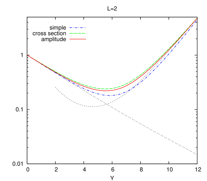
Figure 6: The gap cross section in the three matching schemes for $L=2$ ($\alpha_{s}=0.2$) compared to $\sigma_{BFKL}$ (dots) and $\sigma$ (double-dots)

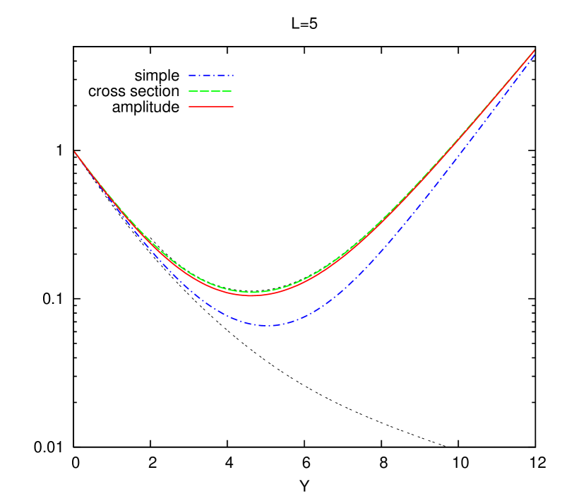
Figure 7: The gap cross section in the three matching schemes for $L=5$ ($\alpha_{s}=0.2$) compared to $\sigma_{BFKL}$ (dots) and $\sigma$ (double-dots)

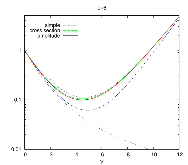
Figure 8: The gap cross section in the three matching schemes for $L=6$ ($\alpha_{s}=0.2$) compared to $\sigma_{BFKL}$ (dots) and $\sigma$ (double-dots)

We stress again that all three approaches are formally equally valid and equally phenomenological, in the sense that they cannot be justified by a finite order-by-order expansion. Only with a better understanding of the real-emission contributions in the high energy limit, which also have finite all-orders expressions but cancel these divergences order by order, can a more formally-justified matching be set up. We reserve this for future work.

4 Conclusion

Working in the high energy limit we have calculated the (partonic) cross section for the production of two jets distant in rapidity and with limited transverse energy flow into the region between the jets. Besides the DLL terms, we have summed terms sub-leading in $Y$ stemming from the imaginary parts of the loop integrals. This allowed us to identify those contributions that are also included in the fixed order $2\to 2$ BFKL cross section. We have shown that the leading order BFKL cross section, corresponding to the squared 1-loop amplitude, is entirely contained in the $\pi^{2}DLLA$. We derived an expression that consistently includes the terms of the $LLQ_{0}$ series and the BFKL series to $\mathcal{O}(\alpha_{s}^{5})$ accuracy without double counting. In the $LLQ_{0}A$, the inclusion of higher orders of the BFKL cross section in this way is not possible since it implies a divergent cross section.

We have also studied several phenomenological “all order” matching schemes that effectively interpolate between the $LLQ_{0}$ and BFKL results. Although they all yield similar results, the differences between them cannot be resolved without further work, specifically understanding the role of real-emission contributions in the high energy limit.

In this paper we have made a first step towards the unification of the two main approaches to the “jet–gap–jet” process. The question remains as to how they can be fully combined.

Appendix A Elastic Scattering Amplitudes in $d$ Dimensions

We calculate the elastic quark-quark amplitude in the high energy limit in the approximation of strongly-ordered transverse momenta of the $t$-channel gluons. We work in the eikonal effective theory. The transverse momentum of the softest gluon is taken to be larger than $Q_{0}$. Since we need the singlet exchange amplitude for $Q_{0}=0$ we consider $d=4-2\epsilon$ dimensions. We work in Feynman gauge. Denoting the color indices of the initial and final state quark pair by ${ik}$ and ${jl}$, respectively, the colour operators for singlet and octet exchange are

$$\mathbf{C}_{1}=\delta_{ij}\delta_{kl}\quad,\qquad\mathbf{C}_{8}=\frac{1}{2}(\delta_{il}\delta_{jk}-\frac{1}{N_{c}}\delta_{ij}\delta_{kl}).$$

The tree level amplitude reads:

$$\mathcal{A}^{(0)}\mathbf{C}_{8}=-g_{s}^{2}\mu^{2\epsilon}\frac{2\hat{s}}{Q^{2}}\mathbf{C}_{8}$$ (98)

A.1 The one loop amplitude

There are two Feynman diagrams, the box and the crossed box. In each of them there are two configurations of strong ordering possible giving the same result, so we collect them together:

$$\mathcal{A}_{\Box}\mathbf{C}_{\Box} =2\mathcal{A}^{(0)}\,\int\frac{d^{d}k}{(2\pi)^{d}}\bar{f}(k)\Theta(Q^{2}-\mathbf{k}^{2})\Theta(\mathbf{k}^{2}-Q_{0}^{2})\mathbf{C}_{\Box},$$ (99)

$$\bar{f}(k)=ig^{2}_{s}\mu^{2\epsilon}\;\frac{p_{1}\cdot p_{2}}{(p_{1}k-i\epsilon)(p_{2}k+i\epsilon)(k^{2}+i\epsilon)};$$ (100)

$$\mathcal{A}_{{\,\scalebox{0.67}{\rotatebox{90.0}{$\Join$}}}}\mathbf{C}_{{\,\scalebox{0.67}{\rotatebox{90.0}{$\Join$}}}} =2\mathcal{A}^{(0)}\,\int\frac{d^{d}k}{(2\pi)^{d}}f(k)\Theta(Q^{2}-\mathbf{k}^{2})\Theta(\mathbf{k}^{2}-Q_{0}^{2})\mathbf{C}_{{\,\scalebox{0.67}{\rotatebox{90.0}{$\Join$}}}},$$ (101)

$$f(k)=-ig^{2}_{s}\mu^{2\epsilon}\;\frac{p_{1}\cdot p_{2}}{(p_{1}k-i\epsilon)(p_{2}k-i\epsilon)(k^{2}+i\epsilon)}.$$ (102)

We have again extracted the colour factors explicitly, $\mathbf{C}_{\Box}$ and $\mathbf{C}_{\,\scalebox{0.67}{\rotatebox{90.0}{$\Join$}}}$. $\mathbf{k}$ is the usual transverse part of $k$ ($\mathbf{k}^{2}>0$). The upper limit on $\mathbf{k}^{2}$ as imposed by the $\Theta$ function is a consequence of the strong ordering condition. Simple colour algebra gives

$$\mathbf{C}_{\Box} = \;\;\,\phantom{\frac{N_{c}}{2}}-\frac{1}{N_{c}}\;\;\,\mathbf{C}_{8}+\frac{N_{c}^{2}-1}{4N_{c}^{2}}\mathbf{C}_{1},$$ (103)

$$\mathbf{C}_{\,\scalebox{0.67}{\rotatebox{90.0}{$\Join$}}} = \left(\frac{N_{c}}{2}-\frac{1}{N_{c}}\right)\mathbf{C}_{8}+\frac{N_{c}^{2}-1}{4N_{c}^{2}}\mathbf{C}_{1}.$$ (104)

Putting together the terms and performing some simplification, we arrive at

$$\mathcal{A}^{(1)}\mathbf{C} \equiv \mathcal{A}_{\Box}\mathbf{C}_{\Box}+i\mathcal{A}_{\,\scalebox{0.67}{\rotatebox{90.0}{$\Join$}}}\mathbf{C}_{\,\scalebox{0.67}{\rotatebox{90.0}{$\Join$}}}$$ (105)

$$= \mathcal{A}^{(0)}\left(\frac{N_{c}^{2}-1}{4N_{c}^{2}}\mathcal{G}\,\mathbf{C}_{1}+\left(\frac{N_{c}}{2}\mathcal{F}-\frac{1}{N_{c}}\mathcal{G}\right)\mathbf{C}_{8}\right),$$ (106)

with

$$\mathcal{F} = 2\int\frac{\mathrm{d}^{d}k}{(2\pi)^{d}}f(k)\;\Theta(Q^{2}-\mathbf{k}^{2})\Theta(\mathbf{k}^{2}-Q_{0}^{2}),$$ (107)

$$\mathcal{G} = 2\int\frac{\mathrm{d}^{d}k}{(2\pi)^{d}}[f(k)+\bar{f}(k)]\;\Theta(Q^{2}-\mathbf{k}^{2})\Theta(\mathbf{k}^{2}-Q_{0}^{2})$$ (108)

We introduce Sudakov variables and perform the integration with respect to two of them. The angular integration in the transverse momentum integral is trivial and as the result for $\mathcal{F}$ and $\mathcal{G}$ we obtain ($d=4-2\epsilon$):

$$\mathcal{F} =-\frac{2\alpha_{s}}{\pi}\;\frac{(4\pi\mu^{2})^{\epsilon}}{\Gamma(1-\epsilon)}\,Y\,\int^{Q}_{Q_{0}}\frac{\mathrm{d}k}{k^{1+2\epsilon}}$$ (109)

$$\mathcal{G} =-\frac{2\alpha_{s}}{\pi}\;\frac{(4\pi\mu^{2})^{\epsilon}}{\Gamma(1-\epsilon)}\,(i\pi)\,\int^{Q}_{Q_{0}}\frac{\mathrm{d}k}{k^{1+2\epsilon}}$$ (110)

Note that the real parts from $f$ and $\bar{f}$ in $\mathcal{G}$ (108) and hence the terms proportional to $Y$ have cancelled.

A.2 The two loop amplitude

Figure 9: The 2-loop amplitude

According to the colour structure there are four groups of Feynman diagrams (Fig.9). For each group there are four configurations of strong ordering giving the same result. In terms of the functions $f$ and $\bar{f}$, (102,100) the amplitudes read:

$$\mathcal{A}^{(2)}_{x}\mathbf{C}_{x} =4\mathcal{A}^{(0)}\int\frac{d^{d}k_{1}}{(2\pi)^{d}}\int\frac{d^{d}k_{2}}{(2\pi)^{d}}\;a_{x}(k_{1},k_{2})\;\Theta(Q^{2}-\mathbf{k}_{1}^{2})\Theta(\mathbf{k}_{1}^{2}-\mathbf{k}_{2}^{2})\Theta(\mathbf{k}_{2}^{2}-Q_{0}^{2})\;\mathbf{C}_{x}$$

$$x=a,b,c,d$$

with

$$a_{a}(k_{1},k_{2}) =\bar{f}(k_{1})\bar{f}(k_{2})$$ (111)

$$a_{b}(k_{1},k_{2}) =f(k_{1})\bar{f}(k_{2})$$ (112)

$$a_{c}(k_{1},k_{2}) =\bar{f}(k_{1})f(k_{2})$$ (113)

$$a_{d}(k_{1},k_{2}) =f(k_{1})f(k_{2})$$ (114)

We can express each amplitude in terms of $\mathcal{F}$ and $\mathcal{G}$ since the $\Theta$-functions only affect the integration over the absolute value of the transverse momentum which we left undone in $\mathcal{F}$ and $\mathcal{G}$, (109,110). The decomposition of the sum of the four amplitudes in terms of $\mathbf{C}_{8}$ and $\mathbf{C}_{1}$ is straightforward. We finally find for the two-loop amplitude ($\mathbf{C}$ being the corresponding colour factor):

$$\mbox{$\mathrm{I\!Re}$}(\mathcal{A}^{(2)}\mathbf{C}) =\mathcal{A}^{(0)}\frac{1}{2}\left[|\mathcal{G}|^{2}\frac{N_{c}^{2}-1}{4N_{c}^{3}}\mathbf{C}_{1}+\left(\frac{N_{c}^{2}}{4}\mathcal{F}^{2}-\frac{N_{c}^{2}+3}{4N_{c}^{2}}|\mathcal{G}|^{2}\right)\mathbf{C}_{8}\right]$$ (115)

$$\mbox{$\mathrm{I\!Im}$}(\mathcal{A}^{(2)}\mathbf{C}) =\mathcal{A}^{(0)}\frac{1}{2}|\mathcal{G}|\mathcal{F}\left[\frac{N_{c}^{2}-1}{8N_{c}}\mathbf{C}_{1}-\mathbf{C}_{8}\right].$$ (116)

Note that the sub-leading terms in the real part of $\mathcal{A}^{(2)}$ stem from keeping the sub-leading imaginary part of the one loop result.