UAB-FT 560

hep-ph/0502060

February 2005

Probing New Physics Via the Transverse Amplitudes of ${B}^{0}\to K^{*0}(\to K^{-}\pi^{+})l^{+}l^{-}$ at Large Recoil

Frank Krüger^1, and Joaquim Matias^2,
1Munich University of Applied Sciences, D-80335 München, Germany

²IFAE, Universitat Autònoma de Barcelona, 08193 Bellaterra, Barcelona, Spain

We perform an analysis of the $K^{*}$ polarization states in the exclusive $B$ meson decay ${B}^{0}\to~{}K^{*0}(\to K^{-}\pi^{+})l^{+}l^{-}$ ($l=e,\mu,\tau$) in the low dilepton mass region, where the final vector meson has a large energy. Working in the transversity basis, we study various observables that involve the $K^{*}$ spin amplitudes ${A}_{\bot}$, $A_{\|}$, $A_{0}$ by exploiting the heavy-to-light form factor relations in the heavy quark and large-$E_{K^{*}}$ limit. We find that at leading order in $1/m_{b}$ and $\alpha_{s}$ the form-factor dependence of the asymmetries that involve transversely polarized $K^{*}$ completely drops out. At next-to-leading logarithmic order, including factorizable and non-factorizable corrections, the theoretical errors for the transverse asymmetries turn out to be small in the standard model (SM). Integrating over the lower part of the dimuon mass region, and varying the theoretical input parameters, the SM predicts ${\mathcal{A}}_{T}^{(1)}=0.9986\pm 0.0002$ and ${\mathcal{A}}_{T}^{(2)}=-0.043\pm 0.003$. In addition, the longitudinal and transverse polarization fractions are found to be $(69\pm 3)\%$ and $(31\pm 3)\%$ respectively, so that $\Gamma_{L}/\Gamma_{T}=2.23\pm 0.31$. Beyond the SM, we focus on new physics that mainly gives sizable contributions to the coefficients $C_{7}^{\mathrm{eff}(\prime)}$ of the electromagnetic dipole operators. Taking into account experimental data on rare $B$ decays, we find large effects of new physics in the transverse asymmetries. Furthermore, we show that a measurement of longitudinal and transverse polarization fractions will provide complementary information on physics beyond the SM.

PACS number(s): 13.20.He, 13.25.Hw

1 Introduction

The decay ${B^{0}}\to K^{*0}(\to K^{-}\pi^{+})l^{+}l^{-}$, where $l$ stands for $e,\mu,\tau$, is interesting as a testing ground for the standard model (SM) and its extensions [1, 2, 3, 4, 5, 6, 7, 8, 9]. In particular, it has been shown that a study of the angular distribution of the four-body final state allows to search for right-handed currents [1, 3] and provides additional information on CP violation [2].

Since the exclusive $B^{0}\to K^{*0}l^{+}l^{-}$ decay involves the heavy-to-light transition form factors parametrizing the hadronic matrix elements, it usually suffers from large theoretical uncertainties, which amount to $\sim 30\%$ on the branching ratio [8, 9]. However, the theoretical errors can be reduced by exploiting relations between the form factors that emerge in the limit where the initial hadron is heavy and the final meson has a large energy [10]. In this case, the seven a priori independent $B\to K^{*}$ transition form factors can be expressed through merely two universal form factors at leading power in $1/m_{b}$ and $\alpha_{s}$ [10]. While this reduces the hadronic uncertainties in the calculation of exclusive $B$ decays, it restricts the validity of the theoretical predictions to the dilepton mass region below the $J/\psi$ mass. Corrections to the heavy quark and large energy limit, at next-to-leading logarithmic (NLL) order, have been computed in [11, 12] including factorizable and non-factorizable contributions. (The corrections to the heavy-to-light form factors at large recoil energy can be calculated systematically within the soft-collinear effective theory [13].)

In this paper, we study various observables that involve different combinations of $K^{*}$ spin amplitudes, whose moduli and phases can be extracted from an analysis of the angular distribution of ${B}^{0}\to K^{*0}(\to K^{-}\pi^{+})l^{+}l^{-}$ [2]. In order to reduce the uncertainties due to the hadronic form factors, we concentrate on quantities that contain only ratios of $K^{*}$ polarization amplitudes. Special emphasis is put on those observables that involve transversely polarized $K^{*}$, which turn out to be largely independent of the hadronic form factors, even after including NLL corrections. We also make use of the NLL order corrections [11, 12], as a first approach, to study the robustness of the set of observables analysed below. Subleading effects in the heavy quark expansion [7, 14] will be included elsewhere.

Our paper is organized as follows. In Sec. 2 we setup our theoretical framework. Section 3 contains the angular distribution in the transversity basis and the polarization amplitudes of the final vector meson. In Sec. 4 we discuss various observables that are sensitive to the polarization states of $K^{*}$. We study in detail the implications of factorizable and non-factorizable corrections to these observables in the SM. The impact of new physics is investigated in a model-independent manner. In particular, the implications of right-handed currents in the low dilepton invariant mass region are examined. Our summary and conclusions can be found in Sec. 5. For the paper to be self-contained, we provide in the appendix the angular distribution of ${B}^{0}\to K^{*0}(\to K^{-}\pi^{+})l^{+}l^{-}$ including lepton-mass effects.

2 Theoretical framework

We begin with the matrix element of the decay ${B^{0}}\to K^{*0}(\to K^{-}\pi^{+})l^{+}l^{-}$, which may be obtained by using the effective Hamiltonian describing the $b\to sl^{+}l^{-}$ transition [1, 2, 3]. It can be written as [15]

$${\mathcal{H}}_{\mathrm{eff}}=-\frac{4G_{F}}{\sqrt{2}}V_{tb}V_{ts}^{*}\sum_{i=1}^{10}[C_{i}(\mu){\mathcal{O}}_{i}(\mu)+C_{i}^{\prime}(\mu){\mathcal{O}}_{i}^{\prime}(\mu)],$$ (2.1)

where $C_{i}^{(\prime)}(\mu)$ and ${\mathcal{O}}_{i}^{(\prime)}(\mu)$ are the Wilson coefficients and local operators respectively. For a complete set of operators in the SM (i.e. ${\mathcal{O}}_{i}$’s) and beyond, we refer to [15, 16, 17].

In our subsequent analysis, we concentrate on

$${\mathcal{O}}_{7}=\frac{e}{16\pi^{2}}m_{b}(\bar{s}\sigma_{\mu\nu}P_{R}b)F^{\mu\nu},\quad{\mathcal{O}}_{9}=\frac{e^{2}}{16\pi^{2}}(\bar{s}\gamma_{\mu}P_{L}b)(\bar{l}\gamma^{\mu}l),\quad{\mathcal{O}}_{10}=\frac{e^{2}}{16\pi^{2}}(\bar{s}\gamma_{\mu}P_{L}b)(\bar{l}\gamma^{\mu}\gamma_{5}l),$$

where $P_{L,R}=(1\mp\gamma_{5})/2$ and $m_{b}\equiv m_{b}(\mu)$ is the running mass in the $\overline{\mbox{MS}}$ scheme. As for the primed operators [16, 17], we restrict ourselves to

$${\mathcal{O}}_{7}^{\prime}=\frac{e}{16\pi^{2}}m_{b}(\bar{s}\sigma_{\mu\nu}P_{L}b)F^{\mu\nu}.$$ (2.3)

(Below we show how to include the chiral partners of ${\cal O}_{9,10}$ in our analysis.) Since there are no right-handed currents in the SM, the coefficient accompanying ${\mathcal{O}}_{7}^{\prime}$ is non-zero only in certain extensions of the SM such as the left-right model [16] and the unconstrained supersymmetric standard model [17].

2.1 Matrix element

Given the above Hamiltonian, the matrix element can be written as

$${\mathcal{M}} = \frac{G_{F}\alpha}{\sqrt{2}\pi}V_{tb}V_{ts}^{*}\bigg{\{}\bigg{[}C_{9}^{\text{eff}}\langle K\pi|(\bar{s}\gamma^{\mu}P_{L}b)|B\rangle-\frac{2m_{b}}{q^{2}}\langle K\pi|\bar{s}i\sigma^{\mu\nu}q_{\nu}(C_{7}^{\text{eff}}P_{R}+{C_{7}^{\text{eff}}}^{\prime}P_{L})b|B\rangle\bigg{]}(\bar{l}\gamma_{\mu}l)$$ (2.4)

$$+ C_{10}\langle K\pi|(\bar{s}\gamma^{\mu}P_{L}b)|B\rangle(\bar{l}\gamma_{\mu}\gamma_{5}l)\bigg{\}},$$

where $q$ is the four-momentum of the lepton pair. Explicit expressions for the short-distance coefficients, including next-to-next-to-leading logarithmic (NNLL) corrections, can be found in Refs. [18, 19, 20].

The hadronic part of the matrix element describing the $B\to K\pi$ transition can be parametrized in terms of $B\to K^{*}$ form factors by means of a narrow-width approximation [2]. The relevant form factors are defined as [21, 8]:

$$\langle{K^{*}}(p_{{K^{*}}})|\bar{s}\gamma_{\mu}P_{L,R}b|{B}(p)\rangle=i\epsilon_{\mu\nu\alpha\beta}\epsilon^{\nu*}p^{\alpha}q^{\beta}\frac{V(s)}{m_{B}+m_{{K^{*}}}}\mp\frac{1}{2}\bigg{\{}\epsilon_{\mu}^{*}(m_{B}+m_{{K^{*}}})A_{1}(s)$$ (2.5)

$$- (\epsilon^{*}\cdot q)(2p-q)_{\mu}\frac{A_{2}(s)}{m_{B}+m_{{K^{*}}}}-\frac{2m_{{K^{*}}}}{s}(\epsilon^{*}\cdot q)[A_{3}(s)-A_{0}(s)]q_{\mu}\bigg{\}},$$

where

$$A_{3}(s)=\frac{m_{B}+m_{{K^{*}}}}{2m_{{K^{*}}}}A_{1}(s)-\frac{m_{B}-m_{{K^{*}}}}{2m_{{K^{*}}}}A_{2}(s),$$ (2.6)

and

$$\langle{K^{*}}(p_{{K^{*}}})|\bar{s}i\sigma_{\mu\nu}q^{\nu}P_{R,L}b|{B}(p)\rangle=-i\epsilon_{\mu\nu\alpha\beta}\epsilon^{\nu*}p^{\alpha}q^{\beta}T_{1}(s)\pm\frac{1}{2}\bigg{\{}[\epsilon_{\mu}^{*}(m_{B}^{2}-m_{{K^{*}}}^{2})$$ (2.7)

$$- (\epsilon^{*}\cdot q)(2p-q)_{\mu}]T_{2}(s)+(\epsilon^{*}\cdot q)\bigg{[}q_{\mu}-\frac{s}{m_{B}^{2}-m_{{K^{*}}}^{2}}(2p-q)_{\mu}\bigg{]}T_{3}(s)\bigg{\}}.$$

In the above, $q=p_{l^{+}}+p_{l^{-}}$, $s=q^{2}$, and $\epsilon^{\mu}$ is the $K^{*}$ polarization vector.

2.2 Heavy-to-light form factors at large recoil

As we have already mentioned, interesting relations between the hadronic form factors emerge in the limit where the initial hadron is heavy and the final meson has a large energy [10]. In this case, the form factors can be expanded in the small ratios $\Lambda_{\mathrm{QCD}}/m_{b}$ and $\Lambda_{\mathrm{QCD}}/E$, where $E$ is the energy of the light meson. Neglecting corrections of order $1/m_{b}$ and $\alpha_{s}$, the seven a priori independent $B\to K^{*}$ form factors in Eqs. (2.5) and (2.7) reduce to two universal form factors $\xi_{\bot}$ and $\xi_{\|}$ [10, 11]:

$$A_{1}(s)=\frac{2E_{K^{*}}}{m_{B}+m_{K^{*}}}\xi_{\bot}(E_{K^{*}}),$$ (2.8a)

$$A_{2}(s)=\frac{m_{B}}{m_{B}-m_{K^{*}}}\bigg{[}\xi_{\bot}(E_{K^{*}})-\xi_{\|}(E_{K^{*}})\bigg{]},$$ (2.8b)

$$A_{0}(s)=\frac{E_{K^{*}}}{m_{K^{*}}}\xi_{\|}(E_{K^{*}}),$$ (2.8c)

$$V(s)=\frac{m_{B}+m_{K^{*}}}{m_{B}}\xi_{\bot}(E_{K^{*}}),$$ (2.8d)

$$T_{1}(s)=\xi_{\bot}(E_{K^{*}}),$$ (2.8e)

$$T_{2}(s)=\frac{2E_{K^{*}}}{m_{B}}\xi_{\bot}(E_{K^{*}}),$$ (2.8f)

$$T_{3}(s)=\xi_{\bot}(E_{K^{*}})-\xi_{\|}(E_{K^{*}}).$$ (2.8g)

Here, $E_{K^{*}}$ is the energy of the final vector meson in the ${B}$ rest frame,

$$E_{K^{*}}\simeq\frac{m_{B}}{2}\left(1-\frac{s}{m_{B}^{2}}\right).$$ (2.9)

Since the theoretical predictions are restricted to the kinematic region in which the energy of the $K^{*}$ is of the order of the heavy quark mass (i.e. $s\ll m_{B}^{2}$), we confine our analysis to the dilepton mass in the range $2m_{l}\leqslant M_{l^{+}l^{-}}\leqslant 2.5\ {\text{GeV}}$. The relations in Eqs. (2.8) are valid for the soft contribution to the form factors at large recoil, and are violated by symmetry breaking corrections of order $\alpha_{s}$ and $1/m_{b}$. The corrections at first order in $\alpha_{s}$ have been computed in [11, 12] and will be discussed in more detail in Sec. 4.2. However, it should be noted that the ratios $A_{1}/V$ and $T_{1}/T_{2}$ do not receive $\alpha_{s}$ corrections to leading power in $1/E_{K^{*}}$ [11, 22]. This in turn leads to a specific behaviour of the amplitudes describing the transverse polarization states of the $K^{*}$ in the heavy quark and large energy limit, as explained below.

3 Angular distribution and transversity amplitudes

Assuming the $K^{*}$ to be on the mass shell, the decay ${B^{0}}\to K^{*0}(\to K^{-}\pi^{+})l^{+}l^{-}$ is completely described by four independent kinematic variables; namely, the lepton-pair invariant mass, $s$, and the three angles $\theta_{l}$, $\theta_{K^{*}}$, $\phi$. In terms of these variables, the differential decay rate can be written as [2]

$$\frac{d^{4}\Gamma}{ds\,d\cos\theta_{l}\,d\cos\theta_{K^{*}}\,d\phi}=\frac{9}{32\pi}\sum_{i=1}^{9}I_{i}(s,\theta_{K^{*}})f_{i}(\theta_{l},\phi),$$ (3.1)

where $I_{i}$ depend on products of the four $K^{*}$ spin amplitudes ${A}_{\bot}$, $A_{\|}$, $A_{0}$, $A_{t}$, and $f_{i}$ are the corresponding angular distribution functions (see Appendix A for details). Note that $A_{t}$ is related to the time-like component of the virtual $K^{*}$, which does not contribute in the case of massless leptons.

Given the matrix element in Eq. (2.4), we obtain for the transversity amplitudes

$$A_{\bot L,R}=N\sqrt{2}\lambda^{1/2}\bigg{[}(C_{9}^{\text{eff}}\mp C_{10})\frac{V(s)}{m_{B}+m_{K^{*}}}+\frac{2m_{b}}{s}(C_{7}^{\text{eff}}+{C_{7}^{\text{eff}}}^{\prime})T_{1}(s)\bigg{]},$$ (3.2)

$$A_{\|L,R}=-N\sqrt{2}(m_{B}^{2}-m_{K^{*}}^{2})\bigg{[}(C_{9}^{\text{eff}}\mp C_{10})\frac{A_{1}(s)}{m_{B}-m_{K^{*}}}+\frac{2m_{b}}{s}(C_{7}^{\text{eff}}-{C_{7}^{\text{eff}}}^{\prime})T_{2}(s)\bigg{]},$$ (3.3)

$$A_{0L,R} = -\frac{N}{2m_{K^{*}}\sqrt{s}}\bigg{[}(C_{9}^{\text{eff}}\mp C_{10})\bigg{\{}(m_{B}^{2}-m_{K^{*}}^{2}-s)(m_{B}+m_{K^{*}})A_{1}(s)-\lambda\frac{A_{2}(s)}{m_{B}+m_{K^{*}}}\bigg{\}}$$ (3.4)

$$+ {2m_{b}}(C_{7}^{\text{eff}}-{C_{7}^{\text{eff}}}^{\prime})\bigg{\{}(m_{B}^{2}+3m_{K^{*}}^{2}-s)T_{2}(s)-\frac{\lambda}{m_{B}^{2}-m_{K^{*}}^{2}}T_{3}(s)\bigg{\}}\bigg{]},$$

$$A_{t}=\frac{2N}{\sqrt{s}}\lambda^{1/2}C_{10}A_{0}(s),$$ (3.5)

which are related to the helicity amplitudes used, e.g., in [1, 3, 6] through

$$A_{\bot,\|}=(H_{+1}\mp H_{-1})/\sqrt{2},\quad A_{0}=H_{0},\quad A_{t}=H_{t}.$$ (3.6)

In the above formulae, $\lambda=m_{B}^{4}+m_{K^{*}}^{4}+s^{2}-2(m_{B}^{2}m_{K^{*}}^{2}+m_{K^{*}}^{2}s+m_{B}^{2}s)$ and

$$N=\left[\frac{G_{F}^{2}\alpha^{2}}{3\cdot 2^{10}\pi^{5}m_{B}^{3}}|V_{tb}V_{ts}^{\ast}|^{2}s\lambda^{1/2}\left(1-\frac{4m_{l}^{2}}{s}\right)^{1/2}\right]^{1/2}.$$ (3.7)

Note that the contributions of the chirality-flipped operators ${\mathcal{O}}_{9,10}^{\prime}={\mathcal{O}}_{9,10}(P_{L}\to P_{R})$ can be included in the above amplitudes by the replacements $C^{(\mathrm{eff})}_{9,10}\to C^{(\mathrm{eff})}_{9,10}+C^{(\mathrm{eff})\prime}_{9,10}$ in Eq. (3.2), $C_{9,10}^{(\mathrm{eff})}\to C^{(\mathrm{eff})}_{9,10}-C^{(\mathrm{eff})\prime}_{9,10}$ in Eqs. (3.3) and (3.4), and $C_{10}\to C_{10}-C_{10}^{\prime}$ in Eq. (3.5).

3.1 Transversity amplitudes at large recoil

The transversity amplitudes in Eqs. (3.2)–(3.5) take a particularly simple form in the heavy quark and large energy limit. In fact, exploiting the form factor relations in Eqs. (2.8), we obtain at leading order in $1/m_{b}$ and $\alpha_{s}$

$$A_{\bot L,R}=\sqrt{2}Nm_{B}(1-\hat{s})\bigg{[}(C_{9}^{\text{eff}}\mp C_{10})+\frac{2\hat{m}_{b}}{\hat{s}}(C_{7}^{\text{eff}}+{C_{7}^{\text{eff}}}^{\prime})\bigg{]}\xi_{\bot}(E_{K^{*}}),$$ (3.8)

$$A_{\|L,R}=-\sqrt{2}Nm_{B}(1-\hat{s})\bigg{[}(C_{9}^{\text{eff}}\mp C_{10})+\frac{2\hat{m}_{b}}{\hat{s}}(C_{7}^{\text{eff}}-{C_{7}^{\text{eff}}}^{\prime})\bigg{]}\xi_{\bot}(E_{K^{*}}),$$ (3.9)

$$A_{0L,R}=-\frac{Nm_{B}}{2\hat{m}_{K^{*}}\sqrt{\hat{s}}}(1-\hat{s})^{2}\bigg{[}(C_{9}^{\text{eff}}\mp C_{10})+2\hat{m}_{b}(C_{7}^{\text{eff}}-{C_{7}^{\text{eff}}}^{\prime})\bigg{]}\xi_{\|}(E_{K^{*}}),$$ (3.10)

$$A_{t}=\frac{Nm_{B}}{\hat{m}_{K^{*}}\sqrt{\hat{s}}}(1-\hat{s})^{2}C_{10}\xi_{\|}(E_{K^{*}}),$$ (3.11)

with $\hat{s}=s/m_{B}^{2}$, $\hat{m}_{i}=m_{i}/m_{B}$. In writing Eqs. (3.8)–(3.11) we have dropped terms of $O(\hat{m}_{K^{*}}^{2})$. From inspection of these formulae, we infer the following features.

(i) Within the SM, we recover the naive quark-model prediction of $A_{\bot}=-A_{\|}$ [23, 24] in the $m_{B}\to\infty$ and $E_{K^{*}}\to\infty$ limit (equivalently $\hat{m}_{K^{*}}^{2}\to 0$). In this case, the $s$ quark is produced in helicity $-{1}/{2}$ by weak interactions in the limit $m_{s}\to 0$, which is not affected by strong interactions in the massless case [22]. Thus, the strange quark combines with a light quark to form a $K^{*}$ with helicity either $-1$ or $0$ but not $+1$. Consequently, the SM predicts at quark level $H_{+1}=0$, and hence $A_{\bot}=-A_{\|}$ [cf. Eq. (3.6)], which is revealed as $|H_{-1}|\gg|H_{+1}|$ (or $A_{\bot}\approx-A_{\|}$) at the hadron level.

(ii) The longitudinal and time-like (transverse) polarizations of the $K^{*}$ involve only the universal form factors $\xi_{\|}$ ($\xi_{\bot}$) in the $m_{B}\to\infty$ and $E_{K^{*}}\to\infty$ limit.

4 $K^{*}$ polarization as a probe of new physics

4.1 Observables

The study of the angular distribution in the decay ${B^{0}}\to K^{*0}(\to K^{-}\pi^{+})l^{+}l^{-}$ allows a determination of the $K^{*}$ spin amplitudes along with their relative phases (see Appendix A). In order to minimize the theoretical uncertainties due to the hadronic form factors, we consider only those observables that involve ratios of amplitudes. (For a discussion of the error on the decay amplitudes of $B^{0}\to K^{*0}l^{+}l^{-}$, we refer to Ref. [6].)

Introducing the shorthand notation

$$A_{i}A^{*}_{j}\equiv A_{iL}(s)A^{*}_{jL}(s)+A_{iR}(s)A^{*}_{jR}(s)\quad(i,j=0,\|,\perp),$$ (4.1)

we investigate the following observables.

(i) Transverse asymmetries

$$A^{(1)}_{{T}}({s})=\frac{-2{\text{Re}}(A_{\|}{A}_{\bot}^{*})}{|{A}_{\bot}|^{2}+|A_{\|}|^{2}},\quad A^{(2)}_{{T}}({s})=\frac{|{A}_{\bot}|^{2}-|A_{\|}|^{2}}{|{A}_{\bot}|^{2}+|A_{\|}|^{2}}.$$ (4.2)

(ii) $K^{*}$ polarization parameter

$$\alpha_{K^{*}}(s)=\frac{2|{A}_{0}|^{2}}{|{A}_{\|}|^{2}+|{A}_{\perp}|^{2}}-1.$$ (4.3)

For final states with $l=e$ or $\mu$ it can be directly determined from the two-dimensional differential decay rate $d\Gamma/(ds\,d\cos\theta_{K^{*}})\propto[1+\alpha_{K^{*}}(s)\cos^{2}\theta_{K^{*}}]$, since the corresponding lepton-mass corrections are negligibly small.

(iii) Fraction of $K^{*}$ polarization

$$F_{L}(s)=\frac{|{A}_{0}|^{2}}{|{A}_{0}|^{2}+|{A}_{\|}|^{2}+|A_{\perp}|^{2}},\quad F_{T}(s)=\frac{|{A}_{\bot}|^{2}+|{A}_{\|}|^{2}}{|{A}_{0}|^{2}+|{A}_{\|}|^{2}+|A_{\perp}|^{2}},$$ (4.4)

so that $\alpha_{K^{*}}=2F_{L}/F_{T}-1$.

(iv) Integrated quantities ${\mathcal{A}}^{(1)}_{{T}}$, ${\mathcal{A}}^{(2)}_{{T}}$, $\mbox{\boldmath$\alpha$}_{K^{*}}$, and ${\mathcal{F}}_{L,T}$, which are obtained from the ones above by integrating numerator and denominator separately over the dilepton invariant mass.

4.2 SM prediction for the $K^{*}$ polarization

In this section we perform a detailed analysis of the previously defined observables within the SM. Following the work of Beneke et al. [12], we include factorizable and non-factorizable corrections at NLL order. Since these results are applicable only to the region where $s\lesssim 4m_{c}^{2}$, we consider in the remainder of this paper muons in the final state with $2m_{\mu}\leqslant M_{\mu^{+}\mu^{-}}\leqslant 2.5\ {\text{GeV}}$.

To include the NLL corrections to the transversity amplitudes in the SM, we set ${C_{7}^{\text{eff}}}^{\prime}=0$ in Eqs. (3.2)–(3.4) and replace

$$C_{7}^{\text{eff}}T_{i}\rightarrow{\cal T}_{i},\quad C_{9}^{\text{eff}}\rightarrow C_{9}\quad(i=1,2,3),$$ (4.5)

with the Wilson coefficients $C_{9,10}$ taken at NNLL order (in the terminology of Ref. [12]). The ${\cal T}_{i}$ in Eq. (4.5) are given by

$${\cal T}_{1}={\cal T}_{\perp},\quad{\cal T}_{2}=\frac{2E_{{K^{*}}}}{m_{B}}{\cal T}_{\perp},\quad{\cal T}_{3}={\cal T}_{\perp}+{\cal T}_{\parallel},$$ (4.6)

where ${\cal T}_{a}$ ($a=\bot,\|$) contain factorizable (f) and non-factorizable (nf) contributions [12]:

$${\cal T}_{\perp} = \xi_{\perp}(0)\Bigg{\{}C_{\perp}^{(0)}\frac{1}{(1-s/m_{B}^{2})^{2}}+\frac{\alpha_{s}}{3\pi}\Bigg{[}\frac{C_{\perp}^{(1)}}{(1-s/m_{B}^{2})^{2}}+\kappa_{\perp}\lambda^{-1}_{B,+}\int_{0}^{1}du\,\Phi_{K^{*},\perp}(u)$$ (4.7)

$$\times [T_{\perp,+}^{(\mathrm{f})}(u)+T_{\perp,+}^{(\mathrm{nf})}(u)]\Bigg{]}\Bigg{\}},$$

$${\cal T}_{\parallel} = \xi_{\parallel}(0)\Bigg{\{}C_{\parallel}^{(0)}\frac{1}{{(1-s/m_{B}^{2})^{3}}}+\kappa_{\|}\frac{m_{K^{*}}}{E_{{K^{*}}}}\lambda^{-1}_{B,-}(s)\int_{0}^{1}du\,\Phi_{K^{*},\parallel}(u)\hat{T}_{\parallel,-}^{(0)}(u)$$ (4.8)

$$+ \frac{\alpha_{s}}{3\pi}\Bigg{[}\frac{C_{\parallel}^{(1)}}{(1-s/m_{B}^{2})^{3}}+\kappa_{\|}\frac{m_{K^{*}}}{E_{{K^{*}}}}\Bigg{(}\lambda^{-1}_{B,+}\int_{0}^{1}du\,\Phi_{K^{*},\parallel}(u)[T_{\parallel,+}^{(\mathrm{f})}(u)+T_{\parallel,+}^{(\mathrm{nf})}(u)]+\lambda^{-1}_{B,-}(s)$$

$$\times \int_{0}^{1}du\,\Phi_{K^{*},\parallel}(u)\hat{T}_{\parallel,-}^{(\mathrm{nf})}(u)\Bigg{)}\Bigg{]}\Bigg{\}},$$

with

$$\kappa_{a}=\frac{\pi^{2}f_{B}f_{K^{*},a}}{3m_{B}\xi_{a}(0)},\quad\hat{T}_{\parallel,\,-}^{(0,\mathrm{nf})}(u)=\frac{(m_{B}\omega-s-i\epsilon)}{m_{B}\omega}{T}_{\parallel,\,-}^{(0,\mathrm{nf})}(u,\omega).$$ (4.9)

Explicit expressions for the $T$’s, ${C}$’s, $\lambda^{-1}_{B,-}(s)$ and the light-cone wave functions $\Phi_{K^{*}a}$, together with the remaining input parameters, can be found in Ref. [12].

Let us now analyse the impact of the NLL corrections on the observables introduced in the preceding subsection. In particular, we are interested in the sensitivity of these quantities to a variation of the theoretical input parameters, which we take from Table $2$ of [12].

We proceed by computing the quantities defined in Eqs. (4.2)–(4.4) to NLL accuracy by replacing the Wilson coefficients according to Eq. (4.5). We find that the dependence on the actual values of the soft form factors $\xi_{\bot,\|}(0)$ plays an important role in certain observables, as can be seen from Eqs. (4.7) and (4.8). Furthermore, we have explored the sensitivity of the NLL result to the scale dependence of the observables, which is mainly due to the hard-scattering correction, by changing the scale $\mu$ from $m_{b}/2$ to $2m_{b}$. This scale dependence is, apart from the error on the soft form factors at $s=0$, the main source of uncertainty. We have included the errors associated with the input parameters in quadrature. Concerning a variation of $m_{c}/m_{b}$, which affects mainly the contributions to the matrix element of the chromomagnetic operator (specifically the functions $F^{(7,9)}_{1,2}$ in [19]), we have chosen the range $0.27\leqslant m_{c}/m_{b}\leqslant 0.31$ [19], together with the 3-loop running for the strong coupling constant.

Our results are summarized in Figs. 1 and 2. As expected, the transverse asymmetries $A^{(1)}_{T}({s})$ and $A^{(2)}_{T}({s})$ are the most promising observables. Indeed, from Eqs. (3.8)–(3.10) it is clear that the dependence on the hadronic form factors drops out in the asymmetries at leading order in $1/m_{b}$ and $\alpha_{s}$. In this case, neglecting terms of $O(m_{K^{*}}^{2}/m_{B}^{2})$, the SM predicts $A^{(1)}_{T}({s})\sim 1$ and $A^{(2)}_{T}({s})\sim 0$. At NLL order, the impact of the soft form factors depends on the relative size of the NLL corrections compared to the leading order ones. In Fig. 1, we plot $A^{(1,2)}_{T}$ versus the dimuon mass $M_{\mu^{+}\mu^{-}}$ including NLL order corrections [11, 12] to the form factor relations in Eqs. (2.8).

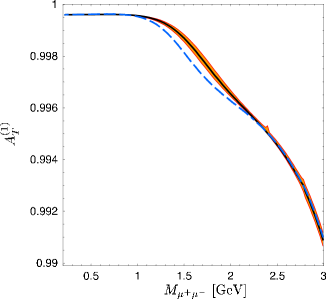
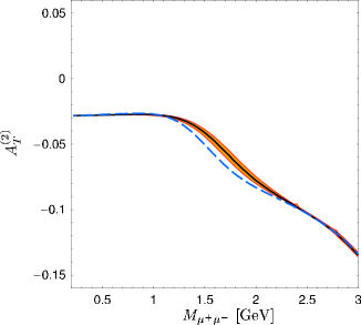
Figure 1: SM predictions for the asymmetries $A_{T}^{(1)}$ and $A_{T}^{(2)}$ as a function of the dimuon mass at LL (dashed line) and NLL (solid line). The shaded area has been obtained by varying the renormalization scale, the $b$-quark mass, $m_{c}/m_{b}$, the input parameters according to Ref. [12], and $\xi_{\perp}(0)$ as described in the text.

Note that the small cusp, e.g., in the left plot of Fig. 1 is due to a variation of $m_{c}$ and it is an artifact of the $c{\bar{c}}$ threshold in the charm loop diagrams. It is remarkable that there is only a small difference between the NLL result (solid curve) and the LL one (dashed curve). Furthermore, the sensitivity of the transverse asymmetries to the theoretical input parameters is rather weak. Indeed, neither the scale dependence nor the inclusion of the hadronic uncertainties (added in quadrature) induces large deviations. We stress that the shaded areas in Fig. 1 also take into account the possibility of a much smaller value for the soft form factor, namely $\xi_{\perp}(0)=0.24$, which is favoured by a fit to experimental data on ${\mathcal{B}}(B\rightarrow K^{*}\gamma)$ [12, 26]. The small impact of the theoretical uncertainties found, including the NLL corrections, shows the robustness of the transverse asymmetries and makes them an ideal place to search for new physics.

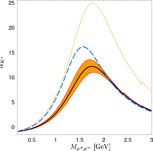
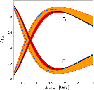
Figure 2: Left plot: The polarization parameter $\alpha_{K^{*}}$ at LL (dashed curve) and NLL (lower solid curve), as a function of the dimuon mass. The shaded area has been obtained by varying the theoretical input parameters for fixed $\xi_{\perp}(0)=0.35$ (see the text for details). To show the strong impact of $\xi_{\perp}(0)$, we also display the NLL result for $\xi_{\perp}(0)=0.24$ (upper solid curve). Right plot: The SM prediction for the $K^{*}$ polarization fractions, adopting the same conventions as before and allowing for a variation of $\xi_{\perp}(0)$ between $0.24$ and $0.35$. The inner dark region has been obtained by varying the theoretical input parameters for fixed $\xi_{\perp}(0)=0.35$.

The predictions for $\alpha_{K^{*}}$ and $F_{L,T}$ in the SM are shown in Fig. 2. As can be seen from the left plot in Fig. 2, there is a strong impact of the NLL corrections (solid curves) on $\alpha_{K^{*}}$. Moreover, the error band is substantially larger even for a fixed value of $\xi_{\perp}(0)=0.35$. A more detailed analysis of the dependence on the value of $\xi_{\perp}(0)$ shows that if we consider instead $\xi_{\perp}(0)=0.24$, which corresponds to the upper solid curve, the deviation would induce an even larger error band. In fact, as can be seen from the LL expressions in Eqs. (3.8)–(3.10), together with (4.3) and (4.4), there is no cancellation between the soft form factors. As a result, changing $\xi_{\perp}(0)$ from $0.35$ to $0.24$ should enhance the maximum of $\alpha_{K^{*}}$, as a function of the dimuon mass, by roughly a factor of two. This is also the case at NLL order, as can be inferred from the left plot in Fig. 2. The strong sensitivity of $\alpha_{K^{*}}$ to the poorly known quantity $\xi_{\perp}(0)$ therefore requires a better theoretical control on the soft form factor.

As far as $F_{L,T}$ are concerned, they also depend on $\xi_{\perp}(0)$, but the fact that the normalization factor includes $A_{0}$ reduces the impact on the soft form factor. The right plot in Fig. 2 shows the LL result (dashed curve), the NLL (solid curve) and two bands. The internal one includes all errors for fixed $\xi_{\perp}(0)=0.35$, while the wider band includes a variation of $\xi_{\perp}(0)$ between $0.24$ and $0.35$. Note that our results for the $K^{*}$ polarization fractions are slightly different from those of Ref. [6]. This can be traced to the different parametrization and normalization of the soft form factors appearing in Eqs. (3.8)–(3.11) (see Fig. 1 in [6]).

Finally, we have computed the integrated observables including NLL corrections and using $\xi_{\perp}(0)=0.35\pm 0.07$. Our results for the low dimuon mass region are listed in Table 1. Notice that the theoretical uncertainties of the asymmetries ${\mathcal{A}}_{T}^{(1,2)}$ amount to less then $7\%$, so that its measurement will allow a precise test of the SM.

Table 1: SM predictions for the observables defined in Eqs. (4.2)–(4.4) when integrated over the low dimuon mass region $2m_{\mu}\leqslant M_{\mu^{+}\mu^{-}}\leqslant 2.5\ {\text{GeV}}$. The form factors $\xi_{\bot,\|}$ and the input parameters are taken from Ref. [12].

${\mathcal{A}}_{T}^{(1)}$	${\mathcal{A}}_{T}^{(2)}$	$\mbox{\boldmath$\alpha$}_{K^{*}}$	${\mathcal{F}}_{L}$	${\mathcal{F}}_{T}$
$0.9986\pm 0.0002$	$-0.043\pm 0.003$	$3.47\pm 0.71$	$0.69\pm 0.03$	$0.31\pm 0.03$

4.3 Impact of new physics on the $K^{*}$ polarization

We now study model-independently the implications of right-handed currents for the observables defined in Eqs. (4.2)–(4.4). Since the low dimuon mass region is dominated by the photon pole, $|C_{7}^{\mathrm{eff}(\prime)}|^{2}/s$, we do not take into account the contributions of the chirality-flipped operators ${\cal O}_{9,10}^{\prime}$, but will allow for deviations of $C_{9,10}$ from their SM values. Examples of new-physics scenarios that could give sizable contributions to ${C_{7}^{\mathrm{eff}}}^{(\prime)}$ include the left-right model [16], the unconstrained minimal supersymmetric standard [17], and an $\mathrm{SO}(10)$ SUSY GUT model with large mixing between $\tilde{s}_{R}$ and $\tilde{b}_{R}$ [25].

In our analysis we use the Wilson coefficients and soft form factors $\xi_{\bot,\|}$ of Ref. [12]. Furthermore, we take, for simplicity, the leading-order condition

$$|{C_{7}^{\mathrm{eff}}}|^{2}+|{C_{7}^{\mathrm{eff}}}^{\prime}|^{2}\leqslant 1.2|{C_{7}^{\mathrm{eff},\mathrm{SM}}}|^{2},$$ (4.10)

which follows from the requirement that the theoretical prediction for ${\mathcal{B}}(B\to X_{s}\gamma)$ [27] is within $2\sigma$ of the experimental average $(3.52^{+0.30}_{-0.28})\times 10^{-4}$ [28]. For the transversity amplitudes describing the polarization states of the $K^{*}$, we use the expressions given in Eqs. (3.2)–(3.4), together with the leading-order form factor relations in Eqs. (2.8). We discuss the observables defined in Eqs. (4.2)–(4.4) in turn.

(i) $A^{(1,2)}_{T}$. The corresponding distributions as a function of the dimuon mass are shown in Figs. 3 and 4 for different sets of $[C_{7}^{\mathrm{eff}},C_{7}^{\mathrm{eff}\prime}]$. The new-physics contributions to $C_{7}^{\mathrm{eff}(\prime)}$ are chosen such that the effects are striking, while being consistent with the $b\to s\gamma$ bound in Eq. (4.10). As can be seen, the impact of right-handed currents on $A^{(1)}_{T}$ in the low dilepton mass region is maximal for the extreme case where new physics cancels the SM contributions to $C_{7}^{\mathrm{eff}}$, so that $A^{(1)}_{T}=-{\hat{N}}\;[\;|C_{7}^{\mathrm{eff}\prime}|^{2}/s^{2}+{O}(C_{7}^{\mathrm{eff}\prime}C_{9,10})/s+{O}(C_{9,10}^{2})]/({d\Gamma/ds})$, where ${\hat{N}}=16|N|^{2}m_{b}^{2}\lambda^{1/2}(m_{B}^{2}-m_{K^{*}}^{2})$. In this case, $A^{(1)}_{T}$ has a zero in the presence of new physics, contrary to the SM case. (Our results for the new-physics contributions in the left plot of Fig. 3 are very similar to the ones obtained in the left-right model of [1].) But even if there is only a small contribution from right-handed currents to the transverse polarization of $K^{*}$ (right plot in Fig. 3), the effects are quite different from the SM predictions. As far as $A^{(2)}_{T}$ is concerned (Fig. 4), it is not only sensitive to the magnitude of the right-handed current coupling $C_{7}^{\mathrm{eff}\prime}$, but also to its sign. Moreover, for very low dilepton masses, $A^{(2)}_{T}$ can be used to determine the helicity amplitudes in the radiative $B\to K^{*}\gamma$ decay, as was shown in Ref. [5]. We note parenthetically that this asymmetry was studied in Ref. [3] within a generic supersymmetric extension of the SM, but without using the soft form factor relations in Eqs. (2.8).

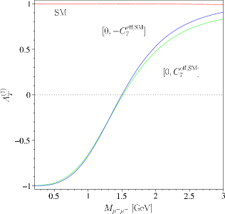
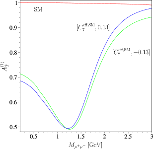
Figure 3: The transverse asymmetry $A^{(1)}_{T}$ as a function of the dimuon mass, for different choices of $[C_{7}^{\mathrm{eff}},C_{7}^{\mathrm{eff}\prime}]$. The SM prediction corresponds to the case $[C_{7}^{\mathrm{eff,SM}},0]$. We have taken into account the bound in Eq. (4.10) and the SM values for $C_{9,10}$ from Ref. [12].

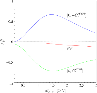
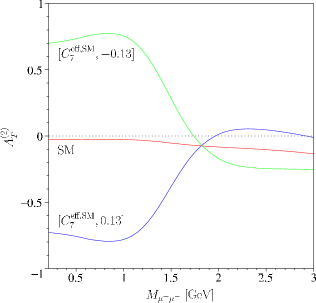
Figure 4: The asymmetry $A^{(2)}_{T}$ as a function of the dimuon mass, for different new-physics scenarios. See Fig. 3 for details.

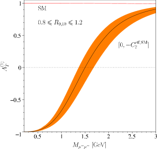
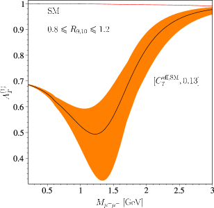
Figure 5: The asymmetry $A_{T}^{(1)}$ vs the dimuon mass for fixed $[C_{7}^{\text{eff}},{C_{7}^{\text{eff}}}^{\prime}]$, including new-physics contributions to $C_{9,10}$. The shaded areas have been obtained by varying $R_{9,10}\equiv C_{9,10}/C_{9,10}^{\mathrm{SM}}$ in a range that is consistent with present data on rare $B$ decays (see, e.g., Refs. [9, 29]). The inner solid lines correspond to the case where $C_{9,10}=C_{9,10}^{\mathrm{SM}}$.

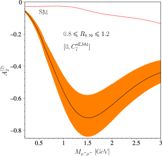
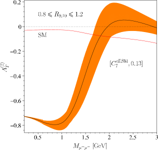
Figure 6: $A^{(2)}_{T}$ vs the dimuon mass in the presence of new-physics contributions to $C_{7}^{\mathrm{eff}(\prime)},C_{9,10}$. See Fig. 5 for details.

So far we have assumed that new physics enters only via $C_{7}^{\mathrm{eff}(\prime)}$ while the remaining coefficients are SM-like. Allowing for non-standard contributions to the coefficients $C_{9,10}$, and taking into account the constraints from rare $B$ decays [9, 29] (see also [30]), we obtain the asymmetries shown in Figs. 5 and 6. As can be seen, a determination of the magnitude of the right-handed currents is possible even in the presence of new-physics contributions to $C_{9,10}$ of the order of $20\%$. In view of this and the small theoretical uncertainties expected from our previous discussion in the SM, it is clear that the transverse asymmetries $A_{T}^{(1,2)}$ can be an especially useful probe of the electromagnetic penguin operator ${\mathcal{O}}_{7}^{\prime}$. We therefore conclude that a measurement of $A^{(1,2)}_{T}$ in the low dilepton mass region different from their SM values could be a hint of new physics with right-handed quark currents.

(ii) $\alpha_{K^{*}}$. Our results for the $K^{*}$ polarization parameter are shown in Fig. 7. Like in the case of the transverse asymmetries, new physics can give large contributions, but only for extreme scenarios. We emphasize that some of the new-physics scenarios shown in Fig. 7 are indistinguishable if we also allow $C_{9,10}$ to deviate from their SM values. Moreover, from our discussion of the SM prediction, we expect important NLL corrections to $\alpha_{K^{*}}$ in the presence of new physics and a large theoretical error due to the poorly known form factor $\xi_{\perp}(0)$.

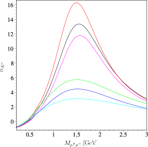
Figure 7: The $K^{*}$ polarization parameter $\alpha_{K^{*}}$ as a function of the dimuon mass for different sets of $[C_{7}^{\mathrm{eff}},C_{7}^{\mathrm{eff}\prime}]$ (from top to bottom): (i) $[C_{7}^{\mathrm{eff,SM}},0]$ (SM), (ii) $[C_{7}^{\mathrm{eff,SM}},-0.13]$, (iii) $[C_{7}^{\mathrm{eff,SM}},0.13]$, (iv) $[0,C_{7}^{\mathrm{eff,SM}}]$, (v) $[0,-C_{7}^{\mathrm{eff,SM}}]$, (vi) $[-C_{7}^{\mathrm{eff,SM}},0]$. The remaining Wilson coefficients are assumed to be SM-valued.

(iii) $F_{L,T}$. The longitudinal and transverse polarization fractions are plotted in Fig. 8 for two scenarios of $C_{7}^{\mathrm{eff}(\prime)}$. Recalling that the polarization fractions are related to the $K^{*}$ polarization parameter, $\alpha_{K^{*}}=2F_{L}/F_{T}-1$, the conclusions drawn in (ii) also apply to $F_{L,T}$ except that the uncertainty induced by the parameter $\xi_{\perp}(0)$ is smaller. As far as additional operators are concerned, we merely mention that their impact on $F_{L}/F_{T}$ was studied model-independently in Ref. [31], but for ${C_{7}^{\text{eff}}}^{\prime}=0$ and without using the soft form factor relations in Eqs. (2.8).

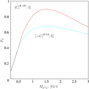
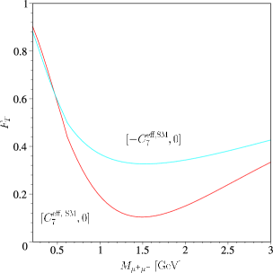
Figure 8: Longitudinal and transverse $K^{*}$ polarization fractions vs the dimuon mass, for two scenarios of $[C_{7}^{\mathrm{eff}},C_{7}^{\mathrm{eff}\prime}]$ and $C_{9,10}$ being SM-like. Since the remaining new-physics cases displayed in Fig. 7 lie between these two curves, they are not shown here.

5 Summary and conclusions

In this paper we have performed a detailed analysis of the $K^{*}$ polarization states in the decay ${B}^{0}\to K^{*0}(\to K^{-}\pi^{+})l^{+}l^{-}$. We have focused on the kinematic region in which the energy of the $K^{*}$ is of order $O(m_{b})$, so that the theoretical predictions for the heavy-to-light form factors are applicable [11, 12]. Within the framework of the SM, we have taken into account factorizable as well as non-factorizable corrections at NLL order. We have shown that the asymmetries $A_{T}^{(1,2)}$, which involve transversely polarized $K^{*}$, are largely free of hadronic uncertainties. At leading order in the heavy quark and large energy expansion, we have found that the dependence of the transverse asymmetries on the hadronic form factors completely drops out. Taking into account NLL corrections of order $\alpha_{s}$ [12], and varying the theoretical input parameters, the error on the integrated transverse asymmetries in the low dimuon mass region is found to be less than $7\%$. Within the SM, we obtain at NLL order ${\mathcal{A}}_{T}^{(1)}=0.9986\pm 0.0002$ and ${\mathcal{A}}_{T}^{(2)}=-0.043\pm 0.003$. Thus, a measurement of $A_{T}^{(1,2)}$ will allow a precise test of the SM. We have also investigated the $K^{*}$ polarization fractions in the low dimuon mass region. At NLL order, the longitudinal and transverse polarization fractions are predicted to be $(69\pm 3)\%$ and $(31\pm 3)\%$ respectively, and hence $\Gamma_{L}/\Gamma_{T}=2.23\pm 0.31$.

We further studied model-independently the implications of new physics for the $K^{*}$ polarization states. Since the low dilepton mass region is dominated by the photon pole, $|C_{7}^{\mathrm{eff}(\prime)}|^{2}/s$, we have first concentrated on such new-physics scenarios that can give appreciable contributions to the Wilson coefficients $C_{7}^{\mathrm{eff}(\prime)}$ of the electromagnetic dipole operators ${\mathcal{O}}_{7}^{(\prime)}\sim m_{b}(\bar{s}\sigma_{\mu\nu}P_{L(R)}b)F^{\mu\nu}$. Taking into account constraints on the inclusive $b\to s\gamma$ branching ratio and assuming $C_{9,10}$ being SM-like, we have found large effects on the transverse asymmetries $A_{T}^{(1,2)}$ (Figs. 3 and 4) and on the $K^{*}$ polarization parameter $\alpha_{K^{*}}$ (Fig. 7). While the former observables provide a useful tool to search for new physics, the latter still suffers from theoretical uncertainties due to the soft form factor $\xi_{\perp}(0)$ (see Fig. 2). Nevertheless, the $K^{*}$ polarization parameter will provide valuable information on non-standard physics once we have better control on the actual value of $\xi_{\perp}(0)$. We have also investigated the implications of new physics for the longitudinal and transverse polarization fractions (Fig. 8) whose measurement will allow to constrain beyond-the-SM scenarios.

In addition to the aforementioned scenario with $C_{9,10}$ being SM-valued, we have investigated the case where these coefficients receive additional contributions. Focusing on the transverse asymmetries $A_{T}^{(1,2)}$, and taking into account experimental data on rare $B$ decays, we have found that $A_{T}^{(1,2)}$ are still sensitive to the electromagnetic dipole operator ${\mathcal{O}}_{7}^{\prime}$ (Figs. 5 and 6). Thus, they provide an especially useful tool to search for right-handed currents in the low dilepton mass region.

To sum up, the study of the angular distribution of the decay ${B}^{0}\to K^{*0}(\to K^{-}\pi^{+})l^{+}l^{-}$ provides valuable information on the $K^{*}$ spin amplitudes. This enables us to probe non-standard interactions in a way that is not possible through measurements of the branching ratio and the lepton forward-backward asymmetry. Of particular interest is the lower part of the dilepton invariant mass region, where the hadronic uncertainties can be considerably reduced by exploiting the heavy-to-light form factor relations in the heavy quark and large-$E_{K^{*}}$ limit.

Appendix A Angular distribution of ${B^{0}}\to K^{*0}(\to K^{-}\pi^{+})l^{+}l^{-}$

In this appendix we give the differential decay rate formula for finite lepton mass. Assuming the $K^{*}$ to be on the mass shell, and summing over the spins of the final particles, the differential decay distribution of ${B^{0}}\to K^{*0}(\to K^{-}\pi^{+})l^{+}l^{-}$ can be written as

$$d^{4}\Gamma=\frac{9}{32\pi}I(s,\theta_{l},\theta_{K^{*}},\phi)ds\,d\cos\theta_{l}\,d\cos\theta_{K^{*}}\,d\phi,$$ (A.1)

with the physical region of phase space

$$4m_{l}^{2}\leqslant s\leqslant(m_{B}-m_{K^{*}})^{2},\quad-1\leqslant\cos\theta_{l}\leqslant 1,\quad-1\leqslant\cos\theta_{K^{*}}\leqslant 1,\quad 0\leqslant\phi\leqslant 2\pi,$$ (A.2)

and

$$I = I_{1}+I_{2}\cos 2\theta_{l}+I_{3}\sin^{2}\theta_{l}\cos 2\phi+I_{4}\sin 2\theta_{l}\cos\phi+I_{5}\sin\theta_{l}\cos\phi+I_{6}\cos\theta_{l}$$ (A.3)

$$+ I_{7}\sin\theta_{l}\sin\phi+I_{8}\sin 2\theta_{l}\sin\phi+I_{9}\sin^{2}\theta_{l}\sin 2\phi.$$

The three angles $\theta_{l},\theta_{K^{*}},\phi$, which uniquely describe the decay ${B^{0}}\to K^{*0}(\to K^{-}\pi^{+})l^{+}l^{-}$, are illustrated in Fig. 9.

Figure 9: Definition of kinematic variables in the decay ${B^{0}}\to K^{*0}(\to K^{-}\pi^{+})l^{+}l^{-}$.

Note that $\phi$ is the angle between the normals to the planes defined by $K^{-}\pi^{+}$ and $l^{+}l^{-}$ in the rest frame of the $B$ meson; that is, defining the unit vectors

$${\bf e}_{l}=\frac{{\bf p}_{l^{-}}\times{\bf p}_{l^{+}}}{|{\bf p}_{l^{-}}\times{\bf p}_{l^{+}}|},\quad{\bf e}_{K}=\frac{{\bf p}_{K^{-}}\times{\bf p}_{\pi^{+}}}{|{\bf p}_{K^{-}}\times{\bf p}_{\pi^{+}}|},\quad{\bf e}_{z}=\frac{{\bf p}_{K^{-}}+{\bf p}_{\pi^{+}}}{|{\bf p}_{K^{-}}+{\bf p}_{\pi^{+}}|},$$ (A.4)

where ${\bf p}_{i}$ denote three-momentum vectors in the $B$ rest frame, we have

$$\sin\phi=({\bf e}_{l}\times{\bf e}_{K})\cdot{\bf e}_{z},\quad\cos\phi={\bf e}_{K}\cdot{\bf e}_{l}.$$ (A.5)

The functions $I_{1-9}$ in Eq. (A.3) can be written in terms of the transversity amplitudes $A_{0}$, $A_{\|}$, ${A}_{\bot}$, $A_{t}$. The last of these corresponds to the scalar component of the virtual $K^{*}$, which is negligible if the lepton mass is small. For $m_{l}\neq 0$, we find

$$I_{1} = \bigg{\{}\frac{3}{4}[|A_{\bot L}|^{2}+|A_{\|L}|^{2}+(L\to R)]\bigg{(}1-\frac{4m_{l}^{2}}{3s}\bigg{)}+\frac{4m_{l}^{2}}{s}{\text{Re}}(A_{\bot L}A_{\bot R}^{*}+A_{\|L}A_{\|R}^{*})\bigg{\}}\sin^{2}\theta_{K^{*}}$$ (A.6a)

$$+ \bigg{\{}(|A_{0L}|^{2}+|A_{0R}|^{2})+\frac{4m_{l}^{2}}{s}[|A_{t}|^{2}+2{\text{Re}}(A_{0L}A_{0R}^{*})]\bigg{\}}\cos^{2}\theta_{K^{*}},$$

$$I_{2} = \bigg{(}1-\frac{4m_{l}^{2}}{s}\bigg{)}\bigg{[}\frac{1}{4}(|A_{\bot L}|^{2}+|A_{\|L}|^{2})\sin^{2}\theta_{K^{*}}-|A_{0L}|^{2}\cos^{2}\theta_{K^{*}}+(L\to R)\bigg{]},$$ (A.6b)

$$I_{3}=\frac{1}{2}\bigg{(}1-\frac{4m_{l}^{2}}{s}\bigg{)}\bigg{[}(|A_{\bot L}|^{2}-|A_{\|L}|^{2})\sin^{2}\theta_{K^{*}}+(L\to R)\bigg{]},$$ (A.6c)

$$I_{4}=\frac{1}{\sqrt{2}}\bigg{(}1-\frac{4m_{l}^{2}}{s}\bigg{)}\bigg{[}{\text{Re}}(A_{0L}A_{\|L}^{*})\sin 2\theta_{K^{*}}+(L\to R)\bigg{]},$$ (A.6d)

$$I_{5}=\sqrt{2}\bigg{(}1-\frac{4m_{l}^{2}}{s}\bigg{)}^{1/2}\bigg{[}{\text{Re}}(A_{0L}A_{\bot L}^{*})\sin 2\theta_{K^{*}}-(L\to R)\bigg{]},$$ (A.6e)

$$I_{6}=2\bigg{(}1-\frac{4m_{l}^{2}}{s}\bigg{)}^{1/2}\bigg{[}{\text{Re}}(A_{\|L}A_{\bot L}^{*})\sin^{2}\theta_{K^{*}}-(L\to R)\bigg{]},$$ (A.6f)

$$I_{7}=\sqrt{2}\bigg{(}1-\frac{4m_{l}^{2}}{s}\bigg{)}^{1/2}\bigg{[}{\text{Im}}(A_{0L}A_{\|L}^{*})\sin 2\theta_{K^{*}}-(L\to R)\bigg{]},$$ (A.6g)

$$I_{8}=\frac{1}{\sqrt{2}}\bigg{(}1-\frac{4m_{l}^{2}}{s}\bigg{)}\bigg{[}{\text{Im}}(A_{0L}A_{\bot L}^{*})\sin 2\theta_{K^{*}}+(L\to R)\bigg{]},$$ (A.6h)

$$I_{9}=\bigg{(}1-\frac{4m_{l}^{2}}{s}\bigg{)}\bigg{[}{\text{Im}}(A_{\|L}^{*}A_{\bot L})\sin^{2}\theta_{K^{*}}+(L\to R)\bigg{]}.$$ (A.6i)

The expression for the differential decay rate in Eq. (A.1), together with the formulae in Eqs. (A.6), agrees with the result derived in Ref. [32] for the decay $B\to D^{*}(\to D\pi)l^{+}l^{-}$ and $m_{l}\neq 0$, and with Ref. [2] in the case of massless leptons (see also Refs. [1, 3]). The differential decay rate in terms of the helicity amplitudes $H_{\pm 1},H_{0},H_{t}$ can be obtained from Eqs. (A.6) by means of the relations in Eq. (3.6).

References

- [1] D. Melikhov, N. Nikitin, and S. Simula, Phys. Lett. B 442, 381 (1998).
- [2] F. Krüger, L. M. Sehgal, N. Sinha, and R. Sinha, Phys. Rev. D 61, 114028 (2000); 63, 019901(E) (2001).
- [3] C. S. Kim, Y. G. Kim, C.-D. Lü, and T. Morozumi, Phys. Rev. D 62, 034013 (2000); C. S. Kim, Y. G. Kim, and C.-D. Lü, ibid. 64, 094014 (2001).
- [4] C.-H. Chen and C. Q. Geng, Nucl. Phys. B636, 338 (2002).
- [5] Y. Grossman and D. Pirjol, J. High Energy Phys. 0006, 029 (2000).
- [6] A. Ali and A. S. Safir, Eur. Phys. J. C 25, 583 (2002).
- [7] T. Feldmann and J. Matias, J. High Energy Phys. 0301, 074 (2003).
- [8] A. Ali, P. Ball, L. T. Handoko, and G. Hiller, Phys. Rev. D 61, 074024 (2000).
- [9] A. Ali, E. Lunghi, C. Greub, and G. Hiller, Phys. Rev. D 66, 034002 (2002).
- [10] J. Charles, A. Le Yaouanc, L. Oliver, O. Pène, and J.-C. Raynal, Phys. Rev. D 60, 014001 (1999); Phys. Lett. B 451, 187 (1999). See also M. J. Dugan and B. Grinstein, ibid. 255, 583 (1991).
- [11] M. Beneke and T. Feldmann, Nucl. Phys. B592, 3 (2001).
- [12] M. Beneke, T. Feldmann, and D. Seidel, Nucl. Phys. B612, 25 (2001).
- [13] See, for example, C. W. Bauer, S. Fleming, and M. E. Luke, Phys. Rev. D 63, 014006 (2001); C. W. Bauer, S. Fleming, D. Pirjol, and I. W. Stewart, ibid. 63, 114020 (2001); C. W. Bauer and I. W. Stewart, Phys. Lett. B 516, 134 (2001); M. Beneke, A. P. Chapovsky, M. Diehl, and T. Feldmann, Nucl. Phys. B643, 2002 (431); R. J. Hill and M. Neubert, Nucl. Phys. B657, 229 (2003); R. J. Hill, T. Becher, S. J. Lee, and M. Neubert, J. High Energy Phys. 0407, 081 (2004).
- [14] A. L. Kagan and M. Neubert, Phys. Lett. B 539 227 (2002).
- [15] A. J. Buras and M. Münz, Phys. Rev. D 52, 186 (1995); M. Misiak, Nucl. Phys. B393, 23 (1993); B439, 461(E) (1995); G. Buchalla, A. J. Buras, and M. E. Lautenbacher, Rev. Mod. Phys. 68, 1125 (1996); A. J. Buras, in Probing the Standard Model of Particle Interactions, edited by R. Gupta et al. (Elsevier Science B.V., New York, 1999), p. 281, hep-ph/9806471.
- [16] See, for example, P. Cho and M. Misiak, Phys. Rev. D 49, 5894 (1994); C. Greub, A. Ioannisian, and D. Wyler, Phys. Lett. B 346, 149 (1995); P. Ball, J. M. Frère, and J. Matias, Nucl. Phys. B572, 3 (2000).
- [17] See, for example, F. Borzumati, C. Greub, T. Hurth, and D. Wyler, Phys. Rev. D 62, 075005 (2000); T. Besmer, C. Greub, and T. Hurth, Nucl. Phys. B609, 359 (2001); L. Everett, G. L. Kane, S. Rigolin, L.-T. Wang, and T. T. Wang, J. High Energy Phys. 0201, 022 (2002).
- [18] C. Bobeth, M. Misiak, and J. Urban, Nucl. Phys. B574, 291 (2000).
- [19] H. H. Asatryan, H. M. Asatrian, C. Greub, and M. Walker, Phys. Lett. B 507, 162 (2001); Phys. Rev. D 65, 074004 (2002); 66, 034009 (2002); A. Ghinculov, T. Hurth, G. Isidori, and Y. P. Yao, Nucl. Phys. B648, 254 (2003).
- [20] P. Gambino, M. Gorbahn, and U. Haisch, Nucl. Phys. B673, 238 (2003); C. Bobeth, P. Gambino, M. Gorbahn, and U. Haisch, J. High Energy Phys. 0404, 071 (2004).
- [21] M. Wirbel, B. Stech, and M. Bauer, Z. Phys. C 29, 637 (1985); B. Stech, ibid. 75, 245 (1997).
- [22] G. Burdman and G. Hiller, Phys. Rev. D 63, 113008 (2001).
- [23] B. Stech, Phys. Lett. B 354, 447 (1995); J. M. Soares, Phys. Rev. D 54, 6837 (1996); hep-ph/9810402.
- [24] J. M. Soares, hep-ph/9810421.
- [25] D. Chang, A. Masiero, and H. Murayama, Phys. Rev. D 67, 075013 (2003).
- [26] A. Ali and A. Y. Parkhomenko, Eur. Phys. J. C 23, 89 (2002); S. W. Bosch and G. Buchalla, Nucl. Phys. B621, 459 (2002).
- [27] K. G. Chetyrkin, M. Misiak, and M. Münz, Phys. Lett. B 400, 206 (1997); 425, 414(E) (1998); P. Gambino and M. Misiak, Nucl. Phys. B611, 338 (2001); A. J. Buras, A. Czarnecki, M. Misiak, and J. Urban, ibid. B631, 219 (2002).
- [28] CLEO Collaboration, S. Chen et al., Phys. Rev. Lett. 87, 251807 (2001); BaBar Collaboration, B. Aubert et al., hep-ex/0207076; Belle Collaboration, P. Koppenburg et al., Phys. Rev. Lett. 93, 061803 (2004); Heavy Flavor Averaging Group, http://www.slac.stanford.edu/xorg/hfag.
- [29] G. Hiller and F. Krüger, Phys. Rev. D 69, 074020 (2004).
- [30] P. Gambino, U. Haisch, and M. Misiak, hep-ph/0410155.
- [31] T. M. Aliev, C. S. Kim, and Y. G. Kim, Phys. Rev. D 62, 014026 (2000).
- [32] A. Faessler, T. Gutsche, M. A. Ivanov, J. G. Körner, and V. E. Lyubovitskij, EPJdirect C4, 18 (2002).