Pre-critical Phenomena of Two-flavor Color Superconductivity in Heated Quark Matter

Abstract

We investigate the fluctuations of the diquark-pair field and their effects on observables above the critical temperature $T_{c}$ in two-flavor color superconductivity (CSC) at moderate density using a Nambu-Jona-Lasinio-type effective model of QCD. Because of the strong-coupling nature of the dynamics, the fluctuations of the pair field develop a collective mode, which has a prominent strength even well above $T_{c}$. We show that the collective mode is actually the soft mode of CSC. We examine the effects of the pair fluctuations on the specific heat and the quark spectrum for $T$ above but close to $T_{c}$. We find that the specific heat exhibits singular behavior because of the pair fluctuations, in accordance with the general theory of second-order phase transitions. The quarks display a typical non-Fermi liquid behavior, owing to the coupling with the soft mode, leading to a pseudo-gap in the density of states of the quarks in the vicinity of the critical point. Some experimental implications of the precursory phenomena are also discussed.

1 Introduction

In recent years, there have been many studies of the properties of dense and cold matter[1]. In such a system, the baryonic density is so high that quarks and gluons are expected to be deconfined to make a quark matter[2]. Then, the attractive quark-quark interaction in some channels should give rise to a Cooper instability leading to color superconductivity (CSC) at sufficiently low temperatures[3, 4]. The asymptotic freedom of QCD allows us to use perturbation theory to describe CSC at extremely high densities with $\mu>10^{8}$ MeV, where $\mu$ is the quark chemical potential[5]. In this region, the weak-coupling theory analogous to BCS theory, i.e. a mean-field approximation (MFA), is valid. In such a system composed of u, d and s quarks at extremely high density, it is believed that the quark matter takes the special form of the color-superconducting phase, i.e. the color-flavor locked (CFL) phase,[6] in which all kinds of quarks take part equally in the pairing.

What is the phenomenological significance of CSC including the CFL? Possible relevant systems consisting dense QCD matter include the cores of compact stars,[7] both in equilibrium and in the newly-born stage and the intermediated states created in the heavy-ion collisions that are expected to be performed in the forthcoming facilities at GSI and J-PARC[8, 9]. One of the basic points concerning real systems of this kind lies in the fact that the quark-number chemical potential $\mu$ and hence the baryon density are moderate; $\mu$ should be at most $\sim$500 MeV. Therefore the ideal situation realized in an extremely dense system may not be expected in these real systems but various complications come into play in the determination of the nature of CSC.

To realize CSC in a compact star at vanishing temperature, the color- and electric-charge neutrality conditions must be satisfied as well as the $\beta$-equilibrium condition.[10, 11, 12] These conditions, in turn, induce a mismatch of the Fermi momenta of quarks of different flavors and colors. This is the case in particular when the constituent mass of the strange quark, $M_{s}$ (which ranges from some 100 to 500 MeV owing to the dynamical symmetry breaking of the chiral symmetry) is comparable with $\mu$. Thus we see that the incorporation of the charge neutrality and $\beta$-equilibrium conditions, with finite $M_{s}$ taken into account, brings about quite interesting complications in the physics of CSC in quark matter at moderate densities. Indeed, it has been shown in the MFA that the combination of all these effects can lead to a variety of pairing patterns, including the so-called gapless CFL’s [13, 14, 15, 16, 17, 18, 19, 20].

In this paper, we focus on another important feature of QCD matter at moderate densities, i.e. the strong-coupling nature of QCD at low energy scales, which invalidates the MFA. This strong coupling may imply the significance of large fluctuations of the diquark-pair field, especially in the vicinity of the critical temperature, $T_{c}$[8, 21, 22]. It is noteworthy that some recent analyses of the RHIC experiments suggest that quasi-bound quark-antiquark states may be formed in moderately hot QCD matter. This reflects the strong-coupling nature of QCD[23], although the possible existence of hadronic modes above $T_{c}$ was suggested earlier in Refs. ref:HK85 and ref:DeTar85 .

It is thus natural to expect that heated quark matter at a moderate density may also accommodate pre-formed diquark pairs as a pre-critical phenomenon of CSC phase transition. Owing to the strong-coupling nature inducing large fluctuations of the order parameter, CSC in heated quark matter at moderate densities may have some of the same basic properties as the superconductivity in strongly correlated electron systems, such as high-$T_{c}$ superconductivity(HTSC), rather than usual superconductivity in metals. [8, 27] We notice that materials at $T>T_{c}$ show various types of non-Fermi liquid behavior, one of which is pseudogap formation, i.e. an anomalous depression of the density of states (DOS) $N(\omega)$ as a function of the fermion energy $\omega$ around the Fermi surface[28, 29, 30]. It would be intriguing to explore whether quarks in the heated quark matter near the critical point exhibit similar abnormal behavior. In this paper, we investigate pair fluctuations of CSC for $T$ above $T_{c}$ and explore their effects on some physical quantities, including the quark spectra in such quark matter near the critical point.

The relevant quark matters we have in mind are those created by the heavy-ion collisions or those realized in the core of a proto-compact star just after a supernova explosion. In these systems, the temperature is considerably high, and for this reason the $\beta$-equilibrium condition may not be completely satisfied, in contrast to the case in the interiors of cold compact stars. Therefore, the difference between the chemical potentials of the up- and down-quarks in these systems is smaller than that under the $\beta$-equilibrium condition, and hence a two-flavor superconductor (2SC) will be favored over other pairings which incorporate strange quarks. Furthermore, the effect of the difference in chemical potentials induced by the neutrality conditions will be smaller at finite temperature than that at $T=0$, because the Fermi surface is diffused for $T\not=0$[15]. Thus, one may simply introduce the same chemical potential for all the kinds of quarks as a fair approximation to study CSC in such hot quark matter.

There are two types of fluctuations in superconductors, i.e., the fermion-pair and gauge-field fluctuations, irrespective of whether they are electric or color superconductors. Gauge-field fluctuations are known to make CSC phase transition first order in the weak coupling region[4, 31, 32, 33]. In this region, it is known that CSC is strong type-I superconductivity[31, 34] in which the fluctuations of the gauge field dominate the pair-field fluctuations. On the other hand, as is argued in Ref. ref:GR03, CSC is expected to be type-II superconductivity at lower density, i.e. for $\mu\lesssim 500$MeV, where the fluctuations of the pair field dominate those of the gauge field in contrast to the weak-coupling case. In the present work, therefore, we simply ignore the gluon degrees of freedom, and examine the effects of pair fluctuations near $T_{c}$, as done in Refs. ref:KKKN1 and ref:KKKN3: Because pair fluctuations are inherent in second- (or weak first-) order phase transitions, the results in the present work should hold irrespective of the different pairing patterns and the chemical potential combination, as long as the phase transition to CSC is second order or weak first order. We treat the system at relatively low density, where the strange quark degrees of freedom do not come into play; accordingly the pairing pattern is taken as 2SC throughout this paper.

To investigate a system at relatively low temperature and density, a perturbative QCD calculation is inadequate, because of the strong coupling. Lattice Monte Carlo simulations for finite $\mu$ are still immature for the present purpose, although much progress has been being made in recent years[35]. Therefore, it is appropriate to adopt a low-energy effective theory of QCD. Because we are considering the situation in which the diquark pairing dominates over that of the gluons, an effective model composed solely of the quark fields may be adopted. Such effective models include the instanton induced model[36] and the Nambu-Jona-Lasinio (NJL) model[37, 38]. Note that the latter model is a simplified version of the former. Both models are in fact used to explore the phase structure at low density [38, 39, 40, 41, 42]. One should note here that an NJL-type theory can be deduced as a low-energy effective theory for dense quark matter on the basis of the renormalization-group equations[43]. It is also known that the phase structures obtained in these models are qualitatively consistent, and they are similar to those calculated using the Schwinger-Dyson equation with the one-gluon exchange interaction[22, 44]. In this work, we employ the NJL model to explore the fluctuations in CSC.

In previous short communications, Refs. ref:KKKN1 and ref:KKKN3, we studied the precursory phenomena to CSC: We showed for a vanishing wave number that the dynamical fluctuations of the pair field have a prominent strength near the vanishing frequency up to $T\simeq 1.2T_{c}$ [8], and for this reason that these fluctuations can give rise to interesting precursory phenomena, such as a pseudogap in the quark DOS near $T_{c}$.[27] It is worth emphasizing that Ref. ref:KKKN3 is the first investigation to explore whether and how the quasi-particle properties of quarks are changed by the precursory paring mode in CSC. In the present paper, we present a formulation of the basic theory and give a detailed account of both analytic and numerical calculational procedures. We also present a more extensive study of the properties of the precursory pair field with finite wave-numbers and the mechanism through which the pseudogap appears. We investigate for the first time the effects of the precursory pair fluctuations on the specific heat. It is found that the heated quark matter close to the critical point of CSC shows typical non-Fermi liquid behavior, owing to the precursory pair fluctuations, which form a soft mode.

This paper is organized as follows. In §2, we introduce our model Lagrangian and present the phase diagram obtained in the MFA in the model. In §3, we investigate the behavior of the pair fluctuations above $T_{c}$ using linear response theory. It is shown that the fluctuations of the pair field develop a collective mode with a large strength even well above $T_{c}$. We show that the complex frequency of the collective pair-field moves toward the origin in the complex energy plane, which implies that the pair fluctuations form the soft mode of CSC phase transition. We calculate the spectral function of the pair fluctuations, $\rho(\mbox{{\boldmath$k$}},\omega)$, as a function of the momentum $k$ and energy $\omega$ in order to elucidate the spatial and temporal behavior of the pair fluctuations when the temperature is lowered toward $T_{c}$. We also present the behavior of the dynamical structure factor. In §4, we discuss the effect of the soft mode on the specific heat $c_{\rm v}$ above $T_{c}$ and show that $c_{\rm v}$ increases when $T$ is lowered to $T_{c}$ and eventually diverges at $T=T_{c}$ in accordance with the singular growth of pair fluctuations. We examine how the soft mode affects the single quark spectrum and changes the quasi-particle picture of the fermion above $T_{c}$ in §5. We start from a calculation of the single-quark Green function in the T-matrix approximation to incorporate the effects of the pair fluctuations in the quark sector. It is shown that the pair fluctuations give rise to a large decay width for quarks near the Fermi surface, i.e. non-Fermi liquid behavior of the quarks near $T_{c}$. It is further shown that the anomalous behavior leads to a pseudogap in the DOS of the quarks. The chemical potential dependences of the quark spectrum and the DOS are also examined. The final section is devoted to a summary and concluding remarks.

2 Model and Phase Diagram

In this section, after introducing our model Lagrangian, we recapitulate the derivation of the thermodynamic potential and present the phase diagram obtained in the MFA[41]. This forms the basis for the succeeding investigation of the nature of the precursory pair fluctuations.

We employ a Nambu–Jona-Lasinio (NJL) model with two flavors and three colors, as mentioned in the Introduction:

$${\cal L}=\bar{\psi}i/\partial\psi+{\cal L}_{S}+{\cal L}_{C}.$$ (1)

Here the quark-antiquark and quark-quark interactions, ${\cal L}_{S}$ and ${\cal L}_{C}$ are given by

$${\cal L}_{S} = G_{S}[(\bar{\psi}\psi)^{2}+(\bar{\psi}i\gamma_{5}\vec{\tau}\psi)^{2}],$$

$${\cal L}_{C} = G_{C}(\bar{\psi}i\gamma_{5}\tau_{2}\lambda_{A}\psi^{C})(\bar{\psi}^{C}i\gamma_{5}\tau_{2}\lambda_{A}\psi),$$ (2)

with $\psi^{C}(\mbox{{\boldmath$x$}})\equiv C\bar{\psi}^{T}(\mbox{{\boldmath$x$}})$ and $C=i\gamma_{2}\gamma_{0}$ being the charge conjugation operator. The matrices $\tau_{2}$ and $\lambda_{A}$ $(A=2,5,7)$ are the antisymmetric components of the Pauli and Gell-Mann matrices for the flavor $SU(2)_{f}$ and color $SU(3)_{c}$, respectively. We take the chiral limit putting $m_{u}=m_{d}=0$, since the properties of the diquark condensates are affected very little by the small quark masses.

We choose the scalar coupling constant as $G_{S}=5.01\,{\rm GeV}^{-2}$ and the three-dimensional momentum cutoff $\Lambda=650$MeV so as to reproduce the pion decay constant $f_{\pi}=93$ MeV and the chiral condensate $\langle\bar{\psi}\psi\rangle=(-250{\rm MeV})^{3}$ in the chiral limit[46]. There are several sources to determine the diquark coupling constant $G_{C}$, for example, the instanton-induced interaction and the diquark-quark picture of baryons[47]. The former gives $G_{C}/G_{S}=0.5$[42], while the values $G_{C}/G_{S}=0.49-0.73$[48] and $G_{C}/G_{S}=1.5-2$[49] have been obtained using the latter model. In the present work we fix $G_{C}/G_{S}$=0.62, i.e., $G_{C}=3.11\,{\rm GeV}^{-2}$, following Refs. ref:SKP,ref:KKKN1 and ref:KKKN3, where $G_{C}$ is chosen so as to reproduce phase diagram similar to that calculated in the instanton-induced interaction[39].

To determine the phase diagram, we have to first derive the thermodynamic potential $\Omega=-T\log{\rm Tr}~{}{\rm e}^{-\beta K}$ with

$$K=\int d^{3}\mbox{{\boldmath$x$}}\left\{\bar{\psi}(-i\mbox{{\boldmath$\gamma$}}\cdot\vec{\nabla})\psi-\mu\bar{\psi}\gamma^{0}\psi-{\cal L}_{S}-{\cal L}_{C}\right\}.$$ (3)

Here, Tr denotes a trace operation over the color, flavor and Dirac indices. To apply the MFA, we assume a finite diquark condensate for the 2SC pairing $\Delta$ and the quark-antiquark condensate $M$,

$$\Delta=-2G_{C}\langle\bar{\psi}^{C}\Gamma\psi\rangle,\qquad M=-2G_{S}\langle\bar{\psi}\psi\rangle,$$ (4)

with $\Gamma\equiv i\gamma_{5}\tau_{2}\lambda_{2}$. Employing the MFA for ${\cal L}_{C}$ and ${\cal L}_{S}$, the thermodynamic potential in the MFA per unit volume is given by[41]

$$\Omega_{MF}(M,\Delta;T,\mu) = -\frac{T}{V}\log{\rm Tr}{\rm e}^{-\beta K}$$ (5)

$$= \frac{M^{2}}{4G_{S}}+\frac{|\Delta|^{2}}{4G_{C}}-4\int\frac{d^{3}p}{(2\pi)^{3}}\left\{E_{p}+T\log\left(1+{\rm e}^{-\beta\xi_{-}}\right)\left(1+{\rm e}^{-\beta\xi_{+}}\right)\right.$$

$$\left.+\epsilon_{-}+\epsilon_{+}+2T\log\left(1+{\rm e}^{-\beta\epsilon_{-}}\right)\left(1+{\rm e}^{-\beta\epsilon_{+}}\right)\right\},$$

where

$$E_{p}=\sqrt{p^{2}+M^{2}},\qquad\xi_{\pm}=E_{p}\pm\mu,\qquad\epsilon_{\pm}=\sqrt{\xi^{2}_{\pm}+|\Delta|^{2}},$$ (6)

and $\beta=1/T$. The thermodynamic potential $\Omega_{MF}$ realizes its absolute minimum as a function of $M$ and $\Delta$ in the equilibrium state; accordingly the optimal values of $M$ and $\Delta$ satisfy the stationary conditions

$$\frac{\partial\Omega_{MF}}{\partial M}\biggl{|}_{\Delta}=0\qquad{\rm and}\qquad\frac{\partial\Omega_{MF}}{\partial\Delta}\biggl{|}_{M}=0,$$ (7)

which are actually self-consistent equations for the condensates and are called “the gap equations”.

Using Eqs. (5) and (7), we can determine the phase structure of the model. The phase diagram in the $T$-$\mu$ plane is shown in Fig. 1: The dashed (solid) curves denote the critical line for a second-(first-)order phase transition. The critical chemical potential for the chiral-to-CSC transition at $T=0$ is $\mu=316$ MeV in our model. The second order normal-to-2SC phase transition occurs somewhere in the range $T=35-60$ MeV for $\mu=350-500$ MeV. In the following sections, we explore the pair fluctuations and precursory phenomena above $T_{c}$ in this region of $\mu$.

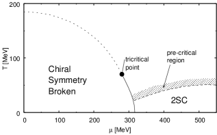
Figure 1: The calculated phase diagram in the $T$-$\mu$ plane for our model. The solid and dashed curves denote the critical lines of a first- and second-order phase transitions, respectively.

For later convenience, we now explicitly write down the critical condition for the normal-to-CSC phase transition with vanishing chiral condensate ($M=0$). We first give the explicit expression of the gap equation for $\Delta$ in Eq. (7):

$$\Delta = 8G_{C}\Delta\int\frac{d^{3}p}{(2\pi)^{3}}\left\{\frac{1}{\epsilon_{-}}\tanh\frac{\beta\epsilon_{-}}{2}+\frac{1}{\epsilon_{+}}\tanh\frac{\beta\epsilon_{+}}{2}\right\},$$ (8)

where $\epsilon_{\pm}=\sqrt{|p\pm\mu|^{2}+|\Delta|^{2}}$, because we have set $M=0$. Dividing Eq. (8) by $\Delta$ and then setting $\Delta=0$, the condition for determining the critical temperature $T_{c}$ of the normal-to-CSC phase transition is obtained as

$$0 = 1-8G_{C}\int\frac{d^{3}p}{(2\pi)^{3}}\left\{\frac{1}{p-\mu}\tanh\frac{\beta_{c}(p-\mu)}{2}+\frac{1}{p+\mu}\tanh\frac{\beta_{c}(p+\mu)}{2}\right\},$$ (9)

with $\beta_{c}\equiv 1/T_{c}$. Below we find that Eq. (9) plays a crucial role for understanding the anomalous behavior of the pair fluctuations near the critical point.

3 Pair fluctuations above $T_{c}$

In this section, we discuss the properties of the precursory fluctuations of the diquark-pair field in the normal phase on the basis of linear response theory. Because we limit our attention to the behavior of fluctuations in the normal phase, we set $M=\Delta=0$. It will be shown that a collective mode corresponding to pair fluctuations is developed near the critical point; we find that this mode is the soft mode for the CSC phase transition in the sense that the pole of the spectral function in the complex energy plane moves toward the origin as $T$ is lowered toward $T_{c}$. We then calculate the spectral function and the structural factor of the pair field with finite energy and momentum and examine their temperature dependence. We also discuss how the chemical potential $\mu$ affects the properties of the soft mode.

3.1 Linear response of the pair field

In this subsection, we apply linear response theory in order to investigate the diquark-pair fluctuations[8]. The presentation of the theory here is more formal than that given in Ref. ref:KKKN1. See also Ref. ref:KKKN1 for a more intuitive discussion of the linear response of the pair field.

When we apply an external perturbation $H_{ex}(t)$ to a thermal equilibrium state at $t=t_{0}$, the expectation value of an arbitrary operator, $\langle O(\mbox{{\boldmath$x$}},t)\rangle$, deviates from the initial equilibrium value $\langle O(\mbox{{\boldmath$x$}},t)\rangle_{eq}$, where $O(\mbox{{\boldmath$x$}},t)\equiv{\rm e}^{iKt}O(\mbox{{\boldmath$x$}}){\rm e}^{-iKt}$, with $K$ being a time-independent operator. In the linear response theory, this deviation is given by

$$\langle O(\mbox{{\boldmath$x$}},t)\rangle-\langle O(\mbox{{\boldmath$x$}},t)\rangle_{eq}=i\int^{t}_{t_{0}}ds\langle[H_{ex}(s),O(\mbox{{\boldmath$x$}},t)]\rangle_{eq}.$$ (10)

Here, $\langle~{}~{}~{}\rangle_{eq}$ represents the thermal expectation value without $H_{ex}(t)$.

In order to study the pair fluctuations of CSC, we choose

$$O(\mbox{{\boldmath$x$}}) = -2G_{C}\bar{\psi}(\mbox{{\boldmath$x$}})\Gamma\psi^{C}(\mbox{{\boldmath$x$}}),$$ (11)

$$H_{ex}(t) = \int d^{3}\mbox{{\boldmath$x$}}\Delta^{*}_{ex}(\mbox{{\boldmath$x$}},t)\left(\bar{\psi}^{C}(\mbox{{\boldmath$x$}})\Gamma\psi(\mbox{{\boldmath$x$}})\right)+h.c.,$$ (12)

where $\Delta^{*}_{ex}(\mbox{{\boldmath$x$}},t)$ is a classical external source. Substituting these into Eq. (10) and using the fact that $\langle\bar{\psi}\Gamma\psi^{C}\rangle_{eq}$ vanishes in the normal phase, we obtain the diquark pair field induced by $\Delta^{*}_{ex}$,

$$\Delta^{*}_{ind}(\mbox{{\boldmath$x$}},t) \equiv -2G_{C}\langle\bar{\psi}^{C}(\mbox{{\boldmath$x$}},t)\Gamma\psi(\mbox{{\boldmath$x$}},t)\rangle,$$ (13)

$$= -2G_{C}\int^{\infty}_{-\infty}dt^{\prime}\int d^{3}{\mbox{{\boldmath$x$}}}^{\prime}D^{R}({\mbox{{\boldmath$x$}}},t;{\mbox{{\boldmath$x$}}}^{\prime},t^{\prime})\Delta^{*}_{ex}({\mbox{{\boldmath$x$}}}^{\prime},t^{\prime}).$$

Here, the response function $D^{R}$ is given by

$$D^{R}(\mbox{{\boldmath$x$}},t;\mbox{{\boldmath$x$}}^{\prime},t^{\prime}) = -i\theta(t-t^{\prime})\langle[\bar{\psi}({\mbox{{\boldmath$x$}}},t)\Gamma\psi^{C}({\mbox{{\boldmath$x$}}},t),\bar{\psi}^{C}({\mbox{{\boldmath$x$}}}^{\prime},t^{\prime})\Gamma\psi({\mbox{{\boldmath$x$}}}^{\prime},t^{\prime})]\rangle_{eq},$$ (14)

$$= \int\frac{d^{3}{\mbox{{\boldmath$k$}}}d\omega}{(2\pi)^{4}}D^{R}(\mbox{{\boldmath$k$}},\omega){\rm e}^{-i\omega(t-t^{\prime})}{\rm e}^{i{\bf k}\cdot({\bf x}-{\bf x}^{\prime})},$$

where we have taken the limit $t_{0}\to-\infty$. The Fourier transformation of Eq. (13) gives

$$\Delta^{*}_{ind}(\mbox{{\boldmath$k$}},\omega)=-2G_{C}D^{R}(\mbox{{\boldmath$k$}},\omega)\Delta^{*}_{ex}(\mbox{{\boldmath$k$}},\omega).$$ (15)

Equation (15) contains a significant amount of information regarding elementary excitations in the system. We first note that if the external field has the form

$$\Delta^{*}_{ex}(\mbox{{\boldmath$x$}},t)=\Delta^{*}_{ex}(\mbox{{\boldmath$k$}},\omega){\rm e}^{-i\omega t+i{\bf k}\cdot{\bf x}},$$ (16)

then Eq. (15) implies that there appears an induced pair field

$$\Delta^{*}_{ind}(\mbox{{\boldmath$x$}},t)=\Delta^{*}_{ind}(\mbox{{\boldmath$k$}},\omega){\rm e}^{-i\omega t+i{\bf k}\cdot{\bf x}}$$ (17)

with amplitude $\Delta^{*}_{ind}(\mbox{{\boldmath$k$}},\omega)$. If the system has an intrinsic collective excitation with the dispersion relation $\omega=\omega_{s}(\mbox{{\boldmath$k$}})$, the induced pair field will have a larger amplitude $\Delta^{*}_{ind}(\mbox{{\boldmath$k$}},\omega)$ for $\omega\sim\omega_{s}(\mbox{{\boldmath$k$}})$ owing to a resonance mechanism; this implies that $D^{R}(\mbox{{\boldmath$k$}},\omega)$ increases as $\omega$ approaches $\omega_{s}(\mbox{{\boldmath$k$}})$ on account of Eq. (15) and eventually may diverge at $\omega=\omega_{s}(\mbox{{\boldmath$k$}})$. Conversely, if the amplitude $\Delta^{*}_{ind}(\mbox{{\boldmath$k$}},\omega)$ has a finite value with an infinitesimally-small external disturbance $\Delta^{*}_{ex}(\mbox{{\boldmath$k$}},\omega)$, the system would have an intrinsic collective excitation with frequency $\omega$ and wave number $k$. This situation is realized when the response function $D^{R}(\mbox{{\boldmath$k$}},\omega)$ is divergent, which may occur for a special $\omega$ with a given $k$. Thus we find that the equation

$${D^{R}(\mbox{{\boldmath$k$}},\omega)}^{-1}=0$$ (18)

gives the dispersion relation $\omega=\omega_{s}(\mbox{{\boldmath$k$}})$ of the possible collective excitation in the diquark channel of the system. A remark is in order. Note that the frequency $\omega_{s}(\mbox{{\boldmath$k$}})$ with given $k$ can be a complex number; for instance, (i) if Re $\omega_{s}(\mbox{{\boldmath$k$}})\not=0$, the mode is oscillatory, and (ii) if $\omega_{s}(\mbox{{\boldmath$k$}})$ is pure-imaginary, the mode is diffusive. Below we find that Re $\omega_{s}(\mbox{{\boldmath$k$}})$ is finite, but so small that the mode is almost diffusive.

The information concerning the strength of the pair fluctuations is contained in the spectral function $\rho(\mbox{{\boldmath$k$}},\omega)$, which is defined through the response function $D^{R}(\mbox{{\boldmath$k$}},\omega)$:

$$\rho(\mbox{{\boldmath$k$}},\omega)=-\frac{1}{\pi}\mbox{Im}D^{R}(\mbox{{\boldmath$k$}},\omega).$$ (19)

The strength of the fluctuations is also represented by the dynamical structure factor, defined by

$$S(\mbox{{\boldmath$k$}},\omega) = -\frac{1}{\pi(1-{\rm e}^{-\beta\omega})}{\rm Im}~{}D^{R}(\mbox{{\boldmath$k$}},\omega),$$ (20)

which is positive definite. At finite temperature, $S(\mbox{{\boldmath$k$}},\omega)$ can be directly observed in scattering experiments[50]; the van Hove scattering formula[50] gives the cross section in terms of the dynamical structure factor. As we see below, $\rho(\mbox{{\boldmath$k$}},\omega)$ represents the total width of the fluctuations, i.e., the difference between the decay rate and the production rate, and it is negative in the case $\omega<0$ for bosonic excitations. Accordingly, $S(\mbox{{\boldmath$k$}},\omega)$, not $\rho(\mbox{{\boldmath$k$}},\omega)$, represents the excitation probability of the fluctuations of the system at finite temperature.

To calculate $D^{R}(\mbox{{\boldmath$k$}},\omega)$, we employ the imaginary time formalism; we first calculate the response function in the imaginary time formalism (the two-particle Matsubara Green function),

$${\cal D}(\mbox{{\boldmath$x$}},\tau;{\bf 0},0) = -\langle T_{\tau}\bar{\psi}(\mbox{{\boldmath$x$}},\tau)\Gamma\psi^{C}(\mbox{{\boldmath$x$}},\tau)\bar{\psi}^{C}({\bf 0},0)\Gamma\psi({\bf 0},0)\rangle$$ (21)

$$\equiv T\sum_{n}\int\frac{d^{3}\mbox{{\boldmath$k$}}}{(2\pi)^{3}}{\cal D}(\mbox{{\boldmath$k$}},\nu_{n}){\rm e}^{-i\nu_{n}\tau}{\rm e}^{i{\bf k\cdot x}},$$

with $\nu_{n}=2\pi n/\beta$ being the Matsubara frequency for bosons.

Figure 2: The diquark propagator in the random phase approximation.

In order to evaluate Eq. (21), we employ the random phase approximation (RPA) in which we sum up the ring diagrams shown in Fig. 2, with the lines representing the free Matsubara Green function in the normal phase ($M=\Delta=0$),

$${\cal G}_{0}(\mbox{{\boldmath$k$}},\omega_{n})=\frac{1}{(i\omega_{n}+\mu)\gamma_{0}-\mbox{{\boldmath$k$}}\cdot\mbox{{\boldmath$\gamma$}}},$$ (22)

and the vertices correspond to ${\cal L}_{C}$. In this approximation, the Matsubara Green function (21) is given by

$${\cal D}(\mbox{{\boldmath$k$}},\nu_{n})=\frac{1}{2}\frac{{\cal Q}(\mbox{{\boldmath$k$}},\nu_{n})}{1+G_{C}{\cal Q}(\mbox{{\boldmath$k$}},\nu_{n})},$$ (23)

where ${\cal Q}(\mbox{{\boldmath$k$}},\nu_{n})$ is the contribution from the one-loop particle-particle correlation function,

$${\cal Q}(\mbox{{\boldmath$k$}},\nu_{n})=-2T\sum_{m}\int\frac{d^{3}\mbox{{\boldmath$p$}}}{(2\pi)^{3}}\mbox{Tr}\left[C\Gamma{\cal G}_{0}(\mbox{{\boldmath$k$}}-\mbox{{\boldmath$p$}},\nu_{n}-\omega_{m})\Gamma C{\cal G}_{0}^{T}(\mbox{{\boldmath$p$}},\omega_{m})\right].$$

(24)

Here $\omega_{n}=(2n+1)\pi/\beta$ denotes the Matsubara frequency for fermions. The response function in the real time Eq. (14) is given by the analytic continuation $i\nu_{n}\to\omega+i\eta$, and we obtain

$$\left.D^{R}(\mbox{{\boldmath$k$}},\omega)={\cal D}(\mbox{{\boldmath$k$}},\nu_{n})\right|_{i\nu_{n}=\omega+i\eta}=\frac{1}{2}\frac{Q^{R}(\mbox{{\boldmath$k$}},\omega)}{1+G_{C}Q^{R}(\mbox{{\boldmath$k$}},\omega)},$$ (25)

with $Q^{R}(\mbox{{\boldmath$k$}},\omega)={\cal Q}(\mbox{{\boldmath$k$}},\nu_{n})|_{i\nu_{n}=\omega+i\eta}$. It is thus seen that the equation to determine the dispersion relation for the collective excitation given in Eq. (18) is reduced to

$$1+G_{C}Q^{R}(\mbox{{\boldmath$k$}},\omega)=0.$$ (26)

With some manipulations (see Appendix A for details), we find the following simplified form of $Q^{R}(\mbox{{\boldmath$k$}},\omega)$:

$$Q^{R}(\mbox{{\boldmath$k$}},\omega) = N_{f}(N_{c}-1)\int\frac{d^{3}\mbox{{\boldmath$p$}}}{(2\pi)^{3}}\frac{1}{e_{1}e_{2}}$$

$$\times \left\{\left[(e_{1}+e_{2})^{2}-k^{2}\right]\left(\frac{1-f^{-}(e_{2})-f^{-}(e_{1})}{\omega+2\mu-e_{1}-e_{2}+i\eta}+\frac{1-f^{+}(e_{2})-f^{+}(e_{1})}{\omega+2\mu+e_{1}+e_{2}+i\eta}\right)\right.$$

$$- \left.\left[(e_{1}-e_{2})^{2}-k^{2}\right]\left(\frac{f^{-}(e_{2})-f^{+}(e_{1})}{\omega+2\mu+e_{1}-e_{2}+i\eta}+\frac{f^{+}(e_{2})-f^{-}(e_{1})}{\omega+2\mu-e_{1}+e_{2}+i\eta}\right)\right\}.$$

(27)

Here $f^{\pm}(x)=1/[{\rm e}^{\beta(x\pm\mu)}+1]$ is the Fermi-Dirac distribution function for the quark and anti-quark, respectively, and $e_{1}\equiv|\mbox{{\boldmath$p$}}|$, $e_{2}\equiv|\mbox{{\boldmath$k$}}-\mbox{{\boldmath$p$}}|$ and $k\equiv|\mbox{{\boldmath$k$}}|$. The imaginary part of $Q^{R}(\mbox{{\boldmath$k$}},\omega)$ is given by

$$\mbox{Im}Q^{R}(\mbox{{\boldmath$k$}},\omega) = -\pi N_{f}(N_{c}-1)\int\frac{d^{3}\mbox{{\boldmath$p$}}}{(2\pi)^{3}}\frac{(\omega+2\mu)^{2}-k^{2}}{e_{1}e_{2}}$$ (28)

$$\times \left[\left(1-f^{-}(e_{1})-f^{-}(e_{2})\right)\right.\delta(\omega+2\mu-e_{1}-e_{2})$$

$$-\left(1-f^{+}(e_{1})-f^{+}(e_{2})\right)\delta(\omega+2\mu+e_{1}+e_{2})$$

$$+\left(f^{-}(e_{1})-f^{+}(e_{2})\right)\delta(\omega+2\mu-e_{1}+e_{2})$$

$$\left.-\left(f^{+}(e_{1})-f^{-}(e_{2})\right)\delta(\omega+2\mu+e_{1}-e_{2})\right].$$

Each term in the square brackets of Eq. (28) corresponds to the decay process shown in Figs. 3 (a)-(d) and its inverse. To see this, the following identities for arbitrary quantities $f_{i}$ ($i=1,2$) are useful: $1-f_{1}-f_{2}=(1-f_{1})(1-f_{2})-f_{1}f_{2}$ and $f_{1}-f_{2}=(1-f_{2})f_{1}-f_{2}(1-f_{1})$. In general, the imaginary part of the retarded Green function is related to the net decay rate or the total width. Because of the delta function in each term owing to energy-momentum conservation, the ranges of energy and momentum over which each decay process can take place are restricted to the region shown in the right panel of Fig. 3; for example, the decay process into two particles, as shown in (a) of Fig. 3, and its inverse occur only for $\omega>|\mbox{{\boldmath$k$}}|-2\mu$. The processes (b) and (c), the so-called Landau damping processes, and their inverses take place only for $-|\mbox{{\boldmath$k$}}|-2\mu<\omega<|\mbox{{\boldmath$k$}}|-2\mu$; hence the collective modes with vanishing momenta do not decay through these processes. We now see that the decay process (a) plays the dominant role near $T_{c}$, because the strength of the pair fluctuations is concentrated near $(\omega,\mbox{{\boldmath$k$}})=(0,{\bf 0})$ for $T\sim T_{c}$, as we show in the next subsection. We note that $D^{R}(\mbox{{\boldmath$k$}},\omega)$ is analytic around $(\omega,\mbox{{\boldmath$k$}})=(0,{\bf 0})$ for $T>T_{c}$, because the functions $Q^{R}(\mbox{{\boldmath$k$}},\omega)$, and hence $D^{R}(\mbox{{\boldmath$k$}},\omega)$, have discontinuities only on the boundaries $\omega=\pm|\mbox{{\boldmath$k$}}|-2\mu$.

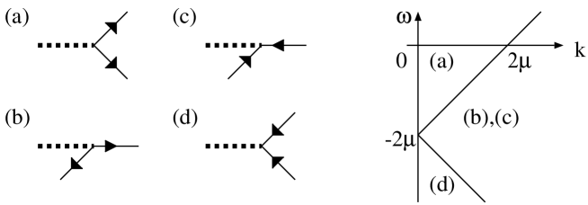
Figure 3: The left panel shows the kinetic processes contained in ${\rm Im}Q^{R}(\mbox{{\boldmath$k$}},\omega)$; the corresponding inverse processes are not shown. The dashed line denotes the diquark pair field and the solid line the quark or the antiquark. The right panel represents the energy-momentum regions in which the decay processes (a)-(d) (and their inverse ones) occur.

Here, we would like to discuss the critical behavior of the response function Eq. (25). In general, when the temperature approaches $T_{c}$ of the second-order transition from above, the fluctuations of the order parameter with a low frequency (small $\omega$) and a long wave-length (small $k$) become easily excited. This implies, on account of Eq. (15), that $D^{R}(\mbox{{\boldmath$k$}},\omega)$ with small $\omega$ and $k$ becomes larger as the system approaches the critical point. At $T_{c}$, the system becomes unstable with respect to uniform diquark-pair formation, and a finite and permanent pair-field is formed with an infinitesimally-small external field. Then, according to Eq.(15), $D^{R}({\bf 0},0)$ should be divergent at $T=T_{c}$. One can show that this is indeed the case, that is

$${D^{R}({\bf 0},0)}^{-1}\Big{|}_{T=T_{c}}=0.$$ (29)

In fact, the denominator of Eq. (25) for vanishing $k$ and $\omega$ becomes

$$1+G_{C}Q^{R}({\bf 0},0)$$

$$= 1-8G_{C}\int\frac{d^{3}\mbox{{\boldmath$p$}}}{(2\pi)^{3}}\left\{\frac{1}{p-\mu}\tanh\frac{\beta(p-\mu)}{2}+\frac{1}{p+\mu}\tanh\frac{\beta(p+\mu)}{2}\right\},$$

which is found to vanish at $T=T_{c}$, on account of Eq. (9). Equation (29) is called the Thouless criterion[51], which may be used to determine the critical point.

For the momentum integration of Eq. (27), we employ the following cutoff scheme[52, 53]. First, we note that the imaginary part of $Q^{R}(\mbox{{\boldmath$k$}},\omega)$ is free from an ultraviolet divergence. Thus, we can evaluate the imaginary part without introducing a cutoff. In this scheme, the imaginary part, Eq. (28), can be reduced to a compact form (see Appendix A),

$${\rm Im}~{}Q^{R}(\mbox{{\boldmath$k$}},\omega) = -N_{f}(N_{c}-1)T\frac{(\omega+2\mu)^{2}-k^{2}}{2\pi k}$$ (31)

$$\times\left[\log\frac{\cosh(\omega+k)/4T}{\cosh(\omega-k)/4T}-\theta(-|\omega+2\mu|+k)\frac{\omega}{2T}\right].$$

Then, we evaluate the real part of $Q^{R}(\mbox{{\boldmath$k$}},\omega)$ from the imaginary part by using the dispersion relation. We introduce a cutoff at this stage, because ${\rm Re}~{}Q^{R}(\mbox{{\boldmath$k$}},\omega)$ has an ultraviolet divergence. The cutoff should be chosen so as to satisfy the Thouless criterion for $k=0$, discussed above. Thus, as shown in Appendix A, the real part of $Q^{R}$ is expressed as

$${\rm Re}Q^{R}(\mbox{{\boldmath$k$}},\omega)=-\frac{1}{\pi}{\rm P}\int^{2\Lambda-2\mu}_{-2\Lambda-2\mu}d\omega^{\prime}\frac{{\rm Im}Q^{R}(\mbox{{\boldmath$k$}},\omega^{\prime})}{\omega-\omega^{\prime}},$$ (32)

where P denotes the principal value. This cutoff scheme has the advantages that the imaginary part of $Q^{R}(\mbox{{\boldmath$k$}},\omega)$ does not destroy any conservation laws through the introduction of a cutoff and it does reflects the symmetries of the system. In addition, the simple form Eq. (31), which is derived without introducing a cutoff, is quite convenient for numerical calculations.

3.2 Collective excitation

In this subsection, we obtain the dispersion relation of the collective mode in the diquark channel by solving Eq. (26) for $\omega$, with $k$ given. Solutions of Eq. (26) should exist in the lower-half complex energy plane $\mathbb{C}^{-}$, because the imaginary part of the pole should be negative; otherwise the system would be unstable with respect of the creation of collective modes. Thus we actually solve the equation,

$$1+G_{C}Q^{R}(\mbox{{\boldmath$k$}},z)=0$$ (33)

for a complex variable $\omega\equiv z$ with $Q^{R}(\mbox{{\boldmath$k$}},z)\equiv Q^{R}(\mbox{{\boldmath$k$}},\omega)|_{\omega\to z}$. In fact, it can be numerically verified that Eq. (33) does not have any solution in the upper-half plane $\mathbb{C}^{+}$. In order to calculate Eq. (33) for $z\in\mathbb{C}^{-}$, we must perform the analytic continuation of $Q^{R}(\mbox{{\boldmath$k$}},\omega)$ to $\mathbb{C}^{-}$; a simple analytic continuation of Eq. (24), defined as

$$Q(\mbox{{\boldmath$k$}},z)\equiv{\cal Q}(\mbox{{\boldmath$k$}},\nu_{n})|_{i\nu_{n}\to z},\qquad z\in\mathbb{C},$$ (34)

with $\mathbb{C}$ denoting the entire complex plane, has a cut along the real axis. Hence $Q^{R}(\mbox{{\boldmath$k$}},z)\neq Q(\mbox{{\boldmath$k$}},z)$ in $\mathbb{C}^{-}$. The retarded function $Q^{R}(\mbox{{\boldmath$k$}},z)$ in $\mathbb{C^{-}}$ is defined on another Riemann sheet of $Q(\mbox{{\boldmath$k$}},z)$, and therefore one has to derive the analytic function of $Q(\mbox{{\boldmath$k$}},z)$ in this Riemann sheet to solve Eq. (33). As shown in Appendix B, the form of $Q^{R}(\mbox{{\boldmath$k$}},z)$ in $\mathbb{C}^{-}$ is found to be

$$Q^{R}(\mbox{{\boldmath$k$}},z)=Q(\mbox{{\boldmath$k$}},z)+2iI(\mbox{{\boldmath$k$}},z),$$ (35)

with $I(\mbox{{\boldmath$k$}},z)\equiv\mbox{Im}Q^{R}(\mbox{{\boldmath$k$}},\omega)|_{\omega\to z}$.

Using Eq. (35), we find a solution of Eq. (33) in $\mathbb{C}^{-}$. Note that the Thouless criterion Eq.(LABEL:eqn:Thouless) ensures that there exists a solution at the origin for $T=T_{c}$, irrespective of $\mu$. The temperature dependence of the solutions with $k=0$ is already presented in Ref. ref:KKKN1. We display them in Fig. 4 for three chemical potentials, $\mu=350$, $400$ and $500$ MeV; the three curves correspond to these three values of $\mu$, while the dots on the curves denote the position of the poles for each reduced temperature, $\varepsilon\equiv(T-T_{c})/T_{c}=0,0.1,0.2,\cdots$. It can be seen that the pole goes up to the origin in the complex energy plane as $T$ is lowered toward $T_{c}$. It is also seen that the rate at which the origin is approached is almost the same for all the chemical potentials. The result clearly shows that the collective mode of the pair fluctuations is the soft mode[37] of CSC phase transition, which gives rise to the precursory phenomena of CSC phase transition, as shown in the following sections. We will see that the softening of the pole causes a rapid growth of the peak in $\rho(\mbox{{\boldmath$k$}},\omega)$ and $S(\mbox{{\boldmath$k$}},\omega)$ as $T\to T_{c}$.

Figure 4: The pole $\omega_{s}$ of the collective mode above $T_{c}$ for vanishing momentum with various $\mu$. The points denote the positions of the poles at the reduced temperature $\varepsilon\equiv(T-T_{c})/T_{c}=0$, $0.1$, $0.2\cdots$. Note here that $\omega_{s}(k=0)|_{\varepsilon=0}=0$. The pole approaches the origin as $\varepsilon$ is lowered.

It is noteworthy that ${\rm Re}~{}\omega$ is small but finite. In the weak coupling limit, as described by BCS theory, the pole of the soft mode appears on the imaginary axis, i.e., ${\rm Re}~{}\omega=0$. This is due to a particle-hole symmetry inherent in the weak coupling limit: In metal superconductors, an attractive interaction exists only for fermions with energies satisfying $|\omega|<\omega_{D}$, as measured from the Fermi energy $E_{F}$ with the Debye frequency $\omega_{D}$, which satisfies $\omega_{D}\ll E_{F}$. Thus, the DOS for the fermions participating in the pairing can be treated as a constant in this energy range, and accordingly the range is symmetric with respect to the Fermi surface. For CSC, the pairing involves all of the states in the Fermi sphere, not just those around the Fermi surface. This leads to an asymmetry between particles and holes. This asymmetry is the origin of the finite real part of the soft mode. From Fig. 4, we find that the ratio ${\rm Re}~{}\omega/{\rm Im}~{}\omega$ becomes smaller for larger $\mu$. This is plausible, because the rate of the particle-hole asymmetry becomes smaller as $\mu$ is increased. It is instructive to note that an increase of ${\rm Im}~{}\omega$, along with that of $\mu$, is also understood in a different way: The density of states on the Fermi surface into which the collective mode decays increases with the chemical potential. Thus, a larger decay probability of the collective mode is realized, and this leads to a larger ${\rm Im}~{}\omega$.

The fact that the pole has both real and imaginary parts implies that the dynamical behavior of the order parameter near $T_{c}$ is a damped-oscillator mode, while the pure imaginary poles in the weak coupling limit correspond to over-damped modes, or diffusive modes as mentioned above. However, the absolute value of ${\rm Im}~{}\omega$ is larger than that of ${\rm Re}~{}\omega$ even in the present case. This implies that the dynamical behavior of the order parameter of CSC is approximately the same as that of the over-damped case, and it is accurately described by a non-linear diffusion equation like the time-dependent Ginzburg-Landau (TDGL) equation in the weak coupling theory[54, 8].

Next, let us consider the momentum dependence of the pole $\omega_{s}(k)$. In Fig. 5, we plot ${\rm Im}\omega_{s}(k)$ as a function of $k$. It is seen that $\left|{\rm Im}\omega_{s}(k)\right|$ becomes larger as $k$ is increased. This means that the lifetime of the fluctuations of the pair field becomes shorter with smaller wavelength. The pole $\omega_{s}(k)$ in the complex energy plane is shown in the right panel of Fig. 5. It can be seen that the ratio ${\rm Re}\omega/{\rm Im}\omega$ is almost independent of $k$ and $\varepsilon$.

Figure 5: Momentum dependence of the pole $\omega_{s}(k)$ for $\mu=400$ MeV and $\varepsilon=0$, $0.2$ and $0.4$. The left panel depicts the $k$ dependence of Im$\omega_{s}(k)$. The right panel depicts the momentum dependence of $\omega_{s}(k)$ in the complex energy plane. The pole moves away from the origin as $k$ is increased.

3.3 Softening of the pair fluctuations

Figure 6: The spectral function $\rho(\mbox{{\boldmath$k$}},\omega)$ with $k=0$ for $\mu=350,400$ and $500$ MeV and several values of $\varepsilon$. The height of the peak increases as $T$ is lowered in the normal phase for all values of $\mu$. A clear peak is seen even at as high a temperature as $\varepsilon=0.2$.

In the previous subsection, we saw that quark matter at values of $T$ above but near $T_{c}$ develops a collective mode owing to diquark-pair fluctuations. In this subsection, we show how the strength of the fluctuations changes when $T$ is lowered toward $T_{c}$.

We first show the temperature dependence of $\rho(\mbox{{\boldmath$k$}},\omega)$ at vanishing momentum $\mbox{{\boldmath$k$}}=\bf 0$ for three different chemical potentials, $\mu=350,400,500$ MeV, and at several reduced temperatures in Fig. 6[8]. One can see that the position of the peak moves toward the origin, while the peak height increases as the temperature is lowered toward $T_{c}$, although the rate of growth of the peak decreases as $\mu$ is increased.

Using the Thouless criterion Eq. (LABEL:eqn:Thouless), it can be analytically shown that the spectral function has a divergent peak at the origin, $(\mbox{{\boldmath$k$}},\omega)=({\bf 0},0)$, for $T=T_{c}$. It can be seen in Fig. 6 that the peak remains quite distinct as away from $T_{c}$ as $\varepsilon=0.2$. In the case of electric superconductivity in metals, the effect of fluctuations is small, because of weak coupling. Precursory phenomena in electric conductivity can be observed experimentally. For example, there appears anomalous enhancement called ‘paraconductivity’ in the electric conductivity just above the critical temperature. However, the range of $T$ over which clear paraconductivity is seen is limited to those satisfying $\varepsilon\lesssim 10^{-3}$, even in superconductors with large fluctuations such as dirty alloys and low-dimensional materials. Therefore, we can conclude that fluctuations in CSC survive for values of $\varepsilon$ in two or three orders larger than in the case of electric superconductors. It follows that the precursory fluctuation phenomena of CSC can exist over a rather wide range of $T$, and hence they can be used as experimental signatures of CSC.

(a)                                                       (b)

Figure 7: The spectral function $\rho(\mbox{{\boldmath$k$}},\omega)$ and the dynamical structure factor $S(\mbox{{\boldmath$k$}},\omega)$ for $k=0$ at $\mu=400$ MeV.

The above arguments are based on the behavior of the spectral function $\rho(\mbox{{\boldmath$k$}},\omega)$. We can draw further conclusions on the strength of the fluctuations if we consider the dynamical structure factor $S(\mbox{{\boldmath$k$}},\omega)$, defined in Eq. (20). As mentioned above, $S(\mbox{{\boldmath$k$}},\omega)$ is more directly related to observables than the spectral function $\rho(\mbox{{\boldmath$k$}},\omega)$, which has a negative value for bosons when $\omega<0$, as shown in Fig. 7. We display the $\varepsilon$ dependence of $S(\mbox{{\boldmath$k$}},\omega)$ for $\mu=400$ MeV at vanishing momentum transfer in Fig. 7 (b). It can be seen that a peak appears in $S(\mbox{{\boldmath$k$}},\omega)$ and moves toward the origin as the temperature approaches $T_{c}$. This behavior is consistent with that of the spectral function, and it is a reflection of the softening of the pair fluctuations. We remark that the position of the pole corresponds to the peak of the dynamical structure factor, not the spectral function.

Next, we show the energy-momentum dependence of $S(\mbox{{\boldmath$k$}},\omega)$ at $\mu=400$ MeV and $\varepsilon=0.02$ and $0.1$ in Fig. 8. The peak near $\omega=0$ flattens as $k$ is increased in each figure, which means that the fluctuations with smaller wavelength tend to be suppressed.

Figure 8: The energy and momentum dependence of $S(\mbox{{\boldmath$k$}},\omega)$ for $\mu=400$ MeV. Here, we have $\varepsilon=0.02$ ($\varepsilon=0.1$) in the left (right) panel. The peak in $S(\mbox{{\boldmath$k$}},\omega)$ grows, which implies that the pair fluctuations around $\omega=k=0$ become stronger, as $\varepsilon$ approaches $0$.

4 Specific heat

In the previous section, we showed that there exist strong pair fluctuations even well above $T_{c}$. In the present and following sections, we evaluate the effects of the pair fluctuations on some observables. In this section, we calculate the specific heat, taking into account the precursory fluctuations above $T_{c}$, and show that the pair fluctuations cause an anomalous enhancement of the specific heat over range of $T$ that is similar to that over which a prominent peak in the spectral function is seen.

The specific heat per unit volume, $c_{\rm v}$, is calculated from the thermodynamic potential per unit volume, $\Omega$, as

$$c_{\rm v}=-T\frac{\partial^{2}\Omega}{\partial T^{2}}.$$ (36)

Therefore, we first evaluate the thermodynamic potential $\Omega$ in the normal phase, incorporating the pair fluctuations:

$$\Omega=\Omega_{0}+\Omega_{\rm fl.}.$$ (37)

Here, $\Omega_{0}$ ($\Omega_{\rm fl.}$) denotes the contribution at the mean-field level (from the pair fluctuations). Then, the specific heat $c_{\rm v}$ is also divided into the two parts, corresponding to $\Omega_{0}$ and $\Omega_{\rm fl.}$, respectively:

$$c_{\rm v}=c_{\rm v}^{0}+c_{\rm v}^{\rm fl.}.$$ (38)

Figure 9: The diagrams taken into account in the calculation of the thermodynamic potential $\Omega=\Omega_{0}+\Omega_{\rm fl.}$. Here, $\Omega_{0}$ is the thermodynamic potential of a free fermionic system, and $\Omega_{\rm fl.}$ is the contribution from the fluctuations of the pair field.

The thermodynamic potential of the free quarks $\Omega_{0}$ reads

$$\Omega_{0} = \Omega_{MF}(M=0,\Delta=0)$$ (39)

$$= T\sum_{n}\int\frac{d^{3}\mbox{{\boldmath$k$}}}{(2\pi)^{3}}{\rm Tr}\log{\cal G}_{0}(\mbox{{\boldmath$k$}},\nu_{n}).$$

Here, $\Omega_{\rm fl.}$ consists of the summation of the ring diagrams shown in Fig. 9, where all vertices correspond to the diquark interaction term Eq. (2). Below, we find that these diagrams correspond to those considered in the response function $D^{R}(\mbox{{\boldmath$k$}},\omega)$ in the RPA, and hence $\Omega_{\rm fl.}$ exhibits anomalous behavior through $D^{R}(\mbox{{\boldmath$k$}},\omega)$. The lowest-order diagram in $\Omega_{\rm fl.}$ is calculated to be

$$\Omega_{\rm fl.}^{(1)} = -2G_{C}T^{2}\sum_{m,n}\int\frac{d^{3}\mbox{{\boldmath$p$}}_{1}d^{2}\mbox{{\boldmath$p$}}_{2}}{(2\pi)^{6}}\sum_{A=2,5,7}\mbox{Tr}\left[i\gamma_{5}\tau_{2}\lambda_{A}{\cal G}(\mbox{{\boldmath$p$}}_{1},\omega_{m})i\gamma_{5}\tau_{2}\lambda_{A}{\cal G}(\mbox{{\boldmath$p$}}_{2},\omega_{n})\right]$$ (40)

$$= -2G_{C}T^{2}\sum_{m,n}\int\frac{d^{3}\mbox{{\boldmath$p$}}_{1}d^{2}\mbox{{\boldmath$p$}}_{2}}{(2\pi)^{6}}3\mbox{Tr}\left[i\gamma_{5}\tau_{2}\lambda_{2}{\cal G}(\mbox{{\boldmath$p$}}_{1},\omega_{m})i\gamma_{5}\tau_{2}\lambda_{2}{\cal G}(\mbox{{\boldmath$p$}}_{2},\omega_{n})\right]$$

$$= 3T\sum_{n}\int\frac{d^{3}\mbox{{\boldmath$p$}}}{(2\pi)^{3}}G_{C}{\cal Q}(\mbox{{\boldmath$p$}},\nu_{n}).$$

In the second equality here, we have used the fact that the $A=2,5$ and 7 terms in the first line of Eq. (40) give the same contribution; we have incorporated them all into the $A=2$ term with an overall factor of $3$. Physically, this factor corresponds to the existence of three degenerate collective excitations of the pair field in the normal phase, that is, the red-blue, blue-green and green-red collective modes in the color space. This factor appears in the diagrams of $\Omega_{\rm fl.}$ at all orders. Similarly, the $l$-th order diagrams of $\Omega_{\rm fl.}$ can be evaluated as

$$\Omega_{\rm fl.}^{(l)}=-\frac{3}{l}T\sum_{n}\int\frac{d^{3}\mbox{{\boldmath$p$}}}{(2\pi)^{3}}\left[-G_{C}{\cal Q}(\mbox{{\boldmath$p$}},\nu_{n})\right]^{l}.$$ (41)

Summing up all the terms, we obtain

$$\Omega_{\rm fl.}=\sum_{l=1}^{\infty}\Omega_{\rm fl.}^{(l)} = -3T\sum_{n}\int\frac{d^{3}\mbox{{\boldmath$p$}}}{(2\pi)^{3}}\sum_{l=1}^{\infty}\frac{1}{l}\left[-G_{C}{\cal Q}(\mbox{{\boldmath$p$}},\nu_{n})\right]^{l}$$

$$= 3T\sum_{n}\int\frac{d^{3}\mbox{{\boldmath$p$}}}{(2\pi)^{3}}\log\left[1+G_{C}{\cal Q}(\mbox{{\boldmath$p$}},\nu_{n})\right]$$

$$= 3\int\frac{d^{3}\mbox{{\boldmath$p$}}}{(2\pi)^{3}}\int_{C}\frac{dz}{2\pi i}\frac{1}{{\rm e}^{\beta z}-1}\log\left[1+G_{C}Q(\mbox{{\boldmath$p$}},z)\right]$$

$$= \frac{3}{\pi}\int\frac{d^{3}\mbox{{\boldmath$p$}}}{(2\pi)^{3}}{\rm P}\int d\omega\frac{1}{{\rm e}^{\beta\omega}-1}\mbox{Im}\log\left[1+G_{C}Q^{R}(\mbox{{\boldmath$p$}},\omega)\right].$$ (43)

In the last equality, the contour of integration is modified so as to avoid the cut along the real axis, as shown in Fig. 10[55]. Note that the argument of the logarithmic function is the same as the denominator of the response function of the pair field $D^{R}(\mbox{{\boldmath$k$}},\omega)$, which, we have seen, exhibits a singular behavior near $T_{c}$. Therefore, $\Omega_{\rm fl.}$ should also show an anomalous behavior near $T_{c}$, which gives rise to an enhancement of $c_{\rm v}^{\rm fl.}$ [51].

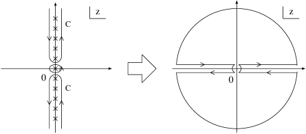
Figure 10: The contour of integration in Eq. (43).

Before taking the derivatives in Eq. (36), we expand the argument of the logarithmic function in Eq. (43) in a Taylor expansion about $\omega=k=0$ and $T=T_{c}$. To lowest order, this yields

$$G_{C}^{-1}+Q^{R}(\mbox{{\boldmath$k$}},\omega)\simeq C_{0}\omega+C|\mbox{{\boldmath$k$}}|^{2}+A\varepsilon,$$ (44)

with

$$C_{0}=\left.\frac{\partial Q^{R}({\bf 0},0)}{\partial\omega}\right|_{T=T_{c}},\,C=\left.\frac{\partial Q^{R}({\bf 0},0)}{\partial|{\bf k}|^{2}}\right|_{T=T_{c}},\,A=\left.T\frac{\partial Q^{R}({\bf 0},0)}{\partial T}\right|_{T=T_{c}}.$$ (45)

Note that there is no zeroth-order term in the expansion Eq. (44). This follows from the Thouless criterion, $G_{C}^{-1}+Q^{R}({\bf 0},0)|_{T=T_{c}}=0$. One can numerically check that the right-hand side of Eq. (44) indeed does provide a good approximation of the behavior of the left hand side over a rather wide region of $\omega$, $k$ and $\varepsilon$; roughly for those values satisfying $|\omega|,|\mbox{{\boldmath$k$}}|\lesssim 120$ MeV and $\varepsilon\lesssim 0.3$[56]. As was shown in the previous section, the strength of the pair field is concentrated around $\omega=|\mbox{{\boldmath$k$}}|=0$ as $T$ approaches $T_{c}$. Therefore, the fluctuating modes in the vicinity of the origin of the $\omega$-$k$ plane are expected to give the dominant contribution to the thermodynamic potential and hence the specific heat. Thus, use of the simple expansion given in Eq. (44) in their calculation is justified.

Figure 11: The specific heat per unit volume in the free fermionic system, $c_{\rm v}^{0}$, and the effects of the fluctuations of the pair field, $c_{\rm v}^{\rm fl.}$. The total specific heat of the system is $c_{\rm v}=c_{\rm v}^{0}+c_{\rm v}^{\rm fl.}$. It is seen that as $\varepsilon$ decreases, the enhancement of $c_{\rm v}^{\rm fl.}$ begins to become appreciable near $\varepsilon=0.05$-$0.1$. The dot-dashed curve represents the specific heat obtained with only the static part of $\Omega_{\rm fl.}$.

In Fig. 11, we plot the behavior of the specific heat $c_{\rm v}^{0}$ and $c_{\rm v}^{\rm fl.}$, above $T_{c}$. It is seen that $c_{\rm v}^{\rm fl.}$ diverges as $T\to T_{c}$. A clear enhancement of $c_{\rm v}^{\rm fl.}$ is seen already near $\varepsilon=0.05$-$0.1$. The range of temperatures in which $c_{\rm v}^{\rm fl.}$ is larger than $c_{\rm v}^{0}$ is called the Ginzburg-Levanyuk region[57, 58]. In our case, the Ginzburg-Levanyuk region exists up to $\varepsilon=0.02$ above $T_{c}$. In electric superconductors, the Ginzburg-Levanyuk region is continued only to values $\varepsilon$ satisfying $\varepsilon\lesssim 10^{-3}$, even for dirty alloys. Therefore, the Ginzburg-Levanyuk region for CSC is very much larger than that for electric superconductors. It can be numerically checked that $c_{\rm v}^{\rm fl.}\sim\varepsilon^{-1/2}$ near $T_{c}$. This critical exponent of $c_{\rm v}$ is the same as that obtained from the Ginzburg-Landau equation without nonlinear terms[59]. This is because we have adopted the RPA for the pair field. However, the RPA is not valid in the vicinity of $T_{c}$, because there the amplitude of the fluctuations becomes large, and therefore the nonlinear effects begin to play a significant role. For this reason, the true critical exponent of the specific heat should differ from $-1/2$.

The singular behavior of the specific heat above $T_{c}$ of the superconductivity is usually studied using only the static part of $\Omega_{\rm fl.}$[59], i.e., the $n=0$ component of the Matsubara sum in Eq. (4). However, we have explicitly included the dynamical modes as well. We now give an account of the relation between the two approaches. The most singular behavior of $\Omega_{\rm fl.}$ which causes the enhancement of $c_{\rm v}^{\rm fl.}$ near $T_{c}$ certainly comes from the static part of $\Omega_{\rm fl.}$, because only the static part in Eq. (4) diverges as $\varepsilon\to 0$. Therefore, the contribution from the static part dominates the behavior of $\Omega_{\rm fl.}$, at least near $T_{c}$. In Fig. 11, the specific heat obtained using only the static part is plotted by the dot-dashed curve. It is seen that the singular behavior of $c_{\rm v}^{\rm fl.}$ near $T_{c}$ is reproduced by the contribution from the static part of $\Omega_{\rm fl.}$ alone, and the contribution from the $n\neq 0$ components of $\Omega_{\rm fl.}$ to $c_{\rm v}^{\rm fl.}$ is smaller than $c_{\rm v}^{0}$.

Recently, Voskresensky calculated the specific heat above the CFL phase and found that the Ginzburg-Levanyuk region exists up to $\varepsilon\sim 1$[9], which is more than one order of magnitude larger in the units of $\varepsilon$ than that found in the present case. The origin of this difference can be understood as follows. In two-flavor quark matter, the degeneracy of the collective modes gives rise to the factor of $3$ in Eq. (43), while the existence of nine collective modes above $T_{c}$ for the CFL phase can cause a factor of $9$ to appear in $c_{\rm v}^{\rm fl.}$, provided that the strange quark mass is ignored. Therefore, $c_{\rm v}^{\rm fl.}$ above the CFL phase can take a value three times larger than that in ours. The coefficients of the Ginzburg-Landau equation in Ref. ref:Vosk04, which are determined in the weak coupling limit, further increase $c_{\rm v}^{\rm fl.}$. These factors can account for the wide Ginzburg-Levanyuk region obtained in Ref. ref:Vosk04.

5 Non-Fermi liquid behavior due to fluctuations

As seen in the previous sections, the pair fluctuations form a well-developed collective mode near $T_{c}$ in CSC, and they cause anomalous behavior in the specific heat. In this section, we explore how the pair fluctuations in turn affect the properties of quarks. We show that the pair fluctuations give rise to non-Fermi liquid behavior of the quarks near $T_{c}$: It is shown, for instance, that a large decay width is acquired by the quarks near the Fermi surface. It is also shown that the anomalous behavior leads to the pseudogap in the DOS of the quarks.

The pair field may exhibit both amplitude and phase fluctuations. We assume that the amplitude fluctuations dominate the phase fluctuations[29]. Thus we are led to employ the T-matrix approximation[60], which is suitable to evaluate the effects of the amplitude fluctuations of the pair field on the quarks. Historically, the DOS above $T_{c}$ was first calculated within the T-matrix approximation for the case of the electric superconductivity in the weak coupling regime more than three decades ago [61, 62, 63]. It was shown that a pseudogap can form but only in the vicinity of $T_{c}$. After the discovery of the HTSC, the same approximation was reconsidered in the strong coupling regime in the study of the DOS for HTSC[64, 30]. In this section, we compute the quark Green function in the T-matrix approximation and evaluate the spectral function and the dispersion relation of the quarks in the relativistic kinematics.

5.1 T-matrix approach

The one-particle quark spectral function is defined by

$${\cal A}(\mbox{{\boldmath$k$}},\omega) = -\frac{1}{\pi}\cdot{\rm Im}G^{R}(\mbox{{\boldmath$k$}},\omega)$$ (46)

$$= -\frac{1}{\pi}\frac{G^{R}(\mbox{{\boldmath$k$}},\omega)-G^{A}(\mbox{{\boldmath$k$}},\omega)}{2i}=-\frac{1}{\pi}\frac{G^{R}(\mbox{{\boldmath$k$}},\omega)-\gamma^{0}G^{R{\dagger}}(\mbox{{\boldmath$k$}},\omega)\gamma^{0}}{2i},$$

where $G^{R}(\mbox{{\boldmath$k$}},\omega)$ and $G^{A}(\mbox{{\boldmath$k$}},\omega)$ are the retarded and advanced Green functions of the quarks, respectively. Conversely, $G^{R}(\mbox{{\boldmath$k$}},\omega)$ is given in terms of ${\cal A}(\mbox{{\boldmath$k$}},\omega)$ as

$$G^{R}(\mbox{{\boldmath$k$}},\omega) = \int d\omega^{\prime}\frac{{\cal A}(\mbox{{\boldmath$k$}},\omega^{\prime})}{\omega-\omega^{\prime}+i\eta}.$$ (47)

The spectral function ${\cal A}(\mbox{{\boldmath$k$}},\omega)$ has a Dirac matrix structure in the relativistic formalism. From the rotational and parity invariances, the Dirac indices of ${\cal A}(\mbox{{\boldmath$k$}},\omega)$ can be decomposed into three parts,

$${\cal A}(\mbox{{\boldmath$k$}},\omega)=\rho_{0}(\mbox{{\boldmath$k$}},\omega)\gamma^{0}-\rho_{\rm v}(\mbox{{\boldmath$k$}},\omega)\hat{\mbox{{\boldmath$k$}}}\cdot{\mbox{{\boldmath$\gamma$}}}+\rho_{\rm s}(\mbox{{\boldmath$k$}},\omega),$$ (48)

with $\hat{\mbox{{\boldmath$k$}}}={\mbox{{\boldmath$k$}}}/|{\mbox{{\boldmath$k$}}}|$. Actually, $\rho_{\rm s}(\mbox{{\boldmath$k$}},\omega)$ vanishes in the chiral limit, which we have taken. Note that $\rho_{0}(\mbox{{\boldmath$k$}},\omega)$ is related to the number density of quarks, and hence to the DOS of the quarks, as

$$N(\omega) = 4\int\frac{d^{3}{\mbox{{\boldmath$k$}}}}{(2\pi)^{3}}{\rm Tr}_{\rm c,f}\left[\rho_{0}({\mbox{{\boldmath$k$}}},\omega)\right],$$ (49)

with ${\rm Tr}_{\rm c,f}$ denoting the trace over color and flavor indices.

To calculate the quark Green function Eq. (47), we use the Matsubara formalism. The Dyson-Schwinger equation for the quark Matsubara Green function ${\cal G}(\mbox{{\boldmath$k$}},\omega_{n})$ reads

$${\cal G}(\mbox{{\boldmath$k$}},\omega_{n}) = {\cal G}_{0}(\mbox{{\boldmath$k$}},\omega_{n})+{\cal G}_{0}(\mbox{{\boldmath$k$}},\omega_{n})\tilde{\Sigma}(\mbox{{\boldmath$k$}},\omega_{n}){\cal G}(\mbox{{\boldmath$k$}},\omega_{n}),$$ (50)

where $\tilde{\Sigma}(\mbox{{\boldmath$k$}},\omega_{n})$ is the quark self-energy in the imaginary-time formalism. We take the following approximate form for the self-energy $\tilde{\Sigma}(\mbox{{\boldmath$k$}},\omega_{n})$

$$\tilde{\Sigma}(\mbox{{\boldmath$p$}},\omega_{n}) = 4\sum_{A=2,5,7}(\lambda_{A})^{2}T\sum_{m}\int\frac{d^{3}\mbox{{\boldmath$k$}}}{(2\pi)^{3}}\tilde{\Xi}(\mbox{{\boldmath$p$}}+\mbox{{\boldmath$k$}},\omega_{n}+\omega^{\prime}_{m}){\cal G}_{0}(\mbox{{\boldmath$k$}},\omega^{\prime}_{m})$$ (51)

$$= 8T\sum_{m}\int\frac{d^{3}\mbox{{\boldmath$k$}}}{(2\pi)^{3}}\tilde{\Xi}(\mbox{{\boldmath$p$}}+\mbox{{\boldmath$k$}},\omega_{n}+\omega^{\prime}_{m}){\cal G}_{0}(\mbox{{\boldmath$k$}},\omega^{\prime}_{m}),$$ (52)

where the T-matrix $\tilde{\Xi}(\mbox{{\boldmath$k$}},\nu_{n})$ is

$$\tilde{\Xi}(\mbox{{\boldmath$k$}},\nu_{n})=-G_{C}\frac{1}{1+G_{C}{\cal Q}({\mbox{{\boldmath$k$}}},\nu_{n})}=-G_{C}\left(1-2G_{C}{\cal D}(\mbox{{\boldmath$k$}},\nu_{n})\right),$$ (53)

with ${\cal D}(\mbox{{\boldmath$k$}},\nu_{n})$ defined in Eq. (23). This is the so-called non-self-consistent T-matrix approximation, which is consistent with RPA employed in §3 to describe the pair fluctuations. Figure 12 is the schematic representation of our T-matrix approximation; the thin and bold lines represent the free and full Matsubara propagators, ${\cal G}_{0}(\mbox{{\boldmath$k$}},\omega)$ and ${\cal G}(\mbox{{\boldmath$k$}},\omega)$. If the thin lines in the diagram are replaced by the bold lines, the approximation becomes the self-consistent approximation. We comment on this approximation in the concluding remarks. The T-matrix $\tilde{\Xi}(\mbox{{\boldmath$k$}},\nu_{n})$ show the same anomalous behavior as the response function near $T_{c}$, in accordance with the softening of the pair fluctuations.

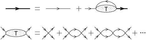
Figure 12: The Feynman diagrams representing the quark Green function in the non-self-consistent T-matrix approximation. The thin lines represent the free propagator ${\cal G}_{0}$, while the bold lines represent the full propagator ${\cal G}$.

In the second equality of Eq. (52), we have used the fact that the sum of the Gell-Mann matrices in Eq. (51) yields $\sum_{A}(\lambda_{A})^{2}=2$. This factor corresponds to the two possible patterns of $\tilde{\Sigma}(\mbox{{\boldmath$k$}},\omega_{n})$ in the color space owing to the existence of three degenerate collective modes of the pair field in the normal phase; a red quark, for example, can create a red-green and red-blue collective modes incorporating green or blue quarks, respectively. In the case of the specific heat discussed in §4, the factor $3(=N_{c})$ appears because the three degenerate collective modes contribute equally. On the other hand, only two of the three collective modes can couple to an incoming quark, and this is the reason that the factor $2(=N_{c}-1)$ arises in the self-energy appearing in Eq. (52).

The analytic continuation of $\tilde{\Sigma}(\mbox{{\boldmath$k$}},\omega_{n})$ to the real axis from the upper-half complex energy plane gives the self-energy in real time,

$$\Sigma^{R}(\mbox{{\boldmath$k$}},\omega)=\tilde{\Sigma}(\mbox{{\boldmath$k$}},\omega_{n})|_{i\omega_{n}\to\omega+i\eta}.$$ (54)

After several manipulations (summarized in Appendix C), this self-energy is found to be

$$\Sigma^{R}(\mbox{{\boldmath$p$}},\omega) = 2\int\frac{d^{4}q}{(2\pi)^{4}}\left\{\tanh\frac{q^{0}}{2T}\Xi^{R}(\mbox{{\boldmath$p$}}+\mbox{{\boldmath$q$}},\omega+q^{0}){\rm Im}G_{0}^{R}(\mbox{{\boldmath$q$}},q^{0})\right.$$ (55)

$$\left.\qquad\qquad+\coth\frac{q^{0}}{2T}{\rm Im}\Xi^{R}(\mbox{{\boldmath$p$}}+\mbox{{\boldmath$q$}},q^{0})G_{0}^{A}(\mbox{{\boldmath$q$}},q^{0}-\omega)\right\},$$

with

$$\Xi^{R}(\mbox{{\boldmath$k$}},\omega)=\tilde{\Xi}(\mbox{{\boldmath$k$}},\nu_{n})|_{i\nu_{n}=\omega+i\eta}=-[G_{C}^{-1}+Q^{R}(\mbox{{\boldmath$k$}},\omega)]^{-1}.$$ (56)

The imaginary part of Eq. (55) is

$$\mbox{Im}\Sigma^{R}(\mbox{{\boldmath$p$}},\omega)$$ (57)

$$= 2\int\frac{d^{4}q}{(2\pi)^{4}}\left(\tanh\frac{q^{0}}{2T}-\coth\frac{q^{0}+\omega}{2T}\right)\mbox{Im}\Xi^{R}(\mbox{{\boldmath$p$}}+\mbox{{\boldmath$q$}},\omega+q^{0})\mbox{Im}G^{R}(\mbox{{\boldmath$q$}},q^{0}).\qquad$$

Using Eq. (55), the retarded Green function, Eq. (47), can be written

$$G^{R}(\mbox{{\boldmath$k$}},\omega)=\frac{1}{[G_{0}^{R}(\mbox{{\boldmath$k$}},\omega)]^{-1}-\Sigma^{R}(\mbox{{\boldmath$k$}},\omega)}.$$ (58)

From the rotational and parity invariances, we find that the self-energy has the same Dirac matrix structure as the spectral function,

$$\Sigma^{R}(\mbox{{\boldmath$k$}},\omega)=\Sigma_{0}(\mbox{{\boldmath$k$}},\omega)\gamma^{0}-\Sigma_{\rm v}(\mbox{{\boldmath$k$}},\omega)\hat{\mbox{{\boldmath$k$}}}\cdot\mbox{{\boldmath$\gamma$}}+\Sigma_{\rm s}(\mbox{{\boldmath$k$}},\omega),$$ (59)

with $\Sigma_{0}=(1/4){\rm Tr}[\Sigma^{R}\gamma^{0}]$, $\Sigma_{\rm v}=(1/4){\rm Tr}[\Sigma^{R}\hat{\mbox{{\boldmath$k$}}}\cdot\mbox{{\boldmath$\gamma$}}]$ and $\Sigma_{\rm s}=(1/4){\rm Tr}[\Sigma^{R}]$. From Eq. (55), one can easily check that $\Sigma_{\rm s}$ vanishes in the chiral limit, which also means that $\rho_{\rm s}=0$ in this case.

It is useful to decompose $\Sigma^{R}(\mbox{{\boldmath$k$}},\omega)$ and ${\cal A}(\mbox{{\boldmath$k$}},\omega)$ into positive and negative energy parts using the projection operators $\Lambda_{\mp}(\mbox{{\boldmath$k$}})=(1\pm\gamma^{0}\mbox{{\boldmath$\gamma$}}\cdot\hat{\mbox{{\boldmath$k$}}})/2$. We obtain

$$\Sigma^{R}(\mbox{{\boldmath$k$}},\omega) = \gamma^{0}(\Sigma_{-}(\mbox{{\boldmath$k$}},\omega)\Lambda_{-}(\mbox{{\boldmath$k$}})+\Sigma_{+}(\mbox{{\boldmath$k$}},\omega)\Lambda_{+}(\mbox{{\boldmath$k$}})),$$

$${\cal A}(\mbox{{\boldmath$k$}},\omega) = (\rho_{-}(\mbox{{\boldmath$k$}},\omega)\Lambda_{-}(\mbox{{\boldmath$k$}})+\rho_{+}(\mbox{{\boldmath$k$}},\omega)\Lambda_{+}(\mbox{{\boldmath$k$}}))\gamma^{0},$$ (60)

where

$$\Sigma_{\mp}(\mbox{{\boldmath$k$}},\omega) = \frac{1}{2}{\rm Tr}[\Sigma^{R}(\mbox{{\boldmath$k$}},\omega)\Lambda_{\mp}(\mbox{{\boldmath$k$}})\gamma^{0}]=\Sigma_{0}(\mbox{{\boldmath$k$}},\omega)\mp\Sigma_{\rm v}(\mbox{{\boldmath$k$}},\omega),$$ (61)

$$\rho_{\mp}(\mbox{{\boldmath$k$}},\omega) = \frac{1}{2}{\rm Tr}[{\cal A}(\mbox{{\boldmath$k$}},\omega)\gamma^{0}\Lambda_{\mp}(\mbox{{\boldmath$k$}})]=\frac{1}{\pi}{\rm Im}\frac{1}{\omega+\mu\mp k-\Sigma_{\mp}(\mbox{{\boldmath$k$}},\omega)}$$ (62)

$$= \rho_{0}(\mbox{{\boldmath$k$}},\omega)\pm\rho_{\rm v}(\mbox{{\boldmath$k$}},\omega)$$

are the self-energies and spectral functions for positive and negative energies, respectively. Using Eq. (61), the retarded Green function is written as

$$G^{R}(\mbox{{\boldmath$k$}},\omega) = \frac{\Lambda_{-}(\mbox{{\boldmath$k$}})\gamma^{0}}{\omega+\mu-k-\Sigma^{-}(\mbox{{\boldmath$k$}},\omega)+i\eta}+\frac{\Lambda_{+}(\mbox{{\boldmath$k$}})\gamma^{0}}{\omega+\mu+k-\Sigma^{+}(\mbox{{\boldmath$k$}},\omega)+i\eta}$$ (63)

$$= \frac{\Lambda_{-}(\mbox{{\boldmath$k$}})\gamma^{0}}{R_{-}(\mbox{{\boldmath$k$}},\omega)+i\eta}+\frac{\Lambda_{+}(\mbox{{\boldmath$k$}})\gamma^{0}}{R_{+}(\mbox{{\boldmath$k$}},\omega)+i\eta}.$$ (64)

In the second equality, we have defined

$$R_{\mp}(\mbox{{\boldmath$k$}},\omega)\equiv\omega+\mu\mp k-\Sigma_{\mp}(\mbox{{\boldmath$k$}},\omega),$$ (65)

for later convenience. The equations

$${\rm Re}~{}R_{\mp}(\mbox{{\boldmath$k$}},\omega_{\mp})=0,$$ (66)

give the dispersion relations for quarks and anti-quarks $\omega=\omega_{\mp}(\mbox{{\boldmath$k$}})$, respectively.

There are several possible choices of the four-momentum cutoff for the integral in Eq. (55). To compute this integral, we first calculate the imaginary part Eq. (57); substituting the explicit formula for ${\rm Im}~{}G_{0}^{R}(\mbox{{\boldmath$k$}},\omega)$ to Eq. (57), the $q^{0}$ integral is removed by the delta function in ${\rm Im}~{}G_{0}^{R}(\mbox{{\boldmath$k$}},\omega)$ (see, Eqs. (103) and (LABEL:eqn:ImSigV)). Then, ${\rm Im}~{}\Sigma^{R}(\mbox{{\boldmath$k$}},\omega)$ is calculated using the usual three-momentum cutoff $\Lambda$. The real part is then evaluated from ${\rm Im}~{}\Sigma^{R}(\mbox{{\boldmath$k$}},\omega)$ through the dispersion relation. To calculate ${\rm Re}~{}\Sigma^{R}(\mbox{{\boldmath$k$}},\omega)$ with the dispersion relation, we again need to introduce a cutoff. Here, we assume that the cutoff for the dispersion relation is the same as the momentum cutoff $\Lambda$, and we then have

$$\mbox{Re}\Sigma^{R}(\mbox{{\boldmath$k$}},\omega)=-\frac{1}{\pi}{\rm P}\int_{-\Lambda}^{\Lambda}d\omega^{\prime}\frac{\mbox{Im}\Sigma^{R}(\mbox{{\boldmath$k$}},\omega^{\prime})}{\omega-\omega^{\prime}}.$$ (67)

We have checked numerically that the quark spectral function and the DOS near the Fermi energy are hardly affected by the choice of the cutoff in Eq. (67).

5.2 The quasiparticle picture of quarks

Now we present the numerical results and discuss the properties of the quarks above $T_{c}$. To investigate the quasiparticle picture of the quarks, it is useful to consider the behavior of the dispersion relation $\omega=\omega_{\mp}(\mbox{{\boldmath$k$}})$ and the spectral function $\rho_{0}(\mbox{{\boldmath$k$}},\omega)$. Here, $\omega_{\mp}(\mbox{{\boldmath$k$}})$ is defined above; see Eq.(66). A remark is in order here. Because $\omega_{\mp}(\mbox{{\boldmath$k$}})$ is only the solution to the real part but not the whole part of $R_{\mp}(\mbox{{\boldmath$k$}},\omega_{\mp})$, $\omega_{\mp}(\mbox{{\boldmath$k$}})$ may not correspond to the peak position of the spectral function and does not represent physical excitations when the imaginary part of the Green function is large.

We plot the the dispersion relation of the positive energy quarks $\omega=\omega_{-}(\mbox{{\boldmath$k$}})$ for $\mu=400$ MeV and $\varepsilon=0.01$ in the left panel of Fig. 13. One sees from the figure that the dispersion relation deviates from that for free quarks, $\omega=k-\mu$, (dotted line) and exhibits a rapid increase around the Fermi energy, $\omega=0$. We also show $(\partial\omega(\mbox{{\boldmath$k$}})/\partial|\mbox{{\boldmath$k$}}|)^{-1}$ in the right panel of Fig. 13. This quantity is proportional to the DOS, provided that the imaginary part of the self-energy is ignored. As shown in the figure, there appears a pronounced minimum of $(\partial\omega(\mbox{{\boldmath$k$}})/\partial|\mbox{{\boldmath$k$}}|)^{-1}$ near the Fermi momentum, $k_{F}=\mu$, reflecting the rapid increase of $\omega_{-}(\mbox{{\boldmath$k$}})$. Although this rapid increase may not be physical because there exists a large imaginary part of the self-energy in this kinematical region, it may suggest that the gap-like structure is induced in the dispersion relation as a precursor to CSC. We will see that this is the case from the behavior of the spectral function.

Figure 13: The dispersion relation for the quarks, $\omega=\omega_{-}(\mbox{{\boldmath$k$}})$ in the left panel, and $(\partial\omega(\mbox{{\boldmath$k$}})/\partial|\mbox{{\boldmath$k$}}|)^{-1}$ in the right panel with $\mu=400$ MeV and $\varepsilon\equiv(T-T_{c})/T_{c}=0.01$. Near the Fermi momentum $k_{F}=\mu$, we see a rapid increase of $\omega_{-}(\mbox{{\boldmath$k$}})$ and a pronounced minimum of $(\partial\omega(\mbox{{\boldmath$k$}})/\partial|\mbox{{\boldmath$k$}}|)^{-1}$ around $k=k_{F}$, which means that a gap-like structure is induced in the dispersion relation as a precursor to CSC.

We show the spectral function $\rho_{0}(\mbox{{\boldmath$k$}},\omega)$ for $\mu=400$ MeV with $\varepsilon=0.01$ and $0.2$ in Fig. 14. One can see two families of peaks in both figures, near $\omega=k-\mu$ and $\omega=-k-\mu$, which correspond to the quasiparticle peaks of the quarks and anti-quarks, respectively. A notable point is that the quasiparticle peak has a clear depression around the Fermi energy, $\omega=0$, which represents the enhancement of the decay rate of the quasiparticles around the Fermi energy. Thus the depression becomes more pronounced as $\varepsilon$ becomes smaller. This behavior is quite different from that of the conventional Fermi liquids, for which the lifetime of the quasiparticles becomes longer as $\omega$ approaches the Fermi energy, $\omega=0$.

Figure 14: The spectral function $\rho_{0}$ at $\mu=400$ MeV and $\varepsilon=0.01$ and $0.2$. The peaks near $\omega=k-\mu$ and $\omega=-k-\mu$ correspond to the quark and anti-quark quasiparticles, respectively. Note that there is a depression around $\omega=0$, which is responsible for the pseudogap formation.

To understand these types of non-Fermi liquid behavior of $\omega_{-}(\mbox{{\boldmath$k$}})$ and $\rho_{0}(\mbox{{\boldmath$k$}},\omega)$ near $\omega=0$, we investigate the quark self-energy $\Sigma^{R}(\mbox{{\boldmath$k$}},\omega)$. Before giving the numerical results, we note that the spectral function of the negative energy $\rho_{+}(\mbox{{\boldmath$k$}},\omega)$ always takes small values around $\omega=0$, because the real part of $R_{+}(\mbox{{\boldmath$k$}},\omega)$, ${\rm Re}~{}R_{+}(\mbox{{\boldmath$k$}},\omega)\simeq\omega+\mu+k$, does not become smaller around $\omega=0$. Thus, $\rho_{0}(\mbox{{\boldmath$k$}},\omega)$ near the Fermi energy is reproduced by $\rho_{-}(\mbox{{\boldmath$k$}},\omega)$ alone:

$$\rho_{0}(\mbox{{\boldmath$k$}},\omega)=\frac{\rho_{-}(\mbox{{\boldmath$k$}},\omega)+\rho_{+}(\mbox{{\boldmath$k$}},\omega)}{2}\simeq\frac{1}{2}\rho_{-}(\mbox{{\boldmath$k$}},\omega).$$ (68)

Therefore, it is sufficient to consider the self-energy of the positive energy $\Sigma_{-}(\mbox{{\boldmath$k$}},\omega)$ in order to understand the non-Fermi liquid behavior of $\omega_{-}(\mbox{{\boldmath$k$}})$ and $\rho_{0}(\mbox{{\boldmath$k$}},\omega)$.

Figure 15: The self-energy $\Sigma_{-}$ for $k=k_{F}$ with $\mu=400$ MeV and $\varepsilon=0.01$. We observe a peak in Im$\Sigma_{-}$ and a rapid increase of Re$\Sigma_{-}$ at the same $\omega=0$.

In Fig. 15, we plot the real and imaginary parts of $\Sigma_{-}(\mbox{{\boldmath$k$}},\omega)|_{k=k_{F}}$ for $\mu=400$ MeV and $\varepsilon=0.01$. One finds a peak structure in $|{\rm Im}~{}\Sigma_{-}(\mbox{{\boldmath$k$}},\omega)|$ and a rapid increase in ${\rm Re}~{}\Sigma_{-}(\mbox{{\boldmath$k$}},\omega)$ near $\omega=0$. These phenomena are closely related to the non-Fermi liquid behavior of $\rho_{0}(\mbox{{\boldmath$k$}},\omega)$ and $\omega_{-}(\mbox{{\boldmath$k$}})$. In fact, the former means that the decay rate of the quasiparticles is enhanced around the Fermi energy, and the latter implies an increase of $\omega_{-}(k)$ around $\omega=0$.

To understand the origin of the characteristic behavior of $\Sigma_{-}(\mbox{{\boldmath$k$}},\omega)$ around $\omega=0$, let us consider the decay mechanism of a quark. In our calculation, a quark decays only through the process depicted in Fig. 16, where an incident quark takes up another quark to make a hole “h” and a diquark “(qq)” state;

$$\mbox{q}\to{\rm h+(qq)}.$$ (69)

This process is enhanced when the diquark pair is in a collective state, provided that the energy-momentum matching is satisfied, i.e.

$$(\omega,\mbox{{\boldmath$k$}})=(\omega_{h},\mbox{{\boldmath$k$}}_{h})+(\omega_{s},\mbox{{\boldmath$k$}}_{s}),$$ (70)

where $(\omega,\mbox{{\boldmath$k$}})$, $(\omega_{h},\mbox{{\boldmath$k$}}_{h})$ and $(\omega_{s},\mbox{{\boldmath$k$}}_{s})$ denote the energy-momentum of the decaying particle, the hole, and the collective mode composed of the diquark pair, respectively. We have seen in § 3 that the diquark pair field makes a collective soft mode and the pair fluctuations are strong near $\omega=k=0$ as $T$ approaches $T_{c}$.

Figure 16: The decay processes of the quarks described in the non-selfconsistent T-matrix approximation.

Thus one sees that the decay process Eq. (69) is enhanced for $(\omega_{s},\mbox{{\boldmath$k$}}_{s})\simeq(0,{\bf 0})$ when $T$ is close to $T_{c}$. On the other hand, the hole energy should become $\omega_{h}=\mu-|\mbox{{\boldmath$k$}}_{h}|$, since the hole in Eq. (69) is on-shell. Combining these two conditions, we find that the decay process Eq. (69) is most enhanced when

$$(\omega,\mbox{{\boldmath$k$}})\simeq(\omega_{h},\mbox{{\boldmath$k$}}_{h})=(\mu-|\mbox{{\boldmath$k$}}|,\mbox{{\boldmath$k$}}),$$ (71)

where we have used the momentum conservation in the last equality. We show that this is indeed the case in the left panel of Fig. 17, where we show the energy-momentum dependence of ${\rm Im}~{}\Sigma_{-}(\mbox{{\boldmath$k$}},\omega)$ for $\mu=400$ MeV and $\varepsilon=0.01$. There we can clearly see peaks along the line $\omega=\mu-|\mbox{{\boldmath$k$}}|$, as expected. At the Fermi momentum $k=k_{F}$, this peak corresponds to $\omega=0$, as shown in Fig. 15. We also show in the right panel of Fig. 17 the energy-momentum dependence of ${\rm Re}~{}\Sigma_{-}(\mbox{{\boldmath$k$}},\omega)$ for the same $\mu$ and $\varepsilon$. There a rapid increase in ${\rm Re}~{}\Sigma_{-}(\mbox{{\boldmath$k$}},\omega)$ is seen along the line $\omega=\mu-|\mbox{{\boldmath$k$}}|$, at which $|{\rm Im}~{}\Sigma_{-}(\mbox{{\boldmath$k$}},\omega)|$ has a peak structure, in accordance with the behavior expected from the dispersion relation Eq. (67).

Figure 17: The imaginary and real parts of the quark self-energy $\Sigma_{-}(\mbox{{\boldmath$k$}},\omega)$ with $\mu=400$ MeV and $\varepsilon=0.01$. One observes a peak in $|{\rm Im}\Sigma_{-}|$ and a rapid increase of Re$\Sigma_{-}$ near $\omega=\mu-k$.

Substituting $\rho_{0}$ into Eq. (49), we obtain the DOS, $N(\omega)$, of the quarks including the effect of the pair fluctuations. In Fig. 18, we show the DOS at $\mu=400$ MeV for $\varepsilon=0.01$, $0.02$, $0.05$ and $0.2$. The DOS of the free quarks

$$N_{0}(\omega)=\frac{2N_{f}N_{c}}{\pi^{2}}(\omega-\mu)^{2},$$ (72)

is also shown by the thin dotted curves for comparison. We find that there appears a clear depression in the DOS around the Fermi energy for $\varepsilon=0.01$[27]. This is the pseudogap of CSC. This pseudogap survives up to $\varepsilon\approx 0.05$. Therefore, the pseudogap certainly does appear as an effect of the pair fluctuations. The appearance of the pseudogap in the quark DOS can be naturally understood as a manifestation of the non-Fermi liquid behavior in $\rho_{0}(\mbox{{\boldmath$k$}},\omega)$ and $\omega=\omega_{-}(\mbox{{\boldmath$k$}})$, because both the pronounced minimum of the quasiparticle peak and the rapid increase of the dispersion relation around $\omega=0$ indicate a decrease of the DOS near $\omega=0$. Although we did not calculate the DOS for smaller $\varepsilon$, say, $\varepsilon<0.01,$ because of numerical difficulties, it seems that the gap-like structure grows as $\varepsilon$ is lowered. In such a region, however, the non-linear effects of the pair fluctuations become significant, and a systematic incorporation of theses nonlinear effects using, for instance, the renormalization group analysis, should be made to obtain the correct behavior of the DOS. Such a treatment is, however, beyond the scope of the present work.

Figure 18: The density of states for $\mu=400$ MeV and various $\varepsilon$. The thin dotted curve represents that of free quarks. A clear pseudogap structure is seen, which survives up to $\varepsilon\approx 0.05$.

To elucidate the chemical potential dependence of the DOS, we show the DOS for $\mu=350,400,500$ MeV in Fig. 19, where the values actually plotted are the ratios $N(\omega)/N_{0}(\omega)$ of the DOS for the system under study to that of free quarks given in Eq. (72). From Fig. 19, we can conclude that there is a “pseudogap region” within the QGP phase above $T_{c}$ up to $T^{*}=(1.05$ - $1.1)T_{c}$ at intermediate densities. We also find that the pseudogap becomes more significant as $\mu$ increases. This is because the Cooper instability becomes stronger as $\mu$ increases owing to the larger Fermi surface.

Figure 19: The chemical potential dependence of the DOS. Here, the quantities plotted is the ratio of the DOS for the system under study to that for free quarks, $N_{0}(\omega)$. The pseudogap becomes more pronounced as $\mu$ increases.

A comment is in order. In Ref. ref:SRS99, the pseudogap in low density nuclear matter is investigated, and it is found that a clear pseudogap is seen up to $\varepsilon\approx 0.0025$, which is more than one order of magnitude smaller (in units of $\varepsilon$) than our result. This is simply a reflection of the strong coupling nature of QCD in the intermediate density region. Our result obtained for a three-dimensional system reveals that a considerable pseudogap can be formed without a low-dimensionality effect, as in the HTSC, and that the pseudogap phenomena may be universal in strong coupling superconductivity[64].

6 Summary and concluding remarks

In the present paper, we have examined precursory fluctuations of the diquark-pair field above the critical temperature $T_{c}$ for two-flavor color superconductivity (CSC) in heated quark matter at moderate density. A Nambu-Jona-Lasinio-type model was adopted as an effective theory embodying the strong coupling nature of QCD, which becomes more relevant for quark matter at such a relatively low density. The detailed formulation given here is based on linear-response theory, and a detailed account of the calculational procedure has also been given in the imaginary-time formalism. We showed that the pair fluctuations develop a collective mode whose complex frequency approaches the origin of the complex energy plane as $T$ decreases toward $T_{c}$; i.e., the pairing fluctuations form the soft mode of CSC. Moreover, it was shown that the pairing fluctuations are quite strong even well above $T_{c}$, owing to the strong-coupling nature of the dynamics, in comparison with usual metal superconductors. We have presented an extensive investigation of the properties of the precursory pair field with finite momenta. We calculated the spectral function of the pair fluctuations $\rho(\mbox{{\boldmath$k$}},\omega)$ as a function of the momentum $k$ and energy $\omega$ to clarify the spatial and temporal behavior of the pair fluctuations. We also presented the behavior of the dynamical structure factor. It was found that the collective mode with a shorter wavelength has a larger decay width and smaller strength.

We examined the effects of the precursory pair fluctuations on the specific heat and the quark spectrum at values of $T$ close to but above $T_{c}$. It was shown that $c_{\rm v}$ increases rapidly when $T$ is lowered toward $T_{c}$, and it diverges at $T=T_{c}$, along with singular growth of the pair fluctuations, in accordance with the general theory of second-order phase transitions.

The single-quark Green function was also calculated for the first time by incorporating the effects of the diquark-pair fluctuations in the T-matrix approximation. We showed that the quarks behave like a typical non-Fermi liquid, owing to the soft mode. In particular, the quarks have a larger width near the Fermi surface as a result of the interaction with the pairing soft mode. This leads to a pseudogap in the density of states (DOS) of the quarks in the vicinity of the critical point. The chemical potential dependence of the quark spectrum and the DOS were also studied. Our results suggest that the heated quark matter in the vicinity of CSC phase transition at moderate densities is not a simple Fermi liquid, due to the strong fluctuations of the pair field. This may invalidate the mean-field approximation. It is also to be noted that a pseudogap can form even in (relativistic) three-dimensional systems without the need for low-dimensionality, as has been suggested for HTSC. This leads us to conjecture that the formation of a pseudogap may be a universal phenomenon for strongly correlated matter irrespective of the spatial dimensionality of the system.

Figure 20: The diagrams that contribute to the photon (or gluon) self-energy, representing the Aslamazov-Larkin term (left) and the Maki-Thompson term (right).

What observables can be most strongly affected by the precursory fluctuations of the diquark-pair field? It is known in the context of the condensed matter physics that pair fluctuations above $T_{c}$ affect several transport coefficients, including the electric conductivity (EC) and the phonon absorption coefficient, as well as the specific heat[66]. A large excess of electric conductivity seen near but above $T_{c}$ is known as paraconductivity[66]. They are attributed to pairing fluctuations in the normal phase: Typical microscopic mechanisms that can give rise to such an anomalously large conductivity are those resulting from the so-called Aslamazov-Larkin and Maki-Thompson terms[67]. Those are depicted in Fig. 20. The dotted lines in the figure denote the gauge field, i.e., the electro-magnetic field (or the photon) in this case. A direct analogy of electric superconductivity to CSC may be realized by replacing the photon field by the gluon field in Fig. 20, leading to color-paraconductivity above $T_{c}$ in our case. However, unfortunately it would be difficult detect the color-conductivity directly in experiment or observation. Nevertheless, note, however, that the external photon field can couple to the diquark-pair fluctuations of CSC. This coupling is precisely depicted by the same diagram, Fig. 20, with the pair field interpreted as being composed of colored quarks; in other words, the photon self-energy in quark matter at $T>T_{c}$ is strongly modified due to the fluctuating diquark pair field. This is interesting, because modifications of the photon self-energy in heated quark matter near $T_{c}$ should bring about an enhancement of dilepton emission from the system, which may carry some information concerning the fluctuations of the diquark-pair field in heated quark matter, created, say, in the intermediate stage of heavy-ion collisions. It is also conceivable that the electric conductivity in quark matter will show anomalous enhancement at $T$ near $T_{c}$ in the normal phase due to fluctuations of the colored pair-field through the same process.

The precursory phenomena may also affect the cooling process of compact stars. The temperature of newborn compact stars just after a supernovae can exceed $40$ MeV. Therefore, dense matter in the interior of compact stars may undergo CSC phase transition. However, it may be the case that the $\beta$-equilibrium condition is not completely satisfied in proto-compact stars just after supernova explosion, in contrast to the situation in the interiors of cold compact stars, as mentioned in the Introduction. Furthermore, a soft mode necessarily appears if the phase transition is second order, irrespective of the pattern of CSC. Therefore, the results presented in the preceding sections can apply to the new-born compact stars. If it is the case, then the precursory phenomena could affect their cooling process. Indeed, we have shown that the specific heat is enhanced through the precursory diquark soft mode as $T$ approaches $T_{c}$ from above. Moreover, the neutrino mean-free path should be affected and become shortened through the scattering with the soft mode near $T_{c}$.

In the present work, we have employed the non-self-consistent T-matrix approximation. As another, more complicated approximation, there is the self-consistent T-matrix approximation, in which all free fermion propagators are replaced by resummed fermion propagators. However, the self-consistent approach does not necessarily yield better approximation. As shown in Ref. ref:Fuj02, the vertex corrections to the self-energy ignored in the self-consistent approximation cancel each other, and only the lowest-order term survives. As shown in Ref. ref:Fuj02 again, if one takes into account the vertex corrections as well as the self-consistency to the self-energy, their contributions approximately cancel each other, and correspondingly the results are rather close to those obtained with the non-self-consistent approximation.

In this paper, we have used a fixed diquark coupling $G_{C}$ to examine the $T$ and $\mu$ dependences of the quark spectrum and the DOS. An investigation of the quark spectrum with a larger $G_{C}$ may provide a deeper understanding of the underlying physics for the formation of the pseudogap, for instance, in terms of the so called resonance scattering[64, 30, 69].

Acknowledgements
M. K. is supported by the Japan Society for the Promotion of Science (JSPS) for Young Scientists. T. Kunihiro is supported by a Grant-in-Aid for Scientific Research by Monbu-Kagaku-sho in Japan(No. 14540263). Y. N. thanks RIKEN, Brookhaven National Laboratory and the U.S. Department of Energy for providing the facilities essential for the completion of this work. This work is supported by the Grant-in-Aid for the 21st Century COE ”Center for Diversity and Universality in Physics” from the Ministry of Education, Culture, Sports, Science and Technology (MEXT) of Japan.

Appendix A Calculation of $Q(\mbox{{\boldmath$k$}},\omega)$

In this appendix, we calculate the quark-quark polarization function ${\cal Q}(\mbox{{\boldmath$k$}},\nu_{n})$ given in Eq. (24), which reads

$${\cal Q}(\mbox{{\boldmath$k$}},\nu_{n}) = -2T\sum_{m}\int\frac{d^{3}\mbox{{\boldmath$p$}}}{(2\pi)^{3}}\mbox{Tr}\left[i\gamma_{5}\tau_{2}\lambda_{2}C{\cal G}_{0}(\mbox{{\boldmath$k$}}-\mbox{{\boldmath$p$}},\nu_{n}-\omega_{m})i\gamma_{5}\tau_{2}\lambda_{2}C{\cal G}_{0}^{T}(\mbox{{\boldmath$p$}},\omega_{m})\right]$$ (73)

$$= -2N_{f}(N_{c}-1)T\sum_{m}\int\frac{d^{3}\mbox{{\boldmath$p$}}}{(2\pi)^{3}}\mbox{Tr}_{D}\left[{\cal G}_{0}(\mbox{{\boldmath$k$}}-\mbox{{\boldmath$p$}},\nu_{n}-\omega_{m}){\cal G}_{0}(\mbox{{\boldmath$p$}},\omega_{m})\right],$$

where ${\rm Tr}_{D}$ denotes the trace over the Dirac spinor. Here, ${\cal G}_{0}(\mbox{{\boldmath$k$}},\omega_{n})$ is the free Matsubara Green function

$${\cal G}_{0}(\mbox{{\boldmath$k$}},\omega_{n}) \equiv \frac{1}{(i\omega_{n}+\mu)\gamma^{0}-\mbox{{\boldmath$p$}}\cdot\mbox{{\boldmath$\gamma$}}}=\sum_{s=\pm}\frac{\Lambda_{s}\gamma^{0}}{i\omega_{n}+\mu+s|\mbox{{\boldmath$p$}}|},$$ (74)

where $\Lambda_{\mp}=(1\pm\gamma^{0}\mbox{{\boldmath$\gamma$}}\cdot\hat{\mbox{{\boldmath$k$}}})/2$ are the projection operators onto positive and negative energies, respectively. Substituting Eq. (74) into Eq. (73), we obtain

$${\cal Q}(\mbox{{\boldmath$k$}},\nu_{n})$$ (76)

$$= -2N_{f}(N_{c}-1)T\sum_{m}\int\frac{d^{3}\mbox{{\boldmath$p$}}}{(2\pi)^{3}}\sum_{s,t=\pm}{\rm Tr}_{D}\left[\frac{|\mbox{{\boldmath$k$}}-\mbox{{\boldmath$p$}}|\gamma^{0}+s(\mbox{{\boldmath$k$}}-\mbox{{\boldmath$p$}})\cdot\mbox{{\boldmath$\gamma$}}}{2|\mbox{{\boldmath$k$}}-\mbox{{\boldmath$p$}}|}\frac{|\mbox{{\boldmath$p$}}|\gamma^{0}+t\mbox{{\boldmath$p$}}\cdot\mbox{{\boldmath$\gamma$}}}{2|\mbox{{\boldmath$p$}}|}\right]$$

$$\times\frac{1}{i\nu_{n}-i\omega_{m}+\mu+s|\mbox{{\boldmath$k$}}-\mbox{{\boldmath$p$}}|}\frac{1}{i\omega_{m}+\mu+t|\mbox{{\boldmath$p$}}|}$$

$$= 2N_{f}(N_{c}-1)\sum_{s,t=\pm}\int\frac{d^{3}\mbox{{\boldmath$p$}}}{(2\pi)^{3}}\frac{|\mbox{{\boldmath$k$}}-\mbox{{\boldmath$p$}}||\mbox{{\boldmath$p$}}|-st(\mbox{{\boldmath$k$}}-\mbox{{\boldmath$p$}})\cdot\mbox{{\boldmath$p$}}}{|\mbox{{\boldmath$k$}}-\mbox{{\boldmath$p$}}||\mbox{{\boldmath$p$}}|}\frac{f^{+}(-s|\mbox{{\boldmath$k$}}-\mbox{{\boldmath$p$}}|)-f^{-}(t|\mbox{{\boldmath$p$}}|)}{i\nu_{n}+2\mu+s|\mbox{{\boldmath$k$}}-\mbox{{\boldmath$p$}}|+t|\mbox{{\boldmath$p$}}|}$$

$$= N_{f}(N_{c}-1)\sum_{s=\pm}\int\frac{d^{3}\mbox{{\boldmath$p$}}}{(2\pi)^{3}}\left\{\frac{(|\mbox{{\boldmath$k$}}-\mbox{{\boldmath$p$}}|+|\mbox{{\boldmath$p$}}|)^{2}-\mbox{{\boldmath$k$}}^{2}}{|\mbox{{\boldmath$k$}}-\mbox{{\boldmath$p$}}||\mbox{{\boldmath$p$}}|}\frac{f^{+}(-s|\mbox{{\boldmath$k$}}-\mbox{{\boldmath$p$}}|)-f^{-}(s|\mbox{{\boldmath$p$}}|)}{i\nu_{n}+2\mu+s(|\mbox{{\boldmath$k$}}-\mbox{{\boldmath$p$}}|+|\mbox{{\boldmath$p$}}|)}\right.$$

$$\left.-\frac{(|\mbox{{\boldmath$k$}}-\mbox{{\boldmath$p$}}|-|\mbox{{\boldmath$p$}}|)^{2}-\mbox{{\boldmath$k$}}^{2}}{|\mbox{{\boldmath$k$}}-\mbox{{\boldmath$p$}}||\mbox{{\boldmath$p$}}|}\frac{f^{+}(-s|\mbox{{\boldmath$k$}}-\mbox{{\boldmath$p$}}|)-f^{-}(-s|\mbox{{\boldmath$p$}}|)}{i\nu_{n}+2\mu+s(|\mbox{{\boldmath$k$}}-\mbox{{\boldmath$p$}}|-|\mbox{{\boldmath$p$}}|)}\right\}$$

$$= \frac{N_{f}(N_{c}-1)}{(2\pi)^{2}k}\sum_{s=\pm}\int_{S}de_{1}de_{2}\left\{\left[(e_{1}+e_{2})^{2}-k^{2}\right]\frac{f^{+}(-se_{1})-f^{-}(se_{2})}{i\nu_{n}+2\mu-s(e_{1}+e_{2})}\right.$$

$$\left.-\left[(e_{1}-e_{2})^{2}-k^{2}\right]\frac{f^{+}(-se_{1})-f^{-}(-se_{2})}{i\nu_{n}+2\mu-s(e_{1}-e_{2})}\right\}.$$

Using Eq. (76), Eq. (27) can be obtained with a simple manipulation. In the last equality, we have introduced the new variables $e_{1}\equiv|\mbox{{\boldmath$k$}}-\mbox{{\boldmath$p$}}|$ and $e_{2}\equiv|\mbox{{\boldmath$p$}}|$, which are such that

$$\int\frac{d^{3}{\bf p}}{(2\pi)^{3}}\frac{1}{|{\bf k}-{\bf p}||{\bf p}|}=\frac{1}{(2\pi)^{2}k}\int_{S}de_{1}de_{2},$$ (77)

with $S$ being the domain of integration shown in Fig. 21 a).

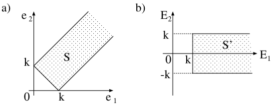
Figure 21: The domains of integration in Eqs. (76) and (79).

Performing the analytic continuation $Q^{R}(\mbox{{\boldmath$k$}},\omega)={\cal Q}(\mbox{{\boldmath$k$}},\nu_{n})|_{i\nu_{n}=\omega+i\eta}$ and using the fact that the domain $S$ is invariant under the exchange of $e_{1}$ and $e_{2}$, we have

$$Q^{R}(\mbox{{\boldmath$k$}},\omega) = \frac{N_{f}(N_{c}-1)}{(2\pi)^{2}k}\int_{S}de_{1}de_{2}$$ (79)

$$\times\left\{[(e_{1}+e_{2})^{2}-k^{2}]\left(\frac{1-2f^{-}(e_{1})}{\omega+2\mu-e_{1}-e_{2}+i\eta}-\frac{1-2f^{+}(e_{1})}{\omega+2\mu+e_{1}+e_{2}+i\eta}\right)\right.$$

$$\left.+2[(e_{1}-e_{2})^{2}-k^{2}]\frac{f^{-}(e_{1})-f^{+}(e_{2})}{\omega+2\mu-e_{1}+e_{2}+i\eta}\right\}$$

$$= \frac{N_{f}(N_{c}-1)}{(2\pi)^{2}k}\int_{S^{\prime}}\frac{dE_{1}dE_{2}}{2}$$

$$\times\left\{(E_{1}^{2}-k^{2})\left(\frac{\tanh\frac{E_{1}+E_{2}-2\mu}{4T}}{\omega+2\mu-E_{1}+i\eta}-\frac{\tanh\frac{E_{1}+E_{2}+2\mu}{4T}}{\omega+2\mu+E_{1}+i\eta}\right)\right.$$

$$\left.+2(E_{2}^{2}-k^{2})\frac{f^{-}(\frac{E_{1}+E_{2}}{2})-f^{+}(\frac{E_{1}-E_{2}}{2})}{\omega+2\mu-E_{2}+i\eta}\right\}.$$

In the second equality, the new variables $E_{1}\equiv e_{1}+e_{2}$ and $E_{2}\equiv e_{1}-e_{2}$ have been introduced for later convenience to obtain the imaginary part of $Q^{R}(\mbox{{\boldmath$k$}},\omega)$.

As explained in the main text(§3), we first calculate the imaginary part ${\cal Q}$ without introducing a cutoff, and then we define the real part using the dispersion relation with a momentum cutoff introduced. From Eq. (79), we have for the imaginary part of $Q^{R}$,

$${\rm Im}Q^{R}(\mbox{{\boldmath$k$}},\omega)$$ (80)

$$= -\pi\frac{N_{f}(N_{c}-1)}{8\pi^{2}k}\int_{k}^{\infty}dE_{1}\int_{-k}^{k}dE_{2}$$

$$\times\left\{(E_{1}^{2}-k^{2})\left(\tanh\textstyle\frac{E_{1}+E_{2}-2\mu}{4T}\delta(\omega+2\mu-E_{1})-\tanh\textstyle\frac{E_{1}+E_{2}+2\mu}{4T}\delta(\omega+2\mu+E_{1})\right)\right.$$

$$\left.+2(E_{2}^{2}-k^{2})\{f(\textstyle\frac{E_{1}+E_{2}}{2}-\mu)-f(\textstyle\frac{E_{1}-E_{2}}{2}+\mu)\}\delta(\omega+2\mu-E_{2})\right\}$$

$$= -\frac{N_{f}(N_{c}-1)}{8\pi k}\left\{\theta(|\omega+2\mu|-k)\int_{-k}^{k}dE_{2}\left[(\omega+2\mu)^{2}-k^{2}\right]\tanh\textstyle\frac{\omega+E_{2}}{4T}\right.$$

$$\left.+2\theta(-|\omega+2\mu|+k)\int_{k}^{\infty}dE_{1}\left[(\omega+2\mu)^{2}-k^{2}\right]\{f(\textstyle\frac{E_{1}+\omega}{2})-f(\textstyle\frac{E_{1}-\omega}{2})\}\right\}$$

$$= -\frac{N_{f}(N_{c}-1)T}{2\pi k}\left[(\omega+2\mu)^{2}-k^{2}\right]\left\{\theta(|\omega+2\mu|-k)\log\frac{\cosh(\omega+k)/4T}{\cosh(\omega-k)/4T}\right.$$

$$\qquad\qquad\qquad\qquad\qquad\qquad\left.+\theta(-|\omega+2\mu|+k)\log\frac{1+{\rm e}^{-(\omega+k)/2T}}{1+{\rm e}^{-(-\omega+k)/2T}}\right\}$$

$$= -\frac{N_{f}(N_{c}-1)T}{2\pi k}\left[(\omega+2\mu)^{2}-k^{2}\right]$$

$$\times\left\{\log\frac{\cosh(\omega+k)/4T}{\cosh(\omega-k)/4T}-\frac{\omega}{2T}\theta(-|\omega+2\mu|+k)\right\}.$$

As stated above, we next define the real part of $Q^{R}$ through the dispersion relation with Eq. (80) for the imaginary part:

$${\rm Re}Q^{R}(\mbox{{\boldmath$k$}},\omega)=-\frac{1}{\pi}{\rm P}\int d\omega^{\prime}\frac{{\rm Im}Q(\mbox{{\boldmath$k$}},\omega)}{\omega-\omega^{\prime}}.$$ (81)

We introduce a cutoff so that the integration of Eq. (81) becomes consistent with the Thouless criterion Eq. (LABEL:eqn:Thouless). With vanishing momentum, Eq. (80) becomes

$${\rm Im}Q^{R}(\mbox{{\boldmath$k$}}\to{\bf 0},\omega)=-\frac{N_{f}(N_{c}-1)}{4\pi}(\omega+2\mu)^{2}\tanh\frac{\omega}{4T}+O(k^{2}).$$ (82)

Substituting this equation into Eq. (81), we have

$${\rm Re}Q^{R}({\bf 0},0)=\frac{N_{f}(N_{c}-1)}{4\pi^{2}}{\rm P}\int d\omega\frac{(\omega+2\mu)^{2}\tanh\frac{\omega}{4T}}{\omega}.$$ (83)

In comparison with Eq. (9), we find that the cutoff should be introduced as in Eq. (32).

Appendix B Analytic Properties of $Q(\mbox{{\boldmath$k$}},\omega)$

In order to find the pole of the response function $D^{R}(\mbox{{\boldmath$k$}},\omega)$, we have to derive the analytic form of $Q^{R}(\mbox{{\boldmath$k$}},\omega)$ in the lower-half complex energy plane, as given in Eq. (35).

We here restate the definitions of $Q(\mbox{{\boldmath$k$}},z)$, $Q^{R}(\mbox{{\boldmath$k$}},z)$ and $Q^{A}(\mbox{{\boldmath$k$}},z)$ in the complex-energy plane $\mathbb{C}$

$$Q(\mbox{{\boldmath$k$}},z)\equiv{\cal Q}(\mbox{{\boldmath$k$}},\nu_{n})|_{i\nu_{n}\to z},$$ (84)

$$Q^{R}(\mbox{{\boldmath$k$}},z)\equiv Q^{R}(\mbox{{\boldmath$k$}},\omega)|_{\omega\to z},$$ (85)

$$Q^{A}(\mbox{{\boldmath$k$}},z)\equiv Q^{A}(\mbox{{\boldmath$k$}},\omega)|_{\omega\to z}.$$ (86)

Because $Q(\mbox{{\boldmath$k$}},z)$ has a cut along the real axis, $Q^{R}(\mbox{{\boldmath$k$}},z)$ ($Q^{A}(\mbox{{\boldmath$k$}},z)$) coincides with $Q(\mbox{{\boldmath$k$}},z)$ only in the upper (lower) half plane $\mathbb{C}^{+}$ ($\mathbb{C}^{-}$):

$$Q(k,z)=Q^{R}(k,z)\qquad\mbox{for}\quad z\in\mathbb{C}^{+},$$

$$Q(k,z)=Q^{A}(k,z)\qquad\mbox{for}\quad z\in\mathbb{C}^{-}.$$ (87)

In this appendix, we wish to find the analytic form of $Q^{R}(\mbox{{\boldmath$k$}},z)$ in $\mathbb{C}^{-}$. To accomplish this, we first evaluate $Q^{R}(\mbox{{\boldmath$k$}},z)$ just below the real axis, at $z=\omega-i\eta$, and then determine $Q^{R}(\mbox{{\boldmath$k$}},z)$ in $\mathbb{C}^{-}$ by analytic continuation. Here, we note that the discontinuity of $Q(\mbox{{\boldmath$k$}},z)$ at the cut along the real axis is characterized by the discontinuity of the imaginary part, that is,

$$\mbox{Re}Q^{R}(k,\omega+i\eta) = \mbox{Re}Q(k,\omega+i\eta)=\mbox{Re}Q(k,\omega-i\eta)=\mbox{Re}Q^{A}(k,\omega-i\eta),$$ (88)

$$\mbox{Im}Q^{R}(k,\omega+i\eta) = \mbox{Im}Q(k,\omega+i\eta)=-\mbox{Im}Q(k,\omega-i\eta)=-\mbox{Im}Q^{A}(k,\omega-i\eta)$$ (89)

$$\equiv I(k,\omega),$$

with $\omega$ being a real variable. We find from Eq. (31) that cuts of $I(\mbox{{\boldmath$k$}},z)\equiv I(\mbox{{\boldmath$k$}},\omega)|_{\omega\to z}$ exist at $\mbox{Im}z=2(2n+1)\pi T$. Hence, this function is analytic in $\mathbb{C}_{I}\equiv\{z\in\mathbb{C}|-2i\pi T<\mbox{Im}z<2i\pi T\}$. Using Eqs.(88) and (89), we find

$$Q^{R}(k,\omega)-iI(k,\omega) = Q^{R}(k,\omega+i\eta)-i{\rm Im}Q^{R}(k,\omega+i\eta)$$ (90)

$$= {\rm Re}Q^{R}(k,\omega+i\eta)={\rm Re}Q^{A}(k,\omega-i\eta)$$

$$= Q^{A}(k,\omega-i\eta)-i{\rm Im}Q^{A}(k,\omega-i\eta),$$

$$= Q(k,\omega-i\eta)+iI(k,\omega),$$

which leads to

$$Q^{R}(k,\omega-i\eta) = Q^{R}(k,\omega+i\eta)$$ (91)

$$= Q(k,\omega-i\eta)+2iI(k,\omega).$$

In the first equality here, we have used the fact that $Q^{R}(\mbox{{\boldmath$k$}},z)$ is a continuous function on the real axis, and Eq. (90) is applied to derive the second equality. Equation (91) implies that we can express $Q^{R}(\mbox{{\boldmath$k$}},z)$ just below the real axis in terms of the functions $Q(\mbox{{\boldmath$k$}},z)$ and $I(\mbox{{\boldmath$k$}},z)$, whose analytic forms in $\mbox{Im}z<0$ are already known. Because both $Q(\mbox{{\boldmath$k$}},z)$ and $I(\mbox{{\boldmath$k$}},z)$ are analytic functions in $\mathbb{C}^{-}\cap\mathbb{C}_{I}$, the analytic form of $Q^{R}$ in this domain can be obtained straightforwardly from the uniqueness theorem of the analytic continuation as

$$Q^{R}(k,z)=Q(k,z)+2iI(k,z),\qquad{\rm for}\quad z\in\mathbb{C}^{-}\cap\mathbb{C}_{I}.$$ (92)

Although Eq. (92) is valid only for ${\rm Im}z>-2\pi T$, this region is sufficient to find the pole.

For vanishing momentum, analytic continuation into the lower half plane is understood as changing the contour of the momentum integration as shown in Fig. 22. In this case, the term originating from the pole integration is added in the lower half plane[8], and we obtain

$$Q^{R}({\bf 0},z\in\mathbb{C}^{-}) = \frac{2N_{f}(N_{c}-1)}{\pi^{2}}\big{[}{\rm P}\int_{-\Lambda}^{\Lambda}k^{2}dk\frac{\tanh\frac{|{\bf k}|-\mu}{2T}}{z-2(|\mbox{{\boldmath$k$}}|-\mu)}$$ (93)

$$-\frac{1}{2}2\pi i(\mu+\frac{z}{2})^{2}\tanh\frac{z}{4T}\big{]}.$$

Equation (93) coincides, of course, with the $k\to 0$ limit of Eq. (92).

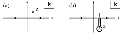
Figure 22: The analytic continuation of $Q^{R}(\mbox{{\boldmath$k$}},\omega)$ for a vanishing momentum.

Appendix C Calculation of $\Sigma$

To carry out the summation of the Matsubara frequency $\omega^{\prime}_{m}$ in Eq. (52), it is sufficient to consider the case $\omega_{n}>0$. Because both $\Xi(\mbox{{\boldmath$k$}},z)$ and $G_{0}(\mbox{{\boldmath$k$}},z)$ have a cut along the real axis, the integrand of Eq. (52) has two cuts along the horizontal lines $\mbox{Im}z=0$ and $\mbox{Im}z=-i\omega_{n}$ in the complex energy plane as shown in Fig. 23. Therefore, we must to separate the Matsubara frequency into four parts to carry out the Matsubara sum in Eq. (52):

$$\tilde{\Sigma}(\mbox{{\boldmath$p$}},\omega_{n}) = 8T\sum_{m}\int\frac{d^{3}\mbox{{\boldmath$q$}}}{(2\pi)^{3}}\tilde{\Xi}(\mbox{{\boldmath$p$}}+\mbox{{\boldmath$q$}},\omega_{n}+\omega_{m}){\cal G}_{0}(\mbox{{\boldmath$q$}},\omega_{m})$$ (94)

$$= 4\int_{C_{1}}\frac{dq^{0}}{2\pi i}\tanh\frac{q^{0}}{2T}\int\frac{d^{3}\mbox{{\boldmath$q$}}}{(2\pi)^{3}}\Xi^{R}(\mbox{{\boldmath$p$}}+\mbox{{\boldmath$q$}},i\omega_{n}+q^{0})G_{0}^{R}(\mbox{{\boldmath$q$}},q^{0})$$

$$+ 4\int_{C_{2}}\frac{dq^{0}}{2\pi i}\tanh\frac{q^{0}}{2T}\int\frac{d^{3}\mbox{{\boldmath$q$}}}{(2\pi)^{3}}\Xi^{R}(\mbox{{\boldmath$p$}}+\mbox{{\boldmath$q$}},i\omega_{n}+q^{0})G_{0}^{A}(\mbox{{\boldmath$q$}},q^{0})$$

$$+ 4\int_{C_{3}}\frac{dq^{0}}{2\pi i}\tanh\frac{q^{0}}{2T}\int\frac{d^{3}\mbox{{\boldmath$q$}}}{(2\pi)^{3}}\Xi(\mbox{{\boldmath$p$}}+\mbox{{\boldmath$q$}},i\omega_{n}+q^{0})G_{0}^{A}(\mbox{{\boldmath$q$}},q^{0})$$

$$+ 4\int_{C_{4}}\frac{dq^{0}}{2\pi i}\tanh\frac{q^{0}}{2T}\int\frac{d^{3}\mbox{{\boldmath$q$}}}{(2\pi)^{3}}\Xi^{A}(\mbox{{\boldmath$p$}}+\mbox{{\boldmath$q$}},i\omega_{n}+q^{0})G_{0}^{A}(\mbox{{\boldmath$q$}},q^{0}),$$

where the contours $C_{1}$ - $C_{4}$ are shown in the left panel of Fig. 23. The definitions of the retarded and advanced T-matrices $\Xi^{R}$ and $\Xi^{A}$ are

$$\Xi(\mbox{{\boldmath$p$}},z) = \Xi^{R}(\mbox{{\boldmath$p$}},z)\quad\mbox{for }z\in\mathbb{C}^{+},$$

$$\Xi(\mbox{{\boldmath$p$}},z) = \Xi^{A}(\mbox{{\boldmath$p$}},z)\quad\mbox{for }z\in\mathbb{C}^{-},$$ (95)

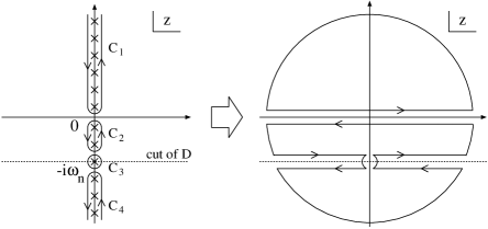
Figure 23: The contours of the $q_{0}$ integrals in Eqs. (94) and (96).

Next, we change the contours $C_{1}$ - $C_{4}$, as shown in Fig. 23. Then the contribution from the integral along the large circle vanishes, and only the integrals along the horizontal lines $\mbox{Im}\omega=0$ and $\mbox{Im}\omega=-i\omega_{n}$ remain. Thus, we have

$$\tilde{\Sigma}(\mbox{{\boldmath$p$}},\omega_{n}) = 4\int\frac{d^{3}\mbox{{\boldmath$q$}}}{(2\pi)^{3}}\int^{\infty}_{-\infty}\frac{dq^{0}}{2\pi i}\tanh\frac{q^{0}}{2T}$$ (96)

$$\times\Xi^{R}(\mbox{{\boldmath$p$}}+\mbox{{\boldmath$q$}},i\omega_{n}+q^{0})\left\{G_{0}^{R}(\mbox{{\boldmath$q$}},q^{0})-G_{0}^{A}(\mbox{{\boldmath$q$}},q^{0})\right\}$$

$$+ 4\int\frac{d^{3}\mbox{{\boldmath$q$}}}{(2\pi)^{3}}\int^{\infty-i\omega_{n}}_{-\infty-i\omega_{n}}\frac{dq^{0}}{2\pi i}\tanh\frac{q^{0}}{2T}$$

$$\times\left\{\Xi^{R}(\mbox{{\boldmath$p$}}+\mbox{{\boldmath$q$}},i\omega_{m}+q^{0})-\Xi^{A}(\mbox{{\boldmath$p$}}+\mbox{{\boldmath$q$}},i\omega_{m}+q^{0})\right\}G_{0}^{A}(\mbox{{\boldmath$q$}},q^{0})$$

$$= 2\int\frac{d^{4}q}{(2\pi)^{4}}\left\{\tanh\frac{q_{0}}{2T}\Xi^{R}(\mbox{{\boldmath$p$}}+\mbox{{\boldmath$q$}},i\omega_{n}+q^{0}){\rm Im}G_{0}^{R}(\mbox{{\boldmath$q$}},q^{0})\right.$$

$$\left.\qquad\qquad+\tanh\frac{q^{0}-i\omega_{n}}{2T}{\rm Im}\Xi^{R}(\mbox{{\boldmath$p$}}+\mbox{{\boldmath$q$}},q^{0})G_{0}^{A}(\mbox{{\boldmath$q$}},q^{0}-i\omega_{n})\right\},\qquad$$

where $\int d^{4}q/(2\pi)^{4}\equiv\int dq^{0}/(2\pi)\int d^{3}\mbox{{\boldmath$q$}}/(2\pi)^{3}$, and the relations

$$\mbox{Im}\Xi^{R}=(\Xi^{R}-\Xi^{A})/2i,\qquad\mbox{Im}G_{0}^{R}=(G_{0}^{R}-G_{0}^{A})/2i$$ (97)

have been used in Eq. (96). It is known that the singularity corresponding to the integral along $C_{3}$ does not give rise to any problem[55]. Then, bearing in mind that $\tanh\frac{\omega-i\omega_{n}}{2T}=\coth\frac{\omega}{2T}$, and employing the analytic continuation $\Sigma^{R}({\mbox{{\boldmath$k$}}},\omega)=\tilde{\Sigma}(\mbox{{\boldmath$k$}},\omega_{n})|_{i\omega_{n}=\omega+i\eta}$, we obtain the self-energy in real time,

$$\Sigma^{R}(\mbox{{\boldmath$k$}},\omega) = 2\int\frac{d^{4}q}{(2\pi)^{4}}\left\{\tanh\frac{q^{0}}{2T}\Xi^{R}(\mbox{{\boldmath$p$}}+\mbox{{\boldmath$q$}},\omega+q^{0}){\rm Im}G_{0}^{R}(\mbox{{\boldmath$q$}},q^{0})\right.$$ (98)

$$\left.\qquad\qquad\qquad+\coth\frac{q^{0}}{2T}{\rm Im}\Xi^{R}(\mbox{{\boldmath$p$}}+\mbox{{\boldmath$q$}},q^{0})G_{0}^{A}(\mbox{{\boldmath$q$}},q^{0}-\omega)\right\}.$$

To simplify Eq. (98) further, we substitute the explicit form of the free Green function,

$$G_{0}^{\{R,A\}}(q)=\frac{\Lambda_{-}(\mbox{{\boldmath$q$}})}{q^{0}+\mu\pm i\eta-|\mbox{{\boldmath$q$}}|}+\frac{\Lambda_{+}(\mbox{{\boldmath$q$}})}{q^{0}+\mu\pm i\eta+|\mbox{{\boldmath$q$}}|},$$ (99)

and its imaginary part,

$$\mbox{Im}G_{0}^{\{R,A\}}(q)=\mp\pi\left(\Lambda_{-}(\mbox{{\boldmath$q$}})\delta(q^{0}+\mu-|\mbox{{\boldmath$q$}}|)+\Lambda_{+}(\mbox{{\boldmath$q$}})\delta(q^{0}+\mu+|\mbox{{\boldmath$q$}}|)\right),$$ (100)

into Eq. (98). Then, Eq. (98) becomes

$$\Sigma_{0}(\mbox{{\boldmath$p$}},\omega) = \frac{1}{4}{\rm Tr}\{\gamma^{0}\Sigma(\mbox{{\boldmath$p$}},\omega)\}$$

$$= -\frac{1}{2}\int\frac{d^{3}\mbox{{\boldmath$q$}}}{(2\pi)^{3}}\int\frac{d\omega}{2\pi}\frac{{\rm Im}~{}\Xi^{R}(\mbox{{\boldmath$p$}}+\mbox{{\boldmath$q$}},\omega)}{\omega-p^{0}-|\mbox{{\boldmath$q$}}|+\mu-i\eta}[\tanh\frac{|\mbox{{\boldmath$q$}}|-\mu}{2T}-\coth\frac{\omega}{2T}]$$

$$-\frac{1}{2}\int\frac{d^{3}\mbox{{\boldmath$q$}}}{(2\pi)^{3}}\int\frac{d\omega}{2\pi}\frac{{\rm Im}~{}\Xi^{R}(\mbox{{\boldmath$p$}}+\mbox{{\boldmath$q$}},\omega)}{\omega-p^{0}+|\mbox{{\boldmath$q$}}|+\mu-i\eta}[\tanh\frac{-|\mbox{{\boldmath$q$}}|-\mu}{2T}-\coth\frac{\omega}{2T}],$$

$$\Sigma_{\rm v}(\mbox{{\boldmath$p$}},\omega) = -\frac{1}{4}{\rm Tr}\{(\hat{\mbox{{\boldmath$p$}}}\cdot\mbox{{\boldmath$\gamma$}})\Sigma(\mbox{{\boldmath$p$}},\omega)\}$$

$$= -\int\frac{d^{3}\mbox{{\boldmath$q$}}}{(2\pi)^{3}}\int\frac{d\omega}{2\pi}\frac{{\rm Im}~{}\Xi^{R}(\mbox{{\boldmath$p$}}+\mbox{{\boldmath$q$}},\omega)}{\omega-p^{0}-|\mbox{{\boldmath$q$}}|+\mu-i\eta}(\hat{\mbox{{\boldmath$q$}}}\cdot\hat{\mbox{{\boldmath$p$}}})[\tanh\frac{|\mbox{{\boldmath$q$}}|-\mu}{2T}-\coth\frac{\omega}{2T}]$$

$$+\int\frac{d^{3}\mbox{{\boldmath$q$}}}{(2\pi)^{3}}\int\frac{d\omega}{2\pi}\frac{{\rm Im}~{}\Xi^{R}(\mbox{{\boldmath$p$}}+\mbox{{\boldmath$q$}},\omega)}{\omega-p^{0}+|\mbox{{\boldmath$q$}}|+\mu-i\eta}(\hat{\mbox{{\boldmath$q$}}}\cdot\hat{\mbox{{\boldmath$p$}}})[\tanh\frac{-|\mbox{{\boldmath$q$}}|-\mu}{2T}-\coth\frac{\omega}{2T}].$$

The imaginary parts of these quantities are found to be

$${\rm Im}~{}\Sigma_{0}(\mbox{{\boldmath$p$}},p^{0})$$ (103)

$$= -\frac{1}{4}\int\frac{d^{3}\mbox{{\boldmath$q$}}}{(2\pi)^{3}}{\rm Im}~{}\Xi^{R}(\mbox{{\boldmath$p$}}+\mbox{{\boldmath$q$}},p^{0}+|\mbox{{\boldmath$q$}}|-\mu)[\tanh\textstyle\frac{|{\mbox{{\boldmath$q$}}}|-\mu}{2T}-\coth\frac{p^{0}+|{\mbox{{\boldmath$q$}}}|-\mu}{2T}]$$

$$-\frac{1}{4}\int\frac{d^{3}\mbox{{\boldmath$q$}}}{(2\pi)^{3}}{\rm Im}~{}\Xi^{R}(\mbox{{\boldmath$p$}}+\mbox{{\boldmath$q$}},p^{0}-|\mbox{{\boldmath$q$}}|-\mu)[\tanh\textstyle\frac{-|{\mbox{{\boldmath$q$}}}|-\mu}{2T}-\coth\frac{p^{0}-|{\mbox{{\boldmath$q$}}}|-\mu}{2T}],$$

$${\rm Im}~{}\Sigma_{\rm v}(\mbox{{\boldmath$p$}},p^{0})$$

$$= -\frac{1}{4}\int\frac{d^{3}\mbox{{\boldmath$q$}}}{(2\pi)^{3}}{\rm Im}~{}\Xi^{R}(\mbox{{\boldmath$p$}}+\mbox{{\boldmath$q$}},p^{0}+|\mbox{{\boldmath$q$}}|-\mu)(\hat{\mbox{{\boldmath$q$}}}\cdot\hat{\mbox{{\boldmath$p$}}})[\tanh\textstyle\frac{|{\mbox{{\boldmath$q$}}}|-\mu}{2T}-\coth\textstyle\frac{p^{0}+|{\bf q}|-\mu}{2T}]$$

$$+\frac{1}{4}\int\frac{d^{3}\mbox{{\boldmath$q$}}}{(2\pi)^{3}}{\rm Im}~{}\Xi^{R}(\mbox{{\boldmath$p$}}+\mbox{{\boldmath$q$}},p^{0}-|\mbox{{\boldmath$p$}}|-\mu)(\hat{\mbox{{\boldmath$q$}}}\cdot\hat{\mbox{{\boldmath$p$}}})[\tanh\textstyle\frac{-|{\mbox{{\boldmath$q$}}}|-\mu}{2T}-\coth\textstyle\frac{p^{0}-|{\mbox{{\boldmath$p$}}}|-\mu}{2T}].$$

References

- [1] K. Rajagopal and F. Wilczek, Chapter 35 in the Festschrift in honor of B. L. Ioffe, ”At the Frontier of Particle Physics / Handbook of QCD”, M. Shifman, ed., (World Scientific); M. Alford, Ann. Rev. Nucl. Part. Sci. 51,131 (2001); T. Schafer, hep-ph/0304281; D. H. Rischke, Prog. Part. Nucl. Phys. 52, 197 (2004).
- [2] J. C. Collins and M. J. Perry, Phys. Rev. Lett. 34, 1353 (1975).
- [3] B. C. Barrois, Nucl. Phys. B129, 390 (1977).
- [4] D. Bailin and A. Love, Phys. Rept. 107, 325 (1984).
- [5] K. Rajagopal, E. Shuster, Phys.Rev. D62, 085007 (2000).
- [6] M. G. Alford, K. Rajagopal and F. Wilczek, Nucl. Phys. B537, 443 (1999).
- [7] D. Blaschke, T. Klahn, D.N. Voskresensky, Astrophys. J. 533, 406 (2000); M. Alford and S. Reddy, Phys. Rev. D67,074024 (2003); H. Grigorian, D. Blaschke, D. Voskresensky, Phys. Rev. C71 (2005), 045801.
- [8] M. Kitazawa, T. Koide, T. Kunihiro and Y. Nemoto, Phys. Rev. D65, 091504(R) (2001).
- [9] D. N. Voskresensky, Phys. Rev. C69, 065209 (2004).
- [10] K. Iida and G. Baym, Phys. Rev. D63, 074018 (2001); Erratum-ibid. D66, 059903 (2002).
- [11] M. Alford, J. Berges and K. Rajagopal, Nucl. Phys. B558, 219 (1999).
- [12] A. W. Steiner, S. Reddy and M. Prakash, Phys. Rev. D66, 094007 (2002).
- [13] I. Shovkovy and M. Huang, Phys. Lett. B564, 205 (2003).
- [14] E. Gubankova, W.V. Liu and F. Wilczek, Phys. Rev. Lett. 91, 032001 (2003).
- [15] M. Huang and I. Shovkovy, Nucl. Phys. A729, 835 (2003).
- [16] M. Alford, C. Kouvaris and K. Rajagopal, Phys. Rev. Lett. 92,222001 (2004).
- [17] K. Iida, T. Matsuura, M. Tachibana and T. Hatsuda, Phys. Rev. Lett. 93, 132001 (2004).
- [18] S. B. Ruster, I. A. Shovkovy and D. H. Rischke, Nucl. Phys. A743, 127 (2004).
- [19] K. Fukushima, C. Kouvaris and K. Rajagopal, Phys. Rev. D71 (2005), 034002.
- [20] H. Abuki, M. Kitazawa and T. Kunihiro, Phys. Lett. B615 (2005), 102.
- [21] M. Matsuzaki, Phys. Rev. D62, 017501 (2000).
- [22] H. Abuki, T. Hatsuda and K. Itakura, Phys. Rev. D65, 074014 (2002).
- [23] G.E. Brown, C.-H. Lee, M. Rho and E. Shuryak, Nucl. Phys. A740, 171 (2004); E.V. Shuryak and I. Zahed, Phys. Rev. C70, 021901 (2004); R. Stock, J. Phys. G: Nucl. Part. Phys. 30, S633 (2004), Quark Matter 2004, proceedings of the 17th international conference on ultra-relativistic nucleus-nucleus collisions.
- [24] T. Hatsuda and T. Kunihiro, Phys. Lett. B145, 7 (1984); Phys. Rev. Lett. 55, 158 (1985).
- [25] C. DeTar, Phys. Rev. D32, 276 (1985).
- [26] T. Umeda, K. Nomura and H. Matsufuru, Eur. Phys. J. C39S1 (2005),16; M. Asakawa and T. Hatsuda, Phys. Rev. Lett. 92, 012001 (2004); S. Datta, F. Karsch, P. Petreczky and I. Wetzorke, Phys. Rev. D69, 094507 (2004); see also T. Umeda, R. Katayama, O. Miyamura and H. Matsufuru, Int. J. Mod. Phys. A16, 2215 (2001).
- [27] M. Kitazawa, T. Koide, T. Kunihiro and Y. Nemoto, Phys. Rev. D70, 056003 (2004).
- [28] As a experimental review, T. Timusk and B. Statt, Rep. Progr. Phys. 62, 61 (1999).
- [29] V.M. Loktev, R.M. Quick and S.G. Sharapov, Phys. Rep. 349, 1 (2001), and references therein.
- [30] Y. Yanase, T. Jujo, T. Nomura, H. Ikeda, T. Hotta and K. Yamada, Phys. Rep. 387, 1 (2003).
- [31] T. Matsuura, K. Iida, T. Hatsuda and G. Baym, hep-ph/0312363.
- [32] I. Giannakis, D. f. Hou, H. c. Ren and D. H. Rischke, Phys. Rev. Lett. 93, 232301 (2004).
- [33] See also, R. D. Pisarski, Phys. Rev. C62, 035202 (2000); S. Mo, J. Hove and A. Sudbø, Phys. Rev. B65, 104501 (2002).
- [34] I. Giannakis and H.-c. Ren, Nucl.Phys. B669,462 (2003).
- [35] A. Nakamura, T. Hatsuda, A. Hosaka and T. Kunihiro, Prog. Theor. Phys. Suppl. 153 (2004), prepared for workshop on Finite Density QCD at Nara, Nara, Japan, 10-12 Jul 2003.
- [36] T. Schäfer and E. Shuryak, Rev. Mod. Phys. 70, 323 (1998).
- [37] T. Hatsuda and T. Kunihiro, Phys. Rep. 247, 221 (1994).
- [38] M. Buballa, Phys. Rep. 407 (2005), 205.
- [39] J. Berges and K. Rajagopal, Nucl. Phys. B538, 215 (1999).
- [40] T.M. Schwarz, S.P. Klevansky and G. Papp, Phys. Rev. C60, 055205 (1999).
- [41] M. Kitazawa, T. Koide, T. Kunihiro and Y. Nemoto, Prog. Theor. Phys. 106, 929.
- [42] R. Rapp, T. Schäfer, E. Shuryak and M. Velkovsky, Phys. Rev. Lett. 81, 53 (1998); Ann. Phys. 280, 35 (2000).
- [43] N. Evans, S.D.H. Hsu and M. Schwetz, Nucl. Phys. B551, 275 (1999); T. Schafer and F. Wilczek, Phys. Lett. B450, 325 (1999).
- [44] M. Harada and S. Takagi, Prog. Theor. Phys. 107, 561 (2002); S. Takagi, Prog. Theor. Phys. 109, 233 (2003).
- [45] E. Babaev, Phys. Rev. D62, 074020 (2000); Int. J. Mod. Phys. A16, 1175 (2001); K. Zarembo, JETP Lett. 75, 59 (2002).
- [46] S.P. Klevansky, Rev. Mod. Phys. 64, 649 (1992).
- [47] R. Alkofer and L. von Smekal, Phys. Rep. 353, 281 (2001).
- [48] W. Bentz and A. W. Thomas, Nucl. Phys. A696, 138 (2001).
- [49] H. Mineo, W. Bentz and K. Yazaki, Nucl. Phys. A684, 293 (2001).
- [50] L. van Hove, Phys. Rev. 95, 249 (1954).
- [51] D.J. Thouless, Ann. Phys. 10, 553 (1960).
- [52] Y. Nambu and G. Jona-Lasinio, Phys. Rev. 122, 345 (1961); 124, 246 (1961).
- [53] S. Klimt, M. Lutz, U. Vogl and W. Weise, Nucl. Phys. A516, 429 (1990).
- [54] M. Cyrot, Rep. Prog. Phys. 36, 103 (1973).
- [55] A.A. Abrikosov, L.P. Gorkov, and I.E.Dzyaloshinski, Methods of Quantum Field Theory in Statistical Physics.
- [56] M. Kitazawa and T. Kunihiro, in preparation.
- [57] A. P. Levanyuk, Sov. Phys. JETP 9, 571 (1959).
- [58] V. L. Ginzburg, Sov. Phys. Solid state 2, 1824 (1960).
- [59] see, for example, L. D. Landau and E. M. Lifshiz, Statistical Physics (Pergamon, New York, 1958).
- [60] L.P. Kadanoff and G. Baym, Quantum statistical mechanics,( W.A. Benjamin, 1962).
- [61] K. Maki, Prog. Theor. Phys. 39, 897 (1968).
- [62] H. Takayama, Prog. Theor. Phys. 43, 1445 (1970);
- [63] E. Abrahams, M. Redi, J. W. F. Woo, Phys. Rev. B 1, 208 (1970).
- [64] B. Jankö, J. Maly and K. Levin, Phys. Rev. B56, R11 407 (1997).
- [65] A. Schnell, G. Röpke and P. Schuck, Phys. Rev. Lett. 83, 1926 (1999).
- [66] L.G. Aslamazov and A.I. Larkin, Sov. Phys. Solid State 10, 875 (1968).
- [67] K. Maki, Prog. Theor. Phys. 40, 193 (1968); R.S. Thompson, Phys. Rev. B1, 327 (1970).
- [68] S. Fujimoto, J. Phys. Soc. Jpn. 71, 1230 (2002).
- [69] M. Kitazawa, T. Kunihiro and Y. Nemoto, hep-ph/0505070.