Kaluza-Klein masses of bulk fields
with general boundary conditions in AdS₅

Abstract

Recently bulk Randall-Sundrum theories with the gauge group $SU(2)_{L}\times SU(2)_{R}\times U(1)_{B-L}$ have drawn a lot of interest as an alternative to electroweak symmetry breaking mechanism. These models are in better agreement with electroweak precision data since custodial isospin symmetry on the IR brane is protected by the extended bulk gauge symmetry. We comprehensively study, in the $S^{1}/\mathbb{Z}_{2}\times\mathbb{Z}_{2}^{\prime}$ orbifold, the bulk gauge and fermion fields with the general boundary conditions as well as the bulk and localized mass terms. Master equations to determine the Kaluza-Klein (KK) mass spectra are derived without any approximation, which is an important basic step for various phenomenologies at high energy colliders. The correspondence between orbifold boundary conditions and localized mass terms is demonstrated not only in the gauge sector but also in the fermion sector. As the localized mass increases, the first KK fermion mass is shown to decrease while the first KK gauge boson mass to increase. The degree of gauge coupling universality violation is computed to be small in most parameter space, and its correlation with the mass difference between the top quark and light quark KK mode is also studied.

I Introduction

The origin of electroweak symmetry breaking (EWSB) has still remained to be explored by experiments. In the standard model (SM), EWSB occurs spontaneously as the Higgs field develops vacuum expectation value (VEV). This Higgs mechanism is, however, regarded unsatisfactory since the Higgs potential is introduced just for the purpose of EWSB itself. Furthermore it is extremely unstable against radiative corrections and thus UV physics, creating the so-called gauge hierarchy problem. Most of models for new physics beyond the SM pursue more natural EWSB mechanism. According to symmetry breaking coupling strength, new models are divided into two classes: One is a weakly coupled theory with a high cut-off scale and the other is a strongly coupled theory dynamical .

Recently it is shown that these two different classes can be related by AdS/CFT duality Maldacena:1997re ; Gubser:1998bc ; Witten:1998qj ; Aharony:1999ti : A four-dimensional (4D) theory with a strongly coupled sector conformal from the Planck scale to the weak scale is dual to a 5D weakly coupled Randall-Sundrum model-1 (RS1) Randall:1999ee ; Randall:1999vf ; Arkani-Hamed:2000ds ; Rattazzi:2000hs ; Perez-Victoria:2001pa . The RS1 model has one extra spatial dimension of a truncated AdS space, the orbifold of $S^{1}/\mathbb{Z}_{2}\times\mathbb{Z}_{2}^{\prime}$ without the assumption of periodic boundary condition. The fixed point under $\mathbb{Z}_{2}$ parity transformation is called the UV brane and that under $\mathbb{Z}_{2}^{\prime}$ parity the IR brane. In the original RS scenario, all the SM fields are confined on the TeV brane Randall:1999ee . Since a localized field in the 5D theory is dual to the TeV-scale composite in the strong sector of the 4D theory, the phenomenological aspects of a localized field depend sensitively on the unknown UV physics. This feature aroused great interest in bulk RS theories Davoudiasl:1999tf ; Chang:1999nh ; Kim:2002kk ; Grossman:1999ra ; Gherghetta:2000qt ; Huber:2000fh ; Huber:2000ie . As weakly coupled effective field theories, their phenomenological implications become more reliable. For example it is feasible to discuss the RG running of gauge couplings and their unification Pomarol:2000hp ; Goldberger:2002hb ; Agashe:2002bx ; Contino:2002kc ; Randall:2001gb ; Randall:2001gc ; Choi:2002ps ; Agashe:2002pr ; Goldberger:2002pc ; KChoi . To solve the gauge hierarchy problem, however, the Higgs field should be localized on the IR-brane.

A naive extension of the RS1 model by releasing the SM gauge and fermion fields in the bulk, however, has troubles with electroweak precision data, particularly with the Peskin-Takeuchi $T$ parameter Csaki:2002gy ; Hewett:2002fe ; Burdman:2002gr . This problem is attributed to the lack of isospin custodial symmetry. Recently a bulk gauge symmetry of $SU(2)_{R}$ has been added, which is used to restore a gauge version of custodial symmetry in the bulk Agashe:2003zs ; Burdman:2004rz . Another rather radical solution to EWSB in this framework is the Higgsless theory: The gauge symmetry breaking is due to non-trivial orbifold boundary conditions. Non-zero SM gauge boson masses are nothing but the first Kaluza-Klein (KK) mode mass Csaki:2003dt ; Csaki:2003sh ; Csaki:2003zu . From the AdS/CFT correspondence, we can interpret this model as a dual of a technicolor model.

Both models with Agashe:2003zs and without Csaki:2003dt a Higgs boson incorporate two kinds of new ingredients in the phenomenological view point. First, we have new gauge fields $\overrightarrow{W}^{\mu}_{R}$ of $SU(2)_{R}$, introduced for the custodial isospin symmetry. At high energy colliders, they appear as KK excitations with TeV scale masses since the $\mathbb{Z}_{2}\times\mathbb{Z}_{2}^{\prime}$ parity of $\overrightarrow{W}^{\mu}_{R}$ is not $(++)$. Secondly, new bulk fermions are also required. The $SU(2)_{R}$ symmetry, which promotes the SM right-handed fermions to the doublets, is broken by the UV orbifold boundary conditions: in the Agashe-Delgado-May-Sundrum (ADMS) model Agashe:2003zs , for example, ${W}^{\pm}_{R}$ fields have definite $(-+)$ parity; the SM right-handed up quark with $(++)$ parity should couple with a new right-handed down-type quark with $(-+)$ parity for $\mathbb{Z}_{2}\times\mathbb{Z}_{2}^{\prime}$ invariant action.

Since the bulk RS models with custodial isospin symmetry are compatible with electroweak precision data, its phenomenological probe should await experiments at future colliders Barbieri:2004qk ; Barbieri:2003pr ; Nomura:2003du ; Foadi:2003xa ; Davoudiasl:2003me ; Davoudiasl:2004pw ; Burdman:2003ya ; Cacciapaglia:2004jz ; Cacciapaglia:2004rb ; Birkedal:2004au . Exact KK mass spectra of the bulk gauge boson and fermion are of great significance. In the ADMS model where the $\mathbb{Z}_{2}\times\mathbb{Z}_{2}^{\prime}$ parity is conserved at tree level, for example, the decay of new gauge bosons with $(-+)$ parity into the SM particles with $(++)$ parity can be limited and thus long-lived. We will derive, without any approximation, master equations for the KK masses particularly with the general localized mass terms. Special focus is on the KK masses of the top quark, on which the effect of the localized Yukawa coupling is significant. Contrary to the gauge bosons case, the first KK mode mass of top quark decreases with increasing top Yukawa coupling. We will also suggest a phenomenologically dramatic case, called the KK mode degenerate case, where the first and second KK masses of fermions are degenerate without the localized Yukawa coupling. Another interesting feature of this case is that the mass drop of the first KK mode by the localized Yukawa coupling is maximized. It is very feasible, therefore, that the first signal of KK fermion comes from the top quark mode.

It is also worthwhile to distinguish the role of UV-brane localized VEV (parameterized by a dimensionless parameter $a_{{}_{\rm UV}}$) and that of IR-brane localized VEV (parameterized by $a_{{}_{\rm IR}}$) in the generation of the zero-mode mass of a gauge boson with (++) parity. Generically either $a_{{}_{\rm UV}}$ or $a_{{}_{\rm IR}}$ generates TeV scale mass for the zero mode, which would vanish with $a_{{}_{\rm UV}}=a_{{}_{\rm IR}}=0$. We will show that quite different is the way to generate the zero mode mass: $a_{{}_{\rm IR}}$ gradually increases the zero-mode mass, while even small $a_{{}_{\rm UV}}$ (but larger than about $10^{-15}$) lifts up the zero-mode mass to TeV scale at one stroke.

Another interesting issue is the theoretical relation between the Higgsless model and the ADMS model. This correspondence in the gauge sector was pointed out in Ref. Nomura:2003du . Similar correspondence in the bulk fermion sector is deserved to study also. Based on the exact formulae of KK masses, we will show that the bulk fermion field with non-trivial orbifold boundary conditions in the Higgsless theory can be understood through the VEV of a localized scalar field. This will complete the understanding of orbifold boundary conditions.

Inevitable deviation of gauge coupling unification, denoted by $\delta g_{Wtb}$, shall be studied. We will focus on its correlation with the top quark mass spectra. If this correlation is strong enough, it can be a valuable information since the magnitude of $\delta g_{Wtb}$ in most parameter space is too small to be probed at hadron colliders. Restricted to the KK mode degenerate case, we will show a significant correlation between the $\delta g$ and the top quark KK mode mass relative to light quark KK mode mass.

This paper is organized as follows. In Sec. II, we give the general setup for the bulk gauge boson. By solving wave equations with the brane localized mass terms, we derive the master equations for the KK masses. The interpolation between the ADMS model and the Higgsless model are to be understood as a consequence of master equations in a limiting case. Some numerical values of KK states are also presented. Section III deals with the KK masses of a bulk fermion without the brane localized mass term. More delicate case with the brane localized Yukawa coupling is considered in Sec. IV. The possibility of gauge coupling universality violation is also studied in Sec. V, which arises due to the deviation of KK zero mode functions by brane localized masses. In Sec. VI, we present the summary and conclusions.

II Bulk gauge bosons

Figure 1: The $S^{1}/\mathbb{Z}_{2}\times\mathbb{Z}_{2}^{\prime}$ orbifold.

We consider a gauge theory in a five-dimensional warped spacetime with the metric given by

$$ds_{5}^{2}\equiv g_{MN}dx^{M}dx^{N}=e^{-2\sigma(y)}(dt^{2}-d\vec{x}\,^{2})-dy^{2},$$ (1)

where $y$ is the fifth dimension coordinate and $\sigma(y)=k|y|$. The theory is to be compactified on the $S^{1}/\mathbb{Z}_{2}\times\mathbb{Z}_{2}^{\prime}$ orbifold, which is a circle of radius $r_{c}$ with two reflection symmetries under $\mathbb{Z}_{2}:y\to-y$ and $\mathbb{Z}_{2}^{\prime}:y^{\prime}\to-y^{\prime}$ $(y^{\prime}=y-\pi r_{c}/2)$ as depicted in Fig. 1. Often the conformal coordinate of $z\equiv e^{\sigma}/k$ is useful:

$$ds_{5}^{2}=\frac{1}{(kz)^{2}}\left(dt^{2}-d\vec{x}\,^{2}-dz^{2}\right).$$ (2)

Since $y$ is confined in $0\leq y\leq L~{}(L\equiv\pi r_{c}/2)$, $z$ is also bounded in $1/k\leq z\leq 1/T$. Here $T$ is the effective electroweak scale, defined by $T\equiv e^{-kL}k\equiv\epsilon\,k$. With $kL\approx 35$, the warp factor $\epsilon(\equiv e^{-kL})$ reduces $T$ at TeV scale from $k$ at Planck scale: With this scaling the gauge hierarchy problem is answered. The space of $S^{1}/\mathbb{Z}_{2}\times\mathbb{Z}_{2}^{\prime}$ accommodates two fixed points, the $\mathbb{Z}_{2}$ fixed point at $z_{{}_{\rm UV}}=1/k$ (called the UV brane) and the $\mathbb{Z}_{2}^{\prime}$ fixed point at $z_{{}_{\rm IR}}=1/T$ (called the IR brane).

The action for a 5D $U(1)$ gauge field is

$$S_{\mathrm{gauge}}=\int d^{4}xdz\sqrt{G}\left[-\frac{1}{4}g^{MP}g^{NQ}F_{MN}F_{PQ}+\frac{1}{2}M^{2}g^{MN}A_{M}A_{N}\right],$$ (3)

where $G$ is the determinant of the AdS metric, $F_{MN}=\partial_{M}A_{N}-\partial_{N}A_{M}$. The general mass term $M^{2}(z)$, including the case where the gauge symmetry is broken in the bulk, is

$$M^{2}(z)=a_{{}_{\rm UV}}^{2}k\,\delta(z-z_{{}_{\rm UV}})+a_{{}_{\rm IR}}^{2}k\,\delta(z-z_{{}_{\rm IR}})+b^{2}k^{2},$$ (4)

where the dimensionless $b$ and $a_{{}_{\rm UV}}(a_{{}_{\rm IR}})$ parameterize the bulk mass and the localized mass on the UV (IR) brane, respectively. Note that $b$ breaks the gauge symmetry.

The KK expansion of the dimension 3/2 field $A^{M}(x,z)$ is

$$A_{\nu}(x,z)=\sqrt{k}\sum_{n}A_{\nu}^{(n)}(x){f_{A}^{(n)}}(z),$$ (5)

where the mode function ${f_{A}^{(n)}}(z)$ is dimensionless. With the following equation of motion for ${f_{A}^{(n)}}(z)$

$$-z\partial_{z}\left(\frac{1}{z}\partial_{z}{f_{A}^{(n)}}(z)\right)+\frac{M^{2}(z)}{k^{2}z^{2}}{f_{A}^{(n)}}(z)={m_{A}^{(n)}}^{2}{f_{A}^{(n)}}(z),$$ (6)

and the normalization of

$$\int\frac{dz}{z}f_{A}^{(n)}f_{A}^{(m)}=\delta_{nm}\,,$$ (7)

the action in Eq. (3) describes a tower of massive KK gauge bosons:

$$S_{\mathrm{gauge}}=\sum_{n}\int d^{4}x\left[-\frac{1}{4}\eta^{\mu\rho}\eta^{\nu\kappa}F^{(n)}_{\mu\nu}F^{(n)}_{\rho\kappa}-m_{A}^{(n)}\eta^{\mu\nu}A^{{(n)}}_{\mu}A^{(n)}_{\nu}\right]\,,$$ (8)

where $F^{(n)}_{\mu\nu}=\partial_{\mu}A^{(n)}_{\nu}-\partial_{\nu}A^{(n)}_{\mu}$. The general solution of Eq. (6) in the bulk ($z_{{}_{\rm UV}}<z<z_{{}_{\rm IR}}$) is

$${f_{A}^{(n)}}(z)=\frac{z}{N_{A}^{(n)}}\left[J_{\nu}({m_{A}^{(n)}}z)+\beta_{A}^{(n)}Y_{\nu}({m_{A}^{(n)}}z)\right],$$ (9)

where $\nu=\sqrt{1+b^{2}}$ and $N_{A}^{(n)}$ is determined by the normalization condition in Eq. (7).

Boundary conditions on the two branes specify the constant $\beta_{A}^{(n)}$. If the mode function $f_{A}^{(n)}(z)$ has $\mathbb{Z}_{2}$- or $\mathbb{Z}_{2}^{\prime}$-even parity, Neumann boundary condition applies as

$$\left.\frac{d{f_{A}^{(n)}}}{dz}\right|_{z=z_{i}}=(-1)^{P_{i}}\frac{a_{i}^{2}}{2}f^{(n)}|_{z=z_{i}},\quad i={\mathrm{UV},~{}\mathrm{IR}}$$ (10)

where $P_{\rm UV}=2$, and $P_{\rm IR}=1$. The sign difference between the UV and IR brane is due to the directionality of the derivative at the boundary points. Here physics is essentially similar to the case where the electric field near the conducting boundary is determined by the charge localized on the conducting plane. For $\mathbb{Z}_{2}$- or $\mathbb{Z}_{2}^{\prime}$-even function, the $\beta_{A}^{(n)}$ coefficient is

$$-\beta_{A}^{(n)}\mid_{\rm even} = \frac{\left(-(-1)^{P_{i}}\frac{a_{i}^{2}}{2}+1-\nu\right)J_{\nu}({m_{A}^{(n)}}z_{i})+{m_{A}^{(n)}}z_{i}J_{\nu-1}({m_{A}^{(n)}}z_{i})}{\left(-(-1)^{P_{i}}\frac{a_{i}^{2}}{2}+1-\nu\right)Y_{\nu}({m_{A}^{(n)}}z_{i})+{m_{A}^{(n)}}z_{i}Y_{\nu-1}({m_{A}^{(n)}}z_{i})}$$

$$\equiv R_{N}(a_{i},\nu,{m_{A}^{(n)}}z_{i}).$$

If the function ${f_{A}^{(n)}}$ has $\mathbb{Z}_{2}$- or $\mathbb{Z}_{2}^{\prime}$-odd parity at the corresponding boundary, the Dirichlet boundary condition applies as

$$\left.{f_{A}^{(n)}}\right|_{z=z_{i}}=0\,.$$ (12)

Their $\beta_{A}^{(n)}$’s are

$$-\left.\beta_{A}^{(n)}\right|_{\rm odd}=\frac{J_{\nu}({m_{A}^{(n)}}z_{i})}{Y_{\nu}({m_{A}^{(n)}}z_{i})}\equiv R_{D}(\nu,{m_{A}^{(n)}}z_{i}).$$ (13)

Note that the Dirichlet boundary condition is independent of the localized mass term $a_{{}_{\rm UV,IR}}$.

In the $S^{1}/\mathbb{Z}_{2}\times\mathbb{Z}_{2}^{\prime}$ orbifold, four different $\mathbb{Z}_{2}\times\mathbb{Z}_{2}^{\prime}$ parities are possible as $(++),(+-),(-+)$ and $(--)$. Since two boundary conditions doubly constrain a single constant $\beta_{A}^{(n)}$ coefficient, the KK mass ${m_{A}^{(n)}}$ is determined by the following master equations:

$$\bullet~{}~{}(++):\quad R_{N}(a_{{}_{\rm UV}},\nu,{m_{A}^{(n)}}z_{{}_{\rm UV}}) = R_{N}(a_{{}_{\rm IR}},\nu,{m_{A}^{(n)}}z_{{}_{\rm IR}}),$$ (14)

$$\bullet~{}~{}(+-):\quad R_{N}(a_{{}_{\rm UV}},\nu,{m_{A}^{(n)}}z_{{}_{\rm UV}}) = R_{D}(\nu,{m_{A}^{(n)}}z_{{}_{\rm IR}}),$$ (15)

$$\bullet~{}~{}(-+):\quad\hskip 24.0ptR_{D}(\nu,{m_{A}^{(n)}}z_{{}_{\rm UV}}) = R_{N}(a_{{}_{\rm IR}},\nu,{m_{A}^{(n)}}z_{{}_{\rm IR}}),$$ (16)

$$\bullet~{}~{}(--):\quad\hskip 24.0ptR_{D}(\nu,{m_{A}^{(n)}}z_{{}_{\rm UV}}) = R_{D}(\nu,{m_{A}^{(n)}}z_{{}_{\rm IR}})\,.$$ (17)

From the functional forms of $R_{N}$ and $R_{D}$, the $\mathbb{Z}_{2}\times\mathbb{Z}_{2}^{\prime}$ parity can be understood through the effect of large localized Higgs VEV. In the large $a_{i}$ limit, $R_{N}$ approaches $R_{D}$:

$$\lim_{a_{i}\rightarrow\infty}R_{N}(a_{i},\nu,{m_{A}^{(n)}}z_{i})=\lim_{a_{i}\rightarrow\infty}\frac{-(-1)^{P}\frac{a_{i}^{2}/}{2}J_{\nu}({m_{A}^{(n)}}z_{i})}{-(-1)^{P}\frac{a_{i}^{2}/}{2}Y_{\nu}({m_{A}^{(n)}}z_{i})}=R_{D}(\nu,{m_{A}^{(n)}}z_{i}).$$ (18)

This happens because the 5D wave function is expelled by large VEV of the localized Higgs field. In the large $a_{i}$ limit, therefore, the KK masses of the $\mathbb{Z}_{2}$- or $\mathbb{Z}_{2}^{\prime}$-even gauge field become identical with those of $\mathbb{Z}_{2}$- or $\mathbb{Z}_{2}^{\prime}$-odd field. For example, the KK masses of a $(++)$ gauge field with large $a_{{}_{\rm UV}}$ are the same as that of a $(-+)$ field without localized mass. Usually this behavior is expressed that the $(++)$ gauge field mimics $(-+)$ field. Similarly, the $(++)$ gauge field with large $a_{{}_{\rm IR}}$ mimics the $(+-)$ field; the $(++)$ field with both large $a_{{}_{\rm UV}}$ and $a_{{}_{\rm IR}}$ mimics the $(--)$ field. Figure 2 summarizes all the correspondences. These relations could be interpreted as the origin of the interpolation between the ADMS model and the Higgsless model in the AdS dual picture.

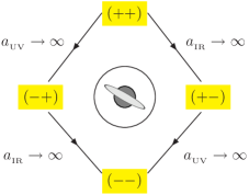
Figure 2: Diagram shows relationship between different boundary conditions by dialing vacuum expectation value of localized Higgs fields. This is the underlying physics in the interpolation between the theories of gauge symmetry breaking by a localized Higgs field and by a technicolor-like strong dynamics in the AdS dual picture.

For the numerical calculation, we assume the bulk mass parameter $b$ to be zero. In Fig. 3, we present the KK masses of a bulk gauge boson in unite of $T$ without any localized masses, i.e., $a_{{}_{\rm UV}}=a_{{}_{\rm IR}}=0$. The RS metric alone determines the KK mass spectra. It is clear that only the bulk gauge boson with $(++)$ parity allows zero mode. A remarkable feature is the substantially light mass of the first KK mode with $(+-)$ parity. With $T\sim$TeV, $m_{A(+-)}^{(1)}$ can be of order 100 GeV. Since the $(+-)$ parity mode is equivalent to the $(++)$ parity mode in the limit of large $a_{{}_{\rm IR}}$, this feature suggests the possibility of the gauge symmetry breaking by orbifold boundary conditions without the Higgs mechanism. Numerically we have

$${m_{A(++)}^{(1)}} \approx 2.45\,{T},\quad{m_{A(++)}^{(2)}}\approx 5.57\,{T},\quad{m_{A(++)}^{(3)}}\approx 8.70\,{T},$$ (19)

$${m_{A(+-)}^{(1)}} \approx 0.24\,{T},\quad{m_{A(+-)}^{(2)}}\approx 3.88\,{T},\quad{m_{A(+-)}^{(3)}}\approx 7.06\,{T},$$

$${m_{A(-+)}^{(1)}} \approx 2.40\,{T},\quad{m_{A(-+)}^{(2)}}\approx 5.52\,{T},\quad{m_{A(-+)}^{(3)}}\approx 8.65\,{T},$$

$${m_{A(--)}^{(1)}} \approx 3.83\,{T},\quad{m_{A(--)}^{(2)}}\approx 7.02\,{T},\quad{m_{A(--)}^{(3)}}\approx 10.17\,{T}.$$

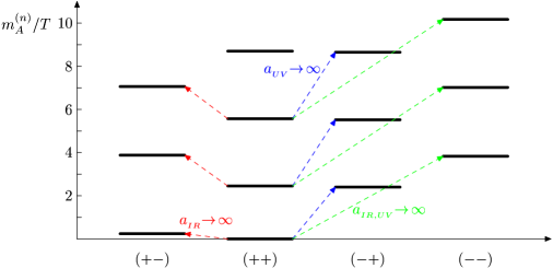
Figure 3: Kaluza-Klein masses of a bulk gauge boson in unit of $T$ when $b=a_{{}_{\rm UV}}=a_{{}_{\rm IR}}=0$.

If the SM gauge symmetry of $SU(2)_{L}\times U(1)_{Y}$ is spontaneously broken by the localized Higgs VEV, the value of $a_{\rm IR}$ becomes non-zero. Figure 4 shows, as functions of $a_{{}_{\rm IR}}$, a few lowest KK masses of a bulk gauge boson with $(++)$ parity. In the small $a_{\rm IR}$ limit, the zero mode KK mass increases gradually with $a_{{}_{\rm IR}}$. As $a_{\rm IR}$ becomes large, the rise of KK masses is saturated, eventually into the KK masses of $(+-)$ parity modes.

Figure 4: The lowest a few KK masses of a bulk gauge boson with $(++)$ parity for varying $a_{\rm IR}$. At large $a_{\rm IR}$ limit, we can easily see the masses are saturated.

When the UV brane mass parameter $a_{{}_{\rm UV}}$ turns on, however, the rise of zero mode mass with the $a_{{}_{\rm UV}}$ is not gradual even in the small $a_{{}_{\rm UV}}$ limit. To be specific, let us focus on the master equation for the $(++)$ gauge field in Eq. (14) with $a_{{}_{\rm IR}}=0$. Denoting the KK mass in unit of $T$ by $x_{A}^{(n)}\equiv{m_{A}^{(n)}}/T$, $x_{A}^{(n)}$ is the solution of

$$\frac{J_{0}({x_{A}^{(n)}})}{Y_{0}({x_{A}^{(n)}})}=\frac{-\frac{a_{{}_{\rm UV}}^{2}}{2}J_{1}(\epsilon{x_{A}^{(n)}})+\epsilon{x_{A}^{(n)}}J_{0}(\epsilon{x_{A}^{(n)}})}{-\frac{a_{{}_{\rm UV}}^{2}}{2}Y_{1}(\epsilon{x_{A}^{(n)}})+\epsilon{x_{A}^{(n)}}Y_{0}(\epsilon{x_{A}^{(n)}})}\,,$$ (20)

whose the right-handed side in the limit of $\epsilon\ll 1$ is $\left(-{1}/{4}+{1}/{a_{{}_{\rm UV}}^{2}}\right)\epsilon^{2}\,{x_{A}^{(n)}}^{2}$. In order to avoid another hierarchy in the theory, even small $a_{{}_{\rm UV}}$ is assumed larger than $\epsilon=T/k\sim 10^{-15}$. Then the right handed side of Eq. (20) is technically zero, and the $a_{{}_{\rm UV}}$-dependence disappears. As soon as the $a_{{}_{\rm UV}}$ above $10^{-15}$ turns on, the KK masses of the $(++)$ gauge field jump into those of the $(-+)$ field. In summary, the SM gauge bosons mass in the AdS₅ background can be generated either by orbifold boundary conditions or by the IR-brane localized Higgs VEV.

III Bulk fermion field without the localized mass

In 5D spacetime, the Dirac spinor is the smallest irreducible representation of the Lorentz group. Its 5D action is

$$S_{\rm fermion}=\int d^{4}xdy\sqrt{G}\left[\,\frac{i}{2}\overline{\Psi}\,\Gamma^{\underline{A}}\,e_{\underline{A}}{}^{A}\partial_{A}\Psi-\frac{i}{2}(\partial_{A}\overline{\Psi})\,\Gamma^{\underline{A}}\,e_{\underline{A}}{}^{A}+m_{D}\overline{\Psi}\Psi\right]\,,$$ (21)

where $e_{\underline{A}}{}^{A}=\mbox{diag}(e^{\sigma},e^{\sigma},e^{\sigma},e^{\sigma},1)$ is the inverse fünfbein, $\Gamma^{\underline{M}}=\left(\gamma^{\mu},\,i\gamma_{5}\right)$, $\sqrt{G}=e^{-4\sigma}$, and $\{\Gamma_{\underline{M}},\,\Gamma_{\underline{N}}\}=2\eta_{\underline{M}\,\underline{N}}=2{\rm diag}\left(+,-,-,-,-\right)$. In order to make good use of the $\mathbb{Z}_{2}\times\mathbb{Z}_{2}^{\prime}$ parity, we employ the extra dimensional coordinate $y$ in Eq. (1). With the redefinition of $\widehat{\Psi}\equiv e^{-2\sigma}\Psi$ and the relation of $\partial_{y}\Psi=e^{2\sigma}(2\sigma^{\prime}+\partial_{y})\widehat{\Psi}$, the action can be simply written by

$$S_{\rm fermion}=\int d^{4}x\,dy\left[\,\overline{\widehat{\Psi}}e^{\sigma}i\gamma^{\mu}\partial_{\mu}\widehat{\Psi}-\frac{1}{2}\overline{\widehat{\Psi}}\gamma_{5}\partial_{y}\widehat{\Psi}+\frac{1}{2}(\partial_{y}\overline{\widehat{\Psi}})\gamma_{5}\widehat{\Psi}+m_{D}\overline{\widehat{\Psi}}\widehat{\Psi}\right]\,.$$ (22)

Under the $\mathbb{Z}_{2}$ orbifold symmetry, a bulk fermion has two possible transformations of

$$\gamma_{5}\Psi_{\pm}(x,-y)\,={}\pm\Psi_{\pm}(x,y)\,.$$ (23)

To understand this $\mathbb{Z}_{2}$ symmetry more easily, we decompose the bulk fermion in terms of KK chiral fermions:

$$\widehat{\Psi}(x,y)\equiv\widehat{\Psi}_{L}+\widehat{\Psi}_{R}=\sqrt{k}\sum_{n}\left[\psi_{L}^{(n)}(z)f_{L}^{(n)}(y)+\psi_{R}^{(n)}(z)f_{R}^{(n)}(y)\right]\,.$$ (24)

When $\Psi(x,y)$ is even under $\mathbb{Z}_{2}$, for example, $f_{L}^{(n)}$ is odd while $f_{R}^{(n)}$ is even:

$$f_{L}^{(n)}(-y)=-f_{L}^{(n)}(y),\ f_{R}^{(n)}(-y)=f_{R}^{(n)}(y).$$ (25)

Similar arguments for $\mathbb{Z}_{2}^{\prime}$ symmetry can be made. Therefore, the $\mathbb{Z}_{2}\times\mathbb{Z}_{2}^{\prime}$ parity of $\Psi_{L}$ is always opposite to that of $\Psi_{R}$.

Another tricky problem arises when dealing with a bulk fermion in a finite interval. To confirm the variational principle, we separate the action into the bulk term ($S_{B}$) and the boundary term ($S_{\partial B}$):

$$S_{B}\! = \!\int\!d^{4}xdy\left[\overline{\widehat{\Psi}}_{L}e^{\sigma}i\gamma^{\mu}\partial_{\mu}\widehat{\Psi}_{L}+\overline{\widehat{\Psi}}_{R}e^{\sigma}i\gamma^{\mu}\partial_{\mu}\hat{\Psi}_{R}+m_{D}(\overline{\widehat{\Psi}}_{L}\widehat{\Psi}_{R}+\overline{\widehat{\Psi}}_{R}\widehat{\Psi}_{L})\right.$$

$$\left.-\overline{\widehat{\Psi}}_{L}\partial_{y}\widehat{\Psi}_{R}+\overline{\widehat{\Psi}}_{R}\partial_{y}\widehat{\Psi}_{L}\right],$$

$$S_{\partial B} = \int d^{4}x\,\frac{1}{2}\left[\,\overline{\widehat{\Psi}}_{L}\widehat{\Psi}_{R}-\overline{\widehat{\Psi}}_{R}\widehat{\Psi}_{L}\right]^{L}_{0}\,.$$ (27)

Since Dirac mass term in Eq. (III) is $\mathbb{Z}_{2}\times\mathbb{Z}_{2}^{\prime}$-odd, we define $m_{D}=c\,\sigma^{\prime}(y)=c\,k\mathrm{sign}(y)$. Considering both boundaries, $\sigma(y)$ is a periodic triangle wave function and thus $\mathrm{sign}(y)$ is a periodic square wave function.

With the normalization of

$$\delta_{mn}=k\int^{L}_{0}dy\,e^{\sigma}f_{L}^{(n)}f_{L}^{(m)}=k\int^{L}_{0}dy\,e^{\sigma}f_{R}^{(n)}f_{R}^{(m)}\,,$$ (28)

and the equations of motion of

$$\partial_{y}f_{R}^{(n)}-m_{D}f_{R}^{(n)} = m^{(n)}e^{\sigma}f_{L}^{(n)},$$

$$-\partial_{y}f_{L}^{(n)}-m_{D}f_{L}^{(n)} = m^{(n)}e^{\sigma}f_{R}^{(n)}\,,$$ (29)

the bulk action in Eq. (III) becomes the sum of KK fermion modes:

$$S_{\rm eff}=\int d^{4}x\sum_{n}\left[\overline{\psi}^{(n)}_{L}i\gamma^{\mu}\partial_{\mu}\psi^{(n)}_{L}+\overline{\psi}^{(n)}_{R}i\gamma^{\mu}\partial_{\mu}\psi^{(n)}_{R}-m^{(n)}(\overline{\psi}^{(n)}_{L}\psi^{(n)}_{R}+\overline{\psi}^{(n)}_{R}\psi^{(n)}_{L})\right]\ .$$ (30)

The equations of motion in the conformal coordinate $z=e^{\sigma(y)}/k$ are

$$\left(\partial_{z}+\frac{c}{z}\right)f_{L}^{(n)}=-m^{(n)}f_{R}^{(n)},\quad\left(\partial_{z}-\frac{c}{z}\right)f_{R}^{(n)}=m^{(n)}f_{L}^{(n)}\,,$$ (31)

which yield the general solutions of

$$f_{L}^{(n)}(z) = \frac{\sqrt{z}}{N_{L}^{(n)}}\left[J_{c+\frac{1}{2}}(m^{(n)}z)+\beta_{L}^{(n)}Y_{c+\frac{1}{2}}(m^{(n)}z)\right],$$

$$f_{R}^{(n)}(z) = \frac{\sqrt{z}}{N_{R}^{(n)}}\left[J_{c-\frac{1}{2}}(m^{(n)}z)+\beta_{R}^{(n)}Y_{c-\frac{1}{2}}(m^{(n)}z)\right].$$ (32)

Special properties of the Bessel function and the boundary condition lead to the following simple relations:

$$\beta_{L}^{(n)}=\beta_{R}^{(n)},\quad N_{L}^{(n)}=-N_{R}^{(n)}\,.$$ (33)

This is because either $f_{L}^{(n)}$ or $f_{R}^{(n)}$ is an continuous odd function which vanishes at the boundary. For example, consider the case where $f_{R}^{(n)}$ is odd. With Eq. (31), we have

$$\left.f^{(n)}_{R}\right|_{z=\frac{1}{k}}=0,$$ (34)

$$\left.\left(\partial_{z}+\frac{c}{z}\right)f^{(n)}_{L}\right|_{z=\frac{1}{k}}=0.$$ (35)

Equation (34) leads to $\beta_{R}^{(n)}=-{J_{c-\frac{1}{2}}(\frac{m^{(n)}}{k})}/{Y_{c-\frac{1}{2}}(\frac{m^{(n)}}{k})}$. Due to the Bessel function relation of

$$\left(\partial_{z}+\frac{c}{z}\right)f_{L}^{(n)}(z) = \frac{m^{(n)}\sqrt{z}}{N_{L}^{(n)}}\left[J_{c-\frac{1}{2}}(m^{(n)}z)+\beta_{L}^{(n)}Y_{c-\frac{1}{2}}(m^{(n)}z)\right],$$ (36)

$$\left(\partial_{z}-\frac{c}{z}\right)f_{R}^{(n)}(z) = -\frac{m^{(n)}\sqrt{z}}{N_{R}^{(n)}}\left[J_{c+\frac{1}{2}}(m^{(n)}z)+\beta_{R}^{(n)}Y_{c+\frac{1}{2}}(m^{(n)}z)\right]\,,$$

Eq. (35) yields

$$\beta_{L}^{(n)}=-\frac{J_{c-\frac{1}{2}}(\frac{m^{(n)}}{k})}{Y_{c-\frac{1}{2}}(\frac{m^{(n)}}{k})}=\beta_{R}^{(n)}.$$ (37)

It is clear that $N_{L}^{(n)}=-N_{R}^{(n)}$ from Eq. (36).

Without the localized fermion mass, KK masses of a bulk fermion depend on its $\mathbb{Z}_{2}\times\mathbb{Z}_{2}^{\prime}$ parity and the bulk Dirac mass parameter $c$. Under the $\mathbb{Z}_{2}\times\mathbb{Z}_{2}^{\prime}$ symmetry, a generic 5D bulk fermion can have the following four different transformation property:

$$\hat{\Psi}_{1}(x,y) = \sqrt{k}\sum_{n}[\psi^{(n)}_{1L}(x)f^{(n)}_{1L(++)}(y)+\psi^{(n)}_{1R}(x)f^{(n)}_{1R(--)}(y)]\,,$$ (38)

$$\hat{\Psi}_{2}(x,y) = \sqrt{k}\sum_{n}[\psi^{(n)}_{2L}(x)f^{(n)}_{2L(--)}(y)+\psi^{(n)}_{2R}(x)f^{(n)}_{2R(++)}(y)]\,,$$ (39)

$$\hat{\Psi}_{3}(x,y) = \sqrt{k}\sum_{n}[\psi^{(n)}_{3L}(x)f^{(n)}_{3L(+-)}(y)+\psi^{(n)}_{3R}(x)f^{(n)}_{3R(-+)}(y)]\,,$$ (40)

$$\hat{\Psi}_{4}(x,y) = \sqrt{k}\sum_{n}[\psi^{(n)}_{4L}(x)f^{(n)}_{4L(-+)}(y)+\psi^{(n)}_{4R}(x)f^{(n)}_{4R(+-)}(y)]\,,$$ (41)

where the $\mathbb{Z}_{2}\times\mathbb{Z}_{2}^{\prime}$ parities are denoted by $(PP^{\prime})$ in $f^{(n)}_{(PP^{\prime})}$. Note that the $P\,(P^{\prime})$ of $f_{iL}^{(n)}$ is opposite to that of $f_{iR}^{(n)}$.

With Eq. (33), the mode functions are

$$f_{iL}^{(n)}(z) = \frac{\sqrt{z}}{N_{i}^{(n)}}\left[J_{c_{i}+1/2}(m_{i}^{(n)}z)+\beta_{i}^{(n)}Y_{c_{i}+1/2}(m_{i}^{(n)}z)\right],$$

$$f_{iR}^{(n)}(z) = -\frac{\sqrt{z}}{N_{i}^{(n)}}\left[J_{c_{i}-1/2}(m_{i}^{(n)}z)+\beta_{i}^{(n)}Y_{c_{i}-1/2}(m_{i}^{(n)}z)\right]\,.$$ (42)

The coefficient $\beta_{i}^{(n)}$ is fixed by the fact that a $\mathbb{Z}_{2}\,(\mathbb{Z}_{2}^{\prime})$-odd function vanishes at the corresponding boundary. For example, the $f_{1R(--)}^{(n)}$ and $f_{2L(--)}$ vanish at both UV and IR branes, which doubly constrain the $\beta_{i}^{(n)}$:

$$\beta_{1}^{(n)} = -\dfrac{J_{c_{1}-1/2}(m^{(n)}/k)}{Y_{c_{1}-1/2}(m^{(n)}/k)}=-\dfrac{J_{c_{1}-1/2}(m^{(n)}/T)}{Y_{c_{1}-1/2}(m^{(n)}/T)}\,,$$ (43)

$$\beta_{2}^{(n)} = -\dfrac{J_{c_{2}+1/2}(m^{(n)}/k)}{Y_{c_{2}+1/2}(m^{(n)}/k)}=-\dfrac{J_{c_{2}+1/2}(m^{(n)}/T)}{Y_{c_{2}+1/2}(m^{(n)}/T)}\,.$$ (44)

Similarly we have

$$\beta_{3}^{(n)} = -\dfrac{J_{c_{3}-1/2}(m^{(n)}/k)}{Y_{c_{3}-1/2}(m^{(n)}/k)}=-\dfrac{J_{c_{3}+1/2}(m^{(n)}/T)}{Y_{c_{3}+1/2}(m^{(n)}/T)}\,,$$ (45)

$$\beta_{4}^{(n)} = -\dfrac{J_{c_{4}+1/2}(m^{(n)}/k)}{Y_{c_{4}+1/2}(m^{(n)}/k)}=-\dfrac{J_{c_{4}-1/2}(m^{(n)}/T)}{Y_{c_{4}-1/2}(m^{(n)}/T)}\,.$$ (46)

Figure 5: KK mass spectra of a bulk fermion $\Psi_{i}$ in unit of $T$ as a function of the bulk mass parameter $c$. The $\mathbb{Z}_{2}\times\mathbb{Z}_{2}^{\prime}$ parities of each fermion is described in the text.

In Fig. 5, we present the KK masses of a bulk fermion $\Psi_{i}$ in unit of $T$ as a function of the bulk mass parameter $c$. It is clear that $\Psi_{1}(\supset\Psi_{1L}^{(++)})$ and $\Psi_{2}(\supset\Psi_{2R}^{(++)})$ can accommodate zero modes. An unexpected feature is that the zero mode mass of $\Psi_{3}$ ($\Psi_{4}$) can be considerably light for $c_{3}>0.5~{}(c_{4}<-0.5)$.

IV Bulk fermion with Yukawa interaction on the brane

The accommodation of the SM fermions in the bulk RS theories has some delicate features. First a single SM fermion with left- and right-handed chirality should be described by two 5D Dirac fermions. For example, the left-handed up quark is to be described by the $\Psi_{1}$ type while the right-handed up quark by the $\Psi_{2}$ type. Another interesting problem is the generation of light and realistic masses for the SM fermions Gherghetta:2000qt . Even though the KK zero modes are good candidates for the SM fermions, their zero masses should be lifted only a little. In the ADMS model, the localized Higgs VEV plays this role without explicit breaking of gauge symmetry Agashe:2003zs . Different strengths of Yukawa couplings can explain diverse mass spectrum of the SM fermions as in the SM. In the Higgsless model, it is also possible to get realistic SM fermion masses by boundary conditions Csaki:2003sh . Unfortunately the basic set-up is somewhat complicated for each SM fermion: A 4D gauge invariant Dirac mass is to be introduced, which is localized on the IR brane and mixes the $\Psi_{1}$ and $\Psi_{2}$ types; a new 4D Dirac spinor, localized on the UV brane, is also required to mix with the $\Psi_{2}$ type fermion.

For simplicity, we consider the case where SM fermion masses are generated by the localized Yukawa couplings between two fermion fields of $\Psi_{1}$ and $\Psi_{2}$. The five-dimensional fermion action is

$$S_{\rm fermion}=\int d^{4}x\int^{L}_{0}dy\left[\overline{\widehat{\Psi}}_{i}e^{\sigma}i\gamma^{\mu}\partial_{\mu}\widehat{\Psi}_{i}-\frac{1}{2}\overline{\widehat{\Psi}}_{i}\gamma_{5}\partial_{y}\widehat{\Psi}_{i}+\frac{1}{2}(\partial_{y}\overline{\widehat{\Psi}}_{i})\gamma_{5}\widehat{\Psi}_{i}+m_{iD}\overline{\widehat{\Psi}}_{i}\widehat{\Psi}_{i}\right],$$ (47)

where $\sum_{i=1}^{2}$ is assumed for repeated index $i$. The Yukawa interaction localized on the IR brane couples the $\Psi_{1}$ with $\Psi_{2}$:

$$S_{\rm Yukawa}=-\int d^{4}x\,dy\lambda_{v}\left(\overline{\hat{\Psi}}_{1}\hat{\Psi}_{2}+\overline{\hat{\Psi}}_{2}\hat{\Psi}_{1}\right)\delta(y-L).$$ (48)

Here, $\lambda_{v}\equiv\lambda_{5}\langle H\rangle/T$, $\lambda_{5}$ is the 5D dimensionless Yukawa coupling and $H(x)$ is a canonically normalized Higgs scalar defined by $H(x)=\epsilon H_{5}(x)$. The 5D total action becomes $S_{5D}=S_{\rm fermion}+S_{\rm Yukawa}$.

To simplify $S_{5D}$, a technical problem arises as the Dirac delta function is positioned at $y=L$ while the $y$-integration range is in $[0,L]$ Csaki:2003sh . We regulate this by using the periodicity of $S^{1}$ space and dividing the integration into

$$S_{5D}=\int^{L-\varepsilon}_{0}dy\ S_{4D}+\frac{1}{2}\int^{L+\varepsilon}_{L-\varepsilon}dy\ S_{4D}\equiv S_{\rm bulk}+S_{\partial}.$$ (49)

For a small positive $\varepsilon$, $S_{\rm bulk}$ is well-defined, given by

$$S_{\rm bulk} = \int d^{4}x\left\{\int^{L-\varepsilon}_{0}dy\,\left[\overline{\widehat{\Psi}}_{i}\left(e^{\sigma}i\gamma^{\mu}\partial_{\mu}-\gamma_{5}\partial_{y}+m_{iD}\right)\widehat{\Psi}_{i}\right]+\left.\frac{1}{2}\overline{\widehat{\Psi}}_{i}\gamma_{5}\widehat{\Psi}_{i}\right|^{L-\varepsilon}_{0}\right\}\,,$$ (50)

where $f(x)|_{a}^{b}\equiv f(b)-f(a)$ and $S_{\partial}$ is

$$S_{\partial}=\int d^{4}x\left\{-\frac{1}{2}\int^{L+\varepsilon}_{L-\varepsilon}dy\,\overline{\widehat{\Psi}}_{i}\gamma_{5}\partial_{y}\widehat{\Psi}_{i}-\frac{1}{2}\,\lambda_{v}\left.\left(\overline{\widehat{\Psi}}_{1}\widehat{\Psi}_{2}+\overline{\widehat{\Psi}}_{2}\widehat{\Psi}_{1}\right)\right|_{y=L}+\left.\frac{1}{4}\,\overline{\widehat{\Psi}}_{i}\gamma_{5}\widehat{\Psi}_{i}\right|^{L+\varepsilon}_{L-\varepsilon}\right\}\,.$$ (51)

The absence of the localized fermion mass on the Planck brane guarantees the continuity of the mode functions at $y=0$:

$$\left.\overline{\widehat{\Psi}}_{i}\gamma_{5}\widehat{\Psi}_{i}\right|_{y=0}=0\,.$$ (52)

Furthermore the $\mathbb{Z}_{2}^{\prime}$-oddity of $\overline{\widehat{\Psi}}_{i}\gamma_{5}\widehat{\Psi}_{i}$ implies

$$\left.\overline{\widehat{\Psi}}_{i}\gamma_{5}\widehat{\Psi}_{i}\right|^{L+\varepsilon}_{L-\varepsilon}=\left.-2\,\overline{\widehat{\Psi}}_{i}\gamma_{5}\widehat{\Psi}_{i}\right|_{y=L-\varepsilon}\,.$$ (53)

Equations (52) and (53) give rise to the cancelation between the last terms of Eqs. (50) and (51). Therefore, the $S_{\rm bulk}$ is

$$S_{\rm bulk} = \int\!d^{4}x\!\int^{L-\varepsilon}_{0}dy\left[e^{\sigma}(\overline{\widehat{\Psi}}_{iL}i\gamma^{\mu}\partial_{\mu}\widehat{\Psi}_{iL}+\overline{\widehat{\Psi}}_{iR}i\gamma^{\mu}\partial_{\mu}\widehat{\Psi}_{iR})\right.$$

$$\left.-\overline{\widehat{\Psi}}_{iL}(\partial_{y}-m_{iD})\widehat{\Psi}_{iR}+\overline{\widehat{\Psi}}_{iR}(\partial_{y}+m_{iD})\widehat{\Psi}_{iL}\right]\,.$$

More comments on simplifying $S_{\partial}$ are in order here. The $\mathbb{Z}_{2}^{\prime}$-even parity of $\widehat{\Psi}_{1L}$ and $\widehat{\Psi}_{2R}$ guarantees the continuity at $y=L$, which eliminates the infinitesimal integration of $\overline{\widehat{\Psi}}_{1R}\gamma_{5}\partial_{y}\widehat{\Psi}_{1L}$ and $\overline{\widehat{\Psi}}_{2L}\gamma_{5}\partial_{y}\widehat{\Psi}_{2R}$ in Eq. (51). On the contrary, the presence of Yukawa term hints the discontinuity of $\mathbb{Z}_{2}^{\prime}$-odd $\widehat{\Psi}_{1R}$ and $\widehat{\Psi}_{2L}$ at $y=L$. Nevertheless at $y=L$ the values of $\mathbb{Z}_{2}^{\prime}$-odd functions can be assigned zero, which is possible by setting zero the $y=L$ boundary value of periodic $\mathrm{sign}(y)$ function in the bulk Dirac mass term . Among Yukawa terms in Eq. (51), therefore, $(\overline{\widehat{\Psi}}_{1R}\widehat{\Psi}_{2L}+h.c.)|_{y=L}$ vanishes. Finally integration by part and Eq. (53) simplifies $S_{\partial}$ as

$$S_{\partial} = \int d^{4}x\left[\,\left.\left(\overline{\widehat{\Psi}}_{1L}\widehat{\Psi}_{1R}-\overline{\widehat{\Psi}}_{2L}\widehat{\Psi}_{2R}\right)\right|_{y=L-\varepsilon}-\frac{\lambda_{v}}{2}\left.\left(\overline{\widehat{\Psi}}_{1L}\widehat{\Psi}_{2R}+\overline{\widehat{\Psi}}_{2R}\widehat{\Psi}_{1L}\right)\right|_{y=L}\right]\,.$$ (55)

The variation of $S_{\rm bulk}$ gives equations of motion for bulk fermions, while $S_{\partial}=0$ gives boundary conditions.

Without Yukawa terms, $\Psi_{1}$ and $\Psi_{2}$ have their own KK mass spectra, determined by the bulk Dirac mass parameter $c_{i}$. As the Yukawa couplings turn on between $\Psi_{1}$ and $\Psi_{2}$, $\psi_{1L}^{(n)}$ and $\psi_{1R}^{(n)}$ mix with $\psi_{2L}^{(n)}$ and $\psi_{2R}^{(n)}$, respectively. Denoting the KK mass eigenstates by $\chi^{{(n)}}_{L,R}(y)$, the KK expansion of the bulk field is

$$\hat{\Psi}_{i}=\sqrt{k}\sum_{n}\left[\chi_{L}^{(n)}(x)f_{iL}^{(n)}(y)+\chi_{R}^{(n)}(x)f_{iR}^{(n)}(y)\right].$$ (56)

With the modified normalization of

$$\sum_{i=1,2}k\int_{0}^{L}dy\,e^{\sigma}{f}^{(n)}_{iL}{f}^{(m)}_{iL}=k\sum_{i=1,2}\int_{0}^{L}dy\,e^{\sigma}{f}^{(n)}_{iR}{f}^{(m)}_{iR}=\delta_{nm}\,,$$ (57)

and the equations of motion of

$$\partial_{y}f_{iR}^{(n)}-m_{iD}f_{iR}^{(n)} = m^{(n)}e^{\sigma}f_{iL}^{(n)}\,,$$

$$-\partial_{y}f_{iL}^{(n)}-m_{iD}f_{iL}^{(n)} = m^{(n)}e^{\sigma}f_{iR}^{(n)},$$ (58)

the 4D effective action consists of the KK fermions:

$$S_{\rm eff}=\int d^{4}x\sum_{n}\left[\overline{\chi}^{(n)}_{L}i\gamma^{\mu}\partial_{\mu}\chi^{(n)}_{L}+\overline{\chi}^{(n)}_{R}i\gamma^{\mu}\partial_{\mu}\chi^{(n)}_{R}-m^{(n)}(\overline{\chi}^{(n)}_{L}\chi^{(n)}_{R}+\overline{\chi}^{(n)}_{R}\chi^{(n)}_{L})\right]\ .$$ (59)

The general solutions of Eq. (IV) are the same as Eq. (42).

The substitution of Eq. (56) into $S_{\partial}=0$ with the continuity of $\mathbb{Z}_{2}^{\prime}$-even functions at $y=L$, we have

$$f_{1R}^{(n)}|_{y=L-\varepsilon}=\frac{\lambda_{v}}{2}f_{2R}^{(n)}|_{y=L}\,,\quad f_{2L}^{(n)}|_{y=L-\varepsilon}=-\frac{\lambda_{v}}{2}f_{1L}^{(n)}|_{y=L}.$$ (60)

In the followings, we will ignore infinitesimal $\varepsilon$ and consider only $z$ coordinates. Finally we have all boundary conditions at $z_{{}_{\rm UV}}=1/k$ and $z_{{}_{\rm IR}}=1/T$:

$$\left.f_{1R}^{(n)}\right|_{\frac{1}{k}}=0, \left.f_{1R}^{(n)}\right|_{\frac{1}{T}}=\left.\frac{\lambda_{v}}{2}f_{2R}^{(n)}\right|_{\frac{1}{T}},$$ (61)

$$\left.f_{2L}^{(n)}\right|_{\frac{1}{k}}=0, \left.f_{2L}^{(n)}\right|_{\frac{1}{T}}=-\left.\frac{\lambda_{v}}{2}f_{1L}^{(n)}\right|_{\frac{1}{T}},$$ (62)

$$\left.(\partial_{z}+\frac{c_{1}}{z})f_{1L}^{(n)}\right|_{\frac{1}{k}}=0, \left.(\partial_{z}+\frac{c_{1}}{z})f_{1L}^{(n)}\right|_{\frac{1}{T}}=\left.\frac{\lambda_{v}}{2}m^{(n)}f_{2R}^{(n)}\right|_{\frac{1}{T}},$$ (63)

$$\left.(\partial_{z}-\frac{c_{2}}{z})f_{2R}^{(n)}\right|_{\frac{1}{k}}=0, \left.(\partial_{z}-\frac{c_{2}}{z})f_{2R}^{(n)}\right|_{\frac{1}{T}}=\left.\frac{\lambda_{v}}{2}m^{(n)}f_{1L}^{(n)}\right|_{\frac{1}{T}}.$$ (64)

At $z=1/k$ the relations are the same as the case of $\lambda_{v}=0$, yielding

$$\beta_{1}^{(n)}\equiv\beta_{1R}^{(n)} = \beta_{1L}^{(n)}=-\frac{J_{c_{1}-\frac{1}{2}}(\frac{m^{(n)}}{k})}{Y_{c_{1}-\frac{1}{2}}(\frac{m^{(n)}}{k})},$$ (65)

$$\beta_{2}^{(n)}\equiv\beta_{2L}^{(n)} = \beta_{2R}^{(n)}=-\frac{J_{c_{2}+\frac{1}{2}}(\frac{m^{(n)}}{k})}{Y_{c_{2}+\frac{1}{2}}(\frac{m^{(n)}}{k})}.$$

As in the previous section, the normalization factors of the left-handed and right-handed mode functions are related by

$$N_{1}^{(n)}\equiv N_{1L}^{(n)}=-N_{1R}^{(n)},\quad N_{2}^{(n)}\equiv-N_{2L}^{(n)}=N_{2R}^{(n)}\,.$$ (66)

The boundary conditions at $z=1/T$ in Eqs. (61) and (62) give

$$\frac{1}{N_{1}^{(n)}}\left[J_{c_{1}-\frac{1}{2}}(x^{(n)})+\beta_{1}^{(n)}Y_{c_{1}-\frac{1}{2}}(x^{(n)})\right] = -\frac{\lambda_{v}}{2N_{2}^{(n)}}\left[J_{c_{2}-\frac{1}{2}}(x^{(n)})+\beta_{2}^{(n)}Y_{c_{2}-\frac{1}{2}}(x^{(n)})\right]\,,$$ (67)

$$\frac{1}{N_{2}^{(n)}}\left[J_{c_{2}+\frac{1}{2}}(x^{(n)})+\beta_{2}^{(n)}Y_{c_{2}+\frac{1}{2}}(x^{(n)})\right] = \phantom{-}\frac{\lambda_{v}}{2N_{1}^{(n)}}\left[J_{c_{1}+\frac{1}{2}}(x^{(n)})+\beta_{1}^{(n)}Y_{c_{1}+\frac{1}{2}}(x^{(n)})\right]\,,$$ (68)

where $x^{(n)}=m^{(n)}/T$. The elimination of $N_{1}^{(n)}$ and $N_{2}^{(n)}$ by multiplying Eq. (67) and Eq. (68) and the substitution of $\beta_{1,2}^{(n)}$ in Eq. (65) produce the final master equation:

$${\cal J}^{--}_{1}(x^{(n)}){\cal J}^{++}_{2}(x^{(n)})=-\frac{\lambda_{v}^{2}}{4}{\cal J}^{-+}_{1}(x^{(n)}){\cal J}^{+-}_{2}(x^{(n)}),$$ (69)

where ${\cal J}^{\pm\pm^{\prime}}_{i}$ is defined by

$${\cal J}^{\pm\pm^{\prime}}_{i}(x^{(n)}) = Y_{c_{i}\pm\frac{1}{2}}\left(\epsilon\,x^{(n)}\right)J_{c_{i}\pm^{\prime}\frac{1}{2}}\left(x^{(n)}\right)-J_{c_{i}\pm\frac{1}{2}}\left(\epsilon\,x^{(n)}\right)Y_{c_{i}\pm^{\prime}\frac{1}{2}}\left(x^{(n)}\right)\,.$$ (70)

These master equations clearly show the relation of the $\mathbb{Z}_{2}\times\mathbb{Z}_{2}^{\prime}$ parity and the large localized Higgs VEV as in the gauge boson case. When $\lambda_{v}$ is zero, the KK spectra of $\hat{\Psi}_{1}$ and $\hat{\Psi}_{2}$ are the same as in the previous section. As $\lambda_{v}\rightarrow\infty$ the right-handed side of Eq. (68) should vanish, yielding

$$\beta_{1}^{(n)}|_{\lambda_{v}\to\infty}=-\frac{J_{c_{1}+1/2}(m^{(n)}/T)}{Y_{c_{1}+1/2}(m^{(n)}/T)}=-\frac{J_{c_{1}-1/2}(m^{(n)}/k)}{Y_{c_{1}-1/2}(m^{(n)}/k)}\,,$$ (71)

where the second equality comes from Eq. (65). This is identical to the $\beta^{(n)}_{3}$ in Eq. (45) except for $c_{i}$. The KK mass spectrum of $\Psi_{1}$ in the large $\lambda_{v}$ limit is the same as that of $\Psi_{3}$ without $\lambda_{v}$: $\Psi_{1}$ mimics $\Psi_{3}$. Similarly, the $\Psi_{2}$ mimics $\Psi_{4}$.

Figure 6: KK mass spectra of bulk fermions $\Psi_{1}(\supset\Psi_{1L}^{(++)})$ and $\Psi_{2}(\supset\Psi_{2R}^{(++)})$ in unit of $T$ as a function of Yukawa mass term $\lambda_{v}$.

Figure 6 shows the KK masses of $\Psi_{1}$ and $\Psi_{2}$ as a function of $\lambda_{v}$. We present the numerical results for two cases, $[c_{1}=0.4,c_{2}=-0.4]$ case and $[c_{1}=0.4,c_{2}=0.4]$ case. As the Yukawa term increases, the zero mode acquires non-zero mass $m^{(0)}$. For large $\lambda_{v}$, the $m^{(0)}$ becomes saturated as in the gauge boson case, since the KK mode become a mixed state of higher KK modes. Another interesting feature is that the first KK mode mass decreases as $\lambda_{v}$ increases, contrary to the bulk gauge boson case where $m_{A}^{(1)}$ increases with $a_{{}_{\rm IR}}$ (see Fig. 4). The mass drop due to $\lambda_{v}$ is maximal when the two KK mass spectra were degenerate at $\lambda_{v}=0$, e.g., $[c_{1}=0.4,c_{2}=-0.4]$ case. This KK mode degenerate case will leave dramatic signatures at high energy colliders: The KK modes of light quarks show doubly degenerate mass spectrum while the first KK mode of top quark can be considerably light. It is very feasible, therefore, that the first signal of KK fermions comes from the top quark mode which alone possesses non-negligible Yukawa mass. The saturation of zero mode mass and the dropping of first excited KK mode mass are consistent with the existence of two light KK mode in the transition from $\hat{\Psi}_{1}$ to $\hat{\Psi}_{3}$ and $\hat{\Psi}_{2}$ to $\hat{\Psi}_{4}$ spectra for the $\lambda_{v}\rightarrow\infty$ limit.

V Gauge coupling universality

In the previous sections, it is shown that the presence of the localized mass terms generates non-zero masses for the zero modes as well as modifying other higher KK mode masses. Another important influence of localized mass terms is on mode functions. Without localized mass terms, the zero mode functions of a bulk gauge boson ($\tilde{f}_{A}^{(0)}$) and a $\Psi_{1}$-type fermion ($\tilde{f}_{L,R}^{(0)}$) are

$$\tilde{f}_{A}^{(0)} = \frac{1}{\sqrt{kL}},$$ (72)

$$\tilde{f}_{L(++)}^{(0)} = \frac{(kz)^{-c}}{N^{(0)}}\,,\quad\tilde{f}_{R(--)}^{(0)}=0,$$

where the tildes over mode functions emphasize the absence of boundary mass terms. The localized masses change these functional forms. Since our four-dimensional effective gauge coupling is obtained by convoluting mode functions of a gauge boson and two fermions, different changes of mode functions by different localized masses can deviate the SM relations of gauge couplings. In what follows, we focus on a simple scenario where only the top quark Yukawa coupling is non-zero. If the 4D gauge coupling $g$ is defined by the $u$-$d$-$W$ coupling, the top-bottom-$W$ coupling, $g_{Wtb}$, departs from $g$ due to the deformed mode functions: The gauge coupling universality may be in danger.

In the five dimensional RS theory, the changed current interaction of $SU(2)_{L}$ is

$$S_{CC}=\int d^{4}x\int dz\frac{ig_{5}}{\sqrt{2k}}\,\overline{\hat{q}}_{u}(x,z){\hbox to0.0pt{/\hss}W}^{+}(x,z)\hat{q}_{d}(x,z)+H.c.,$$ (73)

where $g_{5}$ is the dimensionless 5D gauge coupling, $Q=(q_{u},q_{d})^{T}$ is a $SU(2)_{L}$ doublet. The $q_{u}(x,y)$ and $q_{d}(x,y)$ are $\Psi_{1}$ type in Eq. (38), i.e., $q_{uL}$ and $q_{dL}$ have $(++)$ parity. The five dimensional gauge coupling $g_{5}$ is related with four dimensional gauge coupling $g$ by

$$g\equiv g_{5}\int kdzf_{q_{u}L}^{(0)}f_{q_{d}L}^{(0)}{f}_{W}^{(0)}\,.$$ (74)

If the localized gauge boson mass is absent so that $\tilde{f}_{W}^{(0)}$ is constant, the fermion mode function normalization in Eq. (28) guarantees the same gauge coupling strength, irrespective of the localized Yukawa coupling strength. Gauge coupling universality remains intact.

As the localized gauge mass terms turn on, non-constant $f_{W}^{(0)}$ leads to different relations between $g$ and $g_{5}$ according to $\lambda_{v}$. We define the four-dimensional gauge coupling $g$ by the $W$-$u$-$d$ coupling with the up and down quark Yukawa couplings neglected:

$$g\equiv g_{5}\int kdz\tilde{f}_{q_{u}L}^{(0)}\tilde{f}_{q_{d}L}^{(0)}f_{W}^{(0)}\,.$$ (75)

Substantial top quark Yukawa coupling $\lambda_{t}$ changes the mode function $f_{tL}^{(0)}$ and thus the $W$-$t$-$b$ gauge coupling ${g_{{}_{Wtb}}}$. Note that the assumption of $\lambda_{b}=0$ leads to $\tilde{f}_{bR}^{(0)}=0$, eliminating anomalous right-handed $Wtb$ coupling. The degree of gauge coupling universality violation is defined by

$$\delta g_{Wtb}=\frac{g_{Wtb}}{g}-1=\frac{\int kdz{f}_{q_{t}L}^{(0)}\tilde{f}_{q_{b}L}^{(0)}f_{W}^{(0)}}{\int kdz\tilde{f}_{q_{u}L}^{(0)}\tilde{f}_{q_{d}L}^{(0)}f_{W}^{(0)}}-1\,.$$ (76)

For the numerical evaluation of $\delta g_{Wtb}$, let us discuss the model parameters. First we have the effective electroweak scale $T$. Since the up and down quarks in a given $SU(2)_{L}$ doublet should shared the same bulk Dirac mass, we have two bulk Dirac mass parameter for the first and third generation, denoted by $c$ and $c_{t}$. Non-zero $a_{{}_{\rm IR}}$ and $\lambda_{t}$ are traded with the observed $m_{W}$ and $m_{\rm top}$. In summary, the following three parameters determine $\delta g_{Wtb}$:

$$T,\quad c,\quad c_{t}\,.$$ (77)

Figure 7 shows the $\delta g_{Wtb}$ as a function of $T$. It can be easily seen that the deviation decreases with increasing $t$, and is negligible unless $c$ is not too different from $c_{t}$. In particular, the $c=c_{t}$ case practically preserves the gauge coupling universality. However, if $|c-c_{t}|$ becomes substantial (e.g., $[c=-c_{t}=0.4]$ case), the deviation can be a few percent for $T\simeq 1.5\mathrm{TeV}$. Concerning the KK mass spectra, the $c\approx-c_{t}$ case allows substantially light KK mass of the first KK mode as $\lambda_{v}$ increases. On the contrary, the $c\approx c_{t}$ case implies almost negligible $\delta g_{Wtb}$ even for relative light $T$ whose KK mass spectra are quite different for $\Psi_{1}$ and $\Psi_{2}$. In conclusions, the parameter space which guarantees gauge coupling universality has the KK mass spectrum which is similar with the KK masses without Yukawa terms.

Figure 7: The degree of the gauge coupling non-universality, defined by $\delta g_{Wtb}=g_{Wtb}/g-1$, as a function of $T$ for various combinations of $c$ and $c_{t}$.

Even though the violation of gauge coupling unification is, if any, a breakthrough in particle physics, its magnitude with $T$ around a few TeV is below a few percent. At a hadron collider like LHC, it is too small to detect. If its correlation with other physical observable such as KK masses is strong enough, it can be a valuable information. Restricting ourselves to the KK mode degenerate case (i.e., $c_{qL}=-c_{qR}$), we plot the correlation between $\delta g_{Wtb}$ and the mass difference of the first KK modes of light quark and top quark in unit of their mass sum in Fig. 8. The effective electroweak scale $T$ is fixed to be 2 TeV, while the parameter space of $c$ and $c_{T}$ in $[-0.4,\,0.4]$ are all scanned. The parameters $\lambda_{v}$ and $a_{{}_{\rm IR}}$ are determined by the SM top quark and $W$ boson mass, respectively. As can be seen in Fig. 8, we do have quite significant correlation. In the parameter space where the first KK mode of top quark is lighter than that of light quarks, $\delta g_{Wtb}$ is negative.

Figure 8: In the KK mode degenerate case, we plot the correlation between the $\delta g_{Wtb}=g_{Wtb}/g-1$ and the mass difference of the first KK modes of light quark and top quark. The effective electroweak scale $T$ is fixed to be 2 TeV, and $c,~{}c_{T}\in[-0.4,\,0.4]$.

VI Conclusion

We have studied master equations for the Kaluza-Klein (KK) masses of a bulk gauge boson and a bulk fermion in a five-dimensional (5D) warped space compactified on a $S^{1}/\mathbb{Z}_{2}\times\mathbb{Z}_{2}^{\prime}$ orbifold. These master equations accommodate the general case with the brane-localized and bulk mass terms. Comprehensive understanding for the KK mass spectra and their behavior is crucial to verify and discriminate the Higgsless model from the ADMS model.

After presenting master equations for the bulk gauge boson, it is explicitly shown that the Neumann boundary condition (for $\mathbb{Z}_{2}$-even parity) in the limit of large localized mass is equivalent to the Dirichlet boundary condition (for $\mathbb{Z}_{2}$-odd parity). This correspondence relates among KK mass spectra of gauge bosons with different $\mathbb{Z}_{2}\times\mathbb{Z}_{2}^{\prime}$ parities. A bulk gauge boson with $(++)$ parity and very large localized mass on the UV brane (denoted by $a_{{}_{\rm UV}}$) has the same KK mass spectrum with a $(-+)$ bulk gauge boson without any localized mass. In brief, the $(++)$ gauge field in the large $a_{{}_{\rm UV}}$ limit mimics $(-+)$ gauge field. Similarly, a $(++)$ bulk gauge boson in the large $a_{{}_{\rm IR}}$ limit mimics a $(+-)$ bulk gauge boson without any localized mass. This implies that the ADMS model in the large limit of the Higgs VEV can be related to the Higgsless model. Thus we can understand why one cannot avoid TeV-scaled KK states even in the case of infinite VEV of the localized Higgs boson(s). This is a generic property of the gauge theory in the truncated AdS space with TeV-valued boundary. Through numerical calculations, we have presented the KK masses of a bulk gauge boson for various $\mathbb{Z}_{2}\times\mathbb{Z}_{2}^{\prime}$ parities. The first KK mode with $(+-)$ parity is shown to be remarkably light with mass of order 100 GeV. The $a_{{}_{\rm IR}}$-dependence of the KK masses for $(++)$ parity is also presented: With increasing $a_{{}_{\rm IR}}$, not only does the zero mode KK mass acquire non-zero mass, but the first KK mass also increase. We have also shown that the method of $a_{{}_{\rm UV}}$ to raise the zero mode mass is different: As soon as the $a_{{}_{\rm UV}}$ above $\sim 10^{-15}$, the zero mode mass jumps to the TeV scale.

We have extended this discussion to the bulk fermion case. A bulk fermion on a $S^{1}/\mathbb{Z}_{2}\times\mathbb{Z}_{2}^{\prime}$ orbifold has four different boundary parities: The parity of the left-handed chiral fermion can be $(++)$, $(+-)$, $(-+)$, and $(--)$, while the parity of the corresponding right-handed fermion is opposite. First we have considered a simple case without any localized mass term. Through numerical calculations, it was shown that the first KK mode mass of $\Psi_{3}\supset\Psi_{3L}^{(+-)}$ and $\Psi_{4}\supset\Psi_{4L}^{(-+)}$ is substantially light for $c_{3}>0.5$ and $c_{4}<-0.5$, respectively. In order to explain the SM fermion masses, we have introduced the brane localized Yukawa coupling between $\Psi_{1}\supset\Psi_{1L}^{(++)}$ and $\Psi_{2}\supset\Psi_{2R}^{(++)}$. From the coupled boundary conditions, the final master equations are derived for the KK masses of bulk fermions. Similar correspondence between the $\mathbb{Z}_{2}\times\mathbb{Z}_{2}^{\prime}$ parity and the large localized Yukawa coupling is also shown: The $\Psi_{1}$ ($\Psi_{2}$) as $\lambda_{v}\to\infty$ mimics the $\Psi_{3}$ ($\Psi_{4}$) with $\lambda_{v}=0$. Another interesting feature is that the first KK mode mass decreases with increasing Yukawa coupling. In the future collider, the top quark KK mode is one of the first candidates to be detected.

Finally we have investigated the violation of gauge coupling universality, $\delta g_{Wtb}$, in a simple scenario where only the top quark Yukawa coupling is considered. This occurs as the non-zero localized masses deviate mode functions. Numerical calculation shows, however, that the violation degree is not severe in mode parameter space. Restricted in the KK mode degenerate case, we have demonstrated quite significant correlation between $\delta g_{Wtb}$ and the first KK mass of top quark with respect to light quark KK mass.

References

(1)
S. Weinberg,
Phys. Rev. D 13, 974 (1976);
Phys. Rev. D 19, 1277 (1979);
L. Susskind,
Phys. Rev. D 20, 2619 (1979).
(2)
J. M. Maldacena,
Adv. Theor. Math. Phys. 2, 231 (1998) [Int. J. Theor. Phys. 38, 1113 (1999)] [arXiv:hep-th/9711200].
(3)
S. S. Gubser, I. R. Klebanov and A. M. Polyakov,
Phys. Lett. B 428, 105 (1998) [arXiv:hep-th/9802109].
(5)
O. Aharony, S. S. Gubser, J. M. Maldacena, H. Ooguri and Y. Oz,
Phys. Rept. 323, 183 (2000) [arXiv:hep-th/9905111].
(6)
L. Randall and R. Sundrum,
Phys. Rev. Lett. 83, 3370 (1999) [arXiv:hep-ph/9905221].
(7)
L. Randall and R. Sundrum,
Phys. Rev. Lett. 83, 4690 (1999) [arXiv:hep-th/9906064].
(8)
N. Arkani-Hamed, M. Porrati and L. Randall,
JHEP 0108, 017 (2001) [arXiv:hep-th/0012148].
(9)
R. Rattazzi and A. Zaffaroni,
JHEP 0104, 021 (2001) [arXiv:hep-th/0012248].
(10)
M. Perez-Victoria,
JHEP 0105, 064 (2001) [arXiv:hep-th/0105048].
(11)
H. Davoudiasl, J. L. Hewett and T. G. Rizzo,
Phys. Lett. B 473, 43 (2000) [arXiv:hep-ph/9911262].
(12)
S. Chang, J. Hisano, H. Nakano, N. Okada and M. Yamaguchi,
Phys. Rev. D 62, 084025 (2000) [arXiv:hep-ph/9912498].
(13)
C. S. Kim, J. D. Kim and J. Song,
Phys. Rev. D 67, 015001 (2003)
[arXiv:hep-ph/0204002].
(14)
Y. Grossman and M. Neubert,
Phys. Lett. B 474, 361 (2000) [arXiv:hep-ph/9912408].
(15)
T. Gherghetta and A. Pomarol,
Nucl. Phys. B 586, 141 (2000) [arXiv:hep-ph/0003129].
(16)
S. J. Huber and Q. Shafi,
Phys. Rev. D 63, 045010 (2001) [arXiv:hep-ph/0005286],
(17)
S. J. Huber and Q. Shafi,
Phys. Lett. B 498, 256 (2001) [arXiv:hep-ph/0010195].
(18)
A. Pomarol,
Phys. Rev. Lett. 85, 4004 (2000) [arXiv:hep-ph/0005293].
(19)
W. D. Goldberger and I. Z. Rothstein,
Phys. Rev. D 68, 125011 (2003) [arXiv:hep-th/0208060].
(20)
K. Agashe, A. Delgado and R. Sundrum,
Nucl. Phys. B 643, 172 (2002) [arXiv:hep-ph/0206099].
(21)
R. Contino, P. Creminelli and E. Trincherini,
JHEP 0210, 029 (2002) [arXiv:hep-th/0208002].
(22)
L. Randall and M. D. Schwartz,
JHEP 0111, 003 (2001) [arXiv:hep-th/0108114].
(23)
L. Randall and M. D. Schwartz,
Phys. Rev. Lett. 88, 081801 (2002)
[arXiv:hep-th/0108115].
(24)
K. W. Choi and I. W. Kim,
Phys. Rev. D 67, 045005 (2003) [arXiv:hep-th/0208071].
(25)
K. Agashe, A. Delgado and R. Sundrum,
Annals Phys. 304, 145 (2003) [arXiv:hep-ph/0212028].
(26)
W. D. Goldberger, Y. Nomura and D. R. Smith,
Phys. Rev. D 67, 075021 (2003) [arXiv:hep-ph/0209158].
(27)
K. w. Choi, H. D. Kim and I. W. Kim,
JHEP 0303, 034 (2003)
[arXiv:hep-ph/0207013];
K. w. Choi, H. D. Kim and I. W. Kim,
JHEP 0211, 033 (2002)
[arXiv:hep-ph/0202257].
(28)
C. Csaki, J. Erlich and J. Terning,
Phys. Rev. D 66, 064021 (2002) [arXiv:hep-ph/0203034].
(29)
J. L. Hewett, F. J. Petriello and T. G. Rizzo,
JHEP 0209, 030 (2002) [arXiv:hep-ph/0203091].
(30)
G. Burdman,
Phys. Rev. D 66, 076003 (2002) [arXiv:hep-ph/0205329].
(31)
K. Agashe, A. Delgado, M. J. May and R. Sundrum,
JHEP 0308, 050 (2003) [arXiv:hep-ph/0308036].
(32)
G. Burdman,
AIP Conf. Proc. 753, 390 (2005)
[arXiv:hep-ph/0409322].
(33)
C. Csaki, C. Grojean, H. Murayama, L. Pilo and J. Terning,
Phys. Rev. D 69, 055006 (2004) [arXiv:hep-ph/0305237].
(34)
C. Csaki, C. Grojean, L. Pilo and J. Terning,
Phys. Rev. Lett. 92, 101802 (2004)
[arXiv:hep-ph/0308038].
(35)
C. Csaki, C. Grojean, J. Hubisz, Y. Shirman and J. Terning,
Phys. Rev. D 70, 015012 (2004) [arXiv:hep-ph/0310355].
(36)
Y. Nomura,
JHEP 0311, 050 (2003) [arXiv:hep-ph/0309189].
(37)
R. Barbieri, A. Pomarol, R. Rattazzi and A. Strumia,
Nucl. Phys. B 703, 127 (2004) [arXiv:hep-ph/0405040].
(38)
R. Barbieri, A. Pomarol and R. Rattazzi,
Phys. Lett. B 591, 141 (2004) [arXiv:hep-ph/0310285].
(39)
R. Foadi, S. Gopalakrishna and C. Schmidt,
JHEP 0403, 042 (2004) [arXiv:hep-ph/0312324].
(40)
H. Davoudiasl, J. L. Hewett, B. Lillie and T. G. Rizzo,
Phys. Rev. D 70, 015006 (2004) [arXiv:hep-ph/0312193].
(41)
H. Davoudiasl, J. L. Hewett, B. Lillie and T. G. Rizzo,
JHEP 0405, 015 (2004) [arXiv:hep-ph/0403300].
(42)
G. Burdman and Y. Nomura,
Phys. Rev. D 69, 115013 (2004) [arXiv:hep-ph/0312247].
(43)
G. Cacciapaglia, C. Csaki, C. Grojean and J. Terning,
Phys. Rev. D 70, 075014 (2004) [arXiv:hep-ph/0401160].
(44)
G. Cacciapaglia, C. Csaki, C. Grojean and J. Terning,
arXiv:hep-ph/0409126.
(45)
A. Birkedal, K. Matchev and M. Perelstein,
arXiv:hep-ph/0412278.