Traveling waves and geometric scaling at non-zero momentum transfer

Abstract

We extend the search for traveling-wave asymptotic solutions of the non-linear Balitsky-Kovchegov (BK) saturation equation to non-forward dipole-target amplitudes. Making use of conformal invariant properties of the Balitsky-Fadin-Kuraev-Lipatov (BFKL) kernel, we exhibit traveling-wave solutions in momentum space in the region where the momentum transfer $q$ is smaller than the characteristic scale $Q$ of the projectile. We prove geometric scaling in the variable $Q/q\Omega_{s}(Y)$ where $\Omega_{s}(Y)$ has the same energy dependence as in the forward analysis.

I Introduction

Geometric scaling Stasto:2000er is an interesting phenomenological feature of high energy deep-inelastic scattering (DIS). It is expressed as a scaling property of the virtual photon-proton cross section, namely $\sigma^{\gamma^{*}}(Y,Q)=\sigma^{\gamma^{*}}\!\left({Q}/{Q_{s}(Y)}\right).$ $Q$ is the virtuality of the photon, $Y$ the total rapidity and $Q_{s}(Y)$ an increasing function of $Y$, called the saturation scale endnote17 . On the theory side of the problem, it is convenient to work within the QCD dipole picture of DIS Nikolaev:1991ja . . In this framework, the geometric scaling

$${\cal{N}}(Y,\rho)={\cal{N}}\left({\rho}\ {Q_{s}(Y)}\right)$$ (1)

appears to be a genuine property of the conveniently-normalised dipole-target forward scattering amplitude ${\cal{N}}(Y,\rho)$, where $\rho$ is the size of the dipole and $Y$ its rapidity. In fact, it is known that, if this amplitude verifies the non-linear Balitsky-Kovchegov (BK) saturation equation Balitsky ; Kovchegov , this property is a mathematical consequence of the high-energy behaviour of the solution in terms of traveling waves Munier1 . More precisely, the equation is shown to admit traveling-wave solutions which translate directly in terms of the geometric scaling property (1).

However, the BK equation is written for the dipole-target amplitude in the full $2$-dimensional transverse coordinate plane. Hence, it is supposed to give solutions for the dipole amplitude ${\cal{N}}(Y,\rho,b)$ where $b$ is the impact-parameter of the dipole projectile with respect to the target. Saturation as a function of impact parameter has been studied either phenomenologically Munier:2001nr , in the framework of models Kowalski:2003hm , from a semi-classical approach Bondarenko:2003ym , from numerical studies of the BK equation Golec-Biernat:2003ym ; Gotsman:2004ra or from an analytic point of view Ikeda:2004zp . However, referring to solutions of the BK equation, the perturbative tail in impact parameter shows up fastly in the BK evolution Golec-Biernat:2003ym . It appears difficult to be consistent in a region where the confinement is expected to dominate (see discussions in Refs.Ferreiro:2002kv ; Kovner:2001bh ).

In the present paper we want to tackle the problem of non-forward amplitudes in the saturation regime from a new point of view, motivated by (and by extension of) the mathematical properties of non-linear evolution equations, used in Refs.Munier1 for the forward amplitude. In the present work, we shall stick to the framework of the BK equation but our method could be extended to different cases with the same mathematical features.

In Refs.Munier1 , it was shown that the BK equation for ${\cal{N}}(Y,\rho)$ can be considered to lie in the same universality class than a well-known equation, namely the Fisher or Kolmogorov-Petrovsky-Piscounov (F-KPP) equation KPP . It has been shown Bramson that these equations admit asymptotic traveling-wave solutions whose physical meaning Munier1 is nothing else than the geometric scaling property.

More generally, if some general features that we shall now point out are realized ebert , one can infer the existence and the form Munier1 of traveling wave solutions only from the knowledge of the linear part of the kernel brunet . Let us quote these general features, taking as an example the general structure of the F-KPP equations. It is known that they are governed by three types of terms: a “diffusion term”, a “growth term” and a non-linear “damping term”. In particular, suppose the “damping term” to be absent, the equation is restricted to its linear part and leads to an exponential rise of the solution with “time” together with diffusion in “space”. This is indeed characteristic of the BFKL kernel which governs the linear part of the BK equation. In more general cases, called “pulled front” cases in the literature ebert , the presence of similar ingredients, together with a specific property of initial conditions being steep enough to carry along the critical regime of traveling waves, induces the existence and the form of traveling wave solutions. The key point is that the main features of these solutions can be determined only from the knowledge of the solutions of linear part of the equation, which is an easier task than looking directly for solutions of a non-linear equation.

Our starting point is the knowledge of the exact solutions of the BFKL equation for dipole-dipole scattering, which have been obtained using the conformal invariance of the BFKL kernel Lipatov86 ; NP ; Navelet:1997tx ; LipatovReview . Our aim is the following: making use of the powerful mathematical properties of conformal symmetry, allowing to formulate exact solutions of the BFKL equation with impact parameter and/or momentum transfer, we can construct the solutions of the linear part of the BK equation. We shall then look for the kinematical domain where the ingredients allowing for the existence and derivation of traveling waves are present. Namely, schematically (these points shall be discussed more completely in the next section):

• A solution of the linear part of the equation with an exponential growth,

• A non linear damping effect due to unitarity,

• A steep enough initial condition.

By contrast with previous approaches of non-forward amplitudes, we shall not try to get solutions in the full phase space (which after all is not necessarily dominated by saturation effects) but shall concentrate on kinematical regions where the mathematical requirements for traveling waves are fulfilled.

The plan of our study is the following. In section II, we recall in detail the derivation of the traveling-wave speed (i.e. the saturation-scale energy dependence) and of the wave front (i.e. the amplitude) in the case of the forward amplitude. In section III, we derive the solutions of the non-forward BFKL dipole-dipole amplitudes in various representations : full coordinate space, a mixed one where the external particles are coordinate space dipoles interacting with a given momentum transfer $q,$ and full momentum space where the external particles have given momentum $k,k_{0}.$ In the next section IV, we construct the solutions of the linear part of the BK equation and select the kinematical domains and representations in which one meets the abovementionned requirements and we derive the corresponding properties. Finally, in section V, we summarise our results and derive their main consequence, namely geometric scaling at nonzero transfer. We show how it provides a solution to the puzzling problem related to the confinement scale. We point out interesting phenomenological consequences of our solutions.

II Traveling waves in the forward case

Figure 1: Critical exponent $\gamma_{c}$ for the full BFKL kernel.

Let us recall how traveling waves and geometric scaling emerge from the study of the BK equation for forward amplitudes.

In the large-$N_{c}$ approximation, it is well-known that the high-energy behaviour of the dipole forward scattering amplitude off a large (e.g. nuclear) target follows the Balitsky-Kovchegov equation Balitsky ; Kovchegov where we neglect the impact parameter dependence. This equation can be put into the form Kovchegov

$$\partial_{Y}{\cal{N}}(Y,k)=\bar{\alpha}\chi(-\partial_{L}){\cal{N}}(Y,k)-\bar{\alpha}{\cal{N}}^{2}(Y,k),$$ (2)

where

$$\chi(\gamma)=2\psi(1)-\psi(\gamma)-\psi(1-\gamma)$$

is the BFKL kernel and

$${\cal{N}}(Y,k)=\int_{0}^{\infty}\frac{d\rho}{\rho}J_{0}(k\rho)\,{\cal{N}}(Y,\rho)$$

can be interpreted as the density of gluons in momentum space. Here, $L=\log(k^{2}/k_{0}^{2})$ with $k_{0}$ some fixed scale. The starting point of Ref.Munier1 is that, if we expand the BFKL kernel to second order around $\gamma=\scriptstyle{\frac{1}{2}}$, this equation is equivalent, up to a change of variable, to the Fisher-Kolmogorov-Petrovsky-Piscounov (F-KPP) equation KPP

$$\partial_{t}u(t,x)=\partial^{2}_{x}u(t,x)+u(t,x)-u^{2}(t,x)$$ (3)

with $t\propto Y$. Looking to the different terms in the right hand side of (3), one can identify a “diffusion term” ($\partial_{x}^{2}u$), an “expansion term” ($u$) and a “damping term” ($-u^{2}$), as explained in the introduction.

This equation has been extensively studied and it has been proven that it admits traveling-wave solutions Bramson i.e., at large time, the solution can be written

$$u(t,x)\underset{t\rightarrow+\infty}{\sim}f(x-m(t))$$

with

$$m(t)=vt-w\log t+zt^{-1/2}+{\cal O}(1/t)\ ,$$

where the constants $v,w,z$ can be determined ebert from the properties of the linear regime. If the initial condition behaves like $e^{-\beta x}$ with $\beta>\beta_{c}=1$, these coefficients acquire critical values, whatever the value of $\beta$ is. In particular, the speed $v$ takes the critical value $v_{c}=2$. The three coefficients are the only “critical” ones since they do not depend on the specific form of the non-linear damping.

In Ref.Munier1 , it has been shown that this kind of feature is expected to be much more general. Let us for instance show the properties of the critical regime, when the linear part of the evolution admits a superposition of waves for solution. One writes:

$$u(t,x)=\int_{c-i\infty}^{c+i\infty}\frac{d\gamma}{2i\pi}u_{0}(\gamma)e^{-\gamma x+\omega(\gamma)t}=\int_{c-i\infty}^{c+i\infty}\frac{d\gamma}{2i\pi}u_{0}(\gamma)e^{-\gamma(x_{wf}+vt)+\omega(\gamma)t},$$ (4)

where $\omega(\gamma)$ is the Mellin transform of the linear kernel and $x_{wf}=x-vt$ is the position relative to the wavefront. Then, the non-linear term drive the solution to the critical behaviour corresponding to traveling waves at large time

$$u(t,x)\underset{t\to\infty}{\sim}e^{-\gamma_{c}x_{wf}}.$$ (5)

The critical exponent $\gamma_{c}$ corresponds to a wave having a minimal phase velocity equal the group velocity (see e.g. GLR ):

$$v_{c}=\frac{\omega(\gamma_{c})}{\gamma_{c}}=\left.\partial_{\gamma}\omega(\gamma)\right|_{\gamma_{c}}.$$ (6)

The appearance of traveling waves (5) with critical velocity given by (6) only depends on a few general conditions:

• $u=0$ is an unstable fix point of the equation, and $u=1$ is a stable fix point.

• the linearised evolution equation admits solutions of the form (4). It generates a growth of the solution and non-linearities damp the solution and saturate it.

• The initial condition is steep enough. If $u_{0}(x)\sim e^{-\gamma_{0}x}$, this means that we want $\gamma_{0}>\gamma_{c}$.

In particular, in the case of the $b$-independent BK equation, $\omega(\gamma)=\bar{\alpha}\chi(\gamma)$ and we find $\gamma_{c}\approx 0.6275$, as represented in Fig.1. As noticed in Munier1 we expect $\gamma_{0}=1$ due to QCD colour transparency and, therefore, the QCD evolution in rapidity will asymptotically reach the traveling wave regime (5) which in turn corresponds to geometric scaling

$${\cal{N}}(Y,k)={\cal{N}}\left(\frac{k^{2}}{Q_{s}^{2}(Y)}\right)$$ (7)

where the saturation scale $Q_{s}^{2}(Y)$ grows as $k_{0}^{2}e^{v_{c}Y}$ and the critical speed $v_{c}$ is $4.8834\,\bar{\alpha}$.

In this paper we investigate in which kinematical regions one has similar properties from the BK equation in full phase-space. We shall first discuss under which circumstances the BFKL dynamics leads to solution of the form (4). We shall then show how we can obtain solutions for the linear BK equation and how non linearities lead to the formation of traveling waves and to geometric scaling.

III Linear BFKL dynamics at nonzero momentum transfer

If we now take into account the $b$-dependence in the BK equation, we have to study the asymptotic solutions of

$$\partial_{Y}{\cal{N}}(\mathbf{x},\mathbf{y})=\frac{\bar{\alpha}}{2\pi}\int d^{2}z\frac{(\mathbf{x}-\mathbf{y})^{2}}{(\mathbf{x}-\mathbf{z})^{2}(\mathbf{z}-\mathbf{y})^{2}}\left[{\cal{N}}(\mathbf{x},\mathbf{z})+{\cal{N}}(\mathbf{z},\mathbf{y})-{\cal{N}}(\mathbf{x},\mathbf{y})-{\cal{N}}(\mathbf{x},\mathbf{z}){\cal{N}}(\mathbf{z},\mathbf{y})\right],$$ (8)

where ${\cal{N}}(\mathbf{x},\mathbf{y})$ is the conveniently-normalised dipole-target scattering amplitude. $\mathbf{x}$ and $\mathbf{y}$ are then the transverse space coordinates of the quark and antiquark constituting the dipole. This equation does not depend explicitly of the target whose centre of mass defines the origin. This non-linear equation corresponds to resumming QCD fan diagrams in the leading-logarithmic approximation Kovchegov .

Our main tool is to use the knowledge of the exact BFKL solutions Lipatov86 ; NP ; Navelet:1997tx for dipole-dipole scattering. We shall study the amplitude $f(\boldsymbol{\rho}_{1},\boldsymbol{\rho}_{2},\boldsymbol{\rho}_{1^{\prime}},\boldsymbol{\rho}_{2^{\prime}})$ (see Fig.2) where we identify $\boldsymbol{\rho}_{1}$ and $\boldsymbol{\rho}_{2}$ with $\mathbf{x}$ and $\mathbf{y}$ . We impose that one dipole is bigger than the other ($\rho=\left|\boldsymbol{\rho}_{1}-\boldsymbol{\rho}_{2}\right|\ll\rho_{0}=\left|\boldsymbol{\rho}_{1^{\prime}}-\boldsymbol{\rho}_{2^{\prime}}\right|\ll 1/\Lambda_{QCD}$). Indeed, if we want to use the dipole-dipole amplitude in order to study the dipole-target amplitude within the BK framework, we need to extract solutions of the linear part of the BK equation (8) from the solutions of the BFKL equation. This is done by integrating out the target impact factor, and gives relevant results provided the convolution with the large dipole factorises from the smaller one. This separation criterium closely depends on the conformal invariance properties of the BFKL equation which is one of the basic properties of the non-forward linear BFKL dynamics Lipatov86 .

Since our discussion may lead to different theoretical and phenomenological features, we shall perform our analysis in different spaces: the coordinate space, the mixed representation where we keep the dipole sizes in coordinate space but use the momentum transfer $q$ instead of the impact parameter, and the full momentum space.

III.1 Coordinate space

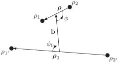
Figure 2: Relevant variables in the collision of two dipoles viewed in the transverse plane.

Let us start from the well-known BFKL amplitude Lipatov86

$${\cal A}(s,q^{2})=is\int\frac{d\omega}{2i\pi}e^{\omega Y}f_{\omega}(q^{2}),$$

where $s=e^{Y}$ is the centre-of-mass energy squared and $q$ is the momentum transfer. One writes Lipatov86

$$f_{\omega}(q^{2})\delta^{(2)}(\mathbf{q}-\mathbf{q}^{\prime}) = \int\prod_{i}\frac{d^{2}\rho_{i}}{(2\pi)^{2}}\,e^{i\frac{1}{2}(\boldsymbol{\rho}_{1}+\boldsymbol{\rho}_{2}).\mathbf{q}}\,\Phi_{P}(\boldsymbol{\rho},\mathbf{q})f_{\omega}(\boldsymbol{\rho}_{1},\boldsymbol{\rho}_{2},\boldsymbol{\rho}_{1^{\prime}},\boldsymbol{\rho}_{2^{\prime}})e^{-i\frac{1}{2}(\boldsymbol{\rho}_{1^{\prime}}+\boldsymbol{\rho}_{2^{\prime}}).\mathbf{q}^{\prime}}\,\Phi_{T}(\boldsymbol{\rho}_{0},\mathbf{q}^{\prime}),$$

$$f_{\omega}(\boldsymbol{\rho}_{1},\boldsymbol{\rho}_{2},\boldsymbol{\rho}_{1^{\prime}},\boldsymbol{\rho}_{2^{\prime}}) = \int_{-\infty}^{\infty}\frac{\nu^{2}\,d\nu}{2\pi(\nu^{2}+1/4)^{2}}\frac{1}{\omega-\bar{\alpha}\chi(\nu)}\int d^{2}r\,E^{\nu}(\boldsymbol{\rho}_{1}\!-\!\mathbf{r},\boldsymbol{\rho}_{2}\!-\!\mathbf{r})\bar{E}^{\nu}(\boldsymbol{\rho}_{1^{\prime}}\!-\!\mathbf{r},\boldsymbol{\rho}_{2^{\prime}}\!-\!\mathbf{r})$$ (9)

where

$$E^{\nu}(\boldsymbol{\rho}_{1},\boldsymbol{\rho}_{2})=\left(\frac{|\boldsymbol{\rho}_{1}-\boldsymbol{\rho}_{2}|}{|\boldsymbol{\rho}_{1}||\boldsymbol{\rho}_{2}|}\right)^{1+2i\nu}$$

are the conformal eigenfunctions of the BFKL kernel with vanishing conformal spin quantum number ($n=0$ in the usual terminology Lipatov86 ). It corresponds to the dominant contribution at high energy. $\Phi_{P}$ (resp. $\Phi_{T}$) are the impact factors describing the coupling of the BFKL pomeron to the projectile (resp. target), depending on the momentum transfer $\mathbf{q}$ and on the dipole sizes $\boldsymbol{\rho}\!=\!\boldsymbol{\rho}_{1}\!-\!\boldsymbol{\rho}_{2}$ and $\boldsymbol{\rho}_{0}\!=\!\boldsymbol{\rho}_{1^{\prime}}\!-\!\boldsymbol{\rho}_{2^{\prime}}$.

The Dirac distribution which appears in the definition of $f_{\omega}(q^{2})$ comes from the fact that, the global system being invariant under translation, the expression in the right-hand-side does not depend on $\boldsymbol{\rho}_{1}\!+\!\boldsymbol{\rho}_{2}\!+\!\boldsymbol{\rho}_{1^{\prime}}\!+\!\boldsymbol{\rho}_{2^{\prime}}$. To be more precise, the relevant variables of this problem are the sizes of the two dipoles, $\boldsymbol{\rho}$ and $\boldsymbol{\rho}_{0}$, and the impact parameter $\mathbf{b}\!=\!\frac{1}{2}(\boldsymbol{\rho}_{1}\!+\!\boldsymbol{\rho}_{2}\!-\!\boldsymbol{\rho}_{1^{\prime}}\!-\!\boldsymbol{\rho}_{2^{\prime}})$, as shown on Fig.2. Combining these expressions and using $\gamma=\frac{1}{2}+i\nu$ instead of $\nu$, we obtain the following expression for the amplitude

$${\cal A}(s,q^{2})=\frac{is}{(2\pi)^{6}}\int d^{2}b\,d^{2}\rho\,d^{2}\rho_{0}\,e^{i\mathbf{q}.\mathbf{b}}\Phi_{P}(\boldsymbol{\rho},\mathbf{q})\Phi_{T}(\boldsymbol{\rho}_{0},\mathbf{q})\int_{\frac{1}{2}-i\infty}^{\frac{1}{2}+i\infty}\frac{d\gamma}{2i\pi}\,e^{\bar{\alpha}\chi(\gamma)Y}f^{\gamma}(\boldsymbol{\rho},\boldsymbol{\rho}_{0},\mathbf{b}),$$ (10)

where we have introduced the function $f^{\gamma}$ as the result of the integration over $\mathbf{r}$ in (9)

$$f^{\gamma}(\boldsymbol{\rho},\boldsymbol{\rho}_{0},\mathbf{b})=\frac{-\left(\gamma-\frac{1}{2}\right)^{2}}{\gamma^{2}(1-\gamma)^{2}}\int d^{2}r\,E^{\gamma}(\boldsymbol{\rho}_{1}\!-\!\mathbf{r},\boldsymbol{\rho}_{2}\!-\!\mathbf{r})\bar{E}^{\gamma}(\boldsymbol{\rho}_{1^{\prime}}\!-\!\mathbf{r},\boldsymbol{\rho}_{2^{\prime}}\!-\!\mathbf{r}).$$

Using the complex representation for the two-dimensional vectors (in this section, we keep bold characters for vectors and ordinary ones for complex numbers), it has been shown LipatovReview ; NP that the result of this integration is

$$f^{\gamma}(\rho,\rho_{0},b)=\frac{c_{\gamma}}{\gamma^{2}(1-\gamma^{2})}\left|z\right|^{2\gamma}{}_{2}{\rm F}_{1}(\gamma,\gamma;2\gamma;z){}_{2}{\rm F}_{1}(\gamma,\gamma;2\gamma;\bar{z})+(\gamma\leftrightarrow 1-\gamma),$$

where ${}_{2}{\rm F}_{1}$ is the Gauss hypergeometric function math , the pre-factor

$$c_{\gamma}=\pi\,2^{1-4\gamma}\frac{\Gamma(\gamma)\,\Gamma\left(\frac{3}{2}-\gamma\right)}{\Gamma(1-\gamma)\Gamma\left(\gamma-\frac{1}{2}\right)}\,,$$ (11)

and

$$z=\frac{\rho_{12}\rho_{1^{\prime}2^{\prime}}}{\rho_{11^{\prime}}\rho_{22^{\prime}}}\equiv\frac{4\rho\rho_{0}}{4b^{2}-(\rho-\rho_{0})^{2}}$$ (12)

is the anharmonic ratio. This is a remarkable property due to conformal invariance that the BFKL pomeron exchange in coordinate space depends on $\rho$, $\rho_{0}$ and $b$ only through the anharmonic ratio $z$.

Since we are interested in the situation where one small dipole of size $\rho$ scatters on a larger one of size $\rho_{0}$, i.e. $\left|\rho\right|\ll\left|\rho_{0}\right|$, we can expand $f^{\gamma}(\rho,\rho_{0},b)$ in series of $\rho/\rho_{0}$. In that limit, the hypergeometric function goes to 1 and we obtain

$$f^{\gamma}(\rho,\rho_{0},b)\approx\frac{c_{\gamma}}{\gamma^{2}(1-\gamma)^{2}}\left|\frac{4\rho\rho_{0}}{4b^{2}-\rho_{0}^{2}}\right|^{2\gamma}+(\gamma\leftrightarrow 1-\gamma).$$ (13)

Before going any further, one has to point out that the corrections to this expression are of order $(\rho/\rho_{0})^{2}$ but reduce to $(\rho/\rho_{0})^{4}$ if we integrate over the phase $\phi$ of $\rho$ (see Fig.2 for the kinematics).

The expression (13) still depends on the angle $\phi_{0}$ between $\rho_{0}$ and $b$. Since this is not relevant for phenomenological studies, it is interesting to integrate this result over the phases $\phi$ and $\phi_{0}$ of $\rho$ and $\rho_{0}$ (one may assume that $b$ is real). One obtains

$$\left\langle f^{\gamma}(\rho,\rho_{0},b)\right\rangle_{\phi,\phi_{0}}=\frac{c_{\gamma}}{\gamma^{2}(1-\gamma)^{2}}\left(\frac{4\left|\rho\right|\left|\rho_{0}\right|}{\left|\left|\rho_{0}\right|^{2}-4\left|b\right|^{2}\right|}\right)^{2\gamma}P_{\gamma-1}\left(\frac{\left|\rho_{0}\right|^{4}+16\left|b\right|^{4}}{\left|\left|\rho_{0}\right|^{4}-16\left|b\right|^{4}\right|}\right)+(\gamma\leftrightarrow 1-\gamma),$$ (14)

where $P_{\gamma-1}(x)$ is the Legendre function of the first kind math .

Finally, if we additionally take $b$ going to zero in this result, we obtain

$$\left\langle f^{\gamma}(\rho,\rho_{0},0)\right\rangle_{\phi,\phi_{0}}=\frac{1}{\gamma^{2}(1-\gamma)^{2}}\left(c_{\gamma}\left|\frac{4\rho}{\rho_{0}}\right|^{2\gamma}+c_{1-\gamma}\left|\frac{4\rho}{\rho_{0}}\right|^{2-2\gamma}\right)$$ (15)

which exhibits the same power behaviour as in the forward case.

III.2 Mixed space

It is useful to introduce a mixed space representation Lipatov86 in terms of $\rho$, $\rho_{0}$ and $q$. One obtains from (10)

$${\cal{A}}(s,q^{2})=\frac{is}{(2\pi)^{4}}\int d^{2}\rho\,d^{2}\rho_{0}\,\Phi_{P}(\boldsymbol{\rho},\mathbf{q})\Phi_{T}(\boldsymbol{\rho}_{0},\mathbf{q})\int_{-\infty}^{\infty}\frac{d\nu}{2\pi}\,f_{q}^{\nu}(\boldsymbol{\rho},\boldsymbol{\rho}_{0})\,e^{\bar{\alpha}\chi(\nu)Y}$$ (16)

where

$$f_{q}^{\nu}(\boldsymbol{\rho},\boldsymbol{\rho}_{0})=\int\frac{d^{2}b}{(2\pi)^{2}}\,e^{i\mathbf{q}.\mathbf{b}}\,f^{\nu}(\boldsymbol{\rho},\boldsymbol{\rho}_{0},\mathbf{b})=\frac{\left|\boldsymbol{\rho}\right|\left|\boldsymbol{\rho}_{0}\right|}{16(\nu^{2}+1/4)^{2}}\bar{E}_{q}^{\nu}(\boldsymbol{\rho}_{0})E_{q}^{\nu}(\boldsymbol{\rho})$$ (17)

acquires a factorised form with

$$E_{q}^{\nu}(\boldsymbol{\rho})=\frac{4c_{\gamma}}{\pi^{2}|\boldsymbol{\rho}|}\int d^{2}z\ e^{i\mathbf{q}.\mathbf{z}}E^{\nu}\left(\mathbf{z}+\frac{\boldsymbol{\rho}}{2},\mathbf{z}-\frac{\boldsymbol{\rho}}{2}\right).$$

Using again the complex representation for the two-dimensional vectors, one finds (see NP )

$$E_{q}^{\nu}(\rho)=\left|q\right|^{2i\nu}2^{-6i\nu}\Gamma^{2}(1-i\nu)\left[J_{-i\nu}\left(\frac{\bar{q}\rho}{4}\right)J_{-i\nu}\left(\frac{q\bar{\rho}}{4}\right)-J_{i\nu}\left(\frac{\bar{q}\rho}{4}\right)J_{i\nu}\left(\frac{q\bar{\rho}}{4}\right)\right]\quad\text{and}\qquad\bar{E}_{q}^{\nu}(\rho_{0})=E_{q}^{-\nu}(\rho_{0})\,,$$

where $J_{\alpha}\left(z\right)$ is the Bessel function of the first kind. Using $\gamma=\frac{1}{2}+i\nu$ instead of $\nu$, the $(\nu\leftrightarrow-\nu)$ symmetry turns into a $(\gamma\leftrightarrow 1-\gamma)$ symmetry and we finally get

$$f_{q}^{\gamma}(\rho,\rho_{0})=\frac{\left|\rho\rho_{0}\right|}{16\gamma^{2}(1-\gamma)^{2}}\Gamma^{2}\left(\frac{3}{2}-\gamma\right)\Gamma^{2}\left(\frac{1}{2}+\gamma\right) \left[J_{\frac{1}{2}-\gamma}\left(\frac{\bar{q}\rho}{4}\right)J_{\frac{1}{2}-\gamma}\left(\frac{q\bar{\rho}}{4}\right)-J_{\gamma-\frac{1}{2}}\left(\frac{\bar{q}\rho}{4}\right)J_{\gamma-\frac{1}{2}}\left(\frac{q\bar{\rho}}{4}\right)\right]$$ (18)

$$\times \left[J_{\gamma-\frac{1}{2}}\left(\frac{\bar{q}\rho_{0}}{4}\right)J_{\gamma-\frac{1}{2}}\left(\frac{q\bar{\rho}_{0}}{4}\right)-J_{\frac{1}{2}-\gamma}\left(\frac{\bar{q}\rho_{0}}{4}\right)J_{\frac{1}{2}-\gamma}\left(\frac{q\bar{\rho}_{0}}{4}\right)\right]\,.$$

Let us notice that this expression has the crucial feature that it is factorised in $\rho$ and $\rho_{0}$ by contrast with the $b$ representation. This property, inherent to the fact that we use the momentum transfer $q$ instead of the impact parameter $b$, will be of prime importance for obtaining the solutions of the BK equation.

As explained before, we are interested in the situation where one dipole is much larger than the other one ($\rho_{0}\gg\rho$). In order to expand the Bessel functions in series of their respective arguments, we shall consider three situations: $\rho_{0}\gg\rho\gg 1/q$, $\rho_{0}\gg 1/q\gg\rho$ and $1/q\gg\rho_{0}\gg\rho$. The results then follow from the asymptotic expansion of the Bessel functions

$$J_{\mu}\left(z\right)J_{\mu}\left(\bar{z}\right)-J_{-\mu}\left(z\right)J_{-\mu}\left(\bar{z}\right) \stackrel{{\scriptstyle\left|z\right|\ll 1}}{{\longrightarrow}} \frac{1}{\Gamma^{2}(1+\mu)}\left|\frac{z}{2}\right|^{2\mu}-\frac{1}{\Gamma^{2}(1-\mu)}\left|\frac{z}{2}\right|^{-2\mu},$$ (19)

$$\stackrel{{\scriptstyle\left|z\right|\gg 1}}{{\longrightarrow}} \frac{-2}{\pi\left|z\right|}\sin(\mu\pi)\cos\left[2\Re e(z)\right].$$ (20)

Using these expressions we obtain the following results for the three relevant cases.

• Case 1: $1/q\gg\rho_{0}\gg\rho$.
  Using (18) and (19), we find

  $$f_{q}^{\gamma}(\rho,\rho_{0}) = \frac{\left|\rho\rho_{0}\right|}{16\gamma^{2}(1-\gamma)^{2}}\Gamma^{2}\left(\frac{3}{2}-\gamma\right)\Gamma^{2}\left(\frac{1}{2}+\gamma\right)$$

  $$\times \left[\frac{1}{\Gamma^{2}\left(\frac{3}{2}-\gamma\right)}\left|\frac{\rho q}{8}\right|^{1-2\gamma}-\frac{1}{\Gamma^{2}\left(\frac{1}{2}+\gamma\right)}\left|\frac{\rho q}{8}\right|^{2\gamma-1}\right]\left[\frac{1}{\Gamma^{2}\left(\frac{1}{2}+\gamma\right)}\left|\frac{\rho_{0}q}{8}\right|^{2\gamma-1}-\frac{1}{\Gamma^{2}\left(\frac{3}{2}-\gamma\right)}\left|\frac{\rho_{0}q}{8}\right|^{1-2\gamma}\right].$$

  In particular, if we take $q\to 0$ in this expression, we recover

  $$f_{q}^{\gamma}(\rho,\rho_{0})\stackrel{{\scriptstyle q\to 0}}{{\longrightarrow}}\frac{\left|\rho\rho_{0}\right|}{16\gamma^{2}(1-\gamma)^{2}}\left(\left|\frac{\rho}{\rho_{0}}\right|^{1-2\gamma}+\left|\frac{\rho}{\rho_{0}}\right|^{2\gamma-1}\right).$$ (21)

• Case 2: $\rho_{0}\gg 1/q\gg\rho$.
  Due to the asymptotic expansion (20), the $\rho_{0}$ part will not depend on $\gamma$ anymore and we obtain

  $$f_{q}^{\gamma}(\rho,\rho_{0})=\frac{-1}{2\pi}\frac{\cos(\gamma\pi)}{\gamma^{2}(1-\gamma)^{2}}\cos\left[\frac{\Re e(\rho_{0}\bar{q})}{2}\right]\frac{1}{\left|q\right|^{2}}\left[\Gamma^{2}\left(\frac{3}{2}-\gamma\right)\left|\frac{\rho q}{8}\right|^{2\gamma}-\Gamma^{2}\left(\frac{1}{2}+\gamma\right)\left|\frac{\rho q}{8}\right|^{2-2\gamma}\right].$$ (22)

  Note that this amplitude still depends on the angle $\psi_{0}$ between $q$ and $\rho_{0}$. If we integrate out this angle together with the dependence on the angle $\psi$ between $q$ and $\rho$, we have

  $$\left\langle f_{q}^{\gamma}(\rho,\rho_{0})\right\rangle_{\psi,\psi_{0}}=\frac{-\cos(\gamma\pi)}{\gamma^{2}(1-\gamma)^{2}}\cos\left(\frac{\left|\rho_{0}q\right|}{2}-\frac{\pi}{4}\right)\sqrt{\frac{1}{\pi^{3}\left|\rho_{0}q^{3}\right|}}\left[\Gamma^{2}\left(\frac{3}{2}-\gamma\right)\left|\frac{\rho q}{8}\right|^{2\gamma}-\Gamma^{2}\left(\frac{1}{2}+\gamma\right)\left|\frac{\rho q}{8}\right|^{2-2\gamma}\right].$$ (23)

• Case 3: $\rho_{0}\gg\rho\gg 1/q$.
  In this case, both the $\rho$- and $\rho_{0}$-dependent parts of (18) involve expansion (20) which gives

  $$f_{q}^{\gamma}(\rho,\rho_{0})=\frac{-4}{\pi^{2}}\frac{\cos^{2}(\gamma\pi)}{\gamma^{2}(1-\gamma)^{2}}\Gamma^{2}\left(\frac{1}{2}+\gamma\right)\Gamma^{2}\left(\frac{3}{2}-\gamma\right)\frac{1}{\left|q\right|^{2}}\cos\left[\frac{\Re e(\rho\bar{q})}{2}\right]\cos\left[\frac{\Re e(\rho_{0}\bar{q})}{2}\right]$$ (24)

  and, averaging over the angles $\psi$ and $\psi_{0}$,

  $$\left\langle f_{q}^{\gamma}(\rho,\rho_{0})\right\rangle_{\psi,\psi_{0}}=\frac{-16}{\pi^{4}}\frac{\cos^{2}(\gamma\pi)}{\gamma^{2}(1-\gamma)^{2}}\Gamma^{2}\left(\frac{1}{2}+\gamma\right)\Gamma^{2}\left(\frac{3}{2}-\gamma\right)\frac{1}{\left|\rho\rho_{0}q^{4}\right|}\cos\left(\frac{\left|\rho q\right|}{2}-\frac{\pi}{4}\right)\cos\left(\frac{\left|\rho_{0}q\right|}{2}-\frac{\pi}{4}\right).$$ (25)

III.3 Momentum space

The situation in momentum space is very similar to the one in mixed space. If we still neglect the contribution of higher conformal spins, we find

$${\cal A}(s,q^{2})=is\int d^{2}k\,d^{2}k_{0}\,\Phi_{P}(\mathbf{k},\mathbf{q})\Phi_{T}(\mathbf{k}_{0},\mathbf{q})\int_{-\infty}^{\infty}\frac{d\nu}{2\pi}\,e^{\bar{\alpha}\chi(\nu)Y}f^{\nu}(\mathbf{k},\mathbf{k}_{0},\mathbf{q}),$$ (26)

where $\Phi_{P}$ and $\Phi_{T}$ are the impact factors in momentum space

$$\Phi_{P}(\mathbf{k},\mathbf{q})=\int\frac{d^{2}\rho}{(2\pi)^{2}}\,e^{-i(\mathbf{k}-\mathbf{q}/2).\boldsymbol{\rho}}\,\Phi_{P}(\boldsymbol{\rho},\mathbf{q}),$$

and $f^{\nu}(\mathbf{k},\mathbf{k}_{0},\mathbf{q})$ is the Fourier transform of $f_{q}^{\nu}(\boldsymbol{\rho},\boldsymbol{\rho}_{0})$:

$$f^{\nu}(\mathbf{k},\mathbf{k}_{0},\mathbf{q})=\frac{1}{(2\pi)^{4}}\frac{1}{(\nu^{2}+1/4)^{2}}\int d^{2}\rho\,e^{i(\mathbf{k}-\mathbf{q}/2).\boldsymbol{\rho}}\,\frac{\left|\boldsymbol{\rho}\right|}{4}E_{q}^{\nu}(\boldsymbol{\rho})\int d^{2}\rho_{0}\,e^{i(\mathbf{k}_{0}-\mathbf{q}/2).\boldsymbol{\rho}_{0}}\,\frac{\left|\boldsymbol{\rho}_{0}\right|}{4}\bar{E}_{q}^{\nu}(\boldsymbol{\rho}_{0}).$$ (27)

The detailed calculation of this integral is presented in Appendix A and the relation with conformal invariance is developed in Appendix B. The final expression, using again the complex representation (see footnote 4) and replacing $\nu$ by $\gamma=\frac{1}{2}+i\nu$, is

$$f^{\gamma}(k,k_{0},q) = \frac{-1}{(2\pi)^{4}}\frac{\sin^{2}(\gamma\pi)}{16\gamma^{2}(1-\gamma)^{2}}\Gamma^{2}\left(\frac{1}{2}+\gamma\right)\Gamma^{2}\left(\frac{3}{2}-\gamma\right)\left(\frac{4}{\left|kk_{0}\right|}\right)^{3}$$ (28)

$$\times \left[\frac{\Gamma^{2}(1+\gamma)}{\Gamma^{2}\left(\frac{1}{2}+\gamma\right)}\left|\frac{q}{4k}\right|^{2\gamma-1}{}_{2}{\rm F}_{1}\left(\gamma,1+\gamma;2\gamma;\frac{q}{k}\right){}_{2}{\rm F}_{1}\left(\gamma,1+\gamma;2\gamma;\frac{\bar{q}}{\bar{k}}\right)-(\gamma\leftrightarrow 1-\gamma)\right]$$

$$\times \left[\frac{\Gamma^{2}(1+\gamma)}{\Gamma^{2}\left(\frac{1}{2}+\gamma\right)}\left|\frac{q}{4k_{0}}\right|^{2\gamma-1}{}_{2}{\rm F}_{1}\left(\gamma,1+\gamma;2\gamma;\frac{q}{k_{0}}\right){}_{2}{\rm F}_{1}\left(\gamma,1+\gamma;2\gamma;\frac{\bar{q}}{\bar{k}_{0}}\right)-(\gamma\leftrightarrow 1-\gamma)\right].$$

As in the mixed space representation, this expression has the remarkable property of being factorised in $k$ and $k_{0}$. This appears from the fact that we use the momentum transfer $q$ and is lost if we go back to impact-parameter $b$.

We can now consider these expressions in the case where one dipole is much harder than the other, corresponding to $k\gg k_{0}$. Thanks to the fact that $f^{\gamma}$ is factorised in $q/k$ and $q/k_{0}$, we again need to consider three situations: $k\gg k_{0}\gg q$, $k\gg q\gg k_{0}$ and $q\gg k\gg k_{0}$. When $q$ is small compared to $k$, it is sufficient to consider

$${}_{2}{\rm F}_{1}\left(\gamma,1+\gamma;2\gamma;\frac{q}{k}\right)\stackrel{{\scriptstyle\left|k\right|\gg\left|q\right|}}{{\approx}}1\,.$$

The behaviour at large $q$ is more complicated. We show in Appendix C that, averaging over the angle $\theta$ between $k$ and $q$, we have

$$\left\langle\frac{\Gamma^{2}(1+\gamma)}{\Gamma^{2}\left(\frac{1}{2}+\gamma\right)}\left|\frac{q}{4k}\right|^{2\gamma-1}{}_{2}{\rm F}_{1}\left(\gamma,1+\gamma;2\gamma;\frac{q}{k}\right){}_{2}{\rm F}_{1}\left(\gamma,1+\gamma;2\gamma;\frac{\bar{q}}{\bar{k}}\right)-(\gamma\leftrightarrow 1-\gamma)\right\rangle_{\!\theta}$$

$$\stackrel{{\scriptstyle\left|k\right|\ll\left|q\right|}}{{\longrightarrow}}4\gamma^{2}(1-\gamma)^{2}\frac{\cos(\gamma\pi)}{\sin(\gamma\pi)}\left|\frac{q}{k}\right|^{-3}\,\log\left|\frac{q}{k}\right|.$$ (29)

Before considering the three cases in more details, one may note that the $q^{-3}$ behaviour could have been anticipated from the fact that, in that limit, the Fourier transform of $E_{q}^{\nu}(\rho)$ does not depend on $k$. Note however the logarithmic term arising from the hypergeometric function.

Let us now consider the results for the three different cases.

• Case 1: $k\gg k_{0}\gg q$.
  In this case, both parts of the expression show a power behaviour,

  $$f^{\gamma}(k,k_{0},q) = \frac{-1}{\pi^{4}}\frac{\sin^{2}(\gamma\pi)}{4\gamma^{2}(1-\gamma)^{2}}\Gamma^{2}\left(\frac{3}{2}-\gamma\right)\Gamma^{2}\left(\frac{1}{2}+\gamma\right)\frac{1}{\left|kk_{0}\right|^{3}}$$

  $$\times \left[\frac{\Gamma^{2}\left(1+\gamma\right)}{\Gamma^{2}\left(\frac{1}{2}+\gamma\right)}\left|\frac{q}{4k}\right|^{2\gamma-1}-\frac{\Gamma^{2}\left(2-\gamma\right)}{\Gamma^{2}\left(\frac{3}{2}-\gamma\right)}\left|\frac{q}{4k}\right|^{1-2\gamma}\right]\left[\frac{\Gamma^{2}\left(1+\gamma\right)}{\Gamma^{2}\left(\frac{1}{2}+\gamma\right)}\left|\frac{q}{4k_{0}}\right|^{2\gamma-1}-\frac{\Gamma^{2}\left(2-\gamma\right)}{\Gamma^{2}\left(\frac{3}{2}-\gamma\right)}\left|\frac{q}{4k_{0}}\right|^{1-2\gamma}\right]$$

  $$= \frac{1}{(2\pi)^{2}}\frac{1}{\left|kk_{0}\right|^{3}}\left[\left|\frac{k}{k_{0}}\right|^{1-2\gamma}-\frac{\sin^{2}(\gamma\pi)}{16\pi^{2}\gamma^{2}(1-\gamma)^{2}}\frac{\Gamma^{4}(1+\gamma)\Gamma^{2}\left(\frac{3}{2}-\gamma\right)}{\Gamma^{2}\left(\frac{1}{2}+\gamma\right)}\left|\frac{q^{2}}{16kk_{0}}\right|^{2\gamma-1}+(\gamma\to 1-\gamma)\right].$$

  In the distributed product, we clearly see that, taking the limit $q\to 0$, we recover an expression depending only on the ratio between the momenta of the two dipoles

  $$f^{\gamma}(k,k_{0},q)\stackrel{{\scriptstyle q\to 0}}{{\longrightarrow}}\frac{1}{(2\pi)^{2}}\frac{1}{\left|kk_{0}\right|^{3}}\left(\left|\frac{k}{k_{0}}\right|^{1-2\gamma}+\left|\frac{k}{k_{0}}\right|^{2\gamma-1}\right).$$ (31)

• Case 2: $k\gg q\gg k_{0}$.
  At intermediate values of $q$, the dependence on $k_{0}$ goes away and we recover an analytic power behaviour in $\gamma$ which, as we shall see in the next section, will lead to traveling waves and geometric scaling

  $$f^{\gamma}(k,k_{0},q) = \frac{-1}{2\pi^{4}}\sin(2\gamma\pi)\Gamma^{2}\left(\frac{3}{2}-\gamma\right)\Gamma^{2}\left(\frac{1}{2}+\gamma\right)$$ (32)

  $$\log\left|\frac{q}{k_{0}}\right|\frac{1}{\left|kq\right|^{3}}\left[\frac{\Gamma^{2}\left(1+\gamma\right)}{\Gamma^{2}\left(\frac{1}{2}+\gamma\right)}\left|\frac{q}{4k}\right|^{2\gamma-1}-\frac{\Gamma^{2}\left(2-\gamma\right)}{\Gamma^{2}\left(\frac{3}{2}-\gamma\right)}\left|\frac{q}{4k}\right|^{1-2\gamma}\right].$$

• Case 3: $q\gg k\gg k_{0}$.
  This limit gives

  $$f^{\gamma}(k,k_{0},q)=\frac{-4}{\pi^{4}}\cos^{2}(\gamma\pi)\Gamma^{2}\left(\frac{3}{2}-\gamma\right)\Gamma^{2}\left(\frac{1}{2}+\gamma\right)\gamma^{2}(1-\gamma)^{2}\frac{1}{\left|q\right|^{6}}\log\left|\frac{q}{k_{0}}\right|\log\left|\frac{q}{k}\right|.$$ (33)

IV Traveling waves at nonzero transfer

In this section, we investigate the consequences of our formulæ for linear BFKL dynamics on asymptotic solutions when the non-linear effects of the BK equation are switched on. The key point is that linear BFKL dynamics can provide solutions for the linear part of the BK equation. Indeed, when factorisation between the target and the projectile is fulfilled, the impact factor of the target can be integrated out keeping a linear evolution governed by the same kernel. It is thus a solution of the linear part of the BK equation which should depend only on the kinematic variables of the projectile.

In the next step, the asymptotic solutions of the BK equation can be deduced from the knowledge of its linear part, using quite general arguments which were recalled in Sections I and II. For each of the kinematical configurations introduced in the previous section, we check whether the conditions for the existence of traveling waves are fulfilled and, in these cases, derive their expression.

Let us first concentrate on the full momentum representation (26). We define the function

$$f(\mathbf{k},\mathbf{q})=\int d^{2}k_{0}\,\Phi_{T}(\mathbf{k}_{0},\mathbf{q})\int\frac{d\gamma}{2i\pi}\,e^{\bar{\alpha}\chi(\gamma)Y}f^{\gamma}(\mathbf{k},\mathbf{k}_{0},\mathbf{q}),$$ (34)

depending only on $\mathbf{k}$ and $\mathbf{q}$. It is remarkable that in this representation, the exact factorisation property of $f^{\gamma}(\mathbf{k},\mathbf{k}_{0},\mathbf{q})$ (see (27)) gives rise to the simple expression

$$f(\mathbf{k},\mathbf{q})=\int\frac{d\gamma}{2i\pi}\,e^{\bar{\alpha}\chi(\gamma)Y}\phi^{\gamma}(\mathbf{q})\,f^{\gamma}(\mathbf{k},\mathbf{q}),$$ (35)

where

$$\phi^{\gamma}(\mathbf{q})=\int d^{2}k_{0}\,\frac{d^{2}\rho_{0}}{(2\pi)^{2}}\,e^{i(\mathbf{k}_{0}-\mathbf{q}/2).\boldsymbol{\rho}_{0}}\,\frac{\left|\boldsymbol{\rho}_{0}\right|}{4}\bar{E}_{q}^{\gamma}(\boldsymbol{\rho}_{0})\Phi_{T}(\mathbf{k}_{0},\mathbf{q})$$

factorises out the target dependence, defining the initial condition, and

$$f^{\gamma}(\mathbf{k},\mathbf{q})=\int\frac{d^{2}\rho}{(2\pi)^{2}}\,e^{i(\mathbf{k}-\mathbf{q}/2).\boldsymbol{\rho}}\,\frac{\left|\boldsymbol{\rho}\right|}{4}E_{q}^{\gamma}(\boldsymbol{\rho})$$

$$=\frac{2^{4-6\gamma}\,\Gamma^{2}\!\left(\frac{3}{2}-\gamma\right)}{(2\pi)^{2}}\sin(\gamma\pi)\frac{\left|q\right|^{2\gamma-1}}{\left|k\right|^{3}}\left[\frac{\Gamma^{2}\!\left(1+\gamma\right)}{\Gamma^{2}\!\left(\frac{1}{2}+\gamma\right)}\left|\frac{q}{4k}\right|^{2\gamma-1}{}_{2}{\rm F}_{1}\!\left(\gamma+1,\gamma;2\gamma;\frac{q}{k}\right){}_{2}{\rm F}_{1}\!\left(\gamma+1,\gamma;2\gamma;\frac{\bar{q}}{\bar{k}}\right)-(\gamma\to 1-\gamma)\right]$$

is calculated in Appendix B and enters in formula (28). It is obvious from the structure of (34), a linear superposition of eigenfunctions of the BFKL kernel, that it provides a natural basis for the solutions of the linear part of the BK equation in momentum space.

Therefore, we look for the kinematical domains where $f^{\gamma}(\mathbf{k},\mathbf{q})$ takes the appropriate exponential behaviour, corresponding to the wave superposition property (4) discussed in section II. It will lead to traveling-wave solutions for the full BK equation.

We observe that, both in the cases 1 and 2 (formulæ (31) and (32)), i.e. in the limit $k\!\gg\!q$, the solution of the linear part of the BK equation can be recast, using the symmetry $\gamma\leftrightarrow 1-\gamma$, under the form

$$f(\mathbf{k},\mathbf{q})=\frac{1}{k^{2}}\int\frac{d\gamma}{2i\pi}\,\phi^{\gamma}(\mathbf{q})\,e^{\bar{\alpha}\chi(\gamma)Y-\gamma L},$$

where

$$L=\log\left(\frac{k^{2}}{q^{2}}\right)$$

expresses the leading power-like behaviour at large $k/q$ and all remaining factors in $\gamma$ and $\mathbf{q}$ has been reabsorbed in $\phi^{\gamma}(\mathbf{q})$. This clearly emphasises the fact that the region of interest is $k\!\gg\!q$, independently of $k_{0}$. By contrast, in the case 3 treating the large-$q$ expression, we see that equation (33), though being factorised, does not fulfil the same property. We thus do not expect traveling-wave solutions in this limit.

Let us now include the effect of the nonlinear term in the BK equation. Due to colour transparency ($f(\mathbf{k},\mathbf{q})\sim k^{-2}$ for $k\gg q$), one can apply the general arguments exposed in Section II. Therefore, the solution of the BK equation reaches asymptotically the traveling-wave structure and exhibits geometric scaling. The saturation scale

$$Q_{s}^{2}(Y) = q^{2}\Omega_{s}^{2}(Y)$$

$$\sim q^{2}\exp\left[\bar{\alpha}\frac{\chi(\gamma_{c})}{\gamma_{c}}Y-\frac{3}{2\gamma_{c}}\log(Y)\right]$$

has the same rapidity dependence as in the forward case but is proportional to the momentum transfer. The critical exponent $\gamma_{c}$ is still given by equation (6). The asymptotic form of the amplitude, i.e. the wavefront, can be written at small $q/k$

$$f(\mathbf{k},\mathbf{q})\stackrel{{\scriptstyle Y\to\infty}}{{\sim}}\frac{1}{k^{2}}\,\phi^{\gamma_{c}}(\mathbf{q})\,\log\left(\frac{k^{2}}{q^{2}\Omega_{s}^{2}(Y)}\right)\,\left|\frac{k^{2}}{q^{2}\Omega_{s}^{2}(Y)}\right|^{-\gamma_{c}}\,\exp\left[-\frac{1}{2\bar{\alpha}\chi^{\prime\prime}(\gamma_{c})Y}\log^{2}\left(\frac{k^{2}}{q^{2}\Omega_{s}^{2}(Y)}\right)\right].$$ (38)

It is interesting to see how we recover the forward limit $\mathbf{q}\to 0$ recalled in Section II. This can be done remarking that formula (• ‣ III.3), obtained for BFKL dynamics in the case 1 ($k\gg k_{0}\gg q$), introduces and additional factor $(q/k_{0})^{-2\gamma}$. By recombination of the $q/k$ and $q/k_{0}$ factors, a different factorisation appear where $k_{0}$ substitute to $q$ as the reference scale, as clearly seen in (31). Inserting (31) in (34), by straightforward algebra, it is easy to see that the result can be cast under the form

$$f(\mathbf{k},\mathbf{q}\to 0)=\frac{1}{k^{2}}\int\frac{d\gamma}{2i\pi}\,\phi^{\gamma}(Q_{T})\,e^{\bar{\alpha}\chi(\gamma)Y-\gamma L_{0}},$$

where

$$L_{0}=\log\left(\frac{k^{2}}{Q_{T}^{2}}\right),$$

and $Q_{T}$ is a scale typical for the target, defining the initial condition for the traveling-wave solution. This corresponds to the solutions of equation (2).

This discussion can be translated to the amplitude in the mixed space representation of section III.1 defining similarly

$$f(\boldsymbol{\rho},\mathbf{q})=\int\frac{d^{2}\rho_{0}}{(2\pi)^{2}}\,\Phi_{T}(\boldsymbol{\rho}_{0},\mathbf{q})\int\frac{d\gamma}{2i\pi}e^{\bar{\alpha}\chi(\gamma)Y}f_{q}^{\gamma}(\boldsymbol{\rho},\boldsymbol{\rho}_{0}),$$

where $f_{q}^{\gamma}(\boldsymbol{\rho},\boldsymbol{\rho}_{0})$, given by (17), is the solution of the BFKL equation in the mixed representation. As for the case of the momentum space, the factorisation of the target and projectile dependences in the BFKL amplitude is the important property, leading to traveling waves when we include the nonlinear effects in the limit $\rho\ll 1/q$.

The situation is not as simple in coordinate space. Indeed, it is hard to introduce an amplitude depending only on $\boldsymbol{\rho}$ and $\mathbf{b}$ from equation (10). This is closely related to the fact that $f^{\gamma}(\boldsymbol{\rho},\boldsymbol{\rho}_{0},\mathbf{b})$, depending only on the anharmonic ratio, cannot be factorised. In the limit where the BK equation is valid ($\rho_{0}\!\gg\!b,\rho$), its linear part gives solutions of the form (see (15)):

$$f(\boldsymbol{\rho},\mathbf{b})=\int\frac{d\gamma}{2i\pi}\frac{2c_{\gamma}}{\gamma^{2}(1-\gamma)^{2}}\,e^{\bar{\alpha}\chi(\gamma)Y}\,\left(\frac{4\rho}{\rho_{0}}\right)^{2\gamma},$$

where $\rho_{0}$ is the typical size of the target. As explained in Section II, this leads to traveling-wave solutions for the BK equation ${\cal N}(\rho,Y)\!=\!{\cal N}(\rho\ Q_{s}(Y))$, where all trace of the impact parameter has disappeared. Hence, it gives no information upon the $b$ dependence. We could instead consider equation (14) when the scaling variable $\rho\rho_{0}/|\rho_{0}^{2}-4b^{2}|$ is large, i.e. $\rho_{0}\sim 2b$. However, it is not clear whether the BK equation makes sense physically in that limit where the dipole hits the target in its peripheral region ($\rho_{0}\sim 2b$). As explained above, these difficulties arise from the fact that $\rho$ and $\rho_{0}$ are mixed non-trivially in the anharmonic ratio (12). Hence, an interpretation in term of the BK equation is problematic. By contrast, the situation in mixed and momentum spaces does not suffer this inconvenient, due to the nice factorisation property in $\rho$ and $\rho_{0}$, or in $k$ and $k_{0}$.

V Conclusions and perspectives

Let us first emphasise the main results of this paper. We show that traveling-wave solutions of the forward BK equation can be extended to the full equation including nonzero transfer $q$, provided that $k\gg q$, where $k$ represents the scale of the projectile. The saturation scale (IV) has the same energy dependence than in the forward case but is now proportional to $q$. When this scale is large w.r.t. the scale, e.g. $Q_{T}$, characterising the target, the saturation scale thus becomes independent of the details of the target. But, when the momentum transfer $q$ is small w.r.t. the target scale, $Q_{T}$ substitutes to $q$ in the saturation scale as expected from the forward case analysis. Our results show that non-forward BKFL evolution with momemtum transfer $q$ in a presence of saturation at the scale $\Omega_{s}(Y)$ is equivalent to forward BKFL evolution in the presence of saturation at the scale $q\Omega_{s}(Y)/Q_{T}.$ Note that the similarity of a momentum transfer with an absorptive boundary in BFKL evolution has been noticed in Ref.mueltri .

As a consequence of the existence of traveling-wave solutions, we derive the asymptotic form of the solution, i.e. the wavefront (38), at small $q/k$. It appears as an expression of the same form as in the forward case with two modifications: the saturation scale is now the proportional to $q$ and the pre-factor, related to the initial conditions, is now $q$-dependent.

From these considerations, we can predict that the BK equation implies the extension of geometric scaling at nonzero momentum transfer. Indeed, using formula (26) and noting that, at large $k$, the impact factor of the projectile is expected to scale with the ratio $k/Q$ where $Q$ is a typical hard scale of the projectile. We see that the amplitude satisfies the geometric scaling under the form

$${\cal{A}}(s,q^{2},Q^{2})\propto is\,\phi^{\gamma_{c}}(q)f\left(\frac{Q^{2}}{q^{2}\Omega^{2}_{s}(Y)}\right).$$ (39)

All these results apply also in the mixed-space representation depending on the projectile size $\rho$ and the momentum transfer $q$. However, we find that these properties seem not to be easily expressed in terms of the impact parameter.

Technically, the method used consists in three main steps. Firstly, we analyse the form of the BFKL solutions in full phase space and in different pertinent limits. Secondly, we use conformal-invariant properties of the BFKL dynamics to look for factorised solutions which then lead to solutions of the linear part of the BK equation. Thirdly, we infer the traveling-wave solutions, induced by nonlinear effects, in the kinematical regions and for initial conditions where the universality properties of the BK equation apply.

Some comments are in order. Our formula (38) suggests a solution to the puzzling problem of the compatibility of the BK equation with the confinement scale Kovner:2001bh ; Ferreiro:2002kv ; Bondarenko:2003ym ; Golec-Biernat:2003ym ; Gotsman:2004ra ; Ikeda:2004zp . The key point is to address the problem in momentum space where the non-perturbative dependence is factorised as clearly seen from the factor $\phi^{\gamma_{c}}(q)$ in equation (38), which may be characterised by a confinement scale. Fourier-transforming this result back to impact parameter space will break this factorisation property.

The properties of the BK solutions at nonzero momentum transfer suggest to analyse the high-energy behaviour of suitable experimental processes. The electroproduction of $\rho$-mesons at nonzero transfer has been already analysed in impact parameter space Munier:2001nr and our solutions of the BK equation incite to perform the analysis in momentum space.

Appendix A Calculation of $f^{\nu}(\mathbf{k},\mathbf{k}_{0},\mathbf{q})$

In this appendix, we compute the Fourier transform of

$$E_{q}^{\nu}(\rho)=2^{3\mu}\left|q\right|^{-2\mu}\Gamma^{2}(1+\mu)\left[J_{\mu}\left(\frac{\bar{q}\rho}{4}\right)J_{\mu}\left(\frac{q\bar{\rho}}{4}\right)-J_{-\mu}\left(\frac{\bar{q}\rho}{4}\right)J_{-\mu}\left(\frac{q\bar{\rho}}{4}\right)\right],$$ (40)

with $\mu=-i\nu$. It is of course sufficient to compute the following integral

$$I=\int d\rho\,d\phi\,\rho^{2+\alpha}e^{i\rho v\cos(\phi)}J_{\mu}\left(\frac{\left|q\right|\rho}{4}e^{i(\phi-\psi)}\right)J_{\mu}\left(\frac{\left|q\right|\rho}{4}e^{i(\psi-\phi)}\right),$$

where $v=\left|k-q/2\right|$ and $\phi$ (resp. $\psi$) is the angle between $k-q/2$ and $\rho$ (resp. $q$). This integral has been regularised at infinity by introducing a factor $\rho^{\alpha}$ with $-2<\alpha<-3/2$. If we expand the Bessel functions in series and use

$$\int_{0}^{2\pi}d\phi\,e^{i[\rho v\cos(\phi)-m\phi]}=2\pi e^{i\pi m/2}J_{m}(\rho v),$$

we find

$$I=(2\pi)\sum_{j,k=0}^{\infty}\frac{\left(\frac{\left|q\right|e^{i\psi}}{8}\right)^{\mu+2j}\left(\frac{\left|q\right|e^{-i\psi}}{8}\right)^{\mu+2k}}{j!\,k!\,\Gamma(1+\mu+j)\Gamma(1+\mu+k)}\int_{0}^{\infty}d\rho\,\rho^{2+\alpha+2\mu+2j+2k}J_{2(j-k)}(\rho v).$$

The integration over $\rho$ can be performed using

$$\int_{0}^{\infty}dt\,t^{\beta-1}J_{m}(zt)=\frac{1}{2\pi}\left(\frac{2}{z}\right)^{\beta}\Gamma\left(\frac{\beta+m}{2}\right)\Gamma\left(\frac{\beta-m}{2}\right)\sin\left[\left(\frac{\beta-m}{2}\right)\pi\right].$$

This leads to a factorisation of the integral in conformal blocs:

$$I=\sin\left[\left(\frac{3+\alpha+2\mu}{2}\right)\pi\right]f(k,q)f(\bar{k},\bar{q}),$$

where, using the doubling formula,

$$f(k,q) = \sum_{j=0}^{\infty}\frac{1}{j!}\frac{\Gamma\left(\frac{3}{2}+\frac{\alpha}{2}+\mu+2j\right)}{\Gamma(1+\mu+j)}\left(\frac{\left|q\right|e^{i\psi}}{8}\right)^{\mu+2j}\left(\frac{2}{v}\right)^{\frac{3}{2}+\frac{\alpha}{2}+\mu+2j}$$

$$= \left(\frac{q}{4k-2q}\right)^{\mu}\left(\frac{2}{\left|k-q/2\right|}\right)^{\frac{3}{2}+\frac{\alpha}{2}}\frac{\Gamma\left(\frac{3}{2}+\frac{\alpha}{2}+\mu\right)}{\Gamma(1+\mu)}{}_{2}{\rm F}_{1}\left(\frac{3}{4}+\frac{\alpha}{4}+\frac{\mu}{2},\frac{5}{4}+\frac{\alpha}{4}+\frac{\mu}{2};1+\mu;\left(\frac{q}{2k-q}\right)^{2}\right).$$

The hypergeometric function can be simplified (see e.g. Ref.math ), and, taking $\alpha$ to zero, we finally obtain

$$I=-\cos(\mu\pi)\frac{\Gamma^{2}\left(\frac{3}{2}+\mu\right)}{\Gamma^{2}(1+\mu)}\left(\frac{2}{\left|k\right|}\right)^{3}\left|\frac{q}{4k}\right|^{2\mu}{}_{2}{\rm F}_{1}\left(\frac{3}{2}+\mu,\frac{1}{2}+\mu;1+2\mu;\frac{q}{k}\right){}_{2}{\rm F}_{1}\left(\frac{3}{2}+\mu,\frac{1}{2}+\mu;1+2\mu;\frac{\bar{q}}{\bar{k}}\right).$$ (41)

The final result follows from adding to $I$ the corresponding expression with $\mu\to-\mu$ and using (40).

Appendix B Fourier transform of $E_{q}^{\nu}(\rho)$

In this appendix, we show how the Fourier transform of $E_{q}^{\nu}(\boldsymbol{\rho})$ can be calculated using conformal invariance. That will exhibit the link between $f^{\nu}(\mathbf{k},\mathbf{k}_{0},\mathbf{q})$ and matrix elements of $SL(2,\mathbb{C})$ Janik:1999fk . One has to deal with

$$\int d^{2}\rho\,e^{i(\mathbf{k}-\mathbf{q}/2).\boldsymbol{\rho}}\frac{\left|\boldsymbol{\rho}\right|}{4}E_{q}^{\nu}(\boldsymbol{\rho})=\frac{c_{\gamma}}{\pi^{2}}\int d^{2}\rho_{1}d^{2}\rho_{2}\ e^{i\mathbf{q}.\boldsymbol{\rho}_{2}}e^{i\mathbf{k}.(\boldsymbol{\rho}_{1}-\boldsymbol{\rho}_{2})}|\boldsymbol{\rho}_{1}-\boldsymbol{\rho}_{2}|^{2\gamma}|\boldsymbol{\rho}_{1}|^{-2\gamma}|\boldsymbol{\rho}_{2}|^{-2\gamma},$$

where $c_{\gamma}$ is given by (11).

To compute this integral, one can switch to complex coordinates and perform the following changes of variables: first $\rho_{2}\!\rightarrow\!u\!=\!\rho_{2}/\rho_{1},$ then $\rho_{1}\!\rightarrow\!w\!=\!\rho_{1}(\bar{k}\!+\!u(\bar{q}\!-\!\bar{k}))$, and finally $u\!\rightarrow\!v\!=\!u/(u\!-\!1).$ One obtains

$$\int d^{2}\rho\,e^{i(\mathbf{k}-\mathbf{q}/2).\boldsymbol{\rho}}\frac{\left|\boldsymbol{\rho}\right|}{4}E_{q}^{\nu}(\boldsymbol{\rho})=\frac{c_{\gamma}|\mathbf{k}|^{2\gamma-4}}{\pi^{2}}\int d^{2}w\ e^{iRe(w)}|w|^{2-2\gamma}\int d^{2}v|v|^{-2\gamma}|1\!-\!v|^{-2\gamma}|1\!-\!v\bar{q}/\bar{k}|^{2\gamma-4}\,,$$

Then, using

$$\int d^{2}w\ e^{iRe(w)}|w|^{2-2\gamma}=\pi 2^{4-2\gamma}\frac{\Gamma(2-\gamma)}{\Gamma(\gamma-1)}\ .$$

and the following result gernav

$$\int d^{2}v\ |v|^{2a_{1}-2}|1-v|^{2b_{1}-2a_{1}-2}|1-vx|^{-2a_{0}}=\pi\left[\frac{\Gamma(a_{1})\Gamma(b_{1}\!-\!a_{1})\Gamma(1\!-\!b_{1})}{\Gamma(1\!-\!a_{1})\Gamma(1\!-\!b_{1}\!+\!a_{1})\Gamma(b_{1})}{}_{2}F_{1}(a_{0},a_{1};b_{1};x){}_{2}F_{1}(a_{0},a_{1};b_{1};\bar{x})+\right.$$

$$\left.+\frac{\Gamma(b_{1}\!-\!1)\Gamma(1\!-\!a_{0})\Gamma(1\!-\!b_{1}\!+\!a_{0})}{\Gamma(2\!-\!b_{1})\Gamma(a_{0})\Gamma(b_{1}\!-\!a_{0})}|x|^{2\!-\!2b_{1}}{}_{2}F_{1}(a_{0}\!-\!b_{1}\!+\!1,a_{1}\!-\!b_{1}\!+\!1;2\!-\!b_{1};x){}_{2}F_{1}(a_{0}\!-\!b_{1}\!+\!1,a_{1}\!-\!b_{1}\!+\!1;2\!-\!b_{1};\bar{x})\right],$$

one easily recovers

$$\int d^{2}\rho\,e^{i(\mathbf{k}-\mathbf{q}/2).\boldsymbol{\rho}}\frac{\left|\boldsymbol{\rho}\right|}{4}E_{q}^{\nu}(\boldsymbol{\rho})=\frac{1}{4}\left|q\right|^{2i\nu}2^{3-6i\nu}\Gamma^{2}(1-i\nu)\cos(i\nu\pi)\frac{1}{\left|k\right|^{3}}$$

$$\left[\frac{\Gamma^{2}\left(\frac{3}{2}+i\nu\right)}{\Gamma^{2}(1+i\nu)}\left|\frac{q}{4k}\right|^{2i\nu}{}_{2}{\rm F}_{1}\left(\frac{3}{2}+i\nu,\frac{1}{2}+i\nu;1+2i\nu;\frac{q}{k}\right){}_{2}{\rm F}_{1}\left(\frac{3}{2}+i\nu,\frac{1}{2}+i\nu;1+2i\nu;\frac{\bar{q}}{\bar{k}}\right)-(\nu\to-\nu)\right].$$

The same integral appears in the calculation of matrix elements of $SL(2,\mathbb{C})$ Janik:1999fk and more generally in conformal field theory gernav .

Appendix C Asymptotic expansion at large $q$

We want to emphasise the main steps yielding the asymptotic behaviour (29). We shall start by the asymptotic expansion of the hypergeometric function at infinity ($z=q/k\gg 1$)

$${}_{2}{\rm F}_{1}(\gamma,\gamma+1;2\gamma;z) = \frac{2^{2\gamma-1}}{\sqrt{\pi}}\frac{\Gamma\left(\frac{1}{2}+\gamma\right)}{\Gamma(1+\gamma)}(-z)^{-\gamma}\left\{1-\gamma(1-\gamma)\frac{\log(-z)}{z}{}_{2}{\rm F}_{1}\left(\gamma+1,2-\gamma;2;\frac{1}{z}\right)\right.$$

$$\left.-\sum_{k=0}^{\infty}\frac{(\gamma)_{k+1}(1-\gamma)_{k+1}}{k!\,(k+1)!}z^{-k-1}\left[\psi(k+1)+\psi(k+2)-\psi(\gamma+k+1)-\psi(\gamma-k-1)\right]\right\}.$$

When combining the $z$ and $\bar{z}$ parts, most of the pre-factors cancel:

$$\frac{\Gamma^{2}(1+\gamma)}{\Gamma^{2}\left(\frac{1}{2}+\gamma\right)}\left|\frac{z}{4}\right|^{2\gamma-1}{}_{2}{\rm F}_{1}(\gamma,\gamma+1;2\gamma;z){}_{2}{\rm F}_{1}(\gamma,\gamma+1;2\gamma;\bar{z})=\frac{1}{\pi\left|z\right|}\left[S_{\gamma}(z)+A_{\gamma}(z)\right]\left[S_{\gamma}(\bar{z})+A_{\gamma}(\bar{z})\right],$$

where

$$S_{\gamma}(z) = 1-\gamma(1-\gamma)\frac{\log(-z)+\psi(1)+\psi(2)}{z}+{\cal{O}}(1/z^{2}),$$

$$A_{\gamma}(z) = \frac{1}{z}\left\{\gamma(1-\gamma)\left[\psi(\gamma+1)+\psi(\gamma-1)\right]+(\gamma+1)\gamma(\gamma-1)(\gamma-2)\frac{\psi(\gamma+2)+\psi(\gamma-2)}{z}+{\cal{O}}(1/z^{2})\right\}.$$

In this splitting we have put in $S_{\gamma}$ the terms which are invariant under the replacement $\gamma\to 1-\gamma$ and the remaining ones in $A_{\gamma}$. Therefore, if we consider the full $z$-dependent term, we easily get

$$\frac{\Gamma^{2}(1+\gamma)}{\Gamma^{2}\left(\frac{1}{2}+\gamma\right)}\left|\frac{z}{4}\right|^{2\gamma-1}{}_{2}{\rm F}_{1}(\gamma,\gamma+1;2\gamma;z){}_{2}{\rm F}_{1}(\gamma,\gamma+1;2\gamma;\bar{z})-(\gamma\to 1-\gamma)$$

$$= \frac{1}{\pi\left|z\right|}\left\{S_{\gamma}(z)\left[A_{\gamma}(\bar{z})-A_{1-\gamma}(\bar{z})\right]+S_{\gamma}(\bar{z})\left[A_{\gamma}(z)-A_{1-\gamma}(z)\right]+\left|A_{\gamma}(z)\right|^{2}-\left|A_{1-\gamma}(z)\right|^{2}\right\}.$$

Obviously, the leading term in that development is proportional to $z^{-1}+\bar{z}^{-1}$, i.e. to $\frac{k}{q}+\frac{\bar{k}}{\bar{q}}$, which vanishes if we average over the angle between the two vectors. With less restrictions, one can also remark that this term is antisymmetric under the replacement $k\to-k$.

We thus go to the next order which finally gives a leading contribution of the form

$$\frac{1}{\pi}\gamma^{2}(1-\gamma)^{2}\left[\psi(2-\gamma)+\psi(-\gamma)-\psi(\gamma+1)-\psi(\gamma-1)\right]\frac{\log\left(\left|z\right|^{2}\right)}{\left|z\right|^{3}}=2\gamma^{2}(1-\gamma)^{2}\frac{\cos(\gamma\pi)}{\sin(\gamma\pi)}\frac{\log\left(\left|z\right|^{2}\right)}{\left|z\right|^{3}}.$$

References

• (1) A. M. Staśto, K. Golec-Biernat, and J. Kwiecinski, Phys. Rev. Lett. 86, 596 (2001) [arXiv:hep-ph/0007192].
• (2) For a review on saturation and references, see A.H. Mueller, “Parton saturation: An overview”, arXiv:hep-ph/0111244.
• (3) N. N. Nikolaev and B. G. Zakharov, Z. Phys. C49, 607 (1991); A. H. Mueller, Nucl. Phys. B415, 373 (1994).
• (4) I. I. Balitsky, Nucl. Phys. B463, 99 (1996) [arXiv:hep-ph/9509348];
• (5) Y. V. Kovchegov, Phys. Rev. D60, 034008 (1999) [arXiv:hep-ph/9901281]; Y. V. Kovchegov, Phys. Rev. D61, 074018 (2000), [arXiv:hep-ph/9905214].
• (6) S. Munier and R. Peschanski, Phys. Rev. Lett.  91, 232001 (2003) [arXiv:hep-ph/0309177]; Phys. Rev. D69, 034008 (2004) [arXiv:hep-ph/0310357]; Phys. Rev. D70, 077503 (2004) [arXiv:hep-ph/0310357].
• (7) S. Munier, A. M. Stasto and A. H. Mueller, Nucl. Phys. B603, 427 (2001) [arXiv:hep-ph/0102291]. S. Munier and S. Wallon, Eur. Phys. J. C30 (2003) 359 [arXiv:hep-ph/0303211].
• (8) H. Kowalski and D. Teaney, Phys. Rev. D68, 114005 (2003) [arXiv:hep-ph/0304189].
• (9) S. Bondarenko, M. Kozlov and E. Levin, Nucl. Phys. A727, 139 (2003) [arXiv:hep-ph/0305150].
• (10) K. Golec-Biernat and A. M. Stasto, Nucl. Phys. B668, 345 (2003) [arXiv:hep-ph/0306279].
• (11) E. Gotsman, M. Kozlov, E. Levin, U. Maor and E. Naftali, Nucl. Phys. A742, 55 (2004) [arXiv:hep-ph/0401021].
• (12) T. Ikeda and L. McLerran, arXiv:hep-ph/0410345.
• (13) E. Ferreiro, E. Iancu, K. Itakura and L. McLerran, Nucl. Phys. 1710, 373 (2002) [arXiv:hep-ph/0206241].
• (14) A. Kovner and U. A. Wiedemann, Phys. Rev. D66, 051502 (2002) [arXiv:hep-ph/0112140]; Phys. Rev. D66, 034031 (2002) [arXiv:hep-ph/0204277]; Phys. Lett. B551, 311 (2003) [arXiv:hep-ph/0207335].
• (15) R. A. Fisher, Ann. Eugenics 7, 355 (1937); A. Kolmogorov, I. Petrovsky, and N. Piscounov, Moscou Univ. Bull. Math. A1, 1 (1937).
• (16) M. Bramson, Memoirs of the American Mathematical Society 285 (1983).
• (17) U. Ebert, W. van Saarloos, Physica D146, 1 (2000) [arXiv:cond-mat/0003181]; For a review, see W. van Saarloos, Phys. Rep. 386, 29 (2003).
• (18) E. Brunet and B. Derrida, Phys. Rev. E56, 2597 (1997). See in particular the appendix for a derivation of the traveling wave solutions.
• (19) L. N. Lipatov, Sov. Phys. JETP 63, 904 (1986) [Zh. Eksp. Teor. Fiz.  90, 1536 (1986)].
• (20) H. Navelet and R. Peschanski, Nucl. Phys. B507, 353 (1997) [arXiv:hep-ph/9703238].
• (21) H. Navelet and S. Wallon, Nucl. Phys. B522, 237 (1998) [arXiv:hep-ph/9705296].
• (22) L. N. Lipatov, Phys. Rept. 286, 131 (1997) [arXiv:hep-ph/9610276].
• (23) L.V. Gribov, E.M. Levin and M.G. Ryskin, Phys. Rep. 100, 1 (1983).
• (24) A. H. Mueller and D. N. Triantafyllopoulos, Nucl. Phys. B 640 (2002) 331 [arXiv:hep-ph/0205167].
• (25) I. S. Gradshtein and I. M. Ryzhik, Tables of integrals, series and products, 1980, Academic Press, New-York.
• (26) R. A. Janik and R. Peschanski, Nucl. Phys. B549, 280 (1999) [arXiv:hep-ph/9901426].
• (27) Vl.S. Dotsenko and V.A. Fateev, Nucl. Phys. B240, 312 (1984); J. Geronimo and H. Navelet, J. Math. Phys. 44, 2293 (2003) [arXiv:math-ph/0003019.