The generalized parton distributions of the nucleon in the NJL model based on the Faddeev approach

Abstract

We study the generalized parton distributions, including the helicity-flip ones, using Nambu-Jona-Lasinio model based on a relativistic Faddeev approach with ‘static approximation’. Sum rules relating the generalized parton distributions to nucleon electromagnetic form factors are satisfied. Moreover, quark-antiquark contributions in the region $-\xi<x<\xi$ are non-vanishing. Our results are qualitatively similar to those calculated with Radyushkin’s double distribution ansatz using forward parton distribution functions calculated in the NJL model as inputs.

1 Introduction

Together with static properties, electromagnetic form factors and parton distribution functions are traditionally the main sources of information on the internal structure of the nucleon. The electromagnetic form factors of the nucleon describe the distributions of charge and magnetization within the nucleon, and they are determined from the electron-nucleon elastic scattering. Nucleon parton distribution functions are measured in deep inelastic scattering of leptons. It is well known that in the Bjorken limit, the deep inelastic scattering data can be interpreted in a simple and intuitive picture of incident letpons scattered by point-like and asymptotically free partons inside the nucleons. The parton densities extracted from these processes encode the distributions of longitudinal momentum and polarization carried by quarks, antiquarks, and gluons within a fast moving nucleon.

With the advent of a new generation of high energy high luminosity lepton accelerators, a wide variety of exclusive processes in the Bjorken limit become experimentally feasible [1, 2]. Theoretically, it has been shown that [3, 4, 5], just like deep inelastic scattering, these exclusive processes are also factorizable within the framework of perturbative QCD, so that the hard (short-distance) part is calculable, and the soft (long-distance) part can be parameterized as universal generalized parton distributions (GPDs). The GPDs provide information on parton transverse as well as longitudinal momentum distributions. Furthermore, apart from the parton helicities, they also contain information on their orbital angular momenta. Hence measurement of GPDs would allow us to determine the quark orbital angular momentum contribution to the proton spin, and provide a test of the angular momentum sum rule for proton [6]. In the limit of vanishing transverse momentum transfer, the GPDs reduce to the familiar parton distribution functions. Furthermore their first moments give the nucleon form factors [7]. So the GPDs provide a connection between nucleon properties obtained in inclusive (parton distributions) and elastic (form factors) reactions, giving us considerable amount of new information on the structure of the nucleon. Excellent reviews on the GPDs can be found in Refs. [8, 9, 10].

GPDs can be measured in deeply virtual Compton scattering (DVCS) and in hard exclusive leptoproduction of mesons. First measurements of DVCS related to GPSs have been recently reported in [13, 14, 15], and other experiments designed to measure GPDs in exclusive reactions are expected to be carried in the near future [1, 2, 16, 17]. Hence theoretical estimates of the GPDs will provide a very useful guide to future experimental efforts.

Unlike parton distributions, the GPDs in general cannot be interpreted as particle densities, they are instead probability amplitudes. However, like the parton distribution functions, GPDs reflect the low energy internal structure of the nucleon, and are at present not directly calculable from first principle in QCD. A first attempt to calculate the first moments of GPDs in quenched lattice QCD at large pion mass has recently been reported [18]. However, there is still a considerable large gap in quark mass to bridge between the state-of-art lattice QCD calculations and the chiral limit. Other theoretical calculations have also been performed in various QCD-motivated models of hadron structures such as MIT bag models [19, 20], chiral quark-soliton model [21], light-front model [22], Bethe-Salpeter approach [23], and constituent quark models [25, 26]. In this work, we calculate the nucleon GPDs in the NJL model [28].

One of the most important features of QCD is chiral symmetry and its spontaneous breaking which dictate the hadronic physics at low energy. As an effective quark theory in low energy region, NJL model [28] is known to conveniently incorporate these essential aspects of QCD. Models based on the NJL type of Lagrangians have been very successful in describing low-energy mesonic physics [29]. Based on relativistic Faddeev equation the NJL model has also been applied to the baryon systems [30, 31]. It has been shown that, using the quark-diquark approximation, one can explain the nucleon static properties reasonably well [32, 33]. If one further takes the static quark exchange kernel approximation, the Faddeev equation can be solved analytically. The resulting foward parton distribution functions [34] successfully reproduce the qualitative features of the empirical valence quark distribution [35]. Recently, NJL model has been used to investigate the quark light cone momentum distributions in nuclear matter and the structure function of a bound nucleon [36] as well. In this work, we extend such a NJL-Faddeev approach to calculate the nucleon GPDs. Since NJL model is a relativistic field theory, the GPDs so obtained will automatically satisfy all the general properties such as the positivity constraints and sum rules [10].

This paper is organized as follows: in Section 2 we explain the model used in this work. In Section 3 we outline the calculation of GPDs. Results and discussions are given in Section 4, and finally a summary is given in Section 5.

2 The NJL model for the nucleon

The SU(2)_f NJL model is characterized by a chirally symmetric four-fermi contact interaction Lagrangian ${\cal L}_{I}$. With the use of Fierz transformations, the original NJL interaction Lagrangian ${\cal L}_{I}$ can be rewritten in a form where the interaction strength in any channel can be read off directly [31]. In particular, we are interested in the following channels:

$${\cal L}_{I,\pi} = G_{\pi}\left[({\bar{\psi}}\psi)^{2}-({\bar{\psi}}\gamma_{5}\mbox{\boldmath$\tau$}\psi)^{2}\right],$$ (2.1)

$${\cal L}_{I,s} = G_{s}\left[{\bar{\psi}}(\gamma_{5}C)\tau_{2}\beta^{A}{\bar{\psi}}^{T}\right]\left[\psi^{T}(C^{-1}\gamma_{5})\tau_{2}\beta^{A}\psi\right],$$ (2.2)

where $\beta^{A}=\sqrt{\frac{3}{2}}\lambda^{A}$ (A=2,5,7) are the color $\overline{3}$ matrices, and $C=i\gamma_{2}\gamma_{0}$. ${\cal L}_{I,\pi}$ represents the interaction in the $0^{+}$ and $0^{-}$ $q\bar{q}$ channels corresponding to the sigma meson and the pion, respectively. ${\cal L}_{I,s}$ describes the $qq$ interaction in the scalar diquark channel $(J^{\pi}=0^{+},T=0)$. The interactions (2.1) and (2.2) are invariant under chiral $SU(2)_{L}\times SU(2)_{R}$ transformation. The coupling constants $G_{\pi}$ and $G_{s}$ are related to the ones appearing in the original ${\cal L}_{I}$ by Fierz transformation. Here we shall for simplicity take ${\cal L}_{I,\pi}$ and ${\cal L}_{I,s}$ as starting points, and treat $G_{\pi}$ and $G_{s}$ as free parameters.

The reduced t-matrices in the pionic and scalar diquark channels are given by the following expressions [34]:

$$\tau_{\pi}(k)=\frac{-2iG_{\pi}}{1+2G_{\pi}\Pi_{\pi}(k^{2})},\quad\tau_{D}(k)=\frac{4iG_{s}}{1+2G_{s}\Pi_{D}(k^{2})},$$ (2.3)

with the “bubble graph” contribution given by

$$\Pi_{\pi}(k^{2})=\Pi_{D}(k^{2})=6i\int\frac{d^{4}q}{(2\pi)^{4}}\mbox{tr}_{D}[\gamma_{5}S(q)\gamma_{5}S(k+q)],$$ (2.4)

where $S(q)=1/(\mbox{$\!\not\!q$}-M_{Q}+i\epsilon)$ is the Feynmann propagator and $M_{Q}$ is the constituent quark mass.

In order to simplify the numerical calculations we approximate $\tau_{D}(k)$ by

$$\tau_{D}(k)\rightarrow 4iG_{s}-\frac{ig_{D}^{2}}{k^{2}-M_{D}^{2}},$$ (2.5)

in the actual calculation, where $M_{D}$ is the diquark bound state mass. $g_{D}^{2}$ is the residue of the pole of $\tau_{D}(k)$,

$$g_{D}^{2}=-2\left(\frac{\partial\Pi_{D}(k^{2})}{\partial k^{2}}\right)^{-1}_{k^{2}=M_{D}^{2}}.$$ (2.6)

In performing the four-momentum loop integral, we have to introduce a cutoff scheme. In this paper we will adopt the Pauli-Villars (PV) regularization scheme [37] which preserves the gauge invariance and can be applied to light-cone (LC), Euclidean, and Minkowsky space integrals. We will follow [38] to determine the subtracted terms in PV regularization scheme.

The original definition of PV regularization scheme is defined by the following substitution in every loop integral:

$$\frac{1}{k_{1}^{2}-M^{2}}\cdots\frac{1}{k_{N}^{2}-M^{2}}\rightarrow\sum_{i=0}^{n}c_{i}\left\{\frac{1}{k_{1}^{2}-M^{2}-\Lambda_{i}^{2}}\cdots\frac{1}{k_{N}^{2}-M^{2}-\Lambda_{i}^{2}}\right\},$$ (2.7)

where $c_{0}=1$ and $\Lambda_{0}=0$. For the convergence of the loop integrals, we need to impose at least 2 conditions

$$\sum_{i=0}^{n}c_{i}=0,\,\,\,\,\sum_{i=0}^{n}c_{i}\Lambda_{i}^{2}=0.$$ (2.8)

Thus, we need at least 2 subtractions. In order to reduce the number of parameters, we choose $n=2$ and take the limit $\Lambda_{1}\rightarrow\Lambda_{2}=\Lambda$. The reduction formula for PV regularization scheme then becomes

$$\sum_{i=0}^{2}c_{i}f(\Lambda_{i}^{2})=f(0)-f(\Lambda^{2})+\Lambda^{2}\frac{\partial f(\Lambda^{2})}{\partial\Lambda^{2}}.$$ (2.9)

In Ref. [34], the relativistic Faddeev equation was solved analytically under the static approximation, namely the momentum dependence of the quark exchange kernel is neglected, i.e.,

$${1\over\mbox{$\!\not\!p_{q}$}-M_{Q}+i\epsilon}\rightarrow{-1\over M_{Q}}.$$ (2.10)

The analytical solution for the quark-diquark T-matrix is given by

$$T(p)=\frac{3}{M_{Q}}\frac{1}{1-\frac{3}{M_{Q}}\Pi_{N}(p)},$$ (2.11)

where $\Pi_{N}(p)$ is the quark-diquark bubble:

$$\Pi_{N}(p)=\int\frac{d^{4}k}{(2\pi)^{4}}S(k)\tau_{D}(p-k).$$ (2.12)

The nucleon mass $M_{N}$ is obtained from the pole of quark-diquark T-matrix of Eq. (2.11), whose behavior near the pole is given by

$$T(p)\rightarrow\sum_{s}\Gamma_{N}(p,s)\bar{\Gamma}_{N}(p,s)/(p^{2}-M_{N}^{2}+i\epsilon),$$ (2.13)

where $\bar{\Gamma}_{N}=\Gamma^{\dagger}_{N}\gamma_{0}$.

Together with Eq. (2.11), it leads to the following expression for the nucleon vertex function $\Gamma_{N}(p,s)$:

$$\Gamma_{N}(p,s) = \sqrt{Z_{N}}u_{N}(p,s),$$ (2.14)

$$Z_{N} = -\left(\left.\frac{\partial\Pi_{N}(p)}{\partial\mbox{$\!\not\!p$}}\right)^{-1}\right|_{\mbox{$\!\not\!p$}=M_{N}},$$ (2.15)

where $u_{N}(p,s)$ is the nucleon Dirac spinor with normalization ${\bar{u}}_{N}(p,s)u_{N}(p,s)=2M_{N}$. With this normalization convention, ${\bar{u}}_{N}(p,s)\gamma^{\pm}u_{N}(p,s)=2p^{\pm}$ and the nucleon vertex satisfies the relation

$$\frac{-1}{2p_{-}}{\bar{\Gamma}_{N}}(p,s)\frac{\partial\Pi_{N}(p)}{\partial p_{+}}\Gamma_{N}(p,s)=1,$$ (2.16)

where the LC variables are defined by $a^{\pm}=a_{\mp}=(a^{0}\pm a^{3})/\sqrt{2}$, and $\vec{a}_{\perp,i}=-{\vec{a}_{\perp}}^{i}$ for $i=1,2$.

3 GPDs of the nucleon

It is well known that inclusive deep inelastic scattering of leptons from nucleon is described by universal parton distribution functions. Hard exclusive processes measure another kind of structure functions called generalized parton distributions (GPDs) of the nucleon; they can be diagrammatically depicted in Fig. 1. Just like ordinary parton distributions, the GPDs are also process independent universal functions.

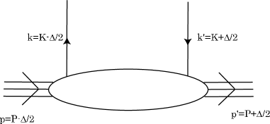
Figure 1: Soft amplitude for the GPDs.

In hard exclusive processes, a high energy virtual photon of momentum $q^{\mu}$ is absorbed by a quark in a nucleon, producing a real photon or a meson and without breaking up the nucleon [8, 9, 10]. It is customary to choose a frame where the averaged nucleon four-momentum $P=(p+p^{\prime})/2$ and $q^{\mu}$ are collinear along the z-axis [4]. Then the GPDs $H(x,\xi,\Delta^{2})$ and $E(x,\xi,\Delta^{2})$ are formally given by the leading twist (twist-two) part of the following amplitude

$$\frac{P_{-}}{2\pi}\int dy_{+}e^{ixP_{-}y_{+}}<p^{\prime}\lambda^{\prime}|{\bar{\psi}}^{q}(-y/2)\gamma^{+}\psi^{q}(y/2)|p\lambda>_{y_{-}=\vec{y}_{\perp}=0}$$

$$= {\bar{u}}_{N}(p^{\prime},\lambda^{\prime})\left[H^{q}(x,\xi,\Delta^{2})\gamma^{+}+E^{q}(x,\xi,\Delta^{2})\frac{i\sigma^{+\nu}\Delta_{\nu}}{2M_{N}}\right]u_{N}(p,\lambda)+\cdot\cdot\cdot,$$

where $\Delta=p^{\prime}-p$, superscript $q$ denotes the quark flavor, $|p\lambda>$ stands for a nucleon state with momentum $p$ and helicity $\lambda$, and the meaning of $x$ and $\xi$ will be made clear in the momentum representation below. The ellpsis $(\cdot\cdot\cdot)$ denotes the higher-twist contributions. In momentum space the above expression can be written as

$${\bar{u}}_{N}(p^{\prime},\lambda^{\prime})\left[H^{q}(x,\xi,\Delta^{2})\gamma^{+}+E^{q}(x,\xi,\Delta^{2})\frac{i\sigma^{+\nu}\Delta_{\nu}}{2M_{N}}\right]u_{N}(p,\lambda),$$ (3.17)

$$= \int\frac{d^{4}K}{(2\pi)^{4}}\delta(x-K^{+}/P^{+})tr[\gamma^{+}\chi_{qN}(p,p^{\prime},K)]$$

where $k=(x+\xi)P^{+}$ and $k^{\prime}=(x-\xi)P^{+}$ are respectively the initial and final quark momenta, $K=(k+k^{\prime})/2$, and $\chi_{qN}(p,p^{\prime},K)_{ji}=\int d^{4}ye^{iK\cdot y}<p^{\prime}\lambda^{\prime}|{\bar{\psi}}_{i}(-y/2)\psi_{j}(y/2)|p\lambda>$ is the quark-nucleon scattering amplitude. The LC momentum fraction $x$ and the skewness $\xi$ are given by $x\equiv K^{+}/P^{+}$ and $\xi\equiv-\Delta^{+}/(2P^{+})$, with

$$0<\xi<\sqrt{\frac{-\Delta^{2}}{4M_{N}^{2}-\Delta^{2}}}<1.$$ (3.18)

Due to the on-shell conditions, $p^{2}=p^{\prime 2}=M_{N}^{2}$, we also have:

$$\Delta^{2}=-\frac{4\xi^{2}M_{N}^{2}+\vec{\Delta}_{\perp}^{2}}{1-\xi^{2}}$$ (3.19)

.

It is then clear that a GPD describes the amplitude of emitting a parton with momentum fraction $x+\xi$ in a nucleon and reabsorbing one with momentum fraction $x-\xi$. If $x>\xi$, both the emitted and absorbed partons are quarks; if $x<-\xi$ then both are antiquarks. Finally, if $|x|<\xi$, the two partons involved are a quark-qntiquark pair. From this physical picture, it is clear that, in the forward scattering limit $\xi=0$, GPDs reduce back to the familiar parton distributions $q(x)$:

$$q(x)=H^{q}(x,0,0).$$ (3.20)

Furthermore, by integrating $H^{q}(x,\xi,\Delta^{2})$ over $x$, we recover the nucleon elastic form factors:

$$\int_{-1}^{1}dxH^{q}(x,\xi,\Delta^{2})=F_{1}^{q}(\Delta^{2})$$ (3.21)

$$\int_{-1}^{1}dxE^{q}(x,\xi,\Delta^{2})=F_{2}^{q}(\Delta^{2}).$$ (3.22)

In the NJL model, the GPDs can be calculated by evaluating the Feynman diagrams shown in Fig. 2, where the contributions from the quark and diquark currents, $J^{Q}_{\lambda^{\prime},\lambda}(x,\xi,\Delta^{2})$ and $J^{D}_{\lambda^{\prime},\lambda}(x,\xi,\Delta^{2})$, are shown separately. Note that in the NJL model we use here, only the isoscalar diquark is considered, then it is easy to see that:

$$J^{u}_{\lambda^{\prime},\lambda}(x,\xi,\Delta^{2}) = J^{Q}_{\lambda^{\prime},\lambda}(x,\xi,\Delta^{2})+J^{D}_{\lambda^{\prime},\lambda}(x,\xi,\Delta^{2}),$$ (3.23)

$$J^{d}_{\lambda^{\prime},\lambda}(x,\xi,\Delta^{2}) = J^{D}_{\lambda^{\prime},\lambda}(x,\xi,\Delta^{2}),$$ (3.24)

where superscript $Q(D)$ denotes the quark (diquark) current contribution. We further write ($X=Q,D$)

$$J^{X}_{\lambda^{\prime},\lambda}(x,\xi,\Delta^{2})\equiv{\bar{u}}_{N}(p^{\prime},\lambda^{\prime})\left[H^{X}(x,\xi,\Delta^{2})\gamma^{+}+E^{X}(x,\xi,\Delta^{2})\frac{i\sigma^{+\nu}\Delta_{\nu}}{2M_{N}}\right]u_{N}(p,\lambda).$$ (3.25)

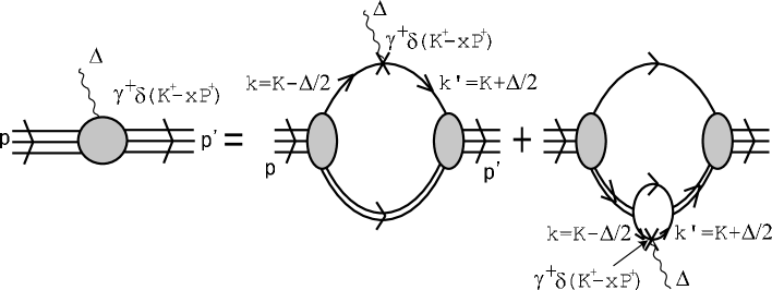
Figure 2: Graphical representation of the quark GPDs of the nucleon. The single (double) line denotes the constituent quark propagator (diquark t-matrix). The operator insertion stands for $\gamma^{+}\delta(K_{-}-xP_{-})(1\pm\tau_{z})/2$ for the u(d) quark. Initial (final) nucleon momentum and helicity are denoted as $p$ ($p^{\prime}$) and $\lambda$ ($\lambda^{\prime}$), and the four-momentum transfer is given by $\Delta^{\mu}=p^{\prime\mu}-p^{\mu}$.

Using the table of matrix elements listed in Appendix A, we can separate the left hand side of Eq. (3) into helicity conserving and helicity flipping contributions:

$$J^{X}_{\lambda^{\prime},\lambda}(x,\xi,\Delta^{2})=\frac{P^{+}}{M_{N}}{\bar{u}}_{N}(p^{\prime},\lambda^{\prime})u_{N}(p,\lambda)$$

$$\times \left[\delta_{\lambda^{\prime},\lambda}\left((1-\xi^{2})H^{X}(x,\xi,\Delta^{2})-\xi^{2}E^{X}(x,\xi,\Delta^{2})\right)-\delta_{\lambda^{\prime},-\lambda}E^{X}(x,\xi,\Delta^{2})\right]$$

In the following we shall only give an outline of the calculations, and leave the details to Appendices B and C.

Using simple Feynmann rules, we can directly read off the quark current contribution $J^{Q}_{\lambda^{\prime},\lambda}(x,\xi,\Delta^{2})$ from Fig. 2,

$$J^{Q}_{\lambda^{\prime},\lambda}(x,\xi,\Delta^{2})=-Z_{N}{\bar{u}}_{N}(p^{\prime},\lambda^{\prime})\int\frac{d^{4}K}{(2\pi)^{4}}\delta\left(x-\frac{K^{+}}{P^{+}}\right)S(k^{\prime})\gamma^{+}S(k)\tau_{D}(p-k)u_{N}(p,\lambda)\\ ,$$ (3.27)

where $\tau_{D}$ is the reduced t-matrix of the diquark. $\tau_{D}$ can be decomposed into two terms:

$$\tau_{D}=\tau_{D}^{C}+\tau_{D}^{P}$$ (3.28)

where $\tau_{D}^{C}$ and $\tau_{D}^{P}$ are respectively the ”contact” and ”pole” contributions, as given in Eq. (2.5) Accordingly, the quark current contribution $J^{Q}$ can also be separated into two terms:

$$J^{Q}_{\lambda^{\prime},\lambda}(x,\xi,\Delta^{2})=\theta(-\xi<x<\xi)J^{Q,C}_{\lambda^{\prime},\lambda}(x,\xi,\Delta^{2})+\theta(-\xi<x<1)J^{Q,P}_{\lambda^{\prime},\lambda}(x,\xi,\Delta^{2}),$$ (3.29)

where we see that $J^{Q,C}$ contributes only in the region $-\xi<x<\xi$, while $J^{Q,P}$ only in $-\xi<x<1$. Thus we see that, unlike other calculations using non-relativistic quark models, the field theoretic NJL model gives a non-zero contribution in the $-\xi<x<1$ region.

Our final expressions for the $H_{Q}$ and $E_{Q}$ are given in Eqs. (B) and (LABEL:E_Q).

Similarly, we can also write down the diquark current contribution,

$$J^{D}_{\lambda^{\prime},\lambda}(x,\xi,\Delta^{2})=-Z_{N}{\bar{u}}(p^{\prime},\lambda^{\prime})\int\frac{d^{4}T}{(2\pi)^{4}}iS(P-T)\tau_{D}(t^{\prime})\tau_{D}(t)$$

$$\times i\int\frac{d^{4}K}{(2\pi)^{4}}tr\left[\gamma^{5}C\tau_{2}\beta_{A}S(k^{\prime})\gamma^{+}S(k)C^{-1}\gamma^{5}\tau_{2}\beta_{A}S(t-k)^{T}\right]\delta\left(x-\frac{K_{-}}{P_{-}}\right)u(p,\lambda),$$

where $t=T-\Delta/2,t^{\prime}=T+\Delta/2$ are the diquark momenta.

We define two additional LC momentum fractions $y,z$,

$$y\equiv K^{+}/T^{+},~{}~{}z\equiv T^{+}/P^{+},$$ (3.31)

so that

$$\int dy\int dz\delta\left(y-\frac{K^{+}}{T^{+}}\right)\delta\left(z-\frac{T^{+}}{P^{+}}\right)=1.$$ (3.32)

Inserting Eq. (3.32) into Eq. (LABEL:Diquark_current), we can rewrite the diquark current contribution in a convolution form:

$$J^{D}_{\lambda^{\prime},\lambda}(x,\xi,\Delta^{2})=\int\frac{d^{4}T}{(2\pi)^{4}}\int dy\int dz\delta(x-yz){\cal F}^{D/N}_{\lambda^{\prime},\lambda}(z,\xi,T,\Delta)$$ (3.33)

$$\times \left(F^{D}_{s}(y,\zeta,T,\Delta)T^{+}+F^{D}_{a}(y,\zeta,T,\Delta)\Delta^{+}\right),$$

with

$$\left(F^{D}_{s}(y,\zeta,T,\Delta)T^{+}+F^{D}_{a}(y,\zeta,T,\Delta)\Delta^{+}\right)$$

$$= ig_{D}^{2}\int\frac{d^{4}K}{(2\pi)^{4}}\delta\left(y-\frac{K^{+}}{T^{+}}\right)tr\left[\gamma^{5}C\tau_{2}\beta_{A}S(k^{\prime})\gamma^{+}S(k)C^{-1}\gamma^{5}\tau_{2}\beta_{A}S(t-k)^{T}\right],$$

$${\cal F}^{D/N}_{\lambda^{\prime},\lambda}(z,\xi,T,\Delta)=-ig_{D}^{-2}Z_{N}{\bar{u}}(p^{\prime},\lambda^{\prime})\delta\left(z-\frac{T^{+}}{P^{+}}\right)S(P-T)\tau_{D}(t^{\prime})\tau_{D}(t)u(p,\lambda),$$ (3.35)

where $g_{D}$ is given in Eq. (2.6), and $\zeta$ is the skewness defined by the relation $\Delta^{+}=-2\zeta T^{+}$.

From the Ward identity for the diquark-diquark-photon vertex $\Gamma_{D}^{\mu}(T,\Delta)$,

$$\Delta_{\mu}\tau_{D}(t^{\prime})\Gamma_{D}^{\mu}(T,\Delta)\tau_{D}(t)=+2i[\tau_{D}(t^{\prime})-\tau_{D}(t)],$$ (3.36)

we obtain

$$\tau_{D}(t^{\prime})\tau_{D}(t)=\frac{2i[\tau_{D}(t^{\prime})-\tau_{D}(t)]}{\Delta_{\mu}\Gamma_{D}^{\mu}(T,\Delta)}.$$ (3.37)

In order to reduce the complexity of the calculation, we introduce the ’on-shell diquark approximation’, i.e., $t^{2}=t^{\prime 2}=M_{D}^{2}$. Then the vertex $\Gamma_{D}^{\mu}$ can be expressed in terms of a single form factor $G_{s}^{D}$

$$\Gamma_{D}^{\mu}(T,\Delta)\simeq G_{s}^{D}(\Delta^{2})T^{\mu}.$$ (3.38)

(see Appendix C for details).

Using Eqs. (2.5) and (3.38), we can rewrite Eq. (3.37) as

$$\tau_{D}(t^{\prime})\tau_{D}(t)\rightarrow\frac{-g_{D}^{2}}{G_{s}^{D}(\Delta^{2})(t^{\prime 2}-M_{D}^{2})(t^{2}-M_{D}^{2})}.$$ (3.39)

Substituting this result into Eq. (3.40), we finally arrive at

$${\cal F}^{D/N}_{\lambda^{\prime},\lambda}(z,\xi,T,\Delta)=iZ_{N}{\bar{u}}(p^{\prime},\lambda^{\prime})\frac{\delta(z-T^{+}/P^{+})S(P-T)}{G_{s}^{D}(\Delta^{2})(t^{\prime 2}-M_{D}^{2})(t^{2}-M_{D}^{2})}u(p,\lambda).$$ (3.40)

The final results for $H^{D}(x,\xi,\Delta^{2})$ and $E^{D}(x,\xi,\Delta^{2})$ are given in Eq. (LABEL:H_D). In Appendix C, apart from $\Delta^{\mu}$, we have introduced another momentum transfer variable $\Delta_{D}^{\mu}$ inside the convolution integral. In a complete evaluation, we should have $\Delta^{\mu}=\Delta_{D}^{\mu}$. However the on-shell diquark approximation gives raise to an ambiguity. In [26], it is assumed that $\Delta^{2}=\Delta_{D}^{2}$ and $\Delta^{+}=\Delta_{D}^{+}$, then $\zeta=\xi/z$. This form is adopted for small $\xi$ and $\vec{\Delta}_{\perp}^{2}<<M_{N}^{2}$. However this choice of $\Delta_{D}^{\mu}$ is not satisfactory in our case, since for $\Delta^{+}=\Delta_{D}^{+}$ implies that the GPDs are non-vanishing only in the region $\xi<z$, and it follows from Eq. (LABEL:sum_rule) that the sum rule is explicitly broken. In order to preserve the sum rule relation, which we believe is important, we let $\vec{\Delta}_{\perp}^{2}=\vec{\Delta}_{D\perp}^{2}$. Then $\zeta$ is fixed by the relation $\Delta^{2}=\Delta_{D}^{2}$ because

$$\Delta^{2}=-\frac{4\xi^{2}M_{N}^{2}+\vec{\Delta}_{\perp}^{2}}{1-\xi^{2}},$$ (3.41)

$$\Delta_{D}^{2}=-\frac{4\zeta^{2}M_{D}^{2}+\vec{\Delta}_{D\perp}^{2}}{1-\zeta^{2}}.$$ (3.42)

Finally we also include the photon-quark vertex correction for the GPDs and electromagnetic form factors which arises from the structure of the constituent quark. Specifically, we sum the series of ring diagrams as shown in Fig. 3. In the spirit of vector dominance, we demand that the resultant photon vertex possesses a pole at $\Delta^{2}=M_{\omega}^{2}~{}(\Delta^{2}=M_{\rho}^{2})$ in the isoscalar (isovector) channel . This effectively replaces the bare vertex $\tau^{a}\gamma^{\mu}$ by

$$\tau^{a}\gamma^{\mu}\rightarrow\frac{\tau^{a}\gamma^{\mu}}{1+2G_{a}\Delta^{2}\Pi_{V,T}(\Delta^{2})},$$ (3.43)

where $a=0(i)$ corresponds to the isoscalar (isovector) part $(\tau^{0}=1)$, and the corresponding coupling constants are $G_{\omega}$ (for $a=0$) and $G_{\rho}$ (for $a=i$). The definition of $\Pi_{V,T}(\Delta^{2})$ and the details of the calculation can be found in appendix D.

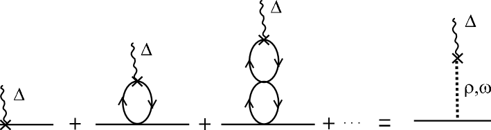
Figure 3: The vector meson dominance corrections to the $\gamma qq$ vertex. The dotted line represents the vector mesons $\omega$ and $\rho$.

As we shall see in the next section, these vertex corrections significantly improve the momentum dependence of the electromagnetic form factors calculated in the NJL model.

4 Results and discussions

In this section, we present the results of our calculation. We shall first explain the choice of parameters in our model. Subsequently, numerical results are presented and compared with those obtained from other works.

In the NJL model we have adopted here, the constituent quark mass is taken to be $M_{Q}=400$ MeV, which is within the range of values used in other works [40]. Using this constituent quark mass, together with the pion mass $m_{\pi}=140$ MeV and the pion decay constant $f_{\pi}=93$ MeV , we can determine the Pauli-Villars cutoff parameter $\Lambda=739$ MeV, the coupling constant $G_{\pi}=10.42$ GeV^-2, and the current quark mass $m_{q}=9$ MeV. Furthermore, we set $G_{s}=0.65G_{\pi}$ so that the solution of the Faddeev equation reproduces the experimental nucleon mass $M_{N}=940$ MeV, the scalar diquark mass is then fixed to be $M_{D}=590$ MeV. Finally, the coupling constants $G_{\omega}=7.34$ GeV^-2 and $G_{\rho}=8.38$ GeV^-2 are determined from the poles of Eq. (D.81), so that the physical vector meson masses $m_{\omega}=783$ MeV and $m_{\rho}=770$ MeV are reproduced.

The nucleon electromagnetic form factors $F_{1}^{p}(\Delta^{2})$ and $F_{1}^{n}(\Delta^{2})$ calculated in the NJL model are depicted in Figs. 4(a) and 4(b), respectively, where results with and without corrections to the photon-quark electromagnetic vertex (see Fig. 3) are shown separately. For comparison, we have also plotted the results corresponding to the familiar ”dipole fit” to the experimental data of $G_{E}$’s and $G_{M}$’s by dashed lines:

$$G_{E}^{p},G_{M}^{p,n} \propto (1-\Delta^{2}/\Delta_{0}^{2})^{-2}$$ (4.44)

$$G_{E}^{n} = 0,$$ (4.45)

with $\Delta_{0}^{2}=0.71$ GeV². We see that the effect of the vertex corrections is rather sizable. In the proton case, where the data are much more precise, inclusion of the vertex correction significantly improves the agreement with experimental data, which is very well parameterized by the “dipole fit”. Nevertheless discrepancies still exist for $-\Delta^{2}>0.5$ GeV². Note that for $\vec{\Delta}_{\perp}=\vec{0}_{\perp}$, $-\Delta^{2}=0.5$ GeV² corresponds to $\xi\simeq 0.35$, and in this work we are only concerned with small $\xi$ ($\leq 0.3$). In the case of the neutron, the effect of the vertex correction is small. Compared with the “dipole fit”, the NJL model result for $F_{1}^{n}(\Delta^{2})$ is similar in magnitude, but opposite in sign. Unfortunately the available data in this case are scattered with large error bars, so that it is not possible to determine which curve fits better.

Similarly, the nucleon form factors $F_{2}^{p,n}(\Delta^{2})$ are plotted in Figs. 5(a) and (b). We see that the NJL model results are significantly different from the dipole fits in the low momentum region $-\Delta^{2}<1$ GeV². As a result, the calculated nucleon magnetic moments (in units of nuclear magneton)

$$\mu^{NJL}_{p}=1.75,~{}~{}~{}\mu^{NJL}_{n}=-0.82,$$ (4.46)

are much smaller than the experimental values

$$\mu^{exp}_{p}=2.79,~{}~{}~{}\mu^{exp}_{n}=-1.91.$$ (4.47)

This will affect the reliability of the $E^{q}(x,\xi,\Delta^{2})$ calculated in this model (see discussions below). It is known that further inclusion of the axial vector diquark channel and the pion cloud are important to improve the results for the magnetic moment [34]. However, these effects are outside the scope of our present investigation of GPDs.

Figure 4: (a) Proton form factor $F_{1}^{p}(\Delta^{2})$. The dotted and solid lines are calculated in the NJL model without and without vertex corrections, respectively, and the dashed line is the dipole fit to the experimental data. (b) Neutron form factor $F_{1}^{n}(\Delta^{2})$ in the same notation as (a).

Figure 5: (a) Proton form factor $F_{1}^{n}(\Delta^{2})$, (b) Neutron form factor $F_{2}^{n}(\Delta^{2})$. Notation same as in Fig. 4.

Figure 6: $H^{u}(x,\xi,\Delta^{2})$ for $\xi=0,0.1,0.3$. The solid lines are NJL model results, and the dashed lines are obtained using the Radyushkin’s ansatz for the input forward quark distributions calculated in NJL model.

Figure 7: $H^{d}(x,\xi,\Delta^{2})$ for $\xi=0,0.1,0.3$. Notation same as in Fig. 6.

Figure 8: $E^{u}(x,\xi,\Delta^{2})$ for $\xi=0,0.1,0.3$. Solid lines show NJL results while the dashed lines give the NJL results multiplied with a factor of $F_{2,EXP}^{u}(\Delta^{2})/F_{2,NJL}^{u}(\Delta^{2})$ (see text for explanation). The dotted line represent $\kappa_{u}u(x)$.

Figure 9: $E^{d}(x,\xi,\Delta^{2})$ for $\xi=0,0.1,0.3$; Notation same as in Fig. 8.

Having fixed the model parameters, we now present the main results of this work. The calculated GPD’s, $H^{u}(x,\xi,\Delta^{2}),H^{d}(x,\xi,\Delta^{2}),E^{u}(x,\xi,\Delta^{2}),$ and $E^{d}(x,\xi,\Delta^{2})$, are plotted in Figs. (6-9), for three different values of $\xi=0,0.1,0.3$, with $\Delta^{2}$ given by Eq. (3.41). For simplicity we have assumed $\vec{\Delta}_{\perp}=\vec{0}_{\perp}$.

As mentioned in Section 3, the quark-current contribution $J^{Q}$ to the GPDs can be decomposed into two terms, $J^{Q,P}$ and $J^{Q,C}$, corresponding respectively to the ”pole-term” and ”contact term” in the diquark t-matrix, see Eq. (3.29). It has been found that the contact term violates PCAC by as much as 13% [36] which is related to the use of ”static approximation” for the Faddeev vertex function. Moreover, the contact term contributes only in the quark-antiquark region, $-\xi<x<\xi$, producing unphysical kinks at $x=\pm\xi$. In view of these facts which indicate that the contact terms can not be assessed reliably in the static approximation, we have chosen to leave out the contact term contribution in our results.

Like all constituent quark models, there are no intrinsic anti-quarks in the NJL model, therefore $H^{q}(x,\xi=0,\Delta^{2})$ and $E^{q}(x,\xi=0,\Delta^{2})$ ($q=u,d$) vanish for negative x. However, unlike the constituent quark models, the NJL model is field theoretic in nature and the Fock states with antiquarks can appear in the intermediate states. Accordingly, the quark-antiquark contribution to GPDs in the region $-\xi<x<\xi$ is accessible in our calculation.

As mentioned before, the calculated electromagnetic form factors $F^{p,n}_{2}(\Delta^{2})$ do not reproduce the experimental data in the low momentum transfer region $-\Delta^{2}<1$ GeV². These discrepancies would affect the quality of $E^{q}(x,\xi,\Delta^{2})$ calculated in our model because $F^{q}_{2}(\Delta^{2})$ is related to the first moment of $E^{q}(x,\xi,\Delta^{2})$ through Eq. (3.22). Consequently, we scale up our calculated $E^{q}$ values by a factor of $F^{u,d(exp)}_{2}/F^{u,d(NJL)}_{2}$ and plot them in Figs. 8 and 9.

It is interesting to compare our results with those obtain using Radyushkin’s ansatz [27]. Radyushkin proposed to write the GPD in terms of a “double distribution” $F^{q}(\beta,\alpha,\Delta^{2})$ which is assumed to be factorized:

$$F^{q}(\beta,\alpha,\Delta^{2})=h(\alpha,\beta)q(\alpha)F_{1}^{q}(\Delta^{2})/F_{1}^{q}(0),$$ (4.48)

where $q(x)$ is the forward quark distribution (or quark distribution function) and the profile function $h(\alpha,\beta)$ has the property of asymptotic meson distribution amplitudes given in [27]:

$$h(\alpha,\beta)=\frac{3}{4}\frac{(1-\beta)^{2}-\alpha^{2}}{(1-\beta)^{3}}.$$ (4.49)

$H^{q}(x,\xi,\Delta^{2})$ is then given by the convolution expression:

$$H^{q}(x,\xi,\Delta^{2})=\int_{-1}^{1}d\beta\int_{-1+|\beta|}^{1-|\beta|}d\alpha\delta(x-\beta-\alpha\xi)F^{q}(\beta,\alpha,\Delta^{2}).$$ (4.50)

Using the forward quark distributions calculated in the NJL model as input, we plot the results obtained from the above ansatz also in Fig. 6 and Fig. 7. We see that, in magnitudes and in shapes, Radyushkin’s ansatz gives qualitatively similar results as the NJL model. One visible quantitative difference is that, as $\xi$ increases, the peak position of $H^{q}(x,\xi,\Delta^{2})$ shifts towards larger $x$ in the NJL model, while it stays almost unchanged in the Radyushkin’s ansatz.

In Figs. (8-9), $\kappa_{q}=F^{q}_{2}(0)$. It is seen that $\kappa_{d}d(x)$ is quite similar to $E^{d}(x,\xi=0,\Delta^{2}=0)$. This is because $E^{d}$ receives contribution only from the diquark current in our model. On the other hand, our result for $\kappa_{u}u(x)$ is rather different from $E^{u}(x,\xi=0,\Delta^{2}=0)$, in contrast to the results obtained with the chiral quark-soliton model [21] and constituent quark models [25, 26].

Figure 10: (a) $H^{u}(x,\xi,\Delta^{2})$ for $\xi=0,0.1,0.3$. The solid lines are the NJL model results and the dashed lines are obtained with constituent quark models [43]. (b) $H^{d}(x,\xi,\Delta^{2})$ for $\xi=0,0.1,0.3$. Notation same as in (a).

Figure 11: (a) $E^{u}(x,\xi,\Delta^{2})$ for $\xi=0,0.1,0.3$. (b) $E^{d}(x,\xi,\Delta^{2})$ for $\xi=0,0.1,0.3$. Notation same as in Fig. 10.

In Figs. (10-11), we compare our results with those obtained in a calculation using the constituent quark model [43] which is calculated using a simple gaussian wave function. We note that their calculation of GPDs is exactly same as [25] except the use of a different wave function. First of all, we see that the signs of the GPDs calculated in the two models agree except $E^{u}(x,\xi,\Delta^{2})$, that is, $E^{u}(x,\xi,\Delta^{2})$ calculated in the NJL model explicitly shows a negative contribution for small $x$. Secondly we see that the shifting of the peak positions towards larger $x$ with increasing $\xi$ are common in both calculations. Finally, we observe that due to the fact that there is no quark-antiquark contribution to the GPDs in the constituent quark model, the curves all terminate at $x=\xi$. In contrast, as mentioned earlier, the NJL model is field theoretic in nature, so that quark-antiquark contributions is non-zero in our calculation. As a result, the range of validity is $-\xi<x<1$ in our calculation.

Comparing our results with those obtained from the chiral quark-soliton model [21, 40], we find that the behavior in the range $-\xi<x<\xi$ is quite different. In the case of chiral quark-soliton model, strong oscillatory behavior is seen around $x=\pm\xi$, whereas our results are rather smooth. This difference arises from the fact that in the chiral quark-soliton model, there is a so called ”d-term” contribution [9, 41, 42] which corresponds to the case where the active quark and antiquark are correlated in the scalar isoscalar (or $\sigma$) channel [24]. Such a contribution is supported by the recent preliminary HERMES data [44] on beam-charge asymmetry in DVCS but is not included in our model.

5 Summary

In this work, we have calculated the spin-averaged ($H^{q}$) and helicity-flip ($E^{q}$) GPDs of the proton, using the NJL model based on a relativistic Faddeev approach with ”static approximation”. The NJL model is a field theoretic approach which has been successfully used in the studies of the static properties and parton distribution functions of the nucleon. Hence the NJL model provides a reasonable framework in which to calculate the GPDs or off-forward parton distribution functions. Among other things, there are two major advantages of adopting this model. First, due to the fact that NJL model is a relativistic field theoretic model Fock states with anti-quarks can exist in the intermediate states, hence quark-antiquark contributions to the GPDs in the region $-\xi<x<\xi$ are non-vanishing. In addition, the model independent sum rules relating the GPDs and nucleon electromagnetic form factors are satisfied.

The calculated GPDs are qualitatively similar to those calculated with the Radyushkin’s double distribution ansatz with forward parton distribution functions calculated in the NJL model as inputs. Comparing our results with those obtained in constituent quark models [25, 26], we find that the general features are similar, except for the fact that the region $-\xi<x<\xi$ is not accessible in the latter.

In our present treatment of the NJL model, as well as in other quark models, configurations with intrinsic antiquarks are not present. Hence it is not possible to investigate GPDs in the region $x<-\xi$. In our case, antiquark contribution can be studied if we include the pion cloud surrounding the three-quark core. In addition, since NJL model is an effective quark theory in the low energy regime, we need to evolve our results, according to perturbative QCD, in order to compare them with data taken in high-energy experiments. Such an NLO $Q^{2}$-evolution of the calculated GPDs, from the low-momentum scale to the experimental one, has been carried in Refs. [26, 45]. We will leave these improvements to future investigations.

Appendix A Matrix elements of Dirac spinors

Table 1 contains the matrix elements of Dirac spinors used in our calculations [39]. The convention of [39] is adopted here:

$$u_{N}(p,\lambda) = \frac{1}{\sqrt{\sqrt{2}p^{+}}}(\sqrt{2}p^{+}+\vec{\alpha}_{\perp}\cdot\vec{p}_{\perp}+\beta M_{N})\chi(\lambda),$$ (A.51)

$$\chi(+1) = \frac{1}{\sqrt{2}}\left(\begin{array}[]{c}1\\ 0\\ 1\\ 0\\ \end{array}\right),\,\,\,\chi(-1)=\frac{1}{\sqrt{2}}\left(\begin{array}[]{c}0\\ 1\\ 0\\ -1\\ \end{array}\right);$$ (A.60)

and $a_{\perp}(\lambda)$ and $a_{\perp}\land b_{\perp}$ are defined by

$$a_{\perp}(\lambda)\equiv\lambda a^{1}+ia^{2},\,\,\,a_{\perp}\land b_{\perp}\equiv a^{1}b^{2}-a^{2}b^{1}.$$ (A.61)

Table 1: Matrix elements of Dirac spinors ${\bar{u}}_{N}(p^{\prime},\lambda^{\prime}){\cal M}u_{N}(p,\lambda)$

${\cal M}$	$\frac{\delta_{\lambda^{\prime},\lambda}}{\sqrt{p^{\prime+}p^{+}}}{\bar{u}}_{N}(p^{\prime},\lambda^{\prime}){\cal M}u_{N}(p,\lambda)$	$\frac{\delta_{\lambda^{\prime},-\lambda}}{\sqrt{p^{+}p^{\prime+}}}{\bar{u}}_{N}(p^{\prime},\lambda^{\prime}){\cal M}u_{N}(p,\lambda)$
1	$\frac{M_{N}}{p^{\prime+}}+\frac{M_{N}}{p^{+}}$	$\frac{p^{\prime}_{\perp}(\lambda)}{p^{\prime+}}-\frac{p_{\perp}(\lambda)}{p^{+}}$
$\gamma^{+}$	2	0
$\gamma^{-}$	$\frac{1}{p^{\prime+}p^{+}}(\vec{p^{\prime}}_{\perp}\cdot\vec{p}_{\perp}+M_{N}^{2}+i\lambda p^{\prime}_{\perp}\land p_{\perp})$	$\frac{M_{N}}{p^{\prime+}p^{+}}(p^{\prime}_{\perp}(\lambda)-p_{\perp}(\lambda))$
$\vec{\gamma}_{\perp}\cdot\vec{a}_{\perp}$	$\vec{a}_{\perp}\cdot\left(\frac{p^{\prime}_{\perp}}{p^{\prime+}}+\frac{p_{\perp}}{p^{+}}\right)-i\lambda a_{\perp}\land\left(\frac{p^{\prime}_{\perp}}{p^{\prime+}}-\frac{p_{\perp}}{p^{+}}\right)$	$-a_{\perp}(\lambda)\left(\frac{M_{N}}{p^{\prime+}}-\frac{M_{N}}{p^{+}}\right)$
$\gamma^{-}\gamma^{+}$	$\frac{2}{p^{\prime+}}M_{N}$	$\frac{2}{p^{\prime+}}p^{\prime}_{\perp}(\lambda)$
$\vec{\gamma}_{\perp}\cdot\vec{a}_{\perp}\gamma^{+}$	0	$2a_{\perp}(\lambda)$
$\gamma^{-}\gamma^{+}\gamma^{-}$	$\frac{2}{p^{\prime+}p^{+}}(\vec{p^{\prime}}_{\perp}\cdot\vec{p}_{\perp}+M_{N}^{2}+i\lambda p^{\prime}_{\perp}\land p_{\perp})$	$\frac{2}{p^{\prime+}p^{+}}(p^{\prime}_{\perp}(\lambda)-p_{\perp}(\lambda))$
$\gamma^{-}\gamma^{+}\vec{\gamma}_{\perp}\cdot\vec{a}_{\perp}$	$\frac{2}{p^{\prime+}}(\vec{a}_{\perp}\cdot\vec{p^{\prime}}_{\perp}-i\lambda a_{\perp}\land p^{\prime}_{\perp})$	$-\frac{2M_{N}}{p^{\prime+}}a_{\perp}(\lambda)$
$\gamma^{+}\gamma^{-}\vec{\gamma}_{\perp}\cdot\vec{a}_{\perp}$	$\frac{2}{p^{+}}(\vec{a}_{\perp}\cdot\vec{p}_{\perp}+i\lambda a_{\perp}\land p_{\perp})$	$\frac{2M_{N}}{p^{+}}a_{\perp}(\lambda)$
$\vec{a}_{\perp}\cdot\vec{\gamma}_{\perp}\gamma^{+}\vec{b}_{\perp}\cdot\vec{\gamma}_{\perp}$	$2(\vec{a}_{\perp}\cdot\vec{b}_{\perp}+i\lambda a_{\perp}\land b_{\perp})$	0

Appendix B Quark current contribution

In Eq. (3.27), the $K^{+}$-integral can be trivially performed. Then with the help of table 1, we get

$${\bar{u}}_{N}(p^{\prime},\lambda^{\prime})(\mbox{$\!\not\!k^{\prime}$}+M)\gamma^{+}(\mbox{$\!\not\!k$}+M)u_{N}(p,\lambda)$$

$$= {\bar{u}}_{N}(p^{\prime},\lambda)u_{N}(p,\lambda)\frac{P^{+}}{M_{N}}\left[(x^{2}-\xi^{2})M_{N}^{2}+(2x+\xi-\xi^{2})MM_{N}-\frac{(1-x)^{2}}{4}\vec{\Delta}_{\perp}^{2}\right.$$

$$+(1-\xi^{2})(\vec{K}_{\perp}^{2}+M^{2})\left.+(1+x+\xi+\xi^{2})\vec{K}_{\perp}\cdot\vec{\Delta}_{\perp}+i\lambda(1+2\xi+x){K}_{\perp}\land{\Delta}_{\perp}\right]$$

$$(\mbox{for $\lambda^{\prime}=\lambda$})$$

$$= {\bar{u}}_{N}(p^{\prime},-\lambda)u_{N}(p,\lambda)\frac{P^{+}}{M_{N}}\left[2(1-x)M_{N}\left((x+2\xi\frac{K_{\perp}(\lambda)}{\Delta_{\perp}(\lambda)})M_{N}+M\right)\right]$$

$$(\mbox{for $\lambda^{\prime}=-\lambda$})$$

The rest of Eq. (3.27)is given by

$$-Z_{N}\int\frac{d^{2}K_{\perp}}{(2\pi)^{4}}dK^{-}\frac{\tau_{D}^{C}(p-k)+\tau_{D}^{P}(p-k)}{(k^{\prime 2}-M^{2})(k^{2}-M^{2})}.$$ (B.62)

After performing the $K^{-}$-integral, we obtain

$$\int dK^{-}\frac{-\tau_{D}^{C}(p-k)}{(k^{\prime 2}-M^{2})(k^{2}-M^{2})}\equiv F_{C}(x,\xi,\vec{K}_{\perp},\vec{\Delta}_{\perp},M^{2},M_{D}^{2})$$

$$= \frac{-4G_{s}\theta(-\xi<x<\xi)}{B_{Q}(x,\xi,\vec{K}_{\perp},\vec{\Delta}_{\perp},M^{2},M_{D}^{2})},$$

$$\int dK^{-}\frac{-\tau_{D}^{P}(p-k)}{(k^{\prime 2}-M^{2})(k^{2}-M^{2})}\equiv F_{P}(x,\xi,\vec{K}_{\perp},\vec{\Delta}_{\perp},M^{2},M_{D}^{2})$$

$$= \frac{g_{D}^{2}}{2A_{Q}(x,-\xi,\vec{K}_{\perp},-\vec{\Delta}_{\perp},M^{2},M_{D}^{2})}$$

$$\times \left(\frac{(1-x)\theta(x>\xi)}{A_{Q}(x,\xi,\vec{K}_{\perp},\vec{\Delta}_{\perp},M^{2},M_{D}^{2})}+\frac{(x+\xi)\theta(-\xi<x<\xi)}{B_{Q}(x,\xi,\vec{K}_{\perp},\vec{\Delta}_{\perp},M^{2},M_{D}^{2})}\right),$$

where

$$A_{Q}(x,\xi,\vec{K}_{\perp},\vec{\Delta}_{\perp},M^{2},M_{D}^{2}) = (1-x)(x-\xi)(1+\xi)P^{2}-(x-\xi)(\vec{K}_{\perp}^{2}+M_{D}^{2})$$

$$-(1-x)[(\vec{K}_{\perp}+\frac{\vec{\Delta}_{\perp}}{2})^{2}+M^{2}],$$

$$B_{Q}(x,\xi,\vec{K}_{\perp},\vec{\Delta}_{\perp},M^{2})=2\left[\xi(x^{2}-\xi^{2})P^{2}-\xi(\vec{K}_{\perp}^{2}+M^{2}+\frac{\Delta_{\perp}^{2}}{4})-x\vec{K}_{\perp}\cdot\vec{\Delta}_{\perp}\right].$$

Combining the above results and with the help of Eq. (LABEL:helicity_relation), we arrive at the final expressions for $H^{Q}$ and $E^{Q}$ which can be decomposed into the ’pole’ and ’contact’ term contributions (Eq. (3.29)): $H^{Q}=H^{C}+H^{P},E^{Q}=E^{C}+E^{P}$. In the following we will explicitly write down the results of $H^{C,P}$ and $E^{C,P}$ with PV regularization scheme (Eq. (2.7)):

$$H^{C,P}(x,\xi,\Delta^{2})$$

$$= \sum_{i}c_{i}\int\frac{d^{2}K_{\perp}}{(2\pi)^{3}}\Biggr{\{}\left[x^{2}-\xi^{2}+2\xi^{2}(1-x)\left(x+2\xi\frac{K_{\perp}(\lambda)}{\Delta_{\perp}(\lambda)}\right)\right]M_{N}^{2}+2x(1-\xi^{2})MM_{N}$$

$$-\frac{(1-x)^{2}}{4}\vec{\Delta}_{\perp}^{2}+(1-\xi^{2})(\vec{K}_{\perp}^{2}+M_{i}^{2})+(1+x+\xi+\xi^{2})\vec{K}_{\perp}\cdot\vec{\Delta}_{\perp}\Biggr{\}}$$

$$\times \frac{F_{C,P}(x,\xi,\vec{K}_{\perp},\vec{\Delta}_{\perp},M_{i}^{2},{M_{D}}_{i}^{2})}{(1-\xi^{2})},$$

$$E^{C,P}(x,\xi,\Delta^{2})$$

$$= \sum_{i}c_{i}\int\frac{d^{2}K_{\perp}}{(2\pi)^{3}}2(1-x)M_{N}\left[\left(x+2\xi\frac{K_{\perp}(\lambda)}{\Delta_{\perp}(\lambda)}\right)M_{N}+M\right]F_{C,P}(x,\xi,\vec{K}_{\perp},\vec{\Delta}_{\perp},M_{i}^{2},{M_{D}}_{i}^{2}),$$

where $M_{i}^{2}=M^{2}+\Lambda_{i}^{2}$, $M_{Di}^{2}=M_{D}^{2}+\Lambda_{i}^{2}$ and the $c_{i}$’s are given in Eq. (2.7) and Eq. (2.9).

Appendix C Diquark current contribution

The diquark current contribution is given in Eq. (LABEL:F_D). In order to simply the calculation, we shall assume the initial and final diquarks are on shell, that is, $t^{\prime 2}=t^{2}=M_{D}^{2}$. Then $T\cdot\Delta_{D}=0$, and $T^{2}=M_{D}^{2}-\Delta_{D}^{2}/4$. In the above and later discussions we will explicitly distinguish $\Delta^{\mu}$ and $\Delta_{D}^{\mu}$, since under the on-shell diquark approximation the frame where we calculate diquark GPDs is not necessarily the same as the one originally chosen for the nucleon GPDs, so that in general $\Delta^{\mu}\neq\Delta_{D}^{\mu}$. Thus, Eq. (LABEL:F_D) becomes

$$\left(F^{D}_{s}(y,\zeta,\Delta_{D}^{2})T^{+}+F^{D}_{a}(y,\zeta,\Delta_{D}^{2})\Delta^{+}\right)$$ (C.66)

$$= ig_{D}^{2}\int\frac{d^{4}K}{(2\pi)^{4}}\delta\left(y-\frac{K^{+}}{T^{+}}\right)tr\left[S(k^{\prime})\gamma^{+}S(k)S(T-K)\right],$$

where $\Delta_{D}^{+}=-2\zeta T^{+}$, and in the frame where $\vec{T}_{\perp}=\vec{0}_{\perp}$, $\Delta_{D}^{2}$ is given by $\Delta_{D}^{2}=-\frac{4\zeta^{2}M_{D}^{2}+\vec{\Delta}_{D\perp}^{2}}{1-\zeta^{2}}$.

Integrating Eq. (C.66) over $y$, we can reproduce the diquark form factors $G_{s,a}^{D}$,

$$\int_{-1}^{1}dyF^{D}_{s,a}(y,\zeta,\Delta_{D}^{2})=G_{s,a}^{D}(\Delta_{D}^{2}),$$ (C.67)

where we see that $G_{s,a}^{D}(\Delta_{D}^{2})$ is independent of $\zeta$ as required. Furthermore for on-shell diquarks, due to the symmery under the exchange of $t$ and $t^{\prime}$, we explicitly find that $G_{a}^{D}(\Delta_{D}^{2})=0$.

After integrating over $K^{+}$ and $K^{-}$, we obtain

$$\left(F^{D}_{s}(y,\zeta,\Delta_{D}^{2})-2\zeta F^{D}_{a}(y,\zeta,\Delta_{D}^{2})\right)T^{+}$$

$$= 6g_{D}^{2}\sum_{i}c_{i}\int\frac{d^{2}K_{\perp}}{(2\pi)^{3}}\Bigg{[}$$

$$\theta(y>\zeta)\frac{\zeta^{2}(1-y)^{2}T^{2}+(1-\zeta^{2})(\vec{K}_{\perp}^{2}+M_{i}^{2})+\frac{(1-y)^{2}\Delta_{D}^{2}}{4}+\zeta(1-y)\vec{K}_{\perp}\cdot\vec{\Delta}_{D\perp}}{A_{D}(y,\zeta,\vec{K}_{\perp},\vec{\Delta}_{D\perp},M_{i}^{2})A_{D}(y,-\zeta,\vec{K}_{\perp},-\vec{\Delta}_{D\perp},M_{i}^{2})}$$

$$- \theta(|y|<\zeta)$$

$$\times \frac{(\zeta^{2}(\zeta-y)+y^{2}(1-\zeta))T^{2}+(1+\zeta)(\vec{K}_{\perp}^{2}+M_{i}^{2})+\frac{(1-y)\Delta_{D}^{2}+(\zeta-y)\vec{\Delta}_{D\perp}^{2}}{4}+y\vec{K}_{\perp}\cdot\vec{\Delta}_{D\perp}}{A_{D}(y,\zeta,\vec{K}_{\perp},\vec{\Delta}_{D\perp},M_{i}^{2})B_{D}(y,\zeta,\vec{K}_{\perp},\vec{\Delta}_{D\perp},M_{i}^{2})},$$

with

$$A_{D}(y,\zeta,\vec{K}_{\perp},\vec{\Delta}_{D\perp},M_{i}^{2})$$

$$= (y+\zeta)(y-1)(1-\zeta)T^{2}+(y+\zeta)\vec{K}_{\perp}^{2}-(y-1)(\vec{K}_{\perp}-\frac{\vec{\Delta}_{D\perp}}{2})^{2}+(1+\zeta)M_{i}^{2},$$

$$B_{D}(y,\zeta,\vec{K}_{\perp},\vec{\Delta}_{D\perp},M_{i}^{2})$$

$$= 2\zeta(y-\zeta)T^{2}+\frac{y-\zeta}{y+\zeta}(\vec{K}_{\perp}-\frac{\vec{\Delta}_{D\perp}}{2})^{2}-(\vec{K}_{\perp}+\frac{\vec{\Delta}_{D\perp}}{2})^{2}-\frac{2\zeta}{y+\zeta}M_{i}^{2},$$

where $T^{2}=M_{D}^{2}-\Delta_{D}^{2}/4$.

Next we need to calculate the following integral

$$F_{\lambda^{\prime},\lambda}^{D/N}(z,\xi,\vec{T}_{\perp},\vec{\Delta}_{\perp})$$

$$= \frac{1}{2\pi}\int{dT^{+}dT^{-}}{\cal F}_{\lambda^{\prime},\lambda}^{D/N}(z,\xi,T,\Delta)$$

$$= \frac{ig_{D}^{2}Z_{N}}{2\pi G_{s}^{D}(\Delta^{2})}{\bar{u}}(p^{\prime},\lambda^{\prime})\int dT^{+}dT^{-}\frac{\delta(z-T^{+}/P^{+})S(P-T)}{(t^{\prime 2}-M_{D}^{2})(t^{2}-M_{D}^{2})}u(p,\lambda).$$

Insert the PV-regularization scheme, and following the same steps as indicated in appendix B, we get

$$F_{\lambda^{\prime},\lambda}^{D/N}(z,\xi,\vec{T}_{\perp},\vec{\Delta}_{\perp})=\frac{g_{D}^{2}Z_{N}}{2G_{s}^{D}(\Delta^{2})}{\bar{u}}(p^{\prime},\lambda^{\prime})u(p,\lambda)\sum_{i}c_{i}\Biggr{[}$$

$$\frac{\theta(z>\xi)(1-z)(M+M_{N}-B_{D/N}^{\lambda^{\prime},\lambda}(T^{-}=P^{-}-\frac{\vec{T}_{\perp}^{2}+M_{i}^{2}}{2(1-z)P^{+}},z,\vec{T}_{\perp},\vec{\Delta}_{\perp}))}{A_{D/N}(z,\xi,\vec{T}_{\perp},\vec{\Delta}_{\perp},M_{i}^{2},M_{Di}^{2})A_{D/N}(z,-\xi,\vec{T}_{\perp},-\vec{\Delta}_{\perp},M_{i}^{2},M_{Di}^{2})}$$

$$- \frac{\theta(|z|<\xi)(x+\xi)(M+M_{N}-B_{D/N}^{\lambda^{\prime},\lambda}(T^{-}=\xi P^{-}+\frac{(\vec{T}_{\perp}-\vec{\Delta}_{\perp}/2)^{2}+M_{Di}^{2}}{2(z+\xi)P^{+}},z,\vec{T}_{\perp},\vec{\Delta}_{\perp}))}{A_{D/N}(z,\xi,\vec{T}_{\perp},\vec{\Delta}_{\perp},M_{i}^{2},M_{Di}^{2})C_{D/N}(z,\xi,\vec{T}_{\perp},\vec{\Delta}_{\perp},M_{Di}^{2})}\Biggl{]},$$

with

$$A_{D/N}(z,\xi,\vec{T}_{\perp},\vec{\Delta}_{\perp},M_{i}^{2},M_{Di}^{2})$$

$$= (1-z)(z+\xi)(1-\xi)P^{2}-(z+\xi)(\vec{T}_{\perp}^{2}+M_{i}^{2})-(1-z)((\vec{T}_{\perp}-\vec{\Delta}_{\perp}/2)^{2}+M_{Di}^{2}),$$

$$C_{D/N}(z,\xi,\vec{T}_{\perp},\vec{\Delta}_{\perp},M_{Di}^{2})$$

$$= 2\xi((z^{2}-\xi^{2})P^{2}-\vec{T}_{\perp}^{2}-\vec{\Delta}_{\perp}^{2}/4-M_{Di}^{2})-2z\vec{T}_{\perp}\cdot\vec{\Delta}_{\perp},$$

$$B_{D/N}^{\lambda^{\prime},\lambda}(T^{-},z,\vec{T}_{\perp},\vec{\Delta}_{\perp}))$$

$$= \frac{\delta_{\lambda^{\prime},\lambda}}{2M_{N}}[z(M_{N}^{2}-\vec{\Delta}_{\perp}^{2}/4)+2(1-\xi^{2})T^{-}P^{+}+\xi\vec{T}_{\perp}\cdot\vec{\Delta}_{\perp}-i\lambda T_{\perp}\land\Delta_{\perp}]$$

$$+ \delta_{\lambda^{\prime},-\lambda}M_{N}\left(z+2\xi\frac{T_{\perp}(\lambda)}{\Delta_{\perp}(\lambda)}\right),$$

where $P^{2}=M_{N}^{2}-\Delta^{2}/4$.

With help of Eq. (LABEL:helicity_relation), we finally arrive at

$$H^{D}(x,\xi,\Delta^{2}) = \int dy\int dz\delta(x-yz)\frac{F_{s}^{D}(y,\zeta,\Delta_{D}^{2})-2\zeta F_{a}^{D}(y,\zeta,\Delta_{D}^{2})}{G_{s}^{D}(\Delta^{2})}$$

$$\times\int\frac{d^{2}T_{\perp}}{(2\pi)^{3}}H^{D/N}(z,\xi,\vec{T}_{\perp},\vec{\Delta}_{\perp}),$$

$$E^{D}(x,\xi,\Delta^{2}) = \int dy\int dz\delta(x-yz)\frac{F_{s}^{D}(y,\zeta,\Delta_{D}^{2})-2\zeta F_{a}^{D}(y,\zeta,\Delta_{D}^{2})}{G_{s}^{D}(\Delta^{2})}$$

$$\times\int\frac{d^{2}T_{\perp}}{(2\pi)^{3}}E^{D/N}(z,\xi,\vec{T}_{\perp},\vec{\Delta}_{\perp}),$$

where

$$H^{D/N}(z,\xi,\vec{T}_{\perp},\vec{\Delta}_{\perp})$$

$$= \frac{g_{D}^{2}Z_{N}}{2}\sum_{i}c_{i}\Biggr{[}\frac{\theta(z>\xi)(1-z)}{A_{D/N}(z,\xi,\vec{T}_{\perp},\vec{\Delta}_{\perp})A_{D/N}(z,-\xi,\vec{T}_{\perp},-\vec{\Delta}_{\perp})}$$

$$+ \frac{\theta(|z|<\xi)(z+\xi)}{A_{D/N}(z,\xi,\vec{T}_{\perp},\vec{\Delta}_{\perp})C_{D/N}(z,\xi,\vec{T}_{\perp},\vec{\Delta}_{\perp})}\Biggl{]}\tilde{H}^{D/N}(T_{i}^{-},z,\xi,\vec{T}_{\perp},\vec{\Delta}_{\perp}),$$

$$E^{D/N}(z,\xi,\vec{T}_{\perp},\vec{\Delta}_{\perp})$$

$$= \frac{Z_{N}}{2}\sum_{i}c_{i}\Biggr{[}\frac{\theta(z>\xi)(1-z)}{A_{D/N}(z,\xi,\vec{T}_{\perp},\vec{\Delta}_{\perp})A_{D/N}(z,-\xi,\vec{T}_{\perp},-\vec{\Delta}_{\perp})}$$

$$- \frac{\theta(|z|<\xi)(z+\xi)}{A_{D/N}(z,\xi,\vec{T}_{\perp},\vec{\Delta}_{\perp})C_{D/N}(z,\xi,\vec{T}_{\perp},\vec{\Delta}_{\perp})}\Biggl{]}\tilde{E}^{D/N}(T_{i}^{-},z,\xi,\vec{T}_{\perp},\vec{\Delta}_{\perp}),$$

in which

$$\tilde{H}^{D/N}(T_{i}^{-},z,\xi,\vec{T}_{\perp},\vec{\Delta}_{\perp})$$

$$= \frac{zM_{N}}{1-\xi^{2}}\Biggr{[}(1+\xi^{2})(M+M_{N})-\xi^{2}M_{N}(z+2\xi\frac{K_{\perp}(\lambda)}{\Delta_{\perp}(\lambda)})$$

$$- \frac{z(M_{N}^{2}-\vec{\Delta}_{\perp}^{2}/4)+2(1-\xi^{2})T_{i}^{-}P^{+}+\xi\vec{T}_{\perp}\cdot\vec{\Delta}_{\perp}}{2M_{N}}\Biggl{]},$$

with

$$T_{i}^{-}=\theta(z>\xi)(P^{-}-\frac{\vec{T}_{\perp}^{2}+M_{i}^{2}}{2(1-z)P^{+}})+\theta(|z|<\xi)(\xi P^{-}+\frac{(\vec{T}_{\perp}-\vec{\Delta}_{\perp}/2)^{2}+M_{Di}^{2}}{2(z+\xi)P^{+}}),$$ (C.75)

and

$$\tilde{E}^{D/N}(T_{i}^{-},z,\xi,\vec{T}_{\perp},\vec{\Delta}_{\perp})=zM_{N}\left(M+M_{N}-M_{N}(z+2\xi\frac{K_{\perp}(\lambda)}{\Delta_{\perp}(\lambda)})\right).$$ (C.76)

Note that if we integrate Eq. (LABEL:H_D) over $x$ with $\Delta^{2}=\Delta_{D}^{2}$ and fixed $\zeta$, then we can reproduce the diquark current contributions to the form factors,

$$\int_{-1}^{1}dxH^{D}(x,\xi,\Delta^{2}) = \int_{-\xi}^{1}dz\int\frac{d^{2}T_{\perp}}{(2\pi)^{3}}H^{D/N}(z,\xi,\vec{T}_{\perp},\vec{\Delta}_{\perp})=F_{1}^{D}(\Delta^{2}),$$

$$\int_{-1}^{1}dxE^{D}(x,\xi,\Delta^{2}) = \int_{-\xi}^{1}dz\int\frac{d^{2}T_{\perp}}{(2\pi)^{3}}E^{D/N}(z,\xi,\vec{T}_{\perp},\vec{\Delta}_{\perp})=F_{2}^{D}(\Delta^{2}),$$

where $F^{D}_{i}$ denotes diquark current contributions to the nucleon form factor which are given in Appendix E.

Appendix D Vertex corrections to the photon vertex

The photon vertex correction, as shown in Fig. 2, consists of the sum of a series of ring diagrams. Each diagram on the left side of the diagrams in Fig. 2 is calculated as follows:

$$\tau^{a}\gamma^{\mu}+(-2)G_{a}\Pi_{V}^{\mu\nu}(\Delta)_{ab}\gamma_{\nu}\tau^{b}+(-2)^{2}G_{a}^{2}\Pi_{V}^{\mu\nu}(\Delta)_{ab}\Pi_{V\nu}^{\mu^{\prime}}(\Delta)_{bc}\gamma_{\mu^{\prime}}\tau^{c}+\cdots,$$ (D.78)

where

$$\Pi_{V}^{\mu\nu}(\Delta)_{ab}=6i\delta_{ab}\int\frac{d^{4}k}{(2\pi)^{4}}tr_{D}[S(k)\gamma^{\nu}S(k+\Delta)\gamma^{\mu}].$$ (D.79)

$\Pi_{V}^{\mu\nu}(\Delta)_{ab}$ can be decomposed into the longitudinal and transverse parts:

$$\Pi_{V}^{\mu\nu}(\Delta)_{ab}\equiv\delta_{ab}[(\Delta^{2}g^{\mu\nu}-\Delta^{\mu}\Delta^{\nu})\Pi_{V,T}(\Delta^{2})+\Delta^{\mu}\Delta^{\nu}\Pi_{V,L}(\Delta^{2})].$$ (D.80)

With the use of Ward identity, then it is clear that the transverse part of $\Pi_{V}^{\mu\nu}(\Delta)_{ab}$ does not contribute due to current conservation. Therefore the series can be easily summed:

$$\rightarrow\frac{\tau^{a}\gamma^{\mu}}{1+2G_{a}\Delta^{2}\Pi_{V,T}(\Delta^{2})},$$ (D.81)

where $a=0(i)$ means the isoscalar (isovector) part and $G_{\omega,\rho}$ express the coupling constants in the vector meson channels.

$\Pi_{V,L}(\Delta^{2})$ can be calculated from

$$[(\Delta^{2}g^{\mu\nu}-\Delta^{\mu}\Delta^{\nu})\Pi_{V,T}(\Delta^{2})+\Delta^{\mu}\Delta^{\nu}\Pi_{V,L}(\Delta^{2})]=6i\int\frac{d^{4}k}{(2\pi)^{4}}tr_{D}[S(k)\gamma^{\nu}S(k+\Delta)\gamma^{\mu}].$$ (D.82)

Inserting the PV-regularization factor, and performing the $k$-integrals, we obtain

$$\Pi_{V,T}(\Delta^{2})=\frac{3}{\pi^{2}}\int_{0}^{1}d\alpha\alpha(1-\alpha)\left[\frac{\Lambda^{2}}{M_{Q}^{2}-\alpha(1-\alpha)\Delta^{2}+\Lambda^{2}}-ln\left(1+\frac{\Lambda^{2}}{M_{Q}^{2}-\alpha(1-\alpha)\Delta^{2}}\right)\right].$$

(D.83)

From Eqs. (D.81) and (D.83), we can easily see that there is no vertex correction at $\Delta^{2}=0$, i.e., when the photon is on the mass shell.

Appendix E Nucleon form factors

Nucleon electromagnetic form factors can be calculated in the same way as the GPDs, with the operator $\gamma^{+}(1\pm\tau_{z})/2$ replaced by $\gamma^{\mu}(1\pm\tau_{z})/2$. We introduce Feynmann parameters $z,x_{1,2}$ to combine the denominators of the propagators, and then a Wick rotation is performed to obtain an Euclidean integral. The resulting expressions are given by

$$F_{1}^{C}(\Delta^{2}) = -4Q_{q}G_{s}Z_{N}\sum_{i}c_{i}\int_{-\frac{1}{2}}^{\frac{1}{2}}dz\frac{1}{2}\int_{0}^{\infty}\frac{tdt}{8\pi^{2}}\frac{\frac{t}{2}+(1-4z^{2})\frac{\Delta^{2}}{4}+M_{Qi}^{2}}{[t+M_{Qi}^{2}-(1-4z^{2})\frac{\Delta^{2}}{4}]^{2}}$$

$$F_{2}^{C}(\Delta^{2}) = -4Q_{q}G_{s}Z_{N}\sum_{i}c_{i}\int_{-\frac{1}{2}}^{\frac{1}{2}}dz\frac{1}{2}\int_{0}^{\infty}\frac{tdt}{8\pi^{2}}\frac{2M_{Q}M_{N}}{[t+M_{Qi}^{2}-(1-4z^{2})\frac{\Delta^{2}}{4}]^{2}}$$

$$F_{1}^{Q}(\Delta^{2}) = Q_{q}g_{d}^{2}Z_{N}\sum_{i}c_{i}\int_{0}^{1}dx_{1}\int_{-x_{1}}^{x_{1}}dx_{2}\frac{1}{2}\int_{0}^{\infty}\frac{tdt}{8\pi^{2}}$$

$$\times \frac{(1-x_{1})^{2}M_{N}^{2}+2(1-x_{1})M_{Q}M_{N}+M_{Qi}^{2}+\frac{t}{2}+(x_{1}^{2}-x_{2}^{2})\frac{\Delta^{2}}{4}}{[t+(1-x_{1})M_{Di}^{2}+x_{1}M_{Qi}^{2}-x_{1}(1-x_{1})M_{N}^{2}-(x_{1}^{2}-x_{2}^{2})\frac{\Delta^{2}}{4}]^{3}}$$

$$F_{2}^{Q}(\Delta^{2}) = Q_{q}g_{d}^{2}Z_{N}\sum_{i}c_{i}\int_{0}^{1}dx_{1}\int_{-x_{1}}^{x_{1}}dx_{2}\frac{1}{2}\int_{0}^{\infty}\frac{tdt}{8\pi^{2}}$$

$$\times \frac{2M_{N}x_{1}[M_{N}(1-x_{1})+M_{Q}]}{[t+(1-x_{1})M_{Di}^{2}+x_{1}M_{Qi}^{2}-x_{1}(1-x_{1})M_{N}^{2}-(x_{1}^{2}-x_{2}^{2})\frac{\Delta^{2}}{4}]^{3}}$$

$$F_{1}^{D}(\Delta^{2}) = Q_{d}g_{d}^{2}Z_{N}\sum_{i}c_{i}\int_{0}^{1}dx_{1}\int_{-x_{1}}^{x_{1}}dx_{2}\frac{1}{2}\int_{0}^{\infty}\frac{tdt}{8\pi^{2}}$$

$$\times \frac{2M_{N}(1-x_{1})(x_{1}M_{N}+M_{Q})+\frac{t}{2}}{[t+(1-x_{1})M_{Qi}^{2}+x_{1}M_{Di}^{2}-x_{1}(1-x_{1})M_{N}^{2}-(x_{1}^{2}-x_{2}^{2})\frac{\Delta^{2}}{4}]^{3}}$$

$$F_{2}^{D}(\Delta^{2}) = Q_{d}g_{d}^{2}Z_{N}\sum_{i}c_{i}\int_{0}^{1}dx_{1}\int_{-x_{1}}^{x_{1}}dx_{2}\frac{1}{2}\int_{0}^{\infty}\frac{tdt}{8\pi^{2}}$$

$$\times \frac{-2M_{N}(1-x_{1})[x_{1}M_{N}+M_{Q}]}{[t+(1-x_{1})M_{Qi}^{2}+x_{1}M_{Di}^{2}-x_{1}(1-x_{1})M_{N}^{2}-(x_{1}^{2}-x_{2}^{2})\frac{\Delta^{2}}{4}]^{3}},$$

where C,P,D mean current, pole and diquark current contributions.

References

[1]F. Sabatie, hep-ex/0207016.
[2]V. D. Burkert, hep-ph/0303006.
[3]A.V. Radyushkin, Phys. Rev. D56, 5524 (1996).
[4]X. Ji and J. Osborne, Phys. Rev. D58, 094018 (1998).
[5]J.C. Collins and A. Freund, Phys. Rev. D59, 074009
(1999).
[6]R.L. Jaffe and A.V. Manohar, Nucl. Phys. B337,
507 (1990).
[13]Hermes Collaboration, A. Airapetian et al.,
Phys. Rev. Lett. 87, 182001 (2001).
[14]CLAS Collaboration, S. Stepanyan et al.,
Phys. Rev. Lett. 87, 182002 (2001).
[15]ZEUS Collaboration, C. Adloff et al.,
Phys. Lett. B517, 47 (2001); S. Chekanov et
al., ibid., B573, 46 (2003).
[16]B. A. Mecking, Nucl. Phys. A711, 330c (2002).
[17]K. Rith, Nucl. Phys. A711, 336c (2002).
[18]M. Gockeler et al., Phys. Rev. Lett.
92, 042002 (2004).
[19]X. Ji, W. Melnitchouk, X. Song, Phys. Rev. D56, 5511 (1997).
[20]I.V. Anikin, D. Binosi, R. Medrano, S. Noguera,
and V. Vento, Eur. Phys. J. A 14, 95 (2002).
[21]V.Y. Petrov, P.V. Pobylitsa, M.V. Polyakov,
I. Bornig, K. Goeke and C. Weiss, Phys. Rev. D57,
4325 (1998); M. Penttinen, M.V. Polyakov, and K. Goeke, ibid.62, 014024 (2000).
[22]B.C. Tiburzi and G.A. Miller, Phys. Rev. C64, 065204 (2001).
[23]B.C. Tiburzi and G.A. Miller, Phys. Rev. D65, 074009 (2002).
[24]L. Theussl, S. Noguera, and V. Vento, Eur.
Phys. J. A 20, 483 (2004).
[25]S. Boffi, B. Pasquini and M. Traini, Nucl.
Phys. B649, 243 (2003); ibid.B680, 147
(2004).
[26]S. Scopetta and V. Vento, Eur. Phys.
J. A16, 527 (2003); Phys. Rev. D69, 094004
(2004).