Running Neutrino Masses, Leptonic Mixing Angles and CP-Violating Phases: From $M_{\rm Z}$ to $\Lambda_{\rm GUT}$

Abstract

We derive renormalization group equations for neutrino masses, leptonic mixing angles and CP-violating phases running at energies above the seesaw threshold, both in the Standard Model and in the Minimal Supersymmetric Standard Model extended with three right-handed neutrinos. With these equations, we carry out a systematic study of the radiative correction that may arise to neutrino parameters, via their renormalization group evolution from the electroweak scale ($M_{\rm Z}$) to the scale of Grand Unified theories ($\Lambda_{\rm GUT}$). We study in detail three typically interesting neutrino mass patterns: normal hierarchy, near degeneracy and inverted hierarchy. Magnitudes of possible corrections in each case are carefully investigated. We also emphasize the significance of CP-violating phases in controlling the evolution behavior of all neutrino parameters.

I Introduction

Experimental information on neutrino masses and mixings has opened up a new playground for efforts[1] of a better understanding of the Yukawa couplings in the Standard Model (SM) and its extensions. In the lepton sector, it is conceptually natural to use the elegant seesaw mechanism [2, 3, 4] to give masses to the SM neutrinos. In the most simple version of this mechanism, the dimension 5 neutrino mass term is the low energy relic of some more fundamental theories with very heavy right-handed neutrinos. So in this framework, we often need to relate physics at vastly different energy scales.

The only way to compare the high energy theoretical prediction and the low energy experimental observation is to use renormalization group equations (RGEs). It has been found that corrections arising from renormalization group (RG) evolution can be very significant for leptonic mixing angles and neutrino mass splitting, especially in the case of nearly degenerate left-handed neutrinos. So in principle, the RG correction should not be neglected in the discussion of models suggested at high energy scales. With RGEs derived in Refs.[5, 6, 7], early discussions[8, 9, 10, 11, 12, 13, 14, 15, 16] of the RG running effect are mainly concerned with neutrino mass (or Yukawa coupling) matrices. The evolution of neutrino masses, leptonic mixing angles and possible CP-violating phases is studied by diagonalizing the relevant Yukawa matrices at different energy scales, and the behaviors are discussed in a numerical or semi-analytical way. However, authors of Refs.[17, 18, 19, 20] have also emphasized the significance of RGEs for individual neutrino parameters. Such equations not only make it possible to predict the evolution behavior of each parameter[21, 22, 23, 24], but also can help people appreciate interesting features such as the existence of (pseudo-) fixed points in the evolution of mixing angles and CP-violating phases [14, 16, 17, 25, 26]. The derivation of these equations below the seesaw threshold has been done in Refs.[17, 18, 27, 23]. And based on such equations, a comprehensive study of the RG evolution of neutrino parameters from the electroweak scale to the seesaw threshold has been carried out in Ref.[27].

However, RG corrections above the seesaw threshold sometimes are as important as or even more significant than those below the threshold[8, 15, 28, 29, 30]. Since the physics responsible for neutrino mass generation is more likely to exist at the scale of Grand Unified theories, a systematic study of the RG correction above the seesaw threshold should be necessary. And this is one of our main concerns in this work. In much the same spirit as of Ref.[27], we derive RGEs for individual neutrino parameters running above the seesaw threshold, under the condition that eigenvalues of the Yukawa coupling matrix that connects left- and right-handed neutrinos are hierarchical. The contribution from the largest eigenvalue of this matrix is explicitly shown. By setting this contribution to zero, we can regain RGEs obtained earlier in Refs.[27, 23], which are valid at energies below the seesaw threshold.

The second purpose of this work is to carry out a systematic study of the radiative correction that may arise via the RG evolution in the full energy range from the electroweak scale ($M_{\rm Z}$) to the scale of Grand Unified theories ($\Lambda_{\rm GUT}$). To demonstrate main features of possible corrections, we study in detail three typically allowed neutrino mass patterns: normal hierarchy, near degeneracy and inverted hierarchy.

The paper is organized as follows. We write down full one-loop RGEs for individual neutrino masses, leptonic mixing angles and CP violating phases in Section II, with a brief discussion. Then in Section III, we carry out a systematic study of the correction that may arise during the RG evolution from $M_{\rm Z}$ to $\Lambda_{\rm GUT}$, in theories with the three neutrino mass patterns mentioned above. Section IV is devoted to a Summary.

II Analytical formulae for neutrino parameters running above the seesaw threshold

Extended with three right-handed neutrinos, the Lagrangian giving mass to leptons in the SM is

$$-{\cal L}_{l}=\overline{E_{L}}HY_{l}l_{R}+\overline{E_{L}}H^{c}Y_{\nu}\nu_{R}+\frac{1}{2}\overline{\nu_{R}^{c}}M_{R}\nu_{R}+h.c.;$$ (1)

and in the MSSM is

$$-{\cal L}_{l}=\overline{E_{L}}H_{1}Y_{l}l_{R}+\overline{E_{L}}H_{2}Y_{\nu}\nu_{R}+\frac{1}{2}\overline{\nu_{R}^{c}}M_{R}\nu_{R}+h.c.,$$ (2)

where, $E_{L}$, $l_{R}$ and $\nu_{R}$ denote $SU(2)_{L}$-doublets, right-handed charged leptons and right-handed neutrinos, respectively. Both in Eqs.(1) and (2), the scale of $M_{R}$ is expected to be extremely high, since there is not a protective symmetry. Around this energy scale, mass eigenstates of $M_{R}$ are successively integrated out at their respective masses $\left(M_{1}<M_{2}<M_{3}\right)$, giving rise to a series of effective theories at different energy scales[28]. Then at energies below the lightest right-handed neutrino mass, we obtain the dimension 5 effective mass term for left-handed neutrinos

$$-{\cal L}_{\nu}=-\frac{1}{2}\overline{E_{L}}\Phi\cdot\kappa\cdot\Phi^{T}E_{L}^{c}+h.c.,$$ (3)

where $\kappa$ is the effective Yukawa coupling matrix, and $\Phi$ is $H^{c}$ in the SM but is $H_{2}$ in the MSSM. Since $\kappa$ is calculated from $Y_{\nu}$ and $M_{R}$ by decoupling right-handed neutrinos at successive energy scales, step by step, the relation between $\kappa$ and $Y_{\nu}$, $M_{R}$ is complicated. Only in the most simplified procedure when all right-handed neutrinos are decoupled at a common scale, can we obtain (at that chosen scale) a simple equation because of the tree-level matching condition[28]:

$$\kappa=Y_{\nu}M_{R}^{-1}Y_{\nu}^{T}~{}.$$ (4)

Then, when the Higgs field acquires a non-zero vacuum expectation value $\langle\Phi\rangle=\left(v~{}~{}0\right)^{T}$ during the electroweak symmetry breaking, Eq.(3) yields an effective mass matrix $M_{\nu}=v^{2}\kappa$ for left-handed neutrinos. In the SM, $v\simeq 174$ GeV; and in the MSSM, $v\simeq 174\sin\beta$ GeV.

Since right-handed neutrinos are to be decoupled at their respective thresholds, it will be too complicated to derive RGEs for neutrino parameters between these thresholds. So we shall be less ambitious than solving the whole problem, but shall simplify it by (a) decoupling all right-handed neutrinos at a common scale, which we take to be $M_{3}$, and (b) limiting our derivation only to the case when eigenvalues of $Y_{\nu}$ are hierarchical. Here, assumption (a) can be justified when the RG evolution through right-handed neutrino thresholds is not too dramatic (As has been demonstrated in Refs.[15, 28], this is not always the case). And assumption (b) is also well motivated since in a large class of high energy models considered in literature (such as those based on $U(1)$ symmetry or those base on $SO(10)$ Grand Unified Theories), there is often a certain similarity or even identification between $Y_{\nu}$ and the up-quark Yukawa coupling matrix. Such a similarity of matrices should lead to some likeness between their eigenvalues.

One-loop RGEs for $\kappa$ running from $M_{\rm Z}$ to $M_{1}$ and those for $Y_{\nu}$ and $M_{R}$ running through right-handed neutrino thresholds to $\Lambda_{\rm GUT}$ have been given in Ref.[28]. For readers’ convenience, we have collected a part of them together with those for $Y_{l}$ in Appendix A. To discuss the RG evolution of neutrino parameters in the full energy range from $M_{\rm Z}$ to $\Lambda_{\rm GUT}$, it is convenient to make use of $\kappa$ also at energies above the seesaw threshold[24, 30]. In this energy range, we find from Eqs.(4), (A.8) and (A.9)

$$16\pi^{2}\frac{\rm d\it\kappa}{\rm d\it t}=\alpha_{\kappa}\kappa+N_{\kappa}\kappa+\kappa N_{\kappa}^{T},$$ (5)

where $t=\ln\mu$ with $\mu$ being the energy scale, and details of $\alpha_{\kappa}$ and $N_{\kappa}$ are given in Eq.(A.17) in the Appendix.

For neutrino masses, leptonic mixing angles and CP-violating phases, $\kappa$ is diagonalized by a unitary matrix $U_{\kappa}$:

$$\kappa=U_{\kappa}\kappa^{\prime}U_{\kappa}^{T};\ \ \ \kappa^{\prime}={\rm diag}\left\{k_{1},k_{2},k_{3}\right\},$$ (6)

where $k_{i}$ (for $i=1,2,3$) at $M_{\rm Z}$ are proportional to left-handed neutrino masses : $k_{i}\left(M_{\rm Z}\right)\equiv m_{i}\left(M_{\rm Z}\right)/v^{2}$. At energy scales below $M_{1}$, $Y_{l}$ is always diagonal during the RG evolution, if it is diagonal at the beginning. In such a basis, the leptonic mixing matrix is $U_{\rm MNS}\equiv U_{\kappa}$. However, $Y_{l}$ can not be kept diagonal above the seesaw threshold when Eq.(A.7) is used for its RG evolution. In this case, there is the contribution to $U_{\rm MNS}$ from diagonalizing $H_{l}=Y_{l}Y_{l}^{\dagger}$:

$$H_{l}=U_{l}H_{l}^{\prime}U_{l}^{\dagger};\ \ \ H_{l}^{\prime}={\rm diag}\left\{y_{e}^{2},y_{\mu}^{2},y_{\tau}^{2}\right\},$$ (7)

$$\Longrightarrow U_{\rm MNS}=U_{l}^{\dagger}U_{\kappa}.$$ (8)

For the MNS matrix, a convenient parametrization can be found in Ref.[31]

$$U_{\rm MNS} = \left(\matrix{1&&\cr&c_{y}&s_{y}\cr&-s_{y}&c_{y}}\right)\left(\matrix{c_{z}&&s_{z}\cr&e^{-i\delta}&\cr-s_{z}&&c_{z}}\right)\left(\matrix{c_{x}&s_{x}&\cr-s_{x}&c_{x}&\cr&&1}\right)\left(\matrix{e^{i\rho}&&\cr&e^{i\sigma}&\cr&&1}\right)$$ (9)

$$= \left(\matrix{c_{x}c_{z}&c_{z}s_{x}&s_{z}\cr-c_{y}s_{x}e^{-i\delta}-c_{x}s_{y}s_{z}&c_{x}c_{y}e^{-i\delta}-s_{x}s_{y}s_{z}&c_{z}s_{y}\cr s_{x}s_{y}e^{-i\delta}-c_{x}c_{y}s_{z}&-c_{x}s_{y}e^{-i\delta}-c_{y}s_{x}s_{z}&c_{y}c_{z}}\right)\left(\matrix{e^{i\rho}&&\cr&e^{i\sigma}&\cr&&1}\right)~{},$$ (10)

where $c_{x}\equiv\cos\theta_{x},s_{x}\equiv\sin\theta_{x}$ and so on. The merit of this parametrization is that the Dirac phase $\delta$ does not appear in the neutrinoless double beta decay, while Majorana phases $\rho$ and $\sigma$ do not contribute to the leptonic CP violation in neutrino oscillations. Thus two different types of phases can be separately studied in different types of experiments.

At energies below the seesaw threshold, RGEs for the running of left-handed neutrino masses $\left(m_{1},m_{2},m_{3}\right)$, leptonic mixing angles $\left(\theta_{x},\theta_{y},\theta_{z}\right)$ and CP-violating phases $\left(\delta,\rho,\sigma\right)$ have been derived in Refs.[17, 18, 27, 23]. In order to obtain the same kind of formulae at energies above the seesaw threshold, we also need a parametrization of $Y_{\nu}$. We find that the derivation is most straightforward if $Y_{\nu}$ is parameterized in the diagonal basis of $\kappa$ by $\left(H_{\nu}\equiv Y_{\nu}Y_{\nu}^{\dagger}\right)$:

$$H_{\nu}=U_{\nu}H_{\nu}^{\prime}U_{\nu}^{\dagger};\ \ \ H_{\nu}^{\prime}=y_{\nu}^{2}\cdot{\rm diag}\left\{r_{1}^{2},r_{2}^{2},1\right\}\ ,$$ (11)

where (with $c_{1}=\cos\theta_{1}$,$\ s_{1}=\sin\theta_{1}$ and so on)

$$U_{\nu}=\left(\matrix{e^{i\phi_{1}}&&\cr&e^{i\phi_{2}}&\cr&&1}\right)\left(\matrix{1&&\cr&c_{1}&s_{1}\cr&-s_{1}&c_{1}}\right)\left(\matrix{c_{2}&&s_{2}\cr&e^{-i\delta_{\nu}}&\cr-s_{2}&&c_{2}}\right)\left(\matrix{c_{3}&s_{3}&\cr-s_{3}&c_{3}&\cr&&1}\right).$$ (12)

As mentioned above, we shall concentrate on cases in which eigenvalues of $Y_{\nu}$ are hierarchical, i.e. $r_{1}^{2}<<r_{2}^{2}<<1$. So the contribution of $r_{1}^{2}$ and $r_{2}^{2}$ to the running of neutrino parameters can always be neglected. This is equivalent to taking $r_{1}^{2}=r_{2}^{2}=0$ when deriving RGEs. From Eqs.(11) and (12), it is obvious that only $\theta_{1},\theta_{2},\phi_{1}$ and $\phi_{2}$ in $U_{\nu}$ contribute to the evolution of parameters $m_{1},m_{2},m_{3},\theta_{x},\theta_{y},\theta_{z},\delta,\rho$ and $\sigma$.

Before writing down all the analytical formulae, we remark that RG corrections to mixing angles and CP-violating phases come from three separable sources. To clarify this point, we need Eq.(A.17): $N_{\kappa}=C_{\kappa}^{l}H_{l}+C_{\kappa}^{\nu}H_{\nu}$. In Eq.(5), only $N_{\kappa}$ contributes to the evolution of mixing angles and CP-violating phases. So each of the two terms in $N_{\kappa}$ is a source of RG corrections. Also, there is a contribution from diagonalizing $Y_{l}$, and this is the third one.

• The contribution from $C_{\kappa}^{l}H_{l}$ in $N_{\kappa}$ is proportional to $C_{\kappa}^{l}y_{\tau}^{2}$ (we have omitted the contributions from $y_{e}^{2}$ and $y_{\mu}^{2}$ for obvious reasons). This contribution is exactly the same as that governs the evolution of neutrino parameters at energies below the seesaw threshold. Analytical formulae of this contribution have been derived and extensively discussed in Refs.[27, 23].

• The contribution from $C_{\kappa}^{\nu}H_{\nu}$ in $N_{\kappa}$ is proportional to $C_{\kappa}^{\nu}y_{\nu}^{2}$. While $y_{\tau}$ can be of ${\cal O}(1)$ only in the MSSM when $\tan\beta$ is large, it is quite natural for $y_{\nu}$ to be of the same magnitude as the top Yukawa coupling. Furthermore, just like the contribution from $C_{\kappa}^{l}H_{l}$, the contribution from $C_{\kappa}^{\nu}H_{\nu}$ can also be resonantly enhanced when eigenvalues of $\kappa$ are nearly degenerate. This is because both contributions contain such enhancing factors as $\zeta_{ij}^{-1}$ (for $i<j;~{}~{}i,j=1,2,3$). Note that

  $$\zeta_{ij}\equiv\frac{k_{i}-k_{j}}{k_{i}+k_{j}}~{};~{}~{}~{}i,j=1,2,3~{}.$$ (13)

• The third contribution comes from diagonalizing $Y_{l}$ and is proportional to $C_{l}^{\nu}y_{\nu}^{2}$. Different from that of $C_{\kappa}^{\nu}H_{\nu}$, there are no enhancing factors in this contribution other than functions of mixing angles, such as $s_{z}^{-1}\equiv(\sin\theta_{z})^{-1}$ or $s_{x}^{-1}\equiv(\sin\theta_{x})^{-1}$ etc., which appear mostly in RGEs of CP-violating phases and are important only when $s_{z}$ (or $s_{x}$ etc.) $<<{\cal O}(1)$.

Now following the same procedure as described in Refs.[18, 27] but including contributions from $Y_{\nu}$ and $Y_{l}$ (yet with the above explained simplifications), we obtain the following full one-loop RGEs for left-handed neutrino masses $(m_{1},m_{2},m_{3})$, leptonic mixing angles $(\theta_{x},\theta_{y},\theta_{z})$ and CP-violating phases $(\delta,\rho,\sigma)$ running at energies above the seesaw threshold.

For the running of left-handed neutrino masses (at $M_{\rm Z}:~{}m_{i}\equiv v^{2}k_{i}~{};~{}i=1,2,3$):

$$\dot{k}_{i} = a_{i}k_{i}~{},~{}~{}~{}i=1,2,3~{};$$ (14)

$$a_{1} \equiv \alpha_{\kappa}+2C_{\kappa}^{l}y_{\tau}^{2}\left(s_{x}^{2}s_{y}^{2}-2c_{\delta}c_{x}c_{y}s_{x}s_{y}s_{z}+c_{x}^{2}c_{y}^{2}s_{z}^{2}\right)+2C_{\kappa}^{\nu}y_{\nu}^{2}s_{2}^{2}~{};$$ (15)

$$a_{2} \equiv \alpha_{\kappa}+2C_{\kappa}^{l}y_{\tau}^{2}\left(c_{x}^{2}s_{y}^{2}+2c_{\delta}c_{x}c_{y}s_{x}s_{y}s_{z}+c_{y}^{2}s_{x}^{2}s_{z}^{2}\right)+2C_{\kappa}^{\nu}y_{\nu}^{2}c_{2}^{2}s_{1}^{2}~{};$$ (16)

$$a_{3} \equiv \alpha_{\kappa}+2C_{\kappa}^{l}y_{\tau}^{2}c_{y}^{2}c_{z}^{2}+2C_{\kappa}^{\nu}y_{\nu}^{2}c_{1}^{2}c_{2}^{2}~{}.$$ (17)

For the running of leptonic mixing angles and CP-violating phases ($c_{\delta}\equiv\cos\delta,~{}s_{\delta}\equiv\sin\delta,~{}c_{\left(\delta-\rho\right)}\equiv\cos\left(\delta-\rho\right),~{}s_{\left(\delta-\rho\right)}\equiv\sin\left(\delta-\rho\right)$ and so on):

$$\dot{\theta}_{x} = C_{\kappa}^{l}y_{\tau}^{2}\left\{\frac{c_{\left(\rho-\sigma\right)}}{\zeta_{12}}\left[c_{\left(\rho-\sigma\right)}c_{x}s_{x}\left(s_{y}^{2}-c_{y}^{2}s_{z}^{2}\right)-\left(c_{\left(\delta+\rho-\sigma\right)}c_{x}^{2}-c_{\left(\delta-\rho+\sigma\right)}s_{x}^{2}\right)c_{y}s_{y}s_{z}\right]\right.$$ (25)

$$\ \ \ \ \ \ \ +\zeta_{12}\cdot s_{\left(\rho-\sigma\right)}\left[s_{\left(\rho-\sigma\right)}c_{x}s_{x}\left(s_{y}^{2}-c_{y}^{2}s_{z}^{2}\right)-\left(s_{\left(\delta+\rho-\sigma\right)}c_{x}^{2}+s_{\left(\delta-\rho+\sigma\right)}s_{x}^{2}\right)c_{y}s_{y}s_{z}\right]$$

$$\ \ \ \ \ \ \ -\left[\frac{c_{\rho}}{\zeta_{13}}\left(c_{\left(\delta-\rho\right)}s_{x}s_{y}-c_{\rho}c_{x}c_{y}s_{z}\right)-\zeta_{13}\cdot s_{\rho}\left(s_{\left(\delta-\rho\right)}s_{x}s_{y}+s_{\rho}c_{x}c_{y}s_{z}\right)\right]c_{y}s_{x}s_{z}$$

$$\left.\ \ \ \ \ \ \ -\left[\frac{c_{\sigma}}{\zeta_{23}}\left(c_{\left(\delta-\sigma\right)}c_{x}s_{y}+c_{\sigma}c_{y}s_{x}s_{z}\right)-\zeta_{23}\cdot s_{\sigma}\left(s_{\left(\delta-\sigma\right)}c_{x}s_{y}-s_{\sigma}c_{y}s_{x}s_{z}\right)\right]c_{x}c_{y}s_{z}\right\}$$

$$+C_{\kappa}^{\nu}y_{\nu}^{2}\left\{-\left(\frac{c_{\left(\rho-\sigma\right)}c_{\left(\phi_{1}-\phi_{2}\right)}}{\zeta_{12}}-\zeta_{12}\cdot s_{\left(\rho-\sigma\right)}s_{\left(\phi_{1}-\phi_{2}\right)}\right)c_{2}s_{1}s_{2}\right.$$

$$\left.\ \ \ \ \ \ \ \ \ \ -\left(\frac{c_{\rho}c_{\phi_{1}}}{\zeta_{13}}-\zeta_{13}\cdot s_{\rho}s_{\phi_{1}}\right)\frac{c_{1}c_{2}s_{2}s_{x}s_{z}}{c_{z}}+\left(\frac{c_{\sigma}c_{\phi_{2}}}{\zeta_{23}}-\zeta_{23}\cdot s_{\sigma}s_{\phi_{2}}\right)\frac{c_{1}c_{2}^{2}c_{x}s_{1}s_{z}}{c_{z}}\right\}$$

$$+C_{l}^{\nu}y_{\nu}^{2}\left\{\left[c_{\left(\rho+\phi_{1}\right)}s_{2}s_{x}-c_{\left(\sigma+\phi_{2}\right)}c_{2}c_{x}s_{1}\right]\frac{c_{1}c_{2}s_{z}}{c_{z}}-c_{x}s_{x}\left(c_{2}^{2}s_{1}^{2}-s_{2}^{2}\right)\right.$$

$$\left.\ \ \ \ \ \ \ \ \ \ \ \ \ -c_{\left(\rho-\sigma+\phi_{1}-\phi_{2}\right)}c_{2}s_{1}s_{2}\left(c_{x}^{2}-s_{x}^{2}\right)\right\}~{};$$

$$\dot{\theta}_{y} = C_{\kappa}^{l}y_{\tau}^{2}\left\{\left[\frac{c_{\left(\delta-\rho\right)}}{\zeta_{13}}\left(c_{\left(\delta-\rho\right)}s_{x}s_{y}-c_{\rho}c_{x}c_{y}s_{z}\right)+\zeta_{13}\cdot s_{\left(\delta-\rho\right)}\left(s_{\left(\delta-\rho\right)}s_{x}s_{y}+s_{\rho}c_{x}c_{y}s_{z}\right)\right]c_{y}s_{x}\right.$$ (33)

$$\left.\ \ \ \ \ \ +\left[\frac{c_{\left(\delta-\sigma\right)}}{\zeta_{23}}\left(c_{\left(\delta-\sigma\right)}c_{x}s_{y}+c_{\sigma}c_{y}s_{x}s_{z}\right)+\zeta_{23}\cdot s_{\left(\delta-\sigma\right)}\left(s_{\left(\delta-\sigma\right)}c_{x}s_{y}-s_{\sigma}c_{y}s_{x}s_{z}\right)\right]c_{x}c_{y}\right\}$$

$$+C_{\kappa}^{\nu}y_{\nu}^{2}\left\{\left(\frac{c_{\left(\delta-\rho\right)}c_{\phi_{1}}}{\zeta_{13}}+\zeta_{13}\cdot s_{\left(\delta-\rho\right)}s_{\phi_{1}}\right)\frac{c_{1}c_{2}s_{2}s_{x}}{c_{z}}-\left(\frac{c_{\left(\delta-\sigma\right)}c_{\phi_{2}}}{\zeta_{23}}+\zeta_{23}\cdot s_{\left(\delta-\sigma\right)}s_{\phi_{2}}\right)\frac{c_{1}c_{2}^{2}c_{x}s_{1}}{c_{z}}\right\}$$

$$+C_{l}^{\nu}y_{\nu}^{2}\left\{c_{y}s_{y}\left(-c_{1}^{2}c_{2}^{2}c_{z}^{2}+s_{2}^{2}\left(s_{x}^{2}-c_{x}^{2}s_{z}^{2}\right)+c_{2}^{2}s_{1}^{2}\left(c_{x}^{2}-s_{x}^{2}s_{z}^{2}\right)\right)\right.$$

$$\ \ \ \ \ \ \ \ \ \ +2c_{\delta}c_{x}c_{y}^{2}\left(c_{2}^{2}s_{1}^{2}-s_{2}^{2}\right)s_{x}s_{z}+2\left(c_{\left(\rho+\phi_{1}\right)}c_{x}s_{2}+c_{\left(\sigma+\phi_{2}\right)}c_{2}s_{1}s_{x}\right)c_{1}c_{2}c_{y}c_{z}s_{y}s_{z}$$

$$\ \ \ \ \ \ \ \ \ \ +\left(c_{\left(\delta-\rho-\phi_{1}\right)}s_{2}s_{x}-c_{\left(\delta-\sigma-\phi_{2}\right)}c_{2}c_{x}s_{1}\right)\frac{c_{1}c_{2}}{c_{z}}\left(c_{z}^{2}\left(c_{y}^{2}-s_{y}^{2}\right)-s_{z}^{2}\right)$$

$$\ \ \ \ \ \ \ \ \ \ +2\left[-c_{\left(\rho-\sigma+\phi_{1}-\phi_{2}\right)}c_{x}s_{x}s_{y}\left(1+s_{z}^{2}\right)\right.$$

$$\left.\ \ \ \ \ \ \ \ \ \ \ \ \ \ \ \ \left.+\left(c_{\left(\delta+\rho-\sigma+\phi_{1}-\phi_{2}\right)}c_{x}^{2}-c_{\left(\delta-\rho+\sigma-\phi_{1}+\phi_{2}\right)}s_{x}^{2}\right)c_{y}s_{z}\right]c_{2}c_{y}s_{1}s_{2}\right\}~{};$$

$$\dot{\theta}_{z} = C_{\kappa}^{l}y_{\tau}^{2}\left\{-\left[\frac{c_{\rho}}{\zeta_{13}}\left(c_{\left(\delta-\rho\right)}s_{x}s_{y}-c_{\rho}c_{x}c_{y}s_{z}\right)-\zeta_{13}\cdot s_{\rho}\left(s_{\left(\delta-\rho\right)}s_{x}s_{y}+s_{\rho}c_{x}c_{y}s_{z}\right)\right]c_{x}c_{y}c_{z}\right.$$ (38)

$$\ \ \ \ \ \ \ \left.+\left[\frac{c_{\sigma}}{\zeta_{23}}\left(c_{\left(\delta-\sigma\right)}c_{x}s_{y}+c_{\sigma}c_{y}s_{x}s_{z}\right)-\zeta_{23}\cdot s_{\sigma}\left(s_{\left(\delta-\sigma\right)}c_{x}s_{y}-s_{\sigma}c_{y}s_{x}s_{z}\right)\right]c_{y}c_{z}s_{x}\right\}$$

$$+C_{\kappa}^{\nu}y_{\nu}^{2}\left\{-\left(\frac{c_{\rho}c_{\phi_{1}}}{\zeta_{13}}-\zeta_{13}\cdot s_{\rho}s_{\phi_{1}}\right)c_{1}c_{2}c_{x}s_{2}-\left(\frac{c_{\sigma}c_{\phi_{2}}}{\zeta_{23}}-\zeta_{23}\cdot s_{\sigma}s_{\phi_{2}}\right)c_{1}c_{2}^{2}s_{1}s_{x}\right\}$$

$$+C_{l}^{\nu}y_{\nu}^{2}\left\{\left(c_{x}^{2}s_{2}^{2}-c_{2}^{2}\left(c_{1}^{2}-s_{1}^{2}s_{x}^{2}\right)\right)c_{z}s_{z}-\left(c_{\left(\rho+\phi_{1}\right)}c_{x}s_{2}+c_{\left(\sigma+\phi_{2}\right)}c_{2}s_{1}s_{x}\right)c_{1}c_{2}\left(c_{z}^{2}-s_{z}^{2}\right)\right.$$

$$\ \ \ \ \ \ \ \ \ \ \ \ \left.+2c_{\left(\rho-\sigma+\phi_{1}-\phi_{2}\right)}c_{2}c_{x}c_{z}s_{1}s_{2}s_{x}s_{z}\right\}~{};$$

$$\dot{\delta} = C_{\kappa}^{l}y_{\tau}^{2}\left\{\frac{s_{\left(\rho-\sigma\right)}}{\zeta_{12}}\left[c_{\left(\rho-\sigma\right)}\left(s_{y}^{2}-c_{y}^{2}s_{z}^{2}\right)-\left(c_{\left(\delta+\rho-\sigma\right)}c_{x}^{2}-c_{\left(\delta-\rho+\sigma\right)}s_{x}^{2}\right)\frac{c_{y}s_{y}s_{z}}{c_{x}s_{x}}\right]\right.$$ (54)

$$\ \ \ \ \ \ \ \ -\zeta_{12}\cdot c_{\left(\rho-\sigma\right)}\left[s_{\left(\rho-\sigma\right)}\left(s_{y}^{2}-c_{y}^{2}s_{z}^{2}\right)-\left(s_{\left(\delta+\rho-\sigma\right)}c_{x}^{2}+s_{\left(\delta-\rho+\sigma\right)}s_{x}^{2}\right)\frac{c_{y}s_{y}s_{z}}{c_{x}s_{x}}\right]$$

$$\ \ \ \ \ \ \ \ +\zeta_{13}^{-1}\cdot\left(c_{\left(\delta-\rho\right)}s_{x}s_{y}-c_{\rho}c_{x}c_{y}s_{z}\right)\left[\frac{s_{\rho}c_{y}}{c_{x}s_{z}}\left(c_{x}^{2}-s_{x}^{2}s_{z}^{2}\right)-s_{\left(\delta-\rho\right)}\frac{s_{x}}{s_{y}}\left(c_{y}^{2}-s_{y}^{2}\right)\right]$$

$$\ \ \ \ \ \ \ \ +\zeta_{13}\cdot\left(s_{\left(\delta-\rho\right)}s_{x}s_{y}+s_{\rho}c_{x}c_{y}s_{z}\right)\left[\frac{c_{\rho}c_{y}}{c_{x}s_{z}}\left(c_{x}^{2}-s_{x}^{2}s_{z}^{2}\right)+c_{\left(\delta-\rho\right)}\frac{s_{x}}{s_{y}}\left(c_{y}^{2}-s_{y}^{2}\right)\right]$$

$$\ \ \ \ \ \ \ \ -\zeta_{23}^{-1}\cdot\left(c_{\left(\delta-\sigma\right)}c_{x}s_{y}+c_{\sigma}c_{y}s_{x}s_{z}\right)\left[\frac{s_{\sigma}c_{y}}{s_{x}s_{z}}\left(s_{x}^{2}-c_{x}^{2}s_{z}^{2}\right)+s_{\left(\delta-\sigma\right)}\frac{c_{x}}{s_{y}}\left(c_{y}^{2}-s_{y}^{2}\right)\right]$$

$$\ \ \ \ \ \ \ \left.-\zeta_{23}\cdot\left(s_{\left(\delta-\sigma\right)}c_{x}s_{y}-s_{\sigma}c_{y}s_{x}s_{z}\right)\left[\frac{c_{\sigma}c_{y}}{s_{x}s_{z}}\left(s_{x}^{2}-c_{x}^{2}s_{z}^{2}\right)-c_{\left(\delta-\sigma\right)}\frac{c_{x}}{s_{y}}\left(c_{y}^{2}-s_{y}^{2}\right)\right]\right\}$$

$$+C_{\kappa}^{\nu}y_{\nu}^{2}\left\{-\left(\frac{c_{\left(\phi_{1}-\phi_{2}\right)}s_{\left(\rho-\sigma\right)}}{\zeta_{12}}+\zeta_{12}\cdot c_{\left(\rho-\sigma\right)}s_{\left(\phi_{1}-\phi_{2}\right)}\right)\right.\frac{c_{2}s_{1}s_{2}}{c_{x}s_{x}}$$

$$\ \ \ \ \ \ \ \ \ \ \ +\left[\frac{c_{\phi_{1}}}{\zeta_{13}}\left(s_{\rho}c_{y}s_{y}\left(c_{x}^{2}-s_{x}^{2}s_{z}^{2}\right)-s_{\left(\delta-\rho\right)}\left(c_{y}^{2}-s_{y}^{2}\right)c_{x}s_{x}s_{z}\right)\right.$$

$$\ \ \ \ \ \ \ \ \ \ \ \ \ \ \ \left.+\zeta_{13}\cdot s_{\phi_{1}}\left(c_{\rho}c_{y}s_{y}\left(c_{x}^{2}-s_{x}^{2}s_{z}^{2}\right)+c_{\left(\delta-\rho\right)}\left(c_{y}^{2}-s_{y}^{2}\right)c_{x}s_{x}s_{z}\right)\right]\frac{c_{1}c_{2}s_{2}}{c_{x}c_{y}c_{z}s_{y}s_{z}}$$

$$\ \ \ \ \ \ \ \ \ \ \ +\left[\frac{c_{\phi_{2}}}{\zeta_{23}}\left(s_{\sigma}c_{y}s_{y}\left(s_{x}^{2}-c_{x}^{2}s_{z}^{2}\right)+s_{\left(\delta-\sigma\right)}\left(c_{y}^{2}-s_{y}^{2}\right)c_{x}s_{x}s_{z}\right)\right.$$

$$\ \ \ \ \ \ \ \ \ \ \ \ \ \ \ \left.\left.+\zeta_{23}\cdot s_{\phi_{2}}\left(c_{\sigma}c_{y}s_{y}\left(s_{x}^{2}-c_{x}^{2}s_{z}^{2}\right)-c_{\left(\delta-\sigma\right)}\left(c_{y}^{2}-s_{y}^{2}\right)c_{x}s_{x}s_{z}\right)\right]\frac{c_{1}c_{2}^{2}s_{1}}{c_{y}c_{z}s_{x}s_{y}s_{z}}\right\}$$

$$+C_{l}^{\nu}y_{\nu}^{2}\left\{-2s_{\delta}\left(c_{2}^{2}s_{1}^{2}-s_{2}^{2}\right)\frac{c_{x}c_{y}s_{x}s_{z}}{s_{y}}+\left[s_{\left(\rho+\phi_{1}\right)}s_{2}s_{x}\left(c_{x}^{2}\left(c_{z}^{2}-s_{z}^{2}\right)+s_{x}^{2}s_{z}^{2}\right)\right.\right.$$

$$\ \ \ \ \ \ \ \ \ \ \ \left.\ +s_{\left(\sigma+\phi_{2}\right)}c_{2}c_{x}s_{1}\left(c_{x}^{2}s_{z}^{2}+s_{x}^{2}\left(c_{z}^{2}-s_{z}^{2}\right)\right)\right]\frac{c_{1}c_{2}}{c_{x}c_{z}s_{x}s_{z}}$$

$$\ \ \ \ \ \ \ \ \ \ \ \ -\left[s_{\left(\delta-\rho-\phi_{1}\right)}s_{2}s_{x}\left(c_{z}^{2}-\left(c_{y}^{2}-s_{y}^{2}\right)s_{z}^{2}\right)\right.\left.-s_{\left(\delta-\sigma-\phi_{2}\right)}c_{2}c_{x}s_{1}\left(1-2c_{y}^{2}s_{z}^{2}\right)\right]\frac{c_{1}c_{2}}{c_{y}c_{z}s_{y}}$$

$$\ \ \ \ \ \ \ \ \ \ \ \ -s_{\left(\rho-\sigma+\phi_{1}-\phi_{2}\right)}\left(c_{x}^{2}-s_{x}^{2}\right)\frac{c_{2}s_{1}s_{2}}{c_{x}s_{x}}$$

$$\left.\ \ \ \ \ \ \ \ \ \ \ \ -2\left[s_{\left(\delta+\rho-\sigma+\phi_{1}-\phi_{2}\right)}-2c_{\left(\rho-\sigma+\phi_{1}-\phi_{2}\right)}s_{\delta}s_{x}^{2}\right]\frac{c_{2}c_{y}s_{1}s_{2}s_{z}}{s_{y}}\right\}~{};$$

$$\dot{\rho} = C_{\kappa}^{l}y_{\tau}^{2}\left\{\frac{s_{\left(\rho-\sigma\right)}}{\zeta_{12}}\left[c_{\left(\rho-\sigma\right)}c_{x}s_{x}\left(s_{y}^{2}-c_{y}^{2}s_{z}^{2}\right)-\left(c_{\left(\delta+\rho-\sigma\right)}c_{x}^{2}-c_{\left(\delta-\rho+\sigma\right)}s_{x}^{2}\right)c_{y}s_{y}s_{z}\right]\frac{s_{x}}{c_{x}}\right.$$ (61)

$$\ \ \ \ \ \ \ -\zeta_{12}\cdot c_{\left(\rho-\sigma\right)}\left[s_{\left(\rho-\sigma\right)}c_{x}s_{x}\left(s_{y}^{2}-c_{y}^{2}s_{z}^{2}\right)-\left(s_{\left(\delta+\rho-\sigma\right)}c_{x}^{2}+s_{\left(\delta-\rho+\sigma\right)}s_{x}^{2}\right)c_{y}s_{y}s_{z}\right]\frac{s_{x}}{c_{x}}$$

$$\ \ \ \ \ \ \ +\left[\frac{s_{\rho}}{\zeta_{13}}\left(c_{\left(\delta-\rho\right)}s_{x}s_{y}-c_{\rho}c_{x}c_{y}s_{z}\right)+\zeta_{13}\cdot c_{\rho}\left(s_{\left(\delta-\rho\right)}s_{x}s_{y}+s_{\rho}c_{x}c_{y}s_{z}\right)\right]\frac{c_{y}\left(c_{x}^{2}c_{z}^{2}-s_{z}^{2}\right)}{c_{x}s_{z}}$$

$$\ \ \ \ \ \ \ \left.-\left[\frac{s_{\sigma}}{\zeta_{23}}\left(c_{\left(\delta-\sigma\right)}c_{x}s_{y}+c_{\sigma}c_{y}s_{x}s_{z}\right)+\zeta_{23}\cdot c_{\sigma}\left(s_{\left(\delta-\sigma\right)}c_{x}s_{y}-s_{\sigma}c_{y}s_{x}s_{z}\right)\right]\frac{c_{y}c_{z}^{2}s_{x}}{s_{z}}\right\}$$

$$+C_{\kappa}^{\nu}y_{\nu}^{2}\left\{-\left[\frac{c_{\left(\phi_{1}-\phi_{2}\right)}s_{\left(\rho-\sigma\right)}}{\zeta_{12}}+\zeta_{12}\cdot c_{\left(\rho-\sigma\right)}s_{\left(\phi_{1}-\phi_{2}\right)}\right]\frac{c_{2}s_{1}s_{2}s_{x}}{c_{x}}\right.$$

$$\ \ \ \ \ \ \ \ \ \ \left.+\left(\frac{c_{\phi_{1}}s_{\rho}}{\zeta_{13}}+\zeta_{13}\cdot c_{\rho}s_{\phi_{1}}\right)\frac{c_{1}c_{2}s_{2}\left(c_{x}^{2}c_{z}^{2}-s_{z}^{2}\right)}{c_{x}c_{z}s_{z}}+\left(\frac{c_{\phi_{2}}s_{\sigma}}{\zeta_{23}}+\zeta_{23}\cdot c_{\sigma}s_{\phi_{2}}\right)\frac{c_{1}c_{2}^{2}c_{z}s_{1}s_{x}}{s_{z}}\right\}$$

$$+C_{l}^{\nu}y_{\nu}^{2}\left\{s_{\left(\rho+\phi_{1}\right)}\frac{c_{1}c_{2}s_{2}\left(1-c_{z}^{2}s_{x}^{2}\right)}{c_{x}c_{z}s_{z}}+s_{\left(\sigma+\phi_{2}\right)}\frac{c_{1}c_{2}^{2}c_{z}s_{1}s_{x}}{s_{z}}+s_{\left(\rho-\sigma+\phi_{1}-\phi_{2}\right)}\frac{c_{2}s_{1}s_{2}s_{x}}{c_{x}}\right\}~{};$$

$$\dot{\sigma} = C_{\kappa}^{l}y_{\tau}^{2}\left\{\frac{s_{\left(\rho-\sigma\right)}}{\zeta_{12}}\left[c_{\left(\rho-\sigma\right)}c_{x}s_{x}\left(s_{y}^{2}-c_{y}^{2}s_{z}^{2}\right)-\left(c_{\left(\delta+\rho-\sigma\right)}c_{x}^{2}-c_{\left(\delta-\rho+\sigma\right)}s_{x}^{2}\right)c_{y}s_{y}s_{z}\right]\frac{c_{x}}{s_{x}}\right.$$ (68)

$$\ \ \ \ \ \ -\zeta_{12}\cdot c_{\left(\rho-\sigma\right)}\left[s_{\left(\rho-\sigma\right)}c_{x}s_{x}\left(s_{y}^{2}-c_{y}^{2}s_{z}^{2}\right)-\left(s_{\left(\delta+\rho-\sigma\right)}c_{x}^{2}+s_{\left(\delta-\rho+\sigma\right)}s_{x}^{2}\right)c_{y}s_{y}s_{z}\right]\frac{c_{x}}{s_{x}}$$

$$\ \ \ \ \ \ +\left[\frac{s_{\rho}}{\zeta_{13}}\left(c_{\left(\delta-\rho\right)}s_{x}s_{y}-c_{\rho}c_{x}c_{y}s_{z}\right)+\zeta_{13}\cdot c_{\rho}\left(s_{\left(\delta-\rho\right)}s_{x}s_{y}+s_{\rho}c_{x}c_{y}s_{z}\right)\right]\frac{c_{x}c_{y}c_{z}^{2}}{s_{z}}$$

$$\ \ \ \ \ \left.-\left[\frac{s_{\sigma}}{\zeta_{23}}\left(c_{\left(\delta-\sigma\right)}c_{x}s_{y}+c_{\sigma}c_{y}s_{x}s_{z}\right)+\zeta_{23}c_{\sigma}\left(s_{\left(\delta-\sigma\right)}c_{x}s_{y}-s_{\sigma}c_{y}s_{x}s_{z}\right)\right]\frac{c_{y}\left(c_{z}^{2}s_{x}^{2}-s_{z}^{2}\right)}{s_{x}s_{z}}\right\}$$

$$+C_{\kappa}^{\nu}y_{\nu}^{2}\left\{-\left(\frac{c_{\left(\phi_{1}-\phi_{2}\right)}s_{\left(\rho-\sigma\right)}}{\zeta_{12}}+\zeta_{12}\cdot c_{\left(\rho-\sigma\right)}s_{\left(\phi_{1}-\phi_{2}\right)}\right)\frac{c_{2}c_{x}s_{1}s_{2}}{s_{x}}\right.$$

$$\ \ \ \ \ \ \ \ \ \left.+\left(\frac{c_{\phi_{1}}s_{\rho}}{\zeta_{13}}+\zeta_{13}\cdot c_{\rho}s_{\phi_{1}}\right)\frac{c_{1}c_{2}c_{x}c_{z}s_{2}}{s_{z}}+\left(\frac{c_{\phi_{2}}s_{\sigma}}{\zeta_{23}}+\zeta_{23}\cdot c_{\sigma}s_{\phi_{2}}\right)\frac{c_{1}c_{2}^{2}s_{1}\left(c_{z}^{2}s_{x}^{2}-s_{z}^{2}\right)}{c_{z}s_{x}s_{z}}\right\}$$

$$+C_{l}^{\nu}y_{\nu}^{2}\left\{s_{\left(\rho+\phi_{1}\right)}\frac{c_{1}c_{2}c_{x}c_{z}s_{2}}{s_{z}}+s_{\left(\sigma+\phi_{2}\right)}\frac{c_{1}c_{2}^{2}s_{1}\left(c_{z}^{2}s_{x}^{2}+s_{z}^{2}\right)}{c_{z}s_{x}s_{z}}-s_{\left(\rho-\sigma+\phi_{1}-\phi_{2}\right)}\frac{c_{2}c_{x}s_{1}s_{2}}{s_{x}}\right\}~{}.$$

An outline of the derivation is given in Appendix B.  Concerning these equations, two remarks are in order:

• As mentioned above, we can obtain exactly the same formulae as in Ref.[23] (and also in Ref.[27] but with a slightly different phase convention) if we set $y_{\nu}=0$. This serves as a check of our derivation, at least for the part below the seesaw threshold.

• $\rho$ and $\sigma$ are only determined up to $n\pi$ ($n=0,1,2,3,\cdots$) in Eqs.(6) and (10). Such an ambiguity in $\rho$ and $\sigma$ also leads to an ambiguity in $\phi_{1}$ and $\phi_{2}$ defined in Eqs.(11) and (12). However, both ambiguities cancel on the right hand side of Eqs.(25)-(68). So this ambiguity is harmless, as it should be.

In addition to equations given above, a knowledge of the RGE evolution behavior of $\theta_{1},\theta_{2},\phi_{1}$ and $\phi_{2}$ will be helpful in our following discussions. So for completeness, we have also derived one-loop RGEs for parameters in $U_{\nu}$ under the condition that eigenvalues of $Y_{\nu}$ are hierarchical. We find that RG corrections to $\theta_{1},\theta_{2},\theta_{3},\delta_{\nu},\phi_{1}$ and $\phi_{2}$ can be strongly enhanced by the factors $\zeta_{ij}^{-1}$ defined in Eq.(13), even if $M_{3}$ and $\Lambda_{\rm GUT}$ are only one or two orders apart in magnitude. The full analytical formulae are given in Appendix C.

III RG Correction to Neutrino Parameters With Three Typical Mass Patterns: From $M_{\rm Z}$ to $\Lambda_{\rm GUT}$

We have verified our analytical formulae in Eqs.(17)-(68) by comparing their numerical solution with those obtained in the more conventional way, which is to integrate RGEs for $Y_{l}$ and $\kappa$ numerically, and then to calculate left-handed neutrino masses, leptonic mixing angles and CP-violating phases by diagonalizing these two matrices at different energy scales.

In this section, we compare main features of the numerical result with those predicted in Eqs.(17)-(68). We try to clarify what corrections are possible for neutrino parameters, during the RG evolution from $M_{\rm Z}$ to $\Lambda_{\rm GUT}$. Such a study is important in that, it helps us understand what values are possible or even preferred for neutrino parameters at the scale of Grand Unified theories. In the numerical calculation, we follow a bottom-up procedure. We start with the best fit values of neutrino parameters at the low energy, and numerically integrate Eqs.(17)-(68) to obtain left-handed neutrino masses, leptonic mixing angles and CP-violating phases at different high energy scales. Though such an approach may not seem well motivated from the perspective of a fundamental theory, it is quite advantageous for our present task. In this way, we no longer have to tune parameters at the high energy scale to meet low energy constraints.

At the present time, low energy experiments have measured leptonic mixing angles and neutrino mass squared differences to a reasonable degree of accuracy(best fit values and $3\sigma$ errors[33]):

$$\theta_{x}\approx 33.2^{\circ}~{}_{-4.6^{\circ}}^{+4.8^{\circ}}~{};~{}~{}\theta_{y}\approx 45.0^{\circ}~{}_{-9.3^{\circ}}^{+10.6^{\circ}}~{};~{}~{}\theta_{z}<13.0^{\circ}~{};$$ (69)

$$\Delta m_{21}^{2}=m_{2}^{2}-m_{1}^{2}\approx\left(7.9~{}_{-0.8}^{+1.0}\right)\times 10^{-5}{\rm eV}^{2}~{};$$ (70)

$$\left|\Delta m_{31}^{2}\right|=\left|m_{3}^{2}-m_{1}^{2}\right|\approx\left(2.2~{}_{-0.8}^{+1.1}\right)\times 10^{-3}{\rm eV}^{2}~{}.$$ (71)

However, we still lack a lot of information. We do not know about the smallest mixing angle $\theta_{z}$ and the absolute scale of neutrino masses, except for a few upper bounds. And we know nothing about leptonic CP-violating phases and the Yukawa coupling matrix $Y_{\nu}$ at all. We can only speculate that $Y_{\nu}$ might have some similarity to quark Yukawa coupling matrices. For such reasons, it is not practical to scan the whole parameter space for all possibilities.

On the other hand, earlier works[17, 18, 27] have emphasized that enhancing factors like $\zeta_{ij}^{-1}$ play a significant role in the RG evolution of mixing angles and CP-violating phases, if left-handed neutrinos are nearly degenerate. So to be relevant and illustrative, we discuss in detail the RG correction in theories with three typically interesting neutrino mass patterns:

  (i)

Normal Hierarchy: $m_{1}<<m_{2}<<m_{3}$.

With Eq.(69), we find

$$m_{2}\simeq\sqrt{\Delta m_{21}^{2}}\simeq 0.009\mathrm{eV};\ \ \ \ \ m_{3}\simeq\sqrt{\left|\Delta m_{31}^{2}\right|}\simeq 0.047\mathrm{eV.}$$ (72)

Then $m_{1}\lesssim 10^{-3}\mathrm{eV}$ is small enough to make neutrino masses hierarchical:

$$\zeta_{12}^{-1} \approx -1.25,\ \ \ \zeta_{13}^{-1}\approx-1.0,\ \ \ \zeta_{23}^{-1}\approx-1.5\ \ \ :m_{1}=10^{-3}\mathrm{eV};$$ (73)

$$\zeta_{12}^{-1} \approx -1.0,\ \ \ \ \zeta_{13}^{-1}\approx-1.0,\ \ \ \zeta_{23}^{-1}\approx-1.5\ \ \ :m_{1}\leq 10^{-4}\mathrm{eV}.$$ (74)

Furthermore, from the determinant of Eq.(4)

$$M_{3}=\frac{v^{2}}{m_{a}}\cdot\sqrt[3]{\varsigma y_{\nu}^{2}}~{};~{}~{}~{}\varsigma\equiv\left(r_{1}r_{2}\right)^{2}\left/\left(\frac{m_{x}m_{y}}{m_{a}^{2}}\frac{M_{1}M_{2}}{M_{3}^{2}}\right)\right.~{},$$ (75)

where $m_{a}\equiv{\rm\bf max}\left[m_{1},m_{2},m_{3}\right]$, while $m_{x}$ and $m_{y}$ denoting the other two lighter left-handed neutrino masses. When $\varsigma\sim 1$, we have in the most interesting case $y_{\nu}\sim{\cal O}(1)$,

$$M_{3}\sim\frac{174^{2}}{m_{3}}\mathrm{GeV}\simeq 6.4\times 10^{14}\mathrm{GeV}.$$ (76)

  (ii)

Near Degeneracy: $m_{1}\lesssim m_{2}\lesssim m_{3}$.

Left-handed neutrinos are nearly degenerate if the absolute mass scale is much larger than values given in Eq.(72). $\beta$ decay, $\beta\beta_{0\nu}$ decay, and cosmological and astrophysical observations have all set upper bounds on certain combinations of left-handed neutrino masses[34]. A rather stringent upper bound on nearly degenerate left-handed neutrino masses is[35]

$$m_{1,2,3}<0.34\mathrm{eV.}$$ (77)

If left-handed neutrino masses lie rightly beneath this bound, we find that

$$\zeta_{12}^{-1}\approx-5600,\ \ \ \zeta_{13}^{-1}\approx-201,\ \ \ \zeta_{23}^{-1}\approx-208~{}.$$ (78)

From Eq.(75), when $\varsigma\sim 1$ and $y_{\nu}\sim{\cal O}(1)$,

$$M_{3}\sim\frac{174^{2}}{m_{3}}\mathrm{GeV}\simeq 8.9\times 10^{13}\mathrm{GeV}\sim 10^{14}\mathrm{GeV}.$$ (79)

Note that the pattern $m_{3}\lesssim m_{1}\lesssim m_{2}$ is also possible, we shall consider this case in a different work.

  (iii)

Inverted Hierarchy: $m_{3}<<m_{1}\lesssim m_{2}$.

In this case

$$m_{1}\simeq\sqrt{|\Delta m_{31}^{2}|}\simeq 0.047\mathrm{eV,}\ \ \ \ m_{2}\approx\sqrt{m_{1}^{2}+\Delta m_{21}^{2}}\simeq 0.048\mathrm{eV.}$$ (80)

Then $m_{3}\lesssim 5\times 10^{-3}\mathrm{eV}$ is small enough to make a hierarchy between itself and the other two masses:

$$\zeta_{12}^{-1}\approx-112,\ \ \ \zeta_{13}^{-1}\approx 1.2,\ \ \ \zeta_{23}^{-1}\approx 1.2\ \ \ :m_{3}=5\times 10^{-3}\mathrm{eV};$$ (81)

$$\zeta_{12}^{-1}\approx-111,\ \ \ \zeta_{13}^{-1}\approx 1.0,\ \ \ \zeta_{23}^{-1}\approx 1.0\ \ \ :m_{3}\leq 10^{-3}\mathrm{eV}.$$ (82)

Furthermore, when $\varsigma\sim 1$ and $y_{\nu}\sim{\cal O}(1)$,

$$M_{3}\sim\frac{174^{2}}{m_{2}}\mathrm{GeV}\simeq 6.4\times 10^{14}\mathrm{GeV}.$$ (83)

Note that in cases (i) and (iii), we shall always refer to the first lines of Eqs.(74) and (82) in our numerical calculation. And we shall also need the value of $M_{3}$ (mostly in the factor $\ln M_{3}$) in our discussions. Since varying $(\ln M_{3})$ by one order of magnitude requires changing the magnitude of $M_{3}$ by a factor of ${\cal O}(10^{4})$, the values of $M_{3}$ given in Eqs.(76), (79) and (83) are ”precise” enough for an order of magnitude estimation. However, it should be stressed that although we always assume $y_{\nu}^{2}\sim{\cal O}(1)$, there can be significant errors in the subsequent discussions if $\varsigma>>{\cal O}(10^{4})$ or $\varsigma<<{\cal O}(10^{-4})$ in Eq.(75). But such errors are easily corrected by taking into account the precise value of $\varsigma$.

In the following subsections, we firstly discuss the evolution behavior of left-handed neutrino masses and of enhancing factors $\zeta_{ij}^{-1}$ defined in Eq.(13), then we study RG corrections to leptonic mixing angles and CP-violating phases in theories with each of the three neutrino mass patterns listed above.

A RG Evolution of Neutrino Masses and Mass Ratios $\zeta_{ij}^{-1}$

From Eq.(17), it is easy to obtain

$$\frac{m_{i}\left(\Lambda_{\rm GUT}\right)}{m_{i}\left(M_{\rm Z}\right)}=\exp\left[\frac{1}{16\pi^{2}}\int_{t_{0}=\ln M_{\rm Z}}^{t^{\prime}=\ln\Lambda_{\rm GUT}}a_{i}\left(t\right)dt\right],\ \ \ i=1,2,3.$$ (84)

Since $\alpha_{\kappa}$ dominates $a_{i}$ (for $i=1,2,3$) in general, the RG evolution of left-handed neutrino masses is mainly governed by a common scaling[25, 27]

$$\frac{m_{i}\left(\Lambda_{\rm GUT}\right)}{m_{i}\left(M_{\rm Z}\right)}\simeq\exp\left[\frac{1}{16\pi^{2}}\int_{t_{0}=\ln M_{\rm Z}}^{t^{\prime}=\ln\Lambda_{\rm GUT}}\alpha_{\kappa}\left(t\right)dt\right],\ \ \ i=1,2,3.$$ (85)

There is a sudden change in the direction of the common scaling at the point where $y_{\nu}\sim{\cal O}(1)$ is turned on, since $y_{\nu}$ contributes to $\alpha_{\kappa}\left(t\right)$. This feature is quite obvious in Figure 1, where $m_{1}$ in cases (i) and (ii) and $m_{3}$ in case (iii) are plotted as functions of the energy scale, normalized by their values at $M_{\rm Z}$ .

Appreciable deviations from the common scaling may occur when $y_{\tau}$ or $y_{\nu}$ is large. Below the seesaw threshold, significant deviations are possible only in the MSSM when $\tan\beta$ is large, in which case $y_{\tau}\sim{\cal O}(1)$. Above the seesaw threshold, appreciable deviations are generally possible since it is natural to have $y_{\nu}\sim{\cal O}(1)$. In the following, we shall elaborate on this problem in a new but more meaningful way, i.e. by studying the RG evolution of the factors $\zeta_{ij}^{-1}$ (for $i<j,~{}i,j=1,2,3$) defined in Eq.(13).

1 Magnitudes of RG Corrections to $\zeta_{ij}^{-1}$

As already mentioned, enhancing factors as $\zeta_{ij}^{-1}$ can be very important in the RG evolution of mixing angles and CP-violating phases. So it is necessary to study their own RG evolution behavior. From Eqs.(13) and (17), we find

$$\frac{\dot{\zeta_{ij}^{-1}}}{\zeta_{ij}^{-1}}=-\frac{\dot{\zeta}_{ij}}{\zeta_{ij}}=-\left(\zeta_{ij}^{-1}-\zeta_{ij}\right)\frac{a_{i}-a_{j}}{2}\text{.}$$ (86)

Obviously, $\zeta_{ij}$ would be constants if all left-handed neutrino masses varied by an exactly common scaling, i.e. $a_{i}=a_{j}$ (for $i,j=1,2,3$), which is of course not realistic. To estimate magnitudes of possible corrections to $\zeta_{ij}$ (or $\zeta_{ij}^{-1}$) from $M_{\rm Z}$ to $M_{3}$, we find that

$$\frac{\Delta\zeta_{ij}^{-1}}{\zeta_{ij}^{-1}} \sim -\left(\zeta_{ij}^{-1}-\zeta_{ij}\right)\cdot\frac{a_{i}-a_{j}}{2}\cdot\frac{\Delta t}{16\pi^{2}}\sim-\left(\zeta_{ij}^{-1}-\zeta_{ij}\right)\frac{C_{\kappa}^{l}y_{\tau}^{2}\ln\left(M_{3}/M_{\rm Z}\right)}{16\pi^{2}},$$ (87)

$$\sim \left(\zeta_{ij}^{-1}-\zeta_{ij}\right)\cdot 10^{-5};\ \ \ \ \ \ \ \ \ \ \ \ \ \ \ \ \ \ \ \ \ \ \ \ \ \ \ :\mathrm{in\ the\ SM}$$ (88)

$$\sim -\left(\zeta_{ij}^{-1}-\zeta_{ij}\right)\cdot\left(1+\tan^{2}\beta\right)\cdot 10^{-5},\ \ \ \ \ \ :\mathrm{in\ the\ MSSM}$$ (89)

where we have used Eq.(86) and have taken $y_{\tau}\sim m_{\tau}\left(M_{\rm Z}\right)/\left(174\mathrm{GeV}\right)\approx 0.01$ in the SM, and $y_{\tau}\approx m_{\tau}\left(M_{\rm Z}\right)/\left(\cos\beta\cdot 174\mathrm{GeV}\right)\approx 0.01/\cos\beta$ in the MSSM.

With Eqs.(74), (78) and (82), we find that $\zeta_{ij}^{-1}$ vary little from $M_{\rm Z}$ to $M_{3}$ in the SM, even in case (ii). If Eq.(78) is used, the variation of $\zeta_{12}^{-1}$ is most significant: $|\Delta\zeta_{12}^{-1}/\zeta_{12}^{-1}|\sim 5.6\times 10^{-2}$, while variations of $\zeta_{13}^{-1}$ and $\zeta_{23}^{-1}$ are much smaller: $|\Delta\zeta_{13}^{-1}/\zeta_{13}^{-1}|\sim|\Delta\zeta_{23}^{-1}/\zeta_{23}^{-1}|\sim 2\times 10^{-3}$.

In the MSSM, variations of $\zeta_{ij}^{-1}$ are amplified when $\tan\beta$ is large. However, $\tan^{2}\beta$ alone is not large enough to generate appreciable variations of $\zeta_{ij}^{-1}$: $|\Delta\zeta_{ij}^{-1}/\zeta_{ij}^{-1}|\sim 2.5\times 10^{-2}$ in the case when $\tan\beta\sim 50$ but $|\zeta_{ij}^{-1}|\sim{\cal O}(1)$. So corrections to $\zeta_{ij}^{-1}$ in case (i) are always negligible from $M_{\rm Z}$ to $M_{3}$. Large variations of $\zeta_{ij}^{-1}$ are possible only when $|\zeta_{ij}^{-1}|$ are also large enough. In the limit $|\zeta_{ij}^{-1}|\rightarrow\infty$, we find from Eq.(86)

$$\dot{\zeta}_{ij}\simeq\frac{a_{i}-a_{j}}{2},\ \ \ \Longrightarrow \Delta\zeta_{ij}\sim\frac{a_{i}-a_{j}}{2}\cdot\frac{\Delta t}{16\pi^{2}}\sim\frac{C_{\kappa}^{l}y_{\tau}^{2}\ln\left(M_{3}/M_{\rm Z}\right)}{16\pi^{2}},$$ (90)

$$\Longrightarrow \frac{\zeta_{ij}^{-1}\left(M_{\rm Z}\right)}{\zeta_{ij}^{-1}\left(M_{3}\right)}=\frac{\zeta_{ij}\left(M_{\rm Z}\right)+\Delta\zeta_{ij}}{\zeta_{ij}\left(M_{\rm Z}\right)}\sim\frac{\left(1+\tan^{2}\beta\right)\cdot 10^{-5}}{\zeta_{ij}\left(M_{\rm Z}\right)}.$$ (91)

When $\tan\beta\sim 10$, only $\zeta_{12}^{-1}$ in case (ii) is modified: $|\zeta_{12}^{-1}\left(M_{\rm Z}\right)/\zeta_{12}^{-1}\left(M_{3}\right)|\sim 5.6$. In contrast, significant variations of $\zeta_{ij}^{-1}$ are popular when $\tan\beta\sim 50$. Now there are roughly $|\zeta_{12}^{-1}\left(M_{\rm Z}\right)/\zeta_{12}^{-1}\left(M_{3}\right)|\sim 140$, $|\zeta_{13}^{-1}\left(M_{\rm Z}\right)/\zeta_{13}^{-1}\left(M_{3}\right)|\sim|\zeta_{23}^{-1}\left(M_{\rm Z}\right)/\zeta_{23}^{-1}\left(M_{3}\right)|\sim 5$ in case (ii), and $|\zeta_{12}^{-1}\left(M_{\rm Z}\right)/\zeta_{12}^{-1}\left(M_{3}\right)|\sim 2.5$ in case (iii). It is spectacular that $|\zeta_{12}^{-1}|$ is diminished to orders of magnitude smaller at $M_{3}$ than at $M_{\rm Z}$ in case (ii). Numerically, we find that the typical magnitude of $\zeta_{12}^{-1}$ at $M_{3}$ is of ${\cal O}(100)$, while $|\zeta_{13}^{-1}|$ and $|\zeta_{23}^{-1}|$ are of a few tens.

Since the common scaling of $k_{i}$ (for $i=1,2,3$) from $M_{\rm Z}$ to $\Lambda_{\rm GUT}$ is only by a factor of ${\cal O}(1)$ and that $\Delta m_{21}^{2}\propto k_{2}^{2}-k_{1}^{2}=-\zeta_{12}\left(k_{1}+k_{2}\right)^{2}$, the strong reduction in $|\zeta_{12}^{-1}|$ means that $\Delta m_{21}^{2}$ is orders of magnitude larger at $M_{3}$ than at $M_{\rm Z}$. This point applies also to $|\Delta m_{32}^{2}|$ (or $|\Delta m_{31}^{2}|$) when $|\zeta_{23}^{-1}|$ (or $|\zeta_{13}^{-1}|$) is strongly damped.

From $M_{3}$ to $\Lambda_{\rm GUT}$, $y_{\nu}\sim{\cal O}(1)$ usually dominates corrections to $\zeta_{ij}^{-1}$ both in the SM and in the MSSM with $\tan\beta\sim 10$, while $y_{\tau}$ is comparable to $y_{\nu}$ in the MSSM when $\tan\beta\sim 50$. In whichever case, the dominant contribution is of the order ${\cal O}(y_{\nu})$, so we can make an estimation as in Eq.(91)

$$\frac{\zeta_{ij}^{-1}\left(M_{3}\right)}{\zeta_{ij}^{-1}\left(\Lambda_{\rm GUT}\right)}\sim 1+\frac{y_{\nu}^{2}\ln\left(\Lambda_{\rm GUT}/M_{3}\right)}{16\pi^{2}\cdot\zeta_{ij}\left(M_{3}\right)}\sim\frac{3\times 10^{-2}}{\zeta_{ij}\left(M_{3}\right)}:~{}~{}~{}~{}~{}~{}~{}M_{3}\sim 10^{14}{\rm GeV}.$$ (92)

Obviously, corrections to $\zeta_{ij}^{-1}$ in case (i) are again negligible from $M_{3}$ to $\Lambda_{\rm GUT}$. But it is remarkable that substantial corrections to $\zeta_{ij}^{-1}$ are now possible in the SM, both in cases (ii) and (iii). With Eqs.(78) and (82) and also considering the fact $|\zeta_{ij}^{-1}\left(M_{3}\right)|\approx|\zeta_{ij}^{-1}\left(M_{\rm Z}\right)|$, we find $|\zeta_{12}^{-1}\left(M_{3}\right)/\zeta_{12}^{-1}\left(\Lambda_{\rm GUT}\right)|\sim 170$, $|\zeta_{13}^{-1}\left(M_{3}\right)/\zeta_{13}^{-1}\left(\Lambda_{\rm GUT}\right)|\sim|\zeta_{23}^{-1}\left(M_{3}\right)/\zeta_{23}^{-1}\left(\Lambda_{\rm GUT}\right)|\sim 6$ in case (ii), and $|\zeta_{12}^{-1}\left(M_{3}\right)/\zeta_{12}^{-1}\left(\Lambda_{\rm GUT}\right)|\sim 3$ in case (iii). In the MSSM when $\tan\beta\sim 10$, the situation is quite similar. In this case only $\zeta_{12}^{-1}$ of case (ii) is moderately damped from $M_{\rm Z}$ to $M_{3}$, but it still is a powerful enhancing factor in Eq.(92). For $\zeta_{13}^{-1}$ and $\zeta_{23}^{-1}$ of case (ii) and for $\zeta_{12}^{-1}$ of case (iii), the situation is the same as in the SM. In contrast, in the MSSM when $\tan\beta\sim 50$, $|\zeta_{ij}^{-1}|$ in general are strongly damped from $M_{\rm Z}$ to $M_{3}$. As a result, only $\zeta_{12}^{-1}$ of case (ii) may vary significantly from $M_{3}$ to $\Lambda_{\rm GUT}$, by the ratio $|\zeta_{12}^{-1}\left(M_{3}\right)/\zeta_{12}^{-1}\left(\Lambda_{\rm GUT}\right)|\sim 3$. However, there can also be appreciable modification in $\zeta_{13}^{-1}$ or $\zeta_{23}^{-1}$ of case (ii) or in $\zeta_{12}^{-1}$ of case (iii) if any of them is not so strongly damped from $M_{\rm Z}$ to $M_{3}$.

2 Signs of RG Corrections to $\zeta_{ij}^{-1}$

Now we turn to discuss the signs of corrections to $\zeta_{ij}^{-1}$. By Eq.(90), we find

$$\zeta_{ij}\left(M_{3}\right)\approx\zeta_{ij}\left(M_{\rm Z}\right)+\frac{a_{i}-a_{j}}{2}\cdot\frac{\Delta t_{1}}{16\pi^{2}}~{};$$ (93)

$$\zeta_{ij}\left(\Lambda_{\rm GUT}\right)\approx\zeta_{ij}\left(M_{3}\right)+\frac{a_{i}-a_{j}}{2}\cdot\frac{\Delta t_{2}}{16\pi^{2}}~{},$$ (94)

where $\Delta t_{1}=\ln(M_{3}/M_{\rm Z})$, $\Delta t_{2}=\ln(\Lambda_{\rm GUT}/M_{3})$ and

$$\frac{a_{1}-a_{2}}{2} = -C_{\kappa}^{l}y_{\tau}^{2}\left[\left(c_{x}^{2}-s_{x}^{2}\right)\left(s_{y}^{2}-c_{y}^{2}s_{z}^{2}\right)+4c_{\delta}c_{x}c_{y}s_{x}s_{y}s_{z}\right]-C_{\kappa}^{\nu}y_{\nu}^{2}\left(c_{2}^{2}s_{1}^{2}-s_{2}^{2}\right)~{};$$ (95)

$$\frac{a_{1}-a_{3}}{2} = -C_{\kappa}^{l}y_{\tau}^{2}\left[c_{y}^{2}\left(c_{z}^{2}-c_{x}^{2}s_{z}^{2}\right)-s_{x}^{2}s_{y}^{2}+2c_{\delta}c_{x}c_{y}s_{x}s_{y}s_{z}\right]-C_{\kappa}^{\nu}y_{\nu}^{2}\left(c_{1}^{2}c_{2}^{2}-s_{2}^{2}\right)~{};$$ (96)

$$\frac{a_{2}-a_{3}}{2} = -C_{\kappa}^{l}y_{\tau}^{2}\left[c_{y}^{2}\left(c_{z}^{2}-s_{x}^{2}s_{z}^{2}\right)-c_{x}^{2}s_{y}^{2}-2c_{\delta}c_{x}c_{y}s_{x}s_{y}s_{z}\right]-C_{\kappa}^{\nu}y_{\nu}^{2}\left(c_{1}^{2}-s_{1}^{2}\right)c_{2}^{2}~{}.$$ (97)

In these equations, one should let $y_{\nu}=0$ at energies below the seesaw threshold (or $M_{3}$ equivalently, in this work). Left-handed neutrino masses will keep their order of sequence if $(a_{i}-a_{j})/2$ are of the same signs as $\zeta_{ij}\left(M_{\rm Z}\right)$ (for $i<j;~{}i,j=1,2,3$, respectively).

From $M_{\rm Z}$ to $M_{3}$, signs of $(a_{i}-a_{j})/2$ are determined by that of the $C_{\kappa}^{l}y_{\tau}^{2}$ term. As estimated above, significant variations of $\zeta_{ij}^{-1}$ are possible only in the MSSM, where $C_{\kappa}^{l}=1$. It has been shown in Ref.[27] that $\theta_{x}$ tends to evolve toward zero whenever the correction is large; $\theta_{y}$ is always smaller than but not far away from about $45^{\circ}$; and $\theta_{z}$ is always smaller than about $15^{\circ}$. By this we can conclude that the $C_{\kappa}^{l}y_{\tau}^{2}$ term in Eqs.(95)-(97) are usually negative, and so that $|\zeta_{12}|$ of cases (ii) and (iii) is enlarged with increasing energy scales in general. A positive correction to $\zeta_{12}$ (which diminishes $|\zeta_{12}|$) is possible only when $s_{z}$ is large and $c_{\delta}$ is negative in Eq.(95), just as observed in Ref.[27]. However, it is numerically more difficult to arrange a positive correction to $\zeta_{12}$ in the whole energy range from $M_{\rm Z}$ to $M_{3}$ than a negative one. For the same reason, $\zeta_{13}$ and $\zeta_{23}$ of case (ii) usually receive corrections of their own signs during the RG evolution.

From $M_{3}$ to $\Lambda_{\rm GUT}$, the contribution from $y_{\nu}$ is important both in the SM and in the MSSM. In the SM, the $y_{\nu}$ term dominates $(a_{i}-a_{j})/2$. Since $\theta_{1}$ and $\theta_{2}$ are totally arbitrary parameters, we can choose $(a_{i}-a_{j})/2$ to be negative or positive at $M_{3}$ as we like. In the MSSM, the $y_{\tau}$ term is also important when $\tan\beta$ is large. But we still can change signs of $(a_{i}-a_{j})/2$ by adjusting $\theta_{1}$ and $\theta_{2}$. Furthermore, mixing angles and CP-violating phases often vary dramatically at energies above $M_{3}$ when $|\zeta_{ij}^{-1}|$ are large. So $(a_{i}-a_{j})/2$ may also change their signs during the evolution from $M_{3}$ to $\Lambda_{\rm GUT}$. In general, both positive and negative $(a_{i}-a_{j})/2$ are possible at energy scales above the seesaw threshold. However, as will be clear in the following, signs of $\zeta_{ij}$ are not likely to be changed despite this fact.

In Figure 2, we illustrate the typical evolution behavior of $\left(-\zeta_{ij}^{-1}\right)=|\zeta_{ij}^{-1}|$ in the SM and the MSSM. It is obvious that $\left(-\zeta_{ij}^{-1}\right)$ vary in a way just as discussed above.

3 RG Evolution of $\zeta_{ij}^{-1}$ in Nearly Singular Situations

As explained above, signs of $(a_{i}-a_{j})/2$ can be either negative or positive from $M_{3}$ to $\Lambda_{\rm GUT}$, depending mostly on $\theta_{1}$ and $\theta_{2}$. Immediately, there comes the question of whether it is possible to change signs of $\zeta_{ij}$ at energies above $M_{3}$. We find that the answer is likely to be negative.

When corrections to $\zeta_{ij}$ are positive, $|\zeta_{ij}|$ are diminished and $|\zeta_{ij}^{-1}|$ may be enhanced to extremely large values. Then the situation is nearly singular. However, we find that $|\zeta_{ij}^{-1}|$ are always dramatically diminished after they have reached some extremely large values. In such cases, extremely high but very narrow peaks appear in the plot of $|\zeta_{ij}^{-1}|$ against the energy scale. There seems to be a protecting mechanism that keeps $|\zeta_{ij}^{-1}|$ from going to infinity (or equivalently, keeps $\zeta_{ij}$ from going to zero).

One can understand this point most easily in the SM, in which $y_{\tau}$ is small and so that Eqs.(95)-(97) are dominated by the $C_{\kappa}^{\nu}y_{\nu}^{2}$ term. We also need Eqs.(C.11) and (C.20) in the limit $\left|\zeta_{ij}^{-1}\right|\rightarrow\infty$:

$$\dot{\theta}_{1} = C_{\kappa}^{\nu}y_{\nu}^{2}\left(-\frac{c_{\left(\phi_{1}-\phi_{2}\right)}^{2}s_{2}^{2}}{\zeta_{12}}+\frac{c_{\phi_{1}}^{2}s_{2}^{2}}{\zeta_{13}}+\frac{c_{\phi_{2}}^{2}c_{2}^{2}}{\zeta_{23}}\right)c_{1}s_{1}+\cdot\cdot\cdot;$$ (98)

$$\dot{\theta}_{2} = C_{\kappa}^{\nu}y_{\nu}^{2}\left(\frac{c_{\left(\phi_{1}-\phi_{2}\right)}^{2}s_{1}^{2}}{\zeta_{12}}+\frac{c_{\phi_{1}}^{2}c_{1}^{2}}{\zeta_{13}}\right)c_{2}s_{2}+\cdot\cdot\cdot.$$ (99)

It is crucial that, with $\zeta_{ij}^{-1}$ given in Eqs.(78) and (82), the dominant correction to $\theta_{2}$ is always negative, while $\theta_{1}$ can either be enlarged by the $\zeta_{12}^{-1}$ term or be reduced by terms of $\zeta_{13}^{-1}$ and $\zeta_{23}^{-1}$. As a result, $\theta_{2}$ is always driven toward $0^{\circ}$ when $|\zeta_{12}^{-1}|$ or $|\zeta_{13}^{-1}|$ is large. In case (ii), since all three factors $|\zeta_{ij}^{-1}|$ are large, $\theta_{1}$ can be driven toward either $0^{\circ}$ or $90^{\circ}$, depending on the competition among different terms. In case (iii), since only $|\zeta_{12}^{-1}|$ is significant, $\theta_{1}$ is always driven toward $90^{\circ}$.

Corrections to $\zeta_{ij}$ in case (i) are always negligible, so we only need to consider cases (ii) and (iii). We shall firstly discuss case (ii) in detail.

In Eqs.(95), (96) and (97), a nearly singular situation is most likely to occur when any of $\theta_{1}\sim 0^{\circ}$ or $90^{\circ}$ or $\theta_{2}\sim 90^{\circ}$ is satisfied: if there is only $\theta_{1}\sim 0^{\circ}$, a peak of $|\zeta_{12}^{-1}|$ may appear; if there is only $\theta_{1}\sim 90^{\circ}$, peaks of $|\zeta_{13}^{-1}|$ and $|\zeta_{23}^{-1}|$ may appear; and if there is only $\theta_{2}\sim 90^{\circ}$, peaks of $|\zeta_{12}^{-1}|$, $|\zeta_{13}^{-1}|$ and $|\zeta_{13}^{-1}|$ are all possible. But since in case (ii)

$$\zeta_{13}^{-1}\approx\frac{1}{\zeta_{12}+\zeta_{23}}~{},$$ (100)

a peak of $|\zeta_{13}^{-1}|$ should always coexist with peaks of $|\zeta_{12}^{-1}|$ and $|\zeta_{23}^{-1}|$. Such a situation is in fact quite rare.

Now we can discuss how signs of $\zeta_{ij}$ are protected.

Firstly, if $\zeta_{12}$ is driven to very near zero and $|\zeta_{12}^{-1}|$ develops a peak, terms led by $\zeta_{12}^{-1}$ dominate Eqs.(98) and (99). Then $\theta_{2}$ is dramatically driven to near $0^{\circ}$, while $\theta_{1}$ is swiftly enhanced toward $90^{\circ}$. The smaller $|\zeta_{12}|$ is, the more efficient this mechanism can take effect. As a result, $(a_{1}-a_{2})/2$ in Eq.(95) is quickly driven to be negative, leaving no chance for $\zeta_{12}$ to reach zero or even to get its sign changed.

Secondly, if $\zeta_{23}$ is driven to very near zero and $|\zeta_{23}^{-1}|$ develops a peak for some reasons, the $\zeta_{23}^{-1}$ term dominates Eq.(98). Then $\theta_{1}$ is dramatically driven toward $0^{\circ}$. The smaller $|\zeta_{23}|$ is, the more efficient this mechanism can take effect. Since $\theta_{2}\sim 90^{\circ}$ is not preferred in Eq.(99), $c_{2}^{2}\neq 0$ in general. As a result, $(a_{2}-a_{3})/2$ in Eq.(96) is quickly driven to be negative, leaving no chance for $\zeta_{23}$ to reach zero or even become positive.

Finally, if $|\zeta_{13}^{-1}|$ develops a peak (so there are also peaks of $|\zeta_{12}^{-1}|$ and $|\zeta_{23}^{-1}|$), then $\zeta_{12}^{-1}$ and $\zeta_{13}^{-1}$ in Eq.(99) can dramatically drive $\theta_{2}$ to $0^{\circ}$. Since terms led by $\zeta_{12}^{-1}$ and $\zeta_{13}^{-1}$ in Eq.(98) are suppressed by $s_{2}^{2}$, the $\zeta_{23}^{-1}$ term then dominates Eq.(98) and drives $\theta_{1}$ to $0^{\circ}$. Then $(a_{i}-a_{j})/2$ in Eqs.(95), (96) and (97) all become negative quickly. As a result, none of $\zeta_{12}$, $\zeta_{13}$ and $\zeta_{23}$ will vanish or even get its sign changed.

So it is not likely that signs of $\zeta_{ij}$ can be changed. However, we should stress that such a discussion is only a way to understand how signs of $\zeta_{ij}$ can always be preserved, while the latter point is in fact not proved.

In case (iii), only $|\zeta_{12}^{-1}|$ is important. A nearly singular situation is possible if $\theta_{1}\sim 0^{\circ}$ or $\theta_{2}\sim 90^{\circ}$. At the peak of $|\zeta_{12}^{-1}|$, $\theta_{2}$ is dramatically driven to $0^{\circ}$ and $\theta_{1}$ is driven to $90^{\circ}$. Then there will be no more peaks.

In the MSSM when $\tan\beta\sim 50$, $y_{\tau}$ is comparable to $y_{\nu}$ and the contribution from $y_{\tau}$ is not negligible in general. But numerically, we find that the mechanism discussed above still works as long as $y_{\nu}$ is large.

Numerical examples illustrating these features are given in Figure 3.

B The Normal Hierarchy Case

When left-handed neutrino masses are hierarchical, $|\zeta_{ij}^{-1}|$ are of ${\cal O}(1)$. So there are no enhancing factors in the evolution of mixing angles in Eqs.(25)-(38), while the evolution of CP-violating phases in Eqs.(54)-(68) can still be enhanced by the factor $s_{z}^{-1}$. In the limit $s_{z}\longrightarrow 0$:

$$\dot{\delta}\approx\dot{\rho}\approx\dot{\sigma} = C_{\kappa}^{l}y_{\tau}^{2}\left[\left(\frac{c_{\left(\delta-\rho\right)}s_{\rho}}{\zeta_{13}}+\zeta_{13}c_{\rho}s_{\left(\delta-\rho\right)}\right)-\left(\frac{c_{\left(\delta-\sigma\right)}s_{\sigma}}{\zeta_{23}}+\zeta_{23}c_{\sigma}s_{\left(\delta-\sigma\right)}\right)\right]\frac{c_{x}c_{y}s_{x}s_{y}}{s_{z}}$$ (103)

$$+C_{\kappa}^{\nu}y_{\nu}^{2}\left[\left(\frac{c_{\phi_{1}}s_{\rho}}{\zeta_{13}}+\zeta_{13}c_{\rho}s_{\phi_{1}}\right)c_{x}s_{2}+\left(\frac{c_{\phi_{2}}s_{\sigma}}{\zeta_{23}}+\zeta_{23}c_{\sigma}s_{\phi_{2}}\right)c_{2}s_{1}s_{x}\right]\frac{c_{1}c_{2}}{s_{z}}$$

$$+C_{l}^{\nu}y_{\nu}^{2}\left(s_{\left(\rho+\phi_{1}\right)}c_{x}s_{2}+s_{\left(\sigma+\phi_{2}\right)}c_{2}s_{1}s_{x}\right)\frac{c_{1}c_{2}}{s_{z}}+\cdots,$$

where we have neglected all terms that are not enhanced by $s_{z}^{-1}$. It is remarkable that dominant corrections to $\delta,\rho$ and $\sigma$ are exactly the same. It is also interesting that the term proportional to $C_{\kappa}^{l}y_{\tau}^{2}$ vanishes in the limit $\zeta_{13}\approx\zeta_{23}\approx-1$, while those led by $y_{\nu}^{2}$ become proportional to $\left(C_{l}^{\nu}-C_{\kappa}^{\nu}\right)$. Since $C_{\kappa}^{\nu}=C_{l}^{\nu}=1$ in the MSSM, the contribution from $y_{\nu}$ also vanishes in the limit $\zeta_{13}\approx\zeta_{23}\approx-1$ in this case.

1 RG Corrections in the SM

In the SM, $y_{\tau}\approx m_{\tau}\left(M_{\rm Z}\right)/(174\mathrm{GeV})\approx 0.01$, and the typical contribution is

$$\frac{y_{\tau}^{2}}{16\pi^{2}}\ln\frac{\Lambda_{\rm GUT}}{M_{\rm Z}}\left(\mathrm{rad}\right)\sim 10^{-5}\left(\mathrm{rad}\right)\sim\left(10^{-3}\right)^{\circ}.$$ (104)

Sine we are mostly interested in cases with a large $y_{\nu}$, we shall consider only $y_{\nu}\sim{\cal O}(1)$ in this work. When $y_{\nu}\sim{\cal O}(1)$, the contribution is

$$\frac{y_{\nu}^{2}}{16\pi^{2}}\ln\frac{\Lambda_{\rm GUT}}{M_{3}}\left(\mathrm{rad}\right)\sim\left\{\begin{array}[]{c}0.014\left(\mathrm{rad}\right)\sim 1.1^{\circ}:\ \ \ \ M_{3}\sim 10^{15}\mathrm{GeV}\\ 0.029\left(\mathrm{rad}\right)\sim 1.9^{\circ}:\ \ \ \ M_{3}\sim 10^{14}\mathrm{GeV}\end{array}\right..$$ (105)

Apart from these, all other miscellaneous terms (besides $\zeta_{ij}^{-1}$) on the right-hand side of Eqs.(25)-(68) usually damp the values given above strongly. Through out this work, we shall assume that the net effect of all these terms is equivalent to a factor of ${\cal O}(0.1)$. Though such an assumption is mainly based on our numerical experience and is far from precise, it serves as a crude estimation and can help us understand the most important part of RG corrections. With this assumption, we estimate that only corrections of $\left(10^{-4}\right)^{\circ}$ are possible for mixing angles running from $M_{\rm Z}$ to $M_{3}$, while corrections of ${\cal O}\left(0.1^{\circ}\right)$ are possible from $M_{3}$ to $\Lambda_{\rm GUT}$, if $y_{\nu}\sim{\cal O}(1)$.

For CP-violating phases, significant corrections are possible in the energy range from $M_{3}$ to $\Lambda_{\rm GUT}$, since there is the enhancing factor $s_{z}^{-1}\gtrsim 5$.

Firstly, the RG correction to $\theta_{z}$ is negligible in the whole range from $M_{\rm Z}$ to $\Lambda_{\rm GUT}$, when $\theta_{z}$ is of ${\cal O}\left(1^{\circ}\sim 10^{\circ}\right)$ at $M_{\rm Z}$. In this case, $s_{z}^{-1}\sim{\cal O}\left(5\sim 50\right)$. From Eq.(105) and the ${\cal O}\left(0.1\right)$ factor explained above, corrections to CP-violating phases are of ${\cal O}\left(0.5^{\circ}\sim 5^{\circ}\right)$.

Secondly, when $\theta_{z}$ is of ${\cal O}\left(0.1^{\circ}\sim 1^{\circ}\right)$ at $M_{\rm Z}$, the RG correction to it is not negligible from $M_{3}$ to $\Lambda_{\rm GUT}$. However, the order of magnitude of $s_{z}^{-1}$ is not changed by the correction. So in this case, corrections to CP-violating phases are of ${\cal O}\left(5^{\circ}\sim 50^{\circ}\right)$, given that $y_{\nu}\sim{\cal O}(1)$.

Finally, though a value much smaller than possible radiative corrections may not seem natural for $\theta_{z}$, we shall consider the case $\theta_{z}<<0.1^{\circ}$ for completeness. Since the radiative correction can enlarge $\theta_{z}$ to ${\cal O}\left(0.1^{\circ}\sim 1^{\circ}\right)$ at energies above $M_{3}$, corrections to CP-violating phases in this energy range are roughly the same as in the second case. But if $\theta_{z}$ is not magnified above $M_{3}$, the corrections can be extraordinarily large. At energies below $M_{3}$, corrections from $y_{\tau}$ to CP-violating phases are still negligible when $\theta_{z}$ is of $\left(0.01^{\circ}\sim 0.1^{\circ}\right)$. But when $\theta_{z}<0.01^{\circ}$, i.e. $s_{z}^{-1}>0.5\times 10^{4}$, the contribution from $y_{\tau}$ can be so strongly enhanced as to become appreciable or even important.

In Figure 4, we illustrate each of the possibilities discussed above. It is obvious that the phases $\delta,\rho$ and $\sigma$ in the figure always vary by approximately the same size, just as predicted in Eq.(103).

2 RG Corrections in the MSSM when $\tan\beta\sim 10$

In the MSSM when $\tan\beta\sim 10$, $y_{\tau}\approx m_{\tau}\left(M_{\rm Z}\right)/(\cos\beta\cdot 174\mathrm{GeV})\approx 0.1$, and the typical contribution from which is

$$\frac{y_{\tau}^{2}}{16\pi^{2}}\ln\frac{\Lambda_{\rm GUT}}{M_{\rm Z}}\left(\mathrm{rad}\right)\sim 0.1^{\circ}.$$ (106)

The contribution form $y_{\nu}$ is the same as given in Eq.(105). Then corrections to mixing angles are of ${\cal O}(0.01^{\circ})$ in the range from $M_{\rm Z}$ to $M_{3}$, but are still of ${\cal O}(0.1^{\circ})$ from $M_{3}$ to $\Lambda_{\rm GUT}$. For CP-violating phases, RG corrections from $M_{\rm Z}$ to $M_{3}$ can already be appreciable when $\theta_{z}$ is of ${\cal O}\left(0.1^{\circ}\sim 1^{\circ}\right)$. This is in vast contrast to the SM case, where to make the contribution from $y_{\tau}$ appreciable, $\theta_{z}$ should be about one hundred times smaller than what is given here.

Now we have a novel possibility that there can be large corrections to CP-violating phases both at energies above and below $M_{3}$. When $\theta_{z}\sim{\cal O}\left(0.01^{\circ}\right)$ at $M_{\rm Z}$, the RG correction does not change the order of magnitude of $\theta_{z}$ in the energy range from $M_{\rm Z}$ to $M_{3}$, so $s_{z}^{-1}\sim{\cal O}\left(5\times 10^{3}\right)$ can enhance corrections to CP-violating phases to be of ${\cal O}\left(50^{\circ}\right)$. At energies above $M_{3}$ , $\theta_{z}$ may acquire a correction of ${\cal O}(0.1^{\circ})$ in general, but it is still of ${\cal O}(0.01)$ at $M_{3}$. As a result, CP-violating phases can vary dramatically above $M_{3}$, and corrections of ${\cal O}(50^{\circ})$ are readily possible for them. In contrast, in the MSSM when $\tan\beta\sim 50$, $\theta_{z}$ usually is magnified to be well above $0.1^{\circ}$ in the energy range from $M_{\rm Z}$ to $M_{3}$. So corrections (from terms led by $y_{\nu}^{2}$) to CP-violating phases are less enhanced and the phases vary little at energies above $M_{3}$. To conclude, it is only in the MSSM when $\tan\beta\sim 10$ that large corrections to CP-violating phases are most probable, both at energies below and above $M_{3}$. This observation is supported in Figure 5.

3 RG Corrections in the MSSM when $\tan\beta\sim 50$

In the MSSM when $\tan\beta\sim 50$, $y_{\tau}\approx m_{\tau}\left(M_{\rm Z}\right)/(\cos\beta\cdot 174\mathrm{GeV})\approx 0.5$, and the correction from which is

$$\frac{y_{\tau}^{2}}{16\pi^{2}}\ln\frac{\Lambda_{\rm GUT}}{M_{\rm Z}}\left(\mathrm{rad}\right)\sim 2.9^{\circ}.$$ (107)

The correction from $y_{\nu}$ is still the same as given in Eq.(105). As a result, corrections of ${\cal O}(0.3^{\circ})$ are possible for mixing angles running from $M_{\rm Z}$ to $M_{3}$. From $M_{3}$ to $\Lambda_{\rm GUT}$, corrections to mixing angles are still of ${\cal O}(0.1^{\circ})$. But for CP-violating phases, RE corrections can be extraordinarily large now.

Firstly, the RG correction does not change the order of magnitude of $s_{z}^{-1}$ when $\theta_{z}$ is of ${\cal O}\left(0.1^{\circ}\sim 10^{\circ}\right)$ at $M_{\rm Z}$. Then corrections to CP-violating phases are of ${\cal O}(1.5^{\circ}),~{}{\cal O}(15^{\circ})$ and ${\cal O}(150^{\circ})$ when $\theta_{z}\sim{\cal O}(10^{\circ}),~{}{\cal O}(1^{\circ})$ and ${\cal O}(0.1^{\circ})$ respectively. When possible corrections are as large as ${\cal O}(150^{\circ})$, CP-violating phases are often driven to near their (pseudo-) fixed points: the phases keep varying dramatically until the right hand side of Eq.(103) vanishes, and then they become stable against the energy scale. RG corrections to CP-violating phases can be largely damped because of this behavior.

Secondly, when $\theta_{z}<<0.1^{\circ}$ at $M_{\rm Z}$, the RG correction can enlarge $\theta_{z}$ to be of ${\cal O}\left(0.1^{\circ}\sim 1^{\circ}\right)$ along the way from $M_{\rm Z}$ to $M_{3}$. However, extraordinarily large corrections to CP-violating phases can arise in a very narrow energy range at near $M_{\rm Z}$, if $\theta_{z}$ is extremely small at the beginning. In this case, (pseudo-) fixed points of CP-violating phase are often swiftly reached, and then the phases evolve little with the energy scale. Above $M_{3}$, the phases start to vary again when the contribution from $y_{\nu}$ is turned on. However, the dominant contribution still comes from $y_{\tau}$. This is because $\theta_{z}$ is generally enlarged to ${\cal O}\left(0.1^{\circ}\sim 1^{\circ}\right)$ below $M_{3}$, and so that the contribution from $y_{\nu}$ is less enhanced.

Numerical examples illustrating these points are given in Figure 5.

Apart from the magnitudes, signs of RG corrections to CP-violating phases are also important. In Eq.(103), the signs are determined by those of $C_{\kappa}^{l}$, $C_{\kappa}^{\nu}$, $C_{l}^{\nu}$, $\zeta_{13}$ and $\zeta_{23}$, and by values of CP-violating phases. It may not worth while discussing all possibilities, but one case is simple and interesting. In the SM, since $C_{\kappa}^{\nu}=1/2$,$\ C_{l}^{\nu}=-3/2$ and since $\zeta_{13}$ and $\zeta_{23}$ are negative, terms led by $y_{\nu}^{2}$ in Eq.(103) are always negative when both $\rho+\phi_{1}$ and $\sigma+\phi_{2}$ are in the range $\left(0\sim\pi\right)$, but the contribution from these terms is positive when the range is $\left(\pi\sim 2\pi\right)$. One can check this point with Figure 4.

C The Near Degeneracy Case

When neutrino masses are nearly degenerate, corrections to mixing angles and CP-violating phases can be resonantly enhanced since enhancing factors $|\zeta_{ij}^{-1}|$ in Eq.(78) are large. Before the discussion of any specific models, we remark that

• In Eqs.(25)-(68), corrections to $\theta_{x},~{}\delta,~{}\rho$ and $\sigma$ are enhanced by $\zeta_{12}^{-1}$, $\zeta_{13}^{-1}$ and $\zeta_{23}^{-1}$, while corrections to $\theta_{y}$ and $\theta_{z}$ are only enhanced by $\zeta_{13}^{-1}$ and $\zeta_{23}^{-1}$.

• In Eqs.(25)-(68), the factors $\zeta_{ij}^{-1}$ appear in terms led by $y_{\nu}$ via three common combinations: $\zeta_{12}^{-1}\cdot c_{2}s_{1}s_{2}c_{\left(\phi_{1}-\phi_{2}\right)}$, $\zeta_{13}^{-1}\cdot c_{1}c_{2}s_{2}c_{\phi_{1}}$ and $\zeta_{23}^{-1}\cdot c_{1}c_{2}^{2}s_{1}c_{\phi_{2}}$. So there will be no resonantly enhanced contribution from $y_{\nu}$ if $\theta_{1}=\theta_{2}=0$ (or $\theta_{1}=\theta_{2}=90^{\circ}$ etc).

• Just like $c_{\phi_{1}}$, $c_{\phi_{2}}$ and $c_{\left(\phi_{1}-\phi_{2}\right)}$ in the contribution from $y_{\nu}$, certain functions of $\delta,\rho$ and $\sigma$ can also be factorized out together with the enhancing factors $\zeta_{ij}^{-1}$, both in contributions from $y_{\tau}$ and from $y_{\nu}$. The result is collected in Table 1. With this, it is easy to find out what CP-violating phases can best damp the resonantly enhanced correction to a specific mixing angle or CP-violating phase.

• In the contribution from $y_{\nu}$ in Eqs.(25)-(68), the association of $\zeta_{ij}^{-1}$ with CP-violating phases is rather simple. So it is easy to tell signs of corrections enhanced by different factors $\zeta_{ij}^{-1}$. We collect the result in Table 2, where we have assumed that minus signs in Eqs.(25)-(68) belong to phase factors.

In the following we discuss RG corrections to mixing angles and CP-violating phases both in the SM and in the MSSM.

1 RG Corrections in the SM

From $M_{\rm Z}$ to $M_{3}$, RG corrections are determined by the contribution from $y_{\tau}$. With the help of Eqs.(78) and (104) and also considering the overall ${\cal O}\left(0.1\right)$ factor explained below Eq.(105), we estimate that the correction (enhanced by $\zeta_{12}^{-1}$) to $\theta_{x}$ is of ${\cal O}\left(0.5^{\circ}\right)$, and corrections (enhanced by $\zeta_{13}^{-1}$ and $\zeta_{23}^{-1}$) to $\theta_{y}$ and $\theta_{z}$ are of ${\cal O}\left(0.02^{\circ}\right)$.

From $M_{3}$ to $\Lambda_{\rm GUT}$, the contribution from $y_{\nu}\sim{\cal O}(1)$ is dominant and the magnitude is given in Eq.(105). Since $\zeta_{ij}^{-1}(M_{3})\approx\zeta_{ij}^{-1}(M_{\rm Z})$, the correction (enhanced by $\zeta_{12}^{-1}$) to $\theta_{x}$ is of ${\cal O}\left(1100^{\circ}\right)$, and corrections (enhanced by $\zeta_{13}^{-1}$ and $\zeta_{23}^{-1}$) to $\theta_{y}$ and $\theta_{z}$ are of ${\cal O}\left(40^{\circ}\right)$. The ${\cal O}\left(40^{\circ}\right)$ correction to $\theta_{z}$ is a quite generous gift: a correction of ${\cal O}\left(1^{\circ}\right)$ could be interesting when $\theta_{z}$ is really small at $M_{\rm Z}$[21, 27, 30]. We shall discuss this problem in more detail in the MSSM when $\tan\beta\sim 50$ (within this subsection, i.e. also for the near degeneracy case). For $\theta_{x}$, however, the ${\cal O}\left(1100^{\circ}\right)$ correction is overestimated. As we have discussed in the first subsection and also is vivid in Figure 2, in a large part of the energy range from $M_{3}$ to $\Lambda_{\rm GUT}$, $|\zeta_{12}^{-1}|$ is more than an order of magnitude smaller than it is at $M_{3}$. So the correction enhanced by $\zeta_{12}^{-1}$ should be about an order smaller in magnitude than estimated above.

In cases when there are nearly singular situations, i.e. when $|\zeta_{ij}^{-1}|$ develop peaks, the “protective mechanism” discussed in the first subsection becomes important again in damping extraordinarily enhanced corrections to mixing angles and CP-violating phases. As mentioned in the beginning of this subsection, corrections from $y_{\nu}$ that can be enhanced by $|\zeta_{ij}^{-1}|$ are always controlled by $s_{1}$ and $s_{2}$: i.e. $\zeta_{12}^{-1}$ by $s_{1}s_{2}$, $\zeta_{13}^{-1}$ by $s_{2}$ and $\zeta_{23}^{-1}$ by $s_{1}$. $\theta_{1}$ is dramatically driven to near zero whenever $|\zeta_{23}^{-1}|$ develops a peak, and $\theta_{2}$ is dramatically driven to near zero whenever $|\zeta_{12}^{-1}|$ or $|\zeta_{13}^{-1}|$ develops a peak. As a result, enhancing effect of all peaks of $|\zeta_{ij}^{-1}|$ are strongly damped. However, the contribution from $y_{\nu}$ can still be very large in such a case (numerically, we find that a value of ${\cal O}(100^{\circ}$) is popular).

Signs of corrections to mixing angles are determined by CP-violating phases $\delta,\rho,\sigma,\phi_{1}$ and $\phi_{2}$, and the competition among different contributions led by $\zeta_{12}^{-1}$, $\zeta_{13}^{-1}$ and $\zeta_{23}^{-1}$. For an interesting example, we discuss in detail the case when all of the five phases are in the range $\left(0,\pi/2\right)$. As discussed above, only the contribution from $y_{\nu}$ at energies above $M_{3}$ is important.

• For $\theta_{x}$: In Eq.(25), the contributions from $y_{\nu}$ led by $\zeta_{12}^{-1}$ and $\zeta_{13}^{-1}$ are positive, while that led by $\zeta_{23}^{-1}$ is negative. Since $|\zeta_{12}^{-1}|$ is generally larger than $|\zeta_{13}^{-1}|$ and $|\zeta_{23}^{-1}|$, the net correction to $\theta_{x}$ is positive in general, at near $M_{3}$. However, since $\theta_{2}$ usually is more swiftly driven to near zero than $\theta_{1}$, negative contributing terms led by $\zeta_{23}^{-1}$ in Eq.(25) often have a chance to catch up with the positive contributions led by $\zeta_{12}^{-1}$ and $\zeta_{13}^{-1}$. As a result, sometimes $\theta_{x}$ may make a change of its evolution direction and evolve toward zero.

• For $\theta_{y}$: In Eq.(33), the part of the correction from $y_{\nu}$ led by $\zeta_{13}^{-1}$ is negative but that led by $\zeta_{23}^{-1}$ is positive. Since $|\zeta_{13}^{-1}|$ and $|\zeta_{23}^{-1}|$ are comparable to each other in general, the two parts of the correction usually cancel each other to a large extent. So the net correction to $\theta_{y}$ is relatively small. Furthermore, since $\theta_{2}$ is often more swiftly diminished than $\theta_{1}$, the part led by $\zeta_{23}^{-1}$ often is dominant and the correction to $\theta_{y}$ is positive.

• For $\theta_{z}$: In Eq.(38), the correction from $y_{\nu}$ to $\theta_{z}$ is positive. So $\theta_{z}$ only increases with the energy scale in this case. This feature leads to a quite interesting possibility that $\theta_{z}$ is comparable to the other two angles at $\Lambda_{\rm GUT}$, but it is diminished when the energy scale is decreased.

Numerical examples illustrating these features are given in Figure 6. In the figure, $\theta_{y}$ is decreased above $M_{3}$. This is because $\delta>\pi/2$ in that energy range.

For CP-violating phases, from $M_{\rm Z}$ to $M_{3}$, the factors $|\zeta_{ij}^{-1}|$ alone can enhance corrections from $y_{\tau}$ to be of ${\cal O}\left(0.5^{\circ}\right)$. Large corrections to CP-violating phases are possible only when $\theta_{z}$ is small enough. To make this point clear, we find (similar to Eq.(103)) in the limit $s_{z}\rightarrow 0$:

$$\dot{\delta}\approx\dot{\rho}\approx\dot{\sigma} = C_{\kappa}^{l}y_{\tau}^{2}\left[\frac{c_{\left(\delta-\rho\right)}s_{\rho}}{\zeta_{13}}-\frac{c_{\left(\delta-\sigma\right)}s_{\sigma}}{\zeta_{23}}\right]\frac{c_{x}c_{y}s_{x}s_{y}}{s_{z}}$$ (110)

$$+C_{\kappa}^{\nu}y_{\nu}^{2}\left[\frac{c_{\phi_{1}}s_{\rho}c_{x}s_{2}}{\zeta_{13}}+\frac{c_{\phi_{2}}s_{\sigma}c_{2}s_{1}s_{x}}{\zeta_{23}}\right]\frac{c_{1}c_{2}}{s_{z}}$$

$$+C_{l}^{\nu}y_{\nu}^{2}\left(s_{\left(\rho+\phi_{1}\right)}c_{x}s_{2}+s_{\left(\sigma+\phi_{2}\right)}c_{2}s_{1}s_{x}\right)\frac{c_{1}c_{2}}{s_{z}}+\cdots\ ,$$

where we have omitted terms that are not enhanced by $s_{z}^{-1}$ (including those led by $\zeta_{12}^{-1}$). The contribution from $y_{\tau}$ can be enhanced to ${\cal O}\left(0.02^{\circ}\right)$ by $\zeta_{13}^{-1}$ and $\zeta_{23}^{-1}$, so $\theta_{z}\sim{\cal O}\left(0.1^{\circ}\right)$ is small enough to help generating corrections of ${\cal O}\left(10^{\circ}\right)$. However, since $|\zeta_{13}^{-1}|$ and $|\zeta_{23}^{-1}|$ are comparable to each other in general, corrections from $y_{\tau}$ are strongly damped if $\rho\approx\sigma$.

From $M_{3}$ to $\Lambda_{\rm GUT}$, $s_{z}^{-1}$ in general is not an enhancing factor since a correction of ${\cal O}\left(40^{\circ}\right)$ is possible to $\theta_{z}$. With $\zeta_{ij}^{-1}$ in Eq.(78) being the only enhancing factors, the situation for CP-violating phases is much like that for mixing angles discussed above. So in this energy range, corrections of ${\cal O}\left(100^{\circ}\right)$ are possible for CP-violating phases. However, there is still a notable difference between the evolution of CP-violating phases and that of mixing angles. At energies right above $M_{3}$, $\theta_{z}$ is still very small. So the enhancing effect of $s_{z}^{-1}$ combined with that of $\zeta_{13}^{-1}$ and $\zeta_{23}^{-1}$ in Eq.(110) can drive CP-violating phases to vary almost abruptly. Corrections of this origin are distinguishable since they are enhanced by $s_{z}^{-1}$ and thus are exactly the same for $\delta,\rho$ and $\sigma$. Only after $\theta_{z}$ has grown large enough, will the evolution of CP-violating phases slow down and acquire a strength comparable to that of mixing angles.

The evolution of CP-violating phases is also illustrated in Figure 6. In the figure, the difference between the RG evolution of mixing angles and that of CP-violating phases (as discussed above) is obvious.

2 RG Corrections in the MSSM when $\tan\beta\sim 10$

In this case, the contribution of $y_{\tau}$ is given in Eq.(106). From $M_{\rm Z}$ to $M_{3}$, $\zeta_{12}^{-1}$ in Eq.(78) can enhance the correction to $\theta_{x}$ to be of ${\cal O}\left(50^{\circ}\right)$, while corrections to $\theta_{y}$ and $\theta_{z}$ (enhanced by $\zeta_{13}^{-1}$ and $\zeta_{23}^{-1}$) are of ${\cal O}\left(2^{\circ}\right)$. Here, the ${\cal O}\left(50^{\circ}\right)$ correction to $\theta_{x}$ is usually negative and will be damped when $\theta_{x}$ is near zero. A positive correction to $\theta_{x}$ is also possible. But such a correction is always suppressed by factors of ${\cal O}\left(s_{z}\right)$. Considering the upper bound for $s_{z}\left(\lesssim 1/5\right)$, a positive correction to $\theta_{x}$ should be smaller than ${\cal O}\left(10^{\circ}\right)$. The smaller $\theta_{z}$ is, the smaller such a correction would be. If we take $\theta_{z}\sim 2^{\circ}$, the correction should be smaller than ${\cal O}\left(2^{\circ}\right)$. For $\theta_{y}$, the situation is similar to that of $\theta_{x}$. The dominant terms are usually negative, while a positive correction is possible but is always suppressed by $s_{z}$. For $\theta_{z}$, the correction can be either positive or negative, depending on values of CP-violating phases and on the competition among the terms led by $\zeta_{13}^{-1}$ and $\zeta_{23}^{-1}$.

From $M_{3}$ to $\Lambda_{\rm GUT}$, $y_{\nu}$ dominates the corrections and the situation for mixing angles is quite similar to that in the SM. A notable difference is that, now one can start the evolution with a small $\theta_{x}$ at $M_{3}$, since it has a good chance of being damped from $M_{\rm Z}$ to $M_{3}$.

For CP-violating phases, $\zeta_{12}^{-1}$ alone can enhance the corrections to ${\cal O}\left(50^{\circ}\right)$, in the energy range from $M_{\rm Z}$ to $M_{3}$. But this correction is strongly damped when $\rho\approx\sigma$. Alternative large corrections can come from terms led by $\zeta_{13}^{-1}$ and $\zeta_{23}^{-1}$, in cases when $\theta_{z}$ is very small. The corresponding RGEs are the same as those in Eq.(110). Since dominant corrections to $\delta,\rho$ and $\sigma$ are exactly the same, the relation $\rho\approx\sigma$ can be easily retained in this case. CP-violating phases are often driven to near their (pseudo-) fixed points when $\theta_{z}$ is extremely small at $M_{\rm Z}$.

From $M_{3}$ to $\Lambda_{\rm GUT}$, corrections to CP-violating phases are dominated by $y_{\nu}$ and the situation is quite similar to that in the SM.

For a numerical illustration and also as a check of the third remark at the beginning of this subsection, we stress that $\theta_{x}$ and the phases $\delta$, $\rho$ and $\sigma$ cannot acquire their largest possible corrections simultaneously. For example, one needs $\rho\approx\sigma$ to make the $\zeta_{12}^{-1}$ term in Eq.(25) least suppressed, so that the correction to $\theta_{x}$ can be largest. However, in Table 1 and Eqs.(54)-(68), the condition $\rho\approx\sigma$ damps corrections (enhanced by $\zeta_{12}^{-1}$) to CP-violating phases most strongly. Also, this $\rho\approx\sigma$ condition damps the RG correction to $\theta_{z}$ in the range from $M_{\rm Z}$ to $M_{3}$. One can understand this point with the help of Eq.(38) and the fact that $\zeta_{13}^{-1}$ and $\zeta_{23}^{-1}$ are usually comparable to each other. These results are all illustrated in Figure 7. Note that, since we take $\rho\approx\sigma$ in the calculation, the correction to $\theta_{z}$ is largely damped and $\theta_{z}$ is kept unchanged until $M_{3}$. As a result, CP-violating phases vary almost abruptly at the point where $y_{\nu}$ is turned on, just as in the case of the SM.

3 RG Corrections in the MSSM when $\tan\beta\sim 50$

In this case, the contribution of $y_{\tau}$ is given in Eq.(107). Along with the usual ${\cal O}(0.1)$ factor explained below Eq.(105), $\zeta_{12}^{-1}$ in Eq.(78) can enhance the correction to $\theta_{x}$ to ${\cal O}\left(1700^{\circ}\right)$, in the energy range from $M_{\rm Z}$ to $M_{3}$. The other two factors $\zeta_{13}^{-1}$ and $\zeta_{23}^{-1}$ in Eq.(78) can enhance corrections to $\theta_{y}$ and $\theta_{z}$ to ${\cal O}\left(60^{\circ}\right)$. However, these values are overestimated. We have shown in the first subsection that, $|\zeta_{ij}^{-1}|$ usually are strongly reduced from $M_{\rm Z}$ to $M_{3}$. In Figure 2, $\zeta_{12}^{-1}$ is more than an order smaller in magnitude than it is at $M_{\rm Z}$, during a large part of the energy range from $M_{\rm Z}$ to $M_{3}$. So in general, the correction to $\theta_{x}$ should also be an order of magnitude smaller than estimated above. The variation of $|\zeta_{13}^{-1}|$ and $|\zeta_{23}^{-1}|$ is more moderate and the strength of the reduction is more uniform in the whole energy range than those of $|\zeta_{12}^{-1}|$. For such reasons, we re-estimate that the correction to $\theta_{x}$ is roughly of ${\cal O}\left(170^{\circ}\right)$, while those to $\theta_{y}$ and $\theta_{z}$ are roughly of ${\cal O}\left(30^{\circ}\right)$.

Furthermore, (pseudo-) fixed points are always possible for mixing angles and CP-violating phases whenever corrections are very large. When certain angles or phases are near their fixed points, RG corrections to them are strongly damped. As a result, real corrections to mixing angles and CP-violating phases depend not only on values estimated above, but also on how (pseudo-) fixed points can be reached. This is also true for RG corrections above $M_{3}$.

From $M_{3}$ to $\Lambda_{\rm GUT}$, contributions from $y_{\nu}$ and $y_{\tau}$ are both important. As estimated in the first subsection, since $|\zeta_{12}^{-1}|$ is generally orders of magnitude smaller at $M_{3}$ than at $M_{\rm Z}$, and since $|\zeta_{13}^{-1}|$ and $|\zeta_{23}^{-1}|$ are about $5$ times smaller at $M_{3}$ than at $M_{\rm Z}$, the correction to $\theta_{x}$ is roughly of ${\cal O}\left(100^{\circ}\right)$, while those to $\theta_{y}$ and $\theta_{z}$ are of ${\cal O}\left(10^{\circ}\right)$.

• For $\theta_{x}$: From $M_{\rm Z}$ to $M_{3}$, the dominant contribution in Eq.(25) (that enhanced by $\zeta_{12}^{-1}$, but not suppressed by $s_{z}$) is always negative. But if $\theta_{z}$ is large, there can be a positive correction. The correction to $\theta_{x}$ becomes largest when $|c_{\left(\rho-\sigma\right)}|\sim 1$. Since $\rho=\sigma=0$ is stable against RG corrections, this condition is easy to retain. Furthermore, $|c_{\left(\rho-\sigma\right)}|\sim 1$ can also lead to a large correction to $\theta_{x}$ in the energy range from $M_{3}$ to $\Lambda_{\rm GUT}$, if there is in addition $|c_{\left(\phi_{1}-\phi_{2}\right)}|\sim 1$. In contrast, if we want the correction to $\theta_{x}$ to be small, we need both $c_{\left(\rho-\sigma\right)}\sim 0$ and $c_{\rho}c_{\phi_{1}}\sim c_{\sigma}c_{\phi_{2}}\sim 0$. These requirements can only be partially satisfied by $\delta=\rho=\phi_{1}=0$ (up to $\pi$) and $\sigma=\phi_{2}=\pi/2$ (up to $\pi$), which are also stable against RG corrections.

• For $\theta_{y}$: From $M_{\rm Z}$ to $M_{3}$, dominant contributions in Eq.(33) (those enhanced by $\zeta_{13}^{-1}$, $\zeta_{23}^{-1}$, but not suppressed by $s_{z}$) are also negative. Though a positive correction seems possible in Eq.(33) when $\theta_{z}$ is large, a numerical example is hard to find. The correction to $\theta_{y}$ becomes largest when $|c_{\left(\delta-\rho\right)}|\sim|c_{\left(\delta-\sigma\right)}|\sim 1$ below $M_{3}$, and $|c_{\left(\delta-\rho\right)}c_{\phi_{1}}|\sim|c_{\left(\delta-\sigma\right)}c_{\phi_{2}}|\sim 1$ (these two terms should be in opposite signs) above $M_{3}$. These conditions can be satisfied, e.g. by $\delta=\rho=\sigma=\phi_{1}=0$ and $\phi_{2}=\pi$, which are stable against RG corrections. In contrast, the correction is smallest both at energies above and below $M_{3}$ when $c_{\left(\delta-\rho\right)}\sim c_{\left(\delta-\sigma\right)}\sim 0$. This condition can be satisfied, e.g. by $\delta=0$ and $\rho=\sigma=\pi/2$, which are stable from $M_{\rm Z}$ to $\Lambda_{\rm GUT}$ if there is $\phi_{1}=\phi_{2}=\pi/2$ in addition.

• For $\theta_{z}$: The sign of the dominant correction to $\theta_{z}$ depends on CP-violating phases and on the competition among terms led by $\zeta_{13}^{-1}$ and $\zeta_{23}^{-1}$ in Eq.(38). From $M_{\rm Z}$ to $M_{3}$, the ${\cal O}\left(30^{\circ}\right)$ correction to $\theta_{z}$ is quite spectacular: it means that a too small value is no longer natural for $\theta_{z}$. However, there is still a notable exception: if $c_{\rho}\sim c_{\sigma}\sim 0$ in Eq.(38), the correction to $\theta_{z}$ is strongly damped both at energies above and below $M_{3}$, and so $\theta_{z}$ can be kept at a small value. Only in this case, can a tiny $\theta_{z}$ be probable. However, for this to happen, $\rho$ and $\sigma$ must also be stable against RG corrections. In Eqs.(54)-(68) and Eqs.(C.59)-(C.77), we find that if $s_{\left(\rho-\sigma\right)}\sim c_{\left(\delta-\rho\right)}\sim c_{\left(\delta-\sigma\right)}\sim c_{\phi_{1}}\sim c_{\phi_{2}}\sim 0$, corrections to $\delta,\rho,\sigma,\phi_{1}$ and $\phi_{2}$ can all be strongly damped, and so that $\delta,\rho,\sigma,\phi_{1}$ and $\phi_{2}$ are all stable against RG corrections. Up to $\pi$, these conditions mean $\delta=0$ and $\rho=\sigma=\phi_{1}=\phi_{2}=\pi/2$. In contrast, the correction to $\theta_{z}$ can be large both at energies above and below $M_{3}$, if $c_{\rho}c_{\left(\delta-\rho\right)}\approx-c_{\sigma}c_{\left(\delta-\sigma\right)}$ and $c_{\rho}c_{\phi_{1}}\approx c_{\sigma}c_{\phi_{2}}$ , and all of them being of ${\cal O}(1)$ in magnitude. A simple but interesting phase configuration that can satisfy these conditions is $\delta=\rho+\pi/4=\sigma-\pi/4=\pi/2$ and $\phi_{1}=\phi_{2}-\pi=0$ (which, however, is not stable against RG corrections).

For CP-violating phases, possible corrections are roughly of ${\cal O}\left(100^{\circ}\right)$ both at energies above and below $M_{3}$, if only the factors $\zeta_{ij}^{-1}$ are taken into account. But if the smallness of $\theta_{z}$ is retained during a small energy range, there can be extraordinarily large corrections to CP-violating phases. As in previous cases, such corrections often drive CP-violating phases to near their (pseudo-) fixed points dramatically. However, CP-violating phases usually need to be kept at special values if one wants to damp all large corrections to $\theta_{z}$, just as we have mentioned above. So in such special cases, there should not be any large corrections to CP-violating phases, though $\theta_{z}$ may be tiny in a wide energy range such as from $M_{\rm Z}$ to $\Lambda_{GUT}$.

• For $\delta$: Eq.(54) for the running of $\delta$ is rather complicated. But much simplified approximation can be obtained in the limit $\theta_{z}\rightarrow 0$, which is given in Eq.(110). A notable feature is that, only terms led by $\zeta_{13}^{-1}$ and $\zeta_{23}^{-1}$ are possibly enhanced by $s_{z}^{-1}$. The contribution from these terms can be dominant when $\theta_{z}$ is small enough ($\theta_{z}<$ $|\zeta_{13}^{-1}/\zeta_{12}^{-1}|\sim|\zeta_{23}^{-1}/\zeta_{12}^{-1}|\sim{\cal O}\left(1^{\circ}\right)$).

• For $\rho$ and $\sigma$: Eqs.(61) and (68) for the running of $\rho$ and $\sigma$ are also quite complicated. But the dominant contribution from $y_{\nu}$ is now simple. We can predict signs of corrections enhanced by different factors $\zeta_{ij}^{-1}$ with the help of Table 2, where the association of enhancing factors $\zeta_{ij}^{-1}$ with CP-violating phases is clearly shown. Furthermore, much simplified approximations of Eqs.(61) and (68) can be obtained in the limit $\theta_{z}\rightarrow 0$ and the results are also the same as given in Eq.(110).

In Figure 8, we illustrate cases in which the correction to a specific mixing angle is mostly enhanced or damped, just as discussed above. But the corrections shown are not largest in general. There can be larger corrections when specially chosen CP-violating phases are used. However, this is not our main concern here. What we want to demonstrate is that a good prediction of RG corrections can often be made with the help of Eqs.(25)-(68). For CP-violating phases, the situation is quite complicated and few general conclusions regarding their RG evolution can be reached. In Figure 8, we only give an example to illustrate how the RG evolution of CP-violating phases may be affected by $\theta_{z}$.

D The Inverted Hierarchy Case

What is special with the inverted hierarchy case is that only $|\zeta_{12}^{-1}|$ is moderately large among the factors $|\zeta_{ij}^{-1}|$ (for $i<j;~{}i,j=1,2,3$) defined in Eq.(13). So more interesting corrections can be expected than in the normal hierarchy case. However, since only $|\zeta_{12}^{-1}|$ is large, the situation will not be so complicated as the near degeneracy case. Similar to Eq.(103), we find in the limit $|\zeta_{12}^{-1}|>>1$ and $s_{z}\rightarrow 0$:

$$\dot{\theta}_{x}=\frac{1}{\zeta_{12}}\left[C_{\kappa}^{l}y_{\tau}^{2}c_{\left(\rho-\sigma\right)}^{2}s_{y}^{2}-C_{\kappa}^{\nu}y_{\nu}^{2}c_{\left(\rho-\sigma\right)}c_{\left(\phi_{1}-\phi_{2}\right)}\frac{c_{2}s_{1}s_{2}}{c_{x}s_{x}}\right]c_{x}s_{x}+\cdots,$$ (111)

and

$$\dot{\delta} = \frac{1}{\zeta_{12}}\left[C_{\kappa}^{l}y_{\tau}^{2}c_{\left(\rho-\sigma\right)}s_{\left(\rho-\sigma\right)}s_{y}^{2}-C_{\kappa}^{\nu}y_{\nu}^{2}c_{\left(\phi_{1}-\phi_{2}\right)}s_{\left(\rho-\sigma\right)}\frac{c_{2}s_{1}s_{2}}{c_{x}s_{x}}\right]+{\cal O}\left(s_{z}^{-1}\right)+\cdots;$$ (112)

$$\dot{\rho} = \frac{1}{\zeta_{12}}\left[C_{\kappa}^{l}y_{\tau}^{2}c_{\left(\rho-\sigma\right)}s_{\left(\rho-\sigma\right)}s_{y}^{2}-C_{\kappa}^{\nu}y_{\nu}^{2}c_{\left(\phi_{1}-\phi_{2}\right)}s_{\left(\rho-\sigma\right)}\frac{c_{2}s_{1}s_{2}}{c_{x}s_{x}}\right]s_{x}^{2}+{\cal O}\left(s_{z}^{-1}\right)+\cdots;$$ (113)

$$\dot{\sigma} = \frac{1}{\zeta_{12}}\left[C_{\kappa}^{l}y_{\tau}^{2}c_{\left(\rho-\sigma\right)}s_{\left(\rho-\sigma\right)}s_{y}^{2}-C_{\kappa}^{\nu}y_{\nu}^{2}c_{\left(\phi_{1}-\phi_{2}\right)}s_{\left(\rho-\sigma\right)}\frac{c_{2}s_{1}s_{2}}{c_{x}s_{x}}\right]c_{x}^{2}+{\cal O}\left(s_{z}^{-1}\right)+\cdots,$$ (114)

where the ${\cal O}\left(s_{z}^{-1}\right)$ terms are exactly the same for $\dot{\delta}$, $\dot{\rho}$ and $\dot{\sigma}$, and have been given in Eq.(103). It is notable that terms led by $\zeta_{12}^{-1}$ are not enhanced by $s_{z}^{-1}$. As a result, there are no more extraordinary corrections in this case than in the normal hierarchy case with extremely small $\theta_{z}$. However, the inclusion of a moderately large $\zeta_{12}^{-1}$ leads to two non-trivial consequences: (a) the correction to $\theta_{x}$ can now be much larger than in the normal hierarchy case, and (b) there can be much larger corrections to CP-violating phases than in the normal hierarchy case, when $s_{z}^{-1}$ is not an efficient enhancing factor.

1 RG Correction in the SM

In the normal hierarchy case, enhancing factors $|\zeta_{ij}^{-1}|\sim{\cal O}(1)$ and RG corrections to mixing angles are negligible (except for $\theta_{z}$ when it is extremely tiny): ${\cal O}((10^{-4})^{\circ})$ in the energy range from $M_{\rm Z}$ to $M_{3}$ and ${\cal O}\left(0.1^{\circ}\right)$ from $M_{3}$ to $\Lambda_{\rm GUT}$. In the present case when $|\zeta_{12}^{-1}|$ is large, only the correction to $\theta_{x}$ is enhanced: ${\cal O}\left(0.01^{\circ}\right)$ below $M_{3}$ and ${\cal O}\left(10^{\circ}\right)$ above $M_{3}$. Note that the correction to $\theta_{x}$ becomes largest when $|c_{\left(\rho-\sigma\right)}c_{\left(\phi_{1}-\phi_{2}\right)}|\sim 1$ in Eq.(111).

Corrections to CP-violating phases are dominated by $\zeta_{12}^{-1}$ when $|\zeta_{12}^{-1}|>>s_{z}^{-1}$ (or equivalently, $\theta_{z}>>|\zeta_{12}|\sim 0.01\approx 0.5^{\circ}$). In this case, the situation for CP-violating phases is the same as that for $\theta_{x}$ . So the contribution from $y_{\tau}$ is negligible and large corrections of ${\cal O}\left(10^{\circ}\right)$ are possible only in the energy range from $M_{3}$ to $\Lambda_{\rm GUT}$. In Eq.(114), contributions to CP-violating phases become largest when $|c_{\left(\phi_{1}-\phi_{2}\right)}s_{\left(\rho-\sigma\right)}|\sim 1$.

When $\theta_{z}<<0.5^{\circ}$, corrections to CP-violating phases are dominated by $s_{z}^{-1}$ and the situation is similar to the normal hierarchy case.

In Figure 9, we illustrate the typical evolution behavior of $\theta_{x},\theta_{z},\delta,\rho$ and $\sigma$ in the SM. The competition between contributions from $\zeta_{12}^{-1}$ and $s_{z}^{-1}$ is obvious.

2 RG Correction in the MSSM

In the MSSM when $\tan\beta\sim 10$, the contribution from $y_{\tau}$ is about $100(\approx\tan^{2}\beta)$ times larger than that in the SM but the contribution from $y_{\nu}$ is the same. So corrections to $\theta_{y}$ and $\theta_{z}$ are of ${\cal O}\left(0.01^{\circ}\right)$ in the energy range from $M_{\rm Z}$ to $M_{3}$ and of ${\cal O}\left(0.1^{\circ}\right)$ from $M_{3}$ to $\Lambda_{\rm GUT}$, while the correction to $\theta_{x}$ (enhanced by $\zeta_{12}^{-1}$) is of ${\cal O}\left(1^{\circ}\right)$ below $M_{3}$ and of ${\cal O}\left(10^{\circ}\right)$ above $M_{3}$. Corrections to CP-violating phases are the same as that to $\theta_{x}$ when $|\zeta_{12}^{-1}|>>s_{z}^{-1}$ (or equivalently, $\theta_{z}>>0.5^{\circ}$).

In the MSSM when $\tan\beta\sim 50$, the correction from $y_{\tau}$ is about $2500$ times larger than that in the SM but the contribution from $y_{\nu}$ is the same. So corrections to $\theta_{y}$ and $\theta_{z}$ are of ${\cal O}\left(0.1^{\circ}\sim 1^{\circ}\right)$ both at energies above and below $M_{3}$, while the correction to $\theta_{x}$ is of ${\cal O}\left(30^{\circ}\right)$ in the range from $M_{\rm Z}$ to $M_{3}$ but is still of ${\cal O}\left(10^{\circ}\right)$ from $M_{3}$ to $\Lambda_{\rm GUT}$. Note that in Eq.(111), the $y_{\tau}$ correction to $\theta_{x}$ is always negative in the MSSM, while the sign of the contribution from $y_{\nu}$ depends on simple phase factors. Corrections to CP-violating phases are the same as that to $\theta_{x}$ when $\zeta_{12}^{-1}$ is dominant.

When $\theta_{z}<<0.5^{\circ}$, corrections to CP-violating phases are dominated by $s_{z}^{-1}$ and the situation is similar to the normal hierarchy case. This is true no matter $\tan\beta$ is small or large.

In Figure 10, we illustrate the typical evolution behavior of $\theta_{x},\theta_{z},\delta,\rho$ and $\sigma$ in the MSSM. In the calculation, we take $\rho\approx\sigma$ to make the correction to $\theta_{x}$ significant, and $|\rho-\sigma|\sim 90^{\circ}$ to make corrections to $\theta_{z},\delta,\rho$ and $\sigma$ significant.

IV Summary

In this work, we have derived one-loop renormalization group equations for left-handed neutrino masses, leptonic mixing angles and CP-violating phases, both in the SM and the MSSM extended with three right-handed neutrinos. At energies above the seesaw threshold, we show explicitly the contribution from the Yukawa coupling matrix that connects left- and right-handed neutrinos. For simplicity, we have assumed hierarchical eigenvalues of this matrix in our derivation, so our analytical results may not be applicable when the eigenvalues are not hierarchical. And since we have also simplified the task by decoupling all right-handed neutrinos at a common scale, the discussion may have to be modified when the RG evolution between right-handed neutrino thresholds is important[15, 28].

Based on these equations, we study possible RG corrections related to three typically interesting neutrino mass patterns: normal hierarchy, near degeneracy and inverted hierarchy.

We firstly study the RG evolution of the factors $\zeta_{ij}$ (for $i<j;~{}i,j=1,2,3$) defined in Eq.(13). We find that $|\zeta_{ij}^{-1}|$ can be significantly damped from $M_{\rm Z}$ to $\Lambda_{\rm GUT}$, both in the near degeneracy case and in the inverted hierarchy case. It is also possible that $|\zeta_{ij}^{-1}|$ may develop extremely high and narrow peaks, so that the situation is nearly singular. However, signs of $\zeta_{ij}$ are not likely to be changed, neither is the order of sequence of left-handed neutrino masses.

In the normal hierarchy case, RG corrections from $M_{\rm Z}$ to $\Lambda_{\rm GUT}$ are always negligible for mixing angles, except for $\theta_{z}$ when it is extremely small. Appreciable or even significant RG corrections to CP-violating phases are possible only when $\theta_{z}<{\cal O}(1^{\circ})$. In the SM, dominant RG corrections to CP-violating phases generally arise in the energy range from $M_{3}$ to $\Lambda_{\rm GUT}$. In the MSSM when $\tan\beta$ is large, dominant RG corrections generally arise from $M_{\rm Z}$ to $M_{3}$. Only in the MSSM when $\tan\beta$ is about $10$, can large corrections to CP-violating phases arise both at energies above and below $M_{3}$.

In the near degeneracy case, possible large corrections to mixing angles and CP-violating phases are plethora. Mixing angles and CP-violating phases are often driven to near their (pseudo-) fixed points, since corrections are usually very large. Interesting mixing angles at high energy scales are often possible. For example, it is natural to find a large $\theta_{z}$ (comparable to $\theta_{x}$, $\theta_{y}$) at $\Lambda_{\rm GUT}$.

In the inverted hierarchy case, only $\zeta_{12}^{-1}$ and $s_{z}^{-1}$ are significant enhancing factors. So the situation is much like that in the normal hierarchy case. However, because of the large $\zeta_{12}^{-1}$, the correction to $\theta_{x}$ can be large, and significant RG corrections to CP-violating phases are possible even when $\theta_{z}^{-1}$ is not an efficient enhancing factor.

To conclude, since RG corrections play a significant role in relating the low- and high-energy physics, an analytical understanding of the RG evolution behavior of neutrino parameters is necessary and important. Following earlier works, we have extended this understanding beyond the seesaw threshold by deriving RGEs for left-handed neutrino masses, leptonic mixing angles and CP-violating phases running at energies above the heaviest right-handed neutrino mass, under a few reasonable simplifications. The significance of these equations are demonstrated by studying the RG correction related to three especially interesting neutrino mass patterns. We expect that our work will be very useful for building realistic neutrino mass models at high energy scales.

Appendix

A One-loop RGEs for leptonic Yukawa coupling matrices

Let $Y_{u},~{}Y_{d},~{}Y_{l}$ and $Y_{\nu}$ denote Yukawa coupling matrices of up-type quarks, down-type quarks, charged leptons and the one that connects left- and right-handed neutrinos, respectively. At energies below the seesaw threshold, one-loop RGEs for $Y_{l}$ and $\kappa$ are ($H_{f}\equiv Y_{f}Y_{f}^{{\dagger}}$ for $f=u,d,l,\nu$):

$$\dot{Y}_{l} = \left(\hat{\alpha}_{l}+\hat{N}_{l}\right)Y_{l};\ \ \ \ \ \ \ \ \ \ \ \ \ \ \hat{N}_{l}=C_{l}^{l}H_{l};$$ (A.1)

$$\dot{\kappa} = \hat{\alpha}_{\kappa}\kappa+\hat{N}_{\kappa}\kappa+\kappa\hat{N}_{\kappa}^{T};\ \ \ \ \hat{N}_{\kappa}=C_{\kappa}^{l}H_{l}.$$ (A.2)

For coefficients, we have in the MSSM

$$\hat{\alpha}_{l}=-\left(\frac{9}{5}g_{1}^{2}+3g_{2}^{2}\right)+{\rm Tr}\left(3H_{d}+H_{l}\right);\ \ C_{l}^{l}=3;$$ (A.3)

$$\hat{\alpha}_{\kappa}=-\left(\frac{6}{5}g_{1}^{2}+6g_{2}^{2}\right)+{\rm Tr}\left(6H_{u}\right);\ \ \ \ \ \ \ \ \ C_{\kappa}^{l}=1;$$ (A.4)

and in the SM

$$\hat{\alpha}_{l}=-\left(\frac{9}{4}g_{1}^{2}+\frac{9}{4}g_{2}^{2}\right)+{\rm Tr}\left(3H_{u}+3H_{d}+H_{l}\right);\ \ \ \ \ C_{l}^{l}=\frac{3}{2};$$ (A.5)

$$\hat{\alpha}_{\kappa}=-\left(3g_{2}^{2}-\lambda\right)+{\rm Tr}\left(6H_{u}+6H_{d}+2H_{l}\right);\ \ \ \ \ \ \ C_{\kappa}^{l}=-\frac{3}{2}.$$ (A.6)

At energies above the heaviest right-handed neutrino mass, one-loop RGEs for $Y_{l},Y_{\nu}$ and $M_{R}$ are

$$\dot{Y}_{l}=\left(\alpha_{l}+N_{l}\right)Y_{l};\ \ \ \ \ \ \ \ \ \ \ \ \ \ N_{l}=C_{l}^{l}H_{l}+C_{l}^{\nu}H_{\nu};$$ (A.7)

$$\dot{Y}_{\nu}=\left(\alpha_{\nu}+N_{\nu}\right)Y_{\nu};\ \ \ \ \ \ \ \ \ \ \ \ N_{\nu}=C_{\nu}^{l}H_{l}+C_{\nu}^{\nu}H_{\nu};$$ (A.8)

$$\dot{M}_{R}=N_{R}M_{R}+M_{R}N_{R}^{T};\ \ \ \ \ N_{R}=C_{R}(Y_{\nu}^{{\dagger}}Y_{\nu})^{T}.$$ (A.9)

In the MSSM,

$$\alpha_{l} = -\left(\frac{9}{5}g_{1}^{2}+3g_{2}^{2}\right)+{\rm Tr}\left(3H_{d}+H_{l}\right);$$ (A.10)

$$\alpha_{\nu} = -\left(\frac{3}{5}g_{1}^{2}+3g_{2}^{2}\right)+{\rm Tr}\left(3H_{u}+H_{\nu}\right);$$ (A.11)

$$C_{l}^{l} = 3;\ C_{l}^{\nu}=1;\ C_{\nu}^{l}=1;\ C_{\nu}^{\nu}=3;\ C_{R}=2.$$ (A.12)

In the SM,

$$\alpha_{l} = -\left(\frac{9}{4}g_{1}^{2}+\frac{9}{4}g_{2}^{2}\right)+{\rm Tr}\left(3H_{u}+3H_{d}+H_{l}+H_{\nu}\right);$$ (A.13)

$$\alpha_{\nu} = -\left(\frac{9}{20}g_{1}^{2}+\frac{9}{4}g_{2}^{2}\right)+{\rm Tr}\left(3H_{u}+3H_{d}+H_{l}+H_{\nu}\right);$$ (A.14)

$$C_{l}^{l} = \frac{3}{2};\ C_{l}^{\nu}=-\frac{3}{2};\ C_{\nu}^{l}=-\frac{3}{2};\ C_{\nu}^{\nu}=\frac{3}{2};\ C_{R}=1.$$ (A.15)

If we make use of $\kappa$ also at energies above the seesaw threshold, we can derive from Eqs.(4), (A.8) and (A.9)

$$\dot{\kappa}=\alpha_{\kappa}\kappa+N_{\kappa}\kappa+\kappa N_{\kappa}^{T}\ ;$$ (A.16)

$$\alpha_{\kappa}=2\alpha_{\nu}~{};~{}~{}~{}N_{\kappa}=N_{\nu}-\tilde{N}_{R}=C_{\kappa}^{l}H_{l}+C_{\kappa}^{\nu}H_{\nu}~{},$$ (A.17)

where $\tilde{N}_{R}=C_{R}H_{\nu}$ , with $C_{R}$ being the same as that in Eq.(A.9). Also, $C_{\kappa}^{l}$ is the same as that in Eq.(A.2). In the MSSM, $C_{\kappa}^{\nu}=1$; and in the SM, $C_{\kappa}^{\nu}=1/2$.

B Derivation of RGEs for Individual Parameters

In the same way as in Refs.[18, 27], we need to calculate $T_{\rm MNS}=U_{\rm MNS}^{{\dagger}}\dot{U}_{\rm MNS}$ to find out RGEs for leptonic mixing angles and CP-violating phases. From Eq.(8),

$$T_{\rm MNS} = U_{\rm MNS}^{{\dagger}}\left(U_{l}^{{\dagger}}\dot{U}_{\kappa}+\dot{U_{l}^{{\dagger}}}U_{\kappa}\right)=U_{\kappa}^{{\dagger}}\dot{U}_{\kappa}+U_{\rm MNS}^{{\dagger}}\dot{U_{l}^{{\dagger}}}U_{l}U_{\rm MNS}$$ (B.1)

$$= T_{\kappa}-U_{\rm MNS}^{{\dagger}}T_{l}U_{\rm MNS}\ ,$$ (B.2)

where

$$T_{\kappa}\equiv U_{\kappa}^{{\dagger}}\dot{U}_{\kappa}=-T_{\kappa}^{\dagger}~{};\ \ \ \ T_{l}\equiv U_{l}^{{\dagger}}\dot{U}_{l}=-T_{l}^{\dagger}~{}.$$ (B.3)

For $T_{\kappa}$, we find from Eqs.(A.16), (6), (7) and (11)

$$\dot{\kappa^{\prime}}+T_{\kappa}\kappa^{\prime}+\kappa^{\prime}T_{\kappa}^{T}=2\alpha_{\kappa}\kappa^{\prime}+\tilde{N}_{\kappa}\kappa^{\prime}+\kappa^{\prime}\tilde{N}_{\kappa}^{T}\ ;$$ (B.4)

$$\tilde{N}_{\kappa}=U_{\kappa}^{{\dagger}}N_{\kappa}U_{\kappa}=C_{\kappa}^{l}U_{\rm MNS}^{{\dagger}}H_{l}^{\prime}U_{\rm MNS}+C_{\kappa}^{\nu}U_{\nu}H_{\nu}^{\prime}U_{\nu}^{{\dagger}}\ .$$ (B.5)

In Eq.(B.4), for diagonal elements ($i=1,2,3$)

$$\dot{k}_{i}=2\left(\alpha_{\kappa}+{\rm Re}\tilde{N}_{\kappa.ii}\right)k_{i}\ ;\ \ \ {\rm Im}T_{\kappa.ii}={\rm Im}\tilde{N}_{\kappa.ii}=0\ ;$$ (B.6)

and for off-diagonal elements ($i,j=1,2,3$)

$$T_{\kappa.ij}k_{j}-k_{i}T_{\kappa.ij}^{\ast}=\tilde{N}_{\kappa.ij}k_{j}+k_{i}\left(\tilde{N}_{\kappa}^{T}\right)_{ij}=\tilde{N}_{\kappa.ij}k_{j}+k_{i}\tilde{N}_{\kappa.ji}\ ,$$ (B.7)

$$\Longrightarrow \left\{\begin{array}[]{c}{\rm Re}T_{\kappa.ij}=-\displaystyle\frac{k_{i}+k_{j}}{k_{i}-k_{j}}\ {\rm Re}\tilde{N}_{\kappa.ij}\equiv-\zeta_{ij}^{-1}\ {\rm Re}\tilde{N}_{\kappa.ij}\ ;\\ {\rm Im}T_{\kappa.ij}=-\displaystyle\frac{k_{i}-k_{j}}{k_{i}+k_{j}}\ {\rm Im}\tilde{N}_{\kappa.ij}\equiv-\zeta_{ij}\ {\rm Im}\tilde{N}_{\kappa.ij}\ .\end{array}\right.$$ (B.10)

For $T_{l}$, we find from Eq.(A.7)

$$\dot{H}_{l}=2\alpha_{l}H_{l}+N_{l}H_{l}+H_{l}N_{l}~{}.$$ (B.11)

Then from Eqs.(7) and (11)

$$\dot{H_{l}^{\prime}}+T_{l}H_{l}^{\prime}+H_{l}^{\prime}T_{l}^{{\dagger}}=2\alpha_{l}H_{l}^{\prime}+\tilde{N}_{l}H_{l}^{\prime}+H_{l}^{\prime}\tilde{N}_{l}\ ;$$ (B.12)

$$\tilde{N}_{l}=U_{l}^{{\dagger}}N_{l}U_{l}=C_{l}^{l}H_{l}^{\prime}+C_{l}^{\nu}\left(U_{\rm MNS}U_{\nu}\right)H_{\nu}^{\prime}\left(U_{\rm MNS}U_{\nu}\right)^{{\dagger}}\ .$$ (B.13)

In Eq.(B.12), for diagonal elements ($i=1,2,3$)

$$\dot{H}_{l.ii}^{\prime}=2\left(\alpha_{l}+\tilde{N}_{l.ii}\right)H_{l.ii}^{\prime}\ ,$$ (B.14)

and for off-diagonal elements ($i,j=1,2,3$)

$$T_{l.ij}H_{l.jj}^{\prime}+H_{l.ii}^{\prime}\left(T_{l}^{{\dagger}}\right)_{ij} = \tilde{N}_{l.ij}H_{l.jj}^{\prime}+H_{l.ii}^{\prime}\tilde{N}_{l.ij}$$ (B.15)

$$\Longrightarrow T_{l.ij} = -\frac{H_{l.ii}^{\prime}+H_{l.jj}^{\prime}}{H_{l.ii}^{\prime}-H_{l.jj}^{\prime}}\ \tilde{N}_{l.ij}\ .$$ (B.16)

Note that $T_{l.ii}$ (for $i=1,2,3$) are arbitrary, since $U_{l}$ is only determined up to a diagonal phase matrix on its right.

Furthermore, in order to derive RGEs for parameters in $Y_{\nu}$, we find from Eq.(A.8)

$$\dot{H}_{\nu}=2\alpha_{\nu}H_{\nu}+N_{\nu}H_{\nu}+H_{\nu}N_{\nu}~{}.$$ (B.17)

Then from Eq.(11)

$$\dot{H_{\nu}^{\prime}}+\left(T_{\nu}+U_{\nu}^{{\dagger}}T_{\kappa}U_{\nu}\right)H_{\nu}^{\prime}+H_{\nu}^{\prime}\left(T_{\nu}+U_{\nu}^{{\dagger}}T_{\kappa}U_{\nu}\right)^{\dagger}=2\alpha_{\nu}H_{\nu}^{\prime}+\tilde{N}_{\nu}H_{\nu}^{\prime}+H_{\nu}^{\prime}\tilde{N}_{\nu}\ ;$$ (B.18)

$$\tilde{N}_{\nu}=C_{\nu}^{l}\left(U_{\rm MNS}U_{\nu}\right)^{{\dagger}}H_{l}^{\prime}\left(U_{\rm MNS}U_{\nu}\right)+C_{\nu}^{\nu}H_{\nu}^{\prime}\ ;\ \ \ \ \ \ \ \ \ \ \ T_{\nu}\equiv U_{\nu}^{{\dagger}}\dot{U}_{\nu}\ .$$ (B.19)

In Eq.(B.18), for diagonal elements ($i=1,2,3$)

$$H_{\nu.ii}^{\prime}=2\left(\alpha_{\nu}+\tilde{N}_{\nu.ii}\right)H_{\nu.ii}^{\prime}\ ;$$ (B.20)

and for off-diagonal elements ($i,j=1,2,3$)

$$\left(T_{\nu}+U_{\nu}^{{\dagger}}T_{\kappa}U_{\nu}\right)_{ij}H_{\nu.jj}^{\prime}-H_{\nu.ii}^{\prime}\left(T_{\nu}+U_{\nu}^{{\dagger}}T_{\kappa}U_{\nu}\right)_{ij}=\tilde{N}_{\nu.ij}H_{\nu.jj}^{\prime}+H_{\nu.ii}^{\prime}\tilde{N}_{\nu.ij}\ ,$$ (B.21)

$$\Longrightarrow T_{\nu.ij}=-\frac{H_{\nu.ii}^{\prime}+H_{\nu.jj}^{\prime}}{H_{\nu.ii}^{\prime}-H_{\nu.jj}^{\prime}}\ \tilde{N}_{\nu.ij}-\left(U_{\nu}^{{\dagger}}T_{\kappa}U_{\nu}\right)_{ij}\ .$$ (B.22)

Just like the diagonal elements of $T_{l}$, $T_{\nu.ii}$ (for $i=1,2,3$) are also arbitrary since $U_{\nu}$ is only determined up to a diagonal phase matrix on its right.

To calculate $\dot{\theta}_{x},~{}\dot{\theta}_{y},~{}\dot{\theta}_{z},~{}\dot{\delta},~{}\dot{\rho}$ and $\dot{\sigma}$ from $T_{\rm MNS}$ , an auxiliary diagonal phase matrix is required on the left hand side of $U_{\rm MNS}$ as defined in Eq.(10), i.e. we have to use a more general parametrization of the MNS matrix in Eq.(B.1):

$$U_{\rm MNS}=P\cdot V~{};~{}~{}~{}P\equiv\left(\matrix{e^{i\alpha}&&\cr&e^{i\beta}&\cr&&e^{i\gamma}}\right)~{},$$ (B.23)

where $V$ denoting the original $U_{\rm MNS}$ defined in Eq.(10). Then from Eq.(B.5)

$$\tilde{N}_{\kappa}=C_{\kappa}^{l}V^{\dagger}H_{l}^{\prime}V+C_{\kappa}^{\nu}U_{\nu}H_{\nu}^{\prime}U_{\nu}^{{\dagger}}\ .$$ (B.24)

Together with Eqs.(B.6) and (B.7), this equation shows that $T_{\kappa}$ is independent of the phase matrix $P$. Furthermore, from Eqs.(B.13) and (B.15), the product $\left(P^{\ast}T_{l}P\right)$ is also independent of $P$. So in an equivalence of Eq.(B.1)

$$\dot{V}V^{\dagger}=VT_{\kappa}V^{\dagger}-P^{\ast}\left(T_{l}+P^{\ast}\dot{P}\right)P~{},$$ (B.25)

the equations of off-diagonal elements are obviously independent of the matrix $P$. They are all together six linearly independent equations of $\dot{\theta}_{x},~{}\dot{\theta}_{y},~{}\dot{\theta}_{z},~{}\dot{\delta},~{}\dot{\rho}$ and $\dot{\sigma}$, and can thus determine these six quantities unambiguously. For the diagonal elements, $(P^{\ast}\dot{P})_{ii}~{}(i=1,2,3)$ are only determined up to arbitrary $T_{l.ii}~{}(i=1,2,3)$ , but this is of no problem since $\alpha$, $\beta$ and $\gamma$ are not physical by definition. We may choose whatever value for $T_{l.ii}~{}(i=1,2,3)$ as we like in the calculation, or may simply ignore the equations for the diagonal elements in Eq.(B.25).

In contrast, we can see from Eqs.(B.19) and (B.21) that to extract $\dot{\theta}_{1},~{}\dot{\theta}_{2},~{}\dot{\theta}_{3},~{}\dot{\delta}_{\nu},~{}\dot{\phi}_{1}$ and $\dot{\phi}_{2}$ from $T_{\nu}$, an auxiliary phase matrix on the right hand side of $U_{\nu}$ (just as the phase matrix $P$ on the left hand side of $U_{\rm MNS}$) is not necessary. We can use the $U_{\nu}$ defined in Eq.(12) directly during the calculation. There are totally six linearly independent equations of $\dot{\theta}_{1},~{}\dot{\theta}_{2},~{}\dot{\theta}_{3},~{}\dot{\delta}_{\nu},~{}\dot{\phi}_{1}$ and $\dot{\phi}_{2}$ in Eq.(B.21), so these quantities can also be determined unambiguously.

C Full Expressions of $\dot{\theta}_{1},\dot{\theta}_{2},\dot{\theta}_{3},\dot{\delta}_{\nu},\dot{\phi}_{1}$ and $\dot{\phi}_{2}$

(Note that for what ever $F:~{}\dot{F}\equiv 16\pi^{2}\displaystyle\frac{dF}{dt};~{}t={\rm ln}\mu$, with $\mu$ being the energy scale.)

$$\dot{\theta}_{1} = C_{\kappa}^{l}y_{\tau}^{2}\left\{\frac{c_{\left(\phi_{1}-\phi_{2}\right)}}{\zeta_{12}}\left[c_{\left(\rho-\sigma\right)}c_{x}s_{x}\left(s_{y}^{2}-c_{y}^{2}s_{z}^{2}\right)-\left(c_{\left(\delta+\rho-\sigma\right)}c_{x}^{2}-c_{\left(\delta-\rho+\sigma\right)}s_{x}^{2}\right)c_{y}s_{y}s_{z}\right]\frac{c_{1}s_{2}}{c_{2}}\right.$$ (C.11)

$$\ \ \ \ \ \ -\zeta_{12}\cdot s_{\left(\phi_{1}-\phi_{2}\right)}\left[s_{\left(\rho-\sigma\right)}c_{x}s_{x}\left(s_{y}^{2}-c_{y}^{2}s_{z}^{2}\right)-\left(s_{\left(\delta+\rho-\sigma\right)}c_{x}^{2}+s_{\left(\delta-\rho+\sigma\right)}s_{x}^{2}\right)c_{y}s_{y}s_{z}\right]\frac{c_{1}s_{2}}{c_{2}}$$

$$\ \ \ \ \ \ +\left[\frac{c_{\phi_{1}}}{\zeta_{13}}\left(c_{\left(\delta-\rho\right)}s_{x}s_{y}-c_{\rho}c_{x}c_{y}s_{z}\right)+\zeta_{13}\cdot s_{\phi_{1}}\left(s_{\left(\delta-\rho\right)}s_{x}s_{y}+s_{\rho}c_{x}c_{y}s_{z}\right)\right]\frac{c_{y}c_{z}s_{1}s_{2}}{c_{2}}$$

$$\ \ \ \ \ \ \left.-\left[\frac{c_{\phi_{2}}}{\zeta_{23}}\left(c_{\left(\delta-\sigma\right)}c_{x}s_{y}+c_{\sigma}c_{y}s_{x}s_{z}\right)+\zeta_{23}\cdot s_{\phi_{2}}\left(s_{\left(\delta-\sigma\right)}c_{x}s_{y}-s_{\sigma}c_{y}s_{x}s_{z}\right)\right]c_{y}c_{z}\right\}$$

$$+C_{\kappa}^{\nu}y_{\nu}^{2}\left\{-\left(\frac{c_{\left(\phi_{1}-\phi_{2}\right)}^{2}}{\zeta_{12}}+\zeta_{12}\cdot s_{\left(\phi_{1}-\phi_{2}\right)}^{2}\right)c_{1}s_{1}s_{2}^{2}\right.$$

$$\left.\ \ \ \ \ \ \ \ +\left(\frac{c_{\phi_{1}}^{2}}{\zeta_{13}}+\zeta_{13}\cdot s_{\phi_{1}}^{2}\right)c_{1}s_{1}s_{2}^{2}+\left(\frac{c_{\phi_{2}}^{2}}{\zeta_{23}}+\zeta_{23}\cdot s_{\phi_{2}}^{2}\right)c_{1}c_{2}^{2}s_{1}\right\}$$

$$+C_{\nu}^{l}y_{\tau}^{2}\left\{c_{1}s_{1}\left[c_{x}^{2}s_{y}^{2}-c_{y}^{2}\left(c_{z}^{2}-s_{x}^{2}s_{z}^{2}\right)\right]+2c_{\delta}c_{1}c_{x}c_{y}s_{1}s_{x}s_{y}s_{z}\right.$$

$$\ \ \ \ \ \ \ \ +\left[c_{\left(\rho+\phi_{1}\right)}c_{x}s_{1}s_{2}-c_{\left(\sigma+\phi_{2}\right)}\left(c_{1}^{2}-s_{1}^{2}\right)c_{2}s_{x}\right]\frac{c_{y}^{2}c_{z}s_{z}}{c_{2}}$$

$$\ \ \ \ \ \ \ \ -\left[c_{\left(\delta-\rho-\phi_{1}\right)}s_{1}s_{2}s_{x}+c_{\left(\delta-\sigma-\phi_{2}\right)}c_{2}c_{x}\left(c_{1}^{2}-s_{1}^{2}\right)\right]\frac{c_{y}c_{z}s_{y}}{c_{2}}$$

$$\ \ \ \ \ \ \ \ -c_{\left(\rho-\sigma+\phi_{1}-\phi_{2}\right)}\frac{c_{1}c_{x}s_{2}s_{x}}{c_{2}}\left(s_{y}^{2}-c_{y}^{2}s_{z}^{2}\right)$$

$$\left.\ \ \ \ \ \ \ \ +\left[c_{\left(\delta+\rho-\sigma+\phi_{1}-\phi_{2}\right)}c_{x}^{2}-c_{\left(\delta-\rho+\sigma-\phi_{1}+\phi_{2}\right)}s_{x}^{2}\right]\frac{c_{1}c_{y}s_{2}s_{y}s_{z}}{c_{2}}\right\}~{}.$$

$$\dot{\theta}_{2} = C_{\kappa}^{l}y_{\tau}^{2}\left\{-\frac{c_{\left(\phi_{1}-\phi_{2}\right)}}{\zeta_{12}}\left[c_{\left(\rho-\sigma\right)}c_{x}s_{x}\left(s_{y}^{2}-c_{y}^{2}s_{z}^{2}\right)-\left(c_{\left(\delta+\rho-\sigma\right)}c_{x}^{2}-c_{\left(\delta-\rho+\sigma\right)}s_{x}^{2}\right)c_{y}s_{y}s_{z}\right]s_{1}\right.$$ (C.20)

$$\ \ \ \ \ \ \ +\zeta_{12}\cdot s_{\left(\phi_{1}-\phi_{2}\right)}\left[s_{\left(\rho-\sigma\right)}c_{x}s_{x}\left(s_{y}^{2}-c_{y}^{2}s_{z}^{2}\right)-\left(s_{\left(\delta+\rho-\sigma\right)}c_{x}^{2}+s_{\left(\delta-\rho+\sigma\right)}s_{x}^{2}\right)c_{y}s_{y}s_{z}\right]s_{1}$$

$$\left.\ \ \ \ \ \ \ +\left[\frac{c_{\phi_{1}}}{\zeta_{13}}\left(c_{\left(\delta-\rho\right)}s_{x}s_{y}-c_{\rho}c_{x}c_{y}s_{z}\right)+\zeta_{13}\cdot s_{\phi_{1}}\left(s_{\left(\delta-\rho\right)}s_{x}s_{y}+s_{\rho}c_{x}c_{y}s_{z}\right)\right]c_{1}c_{y}c_{z}\right\}$$

$$+C_{\kappa}^{\nu}y_{\nu}^{2}\left\{\left(\frac{c_{\left(\phi_{1}-\phi_{2}\right)}^{2}}{\zeta_{12}}+\zeta_{12}\cdot s_{\left(\phi_{1}-\phi_{2}\right)}^{2}\right)c_{2}s_{1}^{2}s_{2}+\left(\frac{c_{\phi_{1}}^{2}}{\zeta_{13}}+\zeta_{13}\cdot s_{\phi_{1}}^{2}\right)c_{1}^{2}c_{2}s_{2}\right\}$$

$$+C_{\nu}^{l}y_{\tau}^{2}\left\{-c_{2}s_{2}\left[\left(c_{x}^{2}s_{1}^{2}-s_{x}^{2}\right)s_{y}^{2}+c_{y}^{2}\left(c_{1}^{2}c_{z}^{2}-\left(c_{x}^{2}-s_{1}^{2}s_{x}^{2}\right)s_{z}^{2}\right)\right]\right.$$

$$\ \ \ \ \ \ \ \ \ -2c_{\delta}c_{2}c_{x}c_{y}\left(1+s_{1}^{2}\right)s_{2}s_{x}s_{y}s_{z}-\left[c_{\left(\rho+\phi_{1}\right)}c_{x}\left(c_{2}^{2}-s_{2}^{2}\right)-2c_{\left(\sigma+\phi_{2}\right)}c_{2}s_{1}s_{2}s_{x}\right]c_{1}c_{y}^{2}c_{z}s_{z}$$

$$\ \ \ \ \ \ \ \ \ +\left[c_{\left(\delta-\rho-\phi_{1}\right)}\left(c_{2}^{2}-s_{2}^{2}\right)s_{x}+2c_{\left(\delta-\sigma-\phi_{2}\right)}c_{2}c_{x}s_{1}s_{2}\right]c_{1}c_{y}c_{z}s_{y}$$

$$\ \ \ \ \ \ \ \ \ -c_{\left(\rho-\sigma+\phi_{1}-\phi_{2}\right)}c_{x}s_{1}\left(c_{2}^{2}-s_{2}^{2}\right)s_{x}\left(s_{y}^{2}-c_{y}^{2}s_{z}^{2}\right)$$

$$\left.\ \ \ \ \ \ \ \ \ +\left[c_{\left(\delta+\rho-\sigma+\phi_{1}-\phi_{2}\right)}c_{x}^{2}-c_{\left(\delta-\rho+\sigma-\phi_{1}+\phi_{2}\right)}s_{x}^{2}\right]c_{y}s_{1}\left(c_{2}^{2}-s_{2}^{2}\right)s_{y}s_{z}\right\}~{}.$$

$$\dot{\theta}_{3} = C_{\kappa}^{l}y_{\tau}^{2}\left\{-\frac{c_{\left(\delta_{\nu}+\phi_{1}-\phi_{2}\right)}}{\zeta_{12}}\left[c_{\left(\rho-\sigma\right)}c_{x}s_{x}\left(s_{y}^{2}-c_{y}^{2}s_{z}^{2}\right)-\left(c_{\left(\delta+\rho-\sigma\right)}c_{x}^{2}-c_{\left(\delta-\rho+\sigma\right)}s_{x}^{2}\right)c_{y}s_{y}s_{z}\right]\frac{c_{1}}{c_{2}}\right.$$ (C.38)

$$\ \ \ \ \ \ \ +\zeta_{12}\cdot s_{\left(\delta_{\nu}+\phi_{1}-\phi_{2}\right)}\left[s_{\left(\rho-\sigma\right)}c_{x}s_{x}\left(s_{y}^{2}-c_{y}^{2}s_{z}^{2}\right)-\left(s_{\left(\delta+\rho-\sigma\right)}c_{x}^{2}+s_{\left(\delta-\rho+\sigma\right)}s_{x}^{2}\right)c_{y}s_{y}s_{z}\right]\frac{c_{1}}{c_{2}}$$

$$\left.\ \ \ \ \ \ \ -\left[\frac{c_{\left(\delta_{\nu}+\phi_{1}\right)}}{\zeta_{13}}\left(c_{\left(\delta-\rho\right)}s_{x}s_{y}-c_{\rho}c_{x}c_{y}s_{z}\right)+\zeta_{13}\cdot s_{\left(\delta_{\nu}+\phi_{1}\right)}\left(s_{\left(\delta-\rho\right)}s_{x}s_{y}+s_{\rho}c_{x}c_{y}s_{z}\right)\right]\frac{c_{y}c_{z}s_{1}}{c_{2}}\right\}$$

$$+C_{\kappa}^{\nu}y_{\nu}^{2}\left\{\left[\left(\zeta_{12}^{-1}+\zeta_{12}\right)c_{\delta_{\nu}}+\left(\zeta_{12}^{-1}-\zeta_{12}\right)c_{\left(\delta_{\nu}+2\phi_{1}-2\phi_{2}\right)}\right]\frac{c_{1}s_{1}s_{2}}{2}\right.$$

$$\ \ \ \ \ \ \ \ \ \left.-\left[\left(\zeta_{13}^{-1}+\zeta_{13}\right)c_{\delta_{\nu}}+\left(\zeta_{13}^{-1}-\zeta_{13}\right)c_{\left(\delta_{\nu}+2\phi_{1}\right)}\right]\frac{c_{1}s_{1}s_{2}}{2}\right\}$$

$$+C_{\nu}^{l}y_{\tau}^{2}\left\{c_{3}s_{3}\left[c_{2}^{2}\left(s_{x}^{2}s_{y}^{2}+c_{x}^{2}c_{y}^{2}s_{z}^{2}\right)-\left(c_{1}^{2}-s_{1}^{2}s_{2}^{2}\right)\left(c_{x}^{2}s_{y}^{2}+c_{y}^{2}s_{x}^{2}s_{z}^{2}\right)-c_{y}^{2}c_{z}^{2}\left(s_{1}^{2}-c_{1}^{2}s_{2}^{2}\right)\right]\right.$$

$$\ \ \ \ \ \ \ \ \ -2c_{\delta}c_{3}c_{x}c_{y}\left(c_{1}^{2}+c_{2}^{2}-s_{1}^{2}s_{2}^{2}\right)s_{3}s_{x}s_{y}s_{z}-2c_{\delta_{\nu}}c_{1}c_{3}^{2}s_{1}s_{2}\left(c_{x}^{2}s_{y}^{2}-c_{y}^{2}\left(c_{z}^{2}-s_{x}^{2}s_{z}^{2}\right)\right)$$

$$\ \ \ \ \ \ \ \ \ +2\left[c_{\left(\rho+\phi_{1}\right)}c_{2}c_{x}s_{2}-c_{\left(\sigma+\phi_{2}\right)}s_{1}\left(1+s_{2}^{2}\right)s_{x}\right]c_{1}c_{3}c_{y}^{2}c_{z}s_{3}s_{z}$$

$$\ \ \ \ \ \ \ \ \ +2c_{\left(\rho-\sigma+\phi_{1}-\phi_{2}\right)}c_{2}c_{3}c_{x}s_{1}s_{2}s_{3}s_{x}\left(s_{y}^{2}-c_{y}^{2}s_{z}^{2}\right)$$

$$\ \ \ \ \ \ \ \ \ -2\left[c_{\left(\delta-\rho-\phi_{1}\right)}c_{2}s_{2}s_{x}+c_{\left(\delta-\sigma-\phi_{2}\right)}c_{x}s_{1}\left(1+s_{2}^{2}\right)\right]c_{1}c_{3}c_{y}c_{z}s_{3}s_{y}$$

$$\ \ \ \ \ \ \ \ \ -2\left[c_{\left(\delta+\rho-\sigma+\phi_{1}-\phi_{2}\right)}c_{x}^{2}-c_{\left(\delta-\rho+\sigma-\phi_{1}+\phi_{2}\right)}s_{x}^{2}\right]c_{2}c_{3}c_{y}s_{1}s_{2}s_{3}s_{y}s_{z}$$

$$\ \ \ \ \ \ \ \ \ +c_{\left(\delta_{\nu}+\rho+\phi_{1}\right)}\frac{c_{x}c_{y}^{2}c_{z}s_{1}s_{z}}{c_{2}}\left(c_{2}^{2}\left(c_{3}^{2}-s_{3}^{2}\right)-s_{2}^{2}\right)$$

$$\ \ \ \ \ \ \ \ \ +2\left[c_{\left(\delta_{\nu}-\sigma-\phi_{2}\right)}c_{1}^{2}-c_{\left(\delta_{\nu}+\sigma+\phi_{2}\right)}s_{1}^{2}\right]c_{3}^{2}c_{y}^{2}c_{z}s_{2}s_{x}s_{z}$$

$$\ \ \ \ \ \ \ \ \ -c_{\left(\delta_{\nu}+\rho-\sigma+\phi_{1}-\phi_{2}\right)}\frac{c_{1}c_{x}s_{x}}{c_{2}}\left(c_{2}^{2}\left(c_{3}^{2}-s_{3}^{2}\right)-s_{2}^{2}\right)\left(s_{y}^{2}-c_{y}^{2}s_{z}^{2}\right)$$

$$\ \ \ \ \ \ \ \ \ -c_{\left(\delta-\delta_{\nu}-\rho-\phi_{1}\right)}\frac{c_{y}c_{z}s_{1}s_{x}s_{y}}{c_{2}}\left(c_{2}^{2}\left(c_{3}^{2}-s_{3}^{2}\right)-s_{2}^{2}\right)$$

$$\ \ \ \ \ \ \ \ \ +2\left[c_{\left(\delta+\delta_{\nu}-\sigma-\phi_{2}\right)}c_{1}^{2}-c_{\left(\delta-\delta_{\nu}-\sigma-\phi_{2}\right)}s_{1}^{2}\right]c_{3}^{2}c_{x}c_{y}c_{z}s_{2}s_{y}$$

$$\ \ \ \ \ \ \ \ \ +\left[c_{\left(\delta+\delta_{\nu}+\rho-\sigma+\phi_{1}-\phi_{2}\right)}c_{x}^{2}-c_{\left(\delta-\delta_{\nu}-\rho+\sigma-\phi_{1}+\phi_{2}\right)}s_{x}^{2}\right]\frac{c_{1}c_{y}s_{y}s_{z}}{c_{2}}\left(c_{2}^{2}\left(c_{3}^{2}-s_{3}^{2}\right)-s_{2}^{2}\right)$$

$$\ \ \ \ \ \ \ \ \ \left.-4c_{\delta}c_{\delta_{\nu}}c_{1}c_{3}^{2}c_{x}c_{y}s_{1}s_{2}s_{x}s_{y}s_{z}\right\}~{}.$$

$$\dot{\delta}_{\nu} = C_{\kappa}^{l}y_{\tau}^{2}\left\{-\frac{1}{\zeta_{12}}\left[s_{\left(\phi_{1}-\phi_{2}\right)}c_{3}\left(s_{1}^{2}-c_{1}^{2}s_{2}^{2}\right)s_{3}-s_{\left(\delta_{\nu}+\phi_{1}-\phi_{2}\right)}c_{1}s_{1}s_{2}\left(c_{3}^{2}-s_{3}^{2}\right)\right]\right.$$ (C.59)

$$\ \ \ \ \ \ \ \ \ \ \ \ \ \ \cdot\left[\left\{c_{\left(\rho-\sigma\right)}c_{x}s_{x}\left(s_{y}^{2}-c_{y}^{2}s_{z}^{2}\right)-\left(c_{\left(\delta+\rho-\sigma\right)}c_{x}^{2}-c_{\left(\delta-\rho+\sigma\right)}s_{x}^{2}\right)c_{y}s_{y}s_{z}\right\}\frac{1}{c_{2}c_{3}s_{1}s_{2}s_{3}}\right]$$

$$\ \ \ \ \ \ \ -\zeta_{12}\left[c_{\left(\phi_{1}-\phi_{2}\right)}c_{3}\left(s_{1}^{2}-c_{1}^{2}s_{2}^{2}\right)s_{3}-c_{\left(\delta_{\nu}+\phi_{1}-\phi_{2}\right)}c_{1}s_{1}s_{2}\left(c_{3}^{2}-s_{3}^{2}\right)\right]$$

$$\ \ \ \ \ \ \ \ \ \ \ \ \ \ \cdot\left[\left\{s_{\left(\rho-\sigma\right)}c_{x}s_{x}\left(s_{y}^{2}-c_{y}^{2}s_{z}^{2}\right)-\left(s_{\left(\delta+\rho-\sigma\right)}c_{x}^{2}+s_{\left(\delta-\rho+\sigma\right)}s_{x}^{2}\right)c_{y}s_{y}s_{z}\right\}\frac{1}{c_{2}c_{3}s_{1}s_{2}s_{3}}\right]$$

$$\ \ \ \ \ \ \ +\frac{1}{\zeta_{13}}\left[s_{\phi_{1}}c_{3}\left(c_{1}^{2}-s_{1}^{2}s_{2}^{2}\right)s_{3}+s_{\left(\delta_{\nu}+\phi_{1}\right)}c_{1}s_{1}s_{2}\left(c_{3}^{2}-s_{3}^{2}\right)\right]\left(c_{\left(\delta-\rho\right)}s_{x}s_{y}-c_{\rho}c_{x}c_{y}s_{z}\right)\frac{c_{y}c_{z}}{c_{1}c_{2}c_{3}s_{2}s_{3}}$$

$$\ \ \ \ \ \ \ -\zeta_{13}\left[c_{\phi_{1}}c_{3}\left(c_{1}^{2}-s_{1}^{2}s_{2}^{2}\right)s_{3}+c_{\left(\delta_{\nu}+\phi_{1}\right)}c_{1}s_{1}s_{2}\left(c_{3}^{2}-s_{3}^{2}\right)\right]\left(s_{\left(\delta-\rho\right)}s_{x}s_{y}+s_{\rho}c_{x}c_{y}s_{z}\right)\frac{c_{y}c_{z}}{c_{1}c_{2}c_{3}s_{2}s_{3}}$$

$$\ \ \ \ \ \ \ \left.+\left[\frac{s_{\phi_{2}}}{\zeta_{23}}\left(c_{\left(\delta-\sigma\right)}c_{x}s_{y}+c_{\sigma}c_{y}s_{x}s_{z}\right)-\zeta_{23}\cdot c_{\phi_{2}}\left(s_{\left(\delta-\sigma\right)}c_{x}s_{y}-s_{\sigma}c_{y}s_{x}s_{z}\right)\right]\frac{c_{y}c_{z}}{c_{1}s_{1}}\right\}$$

$$+C_{\kappa}^{\nu}y_{\nu}^{2}\left\{\frac{c_{\left(\phi_{1}-\phi_{2}\right)}}{\zeta_{12}}\left[s_{\left(\phi_{1}-\phi_{2}\right)}\left(s_{1}^{2}-c_{1}^{2}s_{2}^{2}\right)-s_{\left(\delta_{\nu}+\phi_{1}-\phi_{2}\right)}\frac{c_{1}s_{1}s_{2}}{c_{3}s_{3}}\left(c_{3}^{2}-s_{3}^{2}\right)\right]\right.$$

$$\ \ \ \ \ \ \ \ \ \ -\zeta_{12}\cdot s_{\left(\phi_{1}-\phi_{2}\right)}\left[c_{\left(\phi_{1}-\phi_{2}\right)}\left(s_{1}^{2}-c_{1}^{2}s_{2}^{2}\right)-c_{\left(\delta_{\nu}+\phi_{1}-\phi_{2}\right)}\frac{c_{1}s_{1}s_{2}}{c_{3}s_{3}}\left(c_{3}^{2}-s_{3}^{2}\right)\right]$$

$$\ \ \ \ \ \ \ \ \ \ +\frac{c_{\phi_{1}}}{\zeta_{13}}\left[s_{\phi_{1}}\left(c_{1}^{2}-s_{1}^{2}s_{2}^{2}\right)+s_{\left(\delta_{\nu}+\phi_{1}\right)}\frac{c_{1}s_{1}s_{2}}{c_{3}s_{3}}\left(c_{3}^{2}-s_{3}^{2}\right)\right]$$

$$\ \ \ \ \ \ \ \ \ \ \left.-\zeta_{13}\cdot s_{\phi_{1}}\left[c_{\phi_{1}}\left(c_{1}^{2}-s_{1}^{2}s_{2}^{2}\right)+c_{\left(\delta_{\nu}+\phi_{1}\right)}\frac{c_{1}s_{1}s_{2}}{c_{3}s_{3}}\left(c_{3}^{2}-s_{3}^{2}\right)\right]-\left(\zeta_{23}^{-1}-\zeta_{23}\right)c_{\phi_{2}}s_{\phi_{2}}c_{2}^{2}\right\}$$

$$+C_{\nu}^{l}y_{\tau}^{2}\left\{2s_{\delta_{\nu}}\left[c_{x}^{2}s_{y}^{2}-c_{y}^{2}\left(c_{z}^{2}-s_{x}^{2}s_{z}^{2}\right)+2c_{\delta}c_{x}c_{y}s_{x}s_{y}s_{z}\right]\frac{c_{1}c_{3}s_{1}s_{2}}{s_{3}}\right.$$

$$\ \ \ \ \ \ \ -s_{\left(\rho+\phi_{1}\right)}\frac{c_{x}c_{y}^{2}c_{z}s_{z}}{c_{1}c_{2}s_{2}}\left[s_{1}^{2}s_{2}^{2}+c_{1}^{2}\left(c_{2}^{2}-s_{2}^{2}\right)\right]+s_{\left(\sigma+\phi_{2}\right)}\frac{c_{y}^{2}c_{z}s_{x}s_{z}}{c_{1}s_{1}}\left(c_{1}^{2}-s_{1}^{2}\right)$$

$$\ \ \ \ \ \ \ -s_{\left(\rho-\sigma+\phi_{1}-\phi_{2}\right)}\frac{c_{x}s_{x}}{c_{2}s_{1}s_{2}}\left[c_{2}^{2}s_{1}^{2}+\left(c_{1}^{2}-s_{1}^{2}\right)s_{2}^{2}\right]\left(s_{y}^{2}-c_{y}^{2}s_{z}^{2}\right)$$

$$\ \ \ \ \ \ \ -s_{\left(\delta-\rho-\phi_{1}\right)}\frac{c_{y}c_{z}s_{x}s_{y}}{c_{1}c_{2}s_{2}}\left[s_{1}^{2}s_{2}^{2}+c_{1}^{2}\left(c_{2}^{2}-s_{2}^{2}\right)\right]-s_{\left(\delta-\sigma-\phi_{2}\right)}\frac{c_{x}c_{y}c_{z}s_{y}}{c_{1}s_{1}}\left(c_{1}^{2}-s_{1}^{2}\right)$$

$$\ \ \ \ \ \ \ -s_{\left(\delta_{\nu}+\rho+\phi_{1}\right)}\frac{c_{x}c_{y}^{2}c_{z}s_{1}s_{z}}{c_{2}c_{3}s_{3}}\left[c_{2}^{2}-s_{2}^{2}\left(c_{3}^{2}-s_{3}^{2}\right)\right]-2\left[s_{\left(\delta_{\nu}-\sigma-\phi_{2}\right)}c_{1}^{2}-s_{\left(\delta_{\nu}+\sigma+\phi_{2}\right)}s_{1}^{2}\right]\frac{c_{3}c_{y}^{2}c_{z}s_{2}s_{x}s_{z}}{s_{3}}$$

$$\ \ \ \ \ \ \ +s_{\left(\delta_{\nu}+\rho-\sigma+\phi_{1}-\phi_{2}\right)}\frac{c_{1}c_{x}s_{x}}{c_{2}c_{3}s_{3}}\left[c_{2}^{2}-s_{2}^{2}\left(c_{3}^{2}-s_{3}^{2}\right)\right]\left(s_{y}^{2}-c_{y}^{2}s_{z}^{2}\right)$$

$$\ \ \ \ \ \ \ -s_{\left(\delta-\delta_{\nu}-\rho-\phi_{1}\right)}\frac{c_{y}c_{z}s_{1}s_{x}s_{y}}{c_{2}c_{3}s_{3}}\left[c_{2}^{2}-s_{2}^{2}\left(c_{3}^{2}-s_{3}^{2}\right)\right]$$

$$\ \ \ \ \ \ \ -2\left[s_{\left(\delta+\delta_{\nu}-\sigma-\phi_{2}\right)}c_{1}^{2}+s_{\left(\delta-\delta_{\nu}-\sigma-\phi_{2}\right)}s_{1}^{2}\right]\frac{c_{3}c_{x}c_{y}c_{z}s_{2}s_{y}}{s_{3}}$$

$$\ \ \ \ \ \ \ +\left[c_{\left(\rho-\sigma+\phi_{1}-\phi_{2}\right)}s_{\delta}+c_{\delta}s_{\left(\rho-\sigma+\phi_{1}-\phi_{2}\right)}\left(c_{x}^{2}-s_{x}^{2}\right)\right]\left[c_{2}^{2}s_{1}^{2}+\left(c_{1}^{2}-s_{1}^{2}\right)s_{2}^{2}\right]\frac{c_{y}s_{y}s_{z}}{c_{2}s_{1}s_{2}}$$

$$\ \ \ \ \ \ \ \left.-\left[s_{\left(\delta+\delta_{\nu}+\rho-\sigma+\phi_{1}-\phi_{2}\right)}c_{x}^{2}+s_{\left(\delta-\delta_{\nu}-\rho+\sigma-\phi_{1}+\phi_{2}\right)}s_{x}^{2}\right]\left[c_{2}^{2}-s_{2}^{2}\left(c_{3}^{2}-s_{3}^{2}\right)\right]\frac{c_{1}c_{y}s_{y}s_{z}}{c_{2}c_{3}s_{3}}\right\}~{}.$$

$$\dot{\phi}_{1} = C_{\kappa}^{l}y_{\tau}^{2}\left\{\frac{s_{\left(\phi_{1}-\phi_{2}\right)}}{\zeta_{12}}\left[c_{\left(\rho-\sigma\right)}c_{x}s_{x}\left(s_{y}^{2}-c_{y}^{2}s_{z}^{2}\right)-\left(c_{\left(\delta+\rho-\sigma\right)}c_{x}^{2}-c_{\left(\delta-\rho+\sigma\right)}s_{x}^{2}\right)c_{y}s_{y}s_{z}\right]\frac{c_{2}s_{1}}{s_{2}}\right.$$ (C.68)

$$\ \ \ \ \ \ \ \ \ +\zeta_{12}\cdot c_{\left(\phi_{1}-\phi_{2}\right)}\left[s_{\left(\rho-\sigma\right)}c_{x}s_{x}\left(s_{y}^{2}-c_{y}^{2}s_{z}^{2}\right)-\left(s_{\left(\delta+\rho-\sigma\right)}c_{x}^{2}+s_{\left(\delta-\rho+\sigma\right)}s_{x}^{2}\right)c_{y}s_{y}s_{z}\right]\frac{c_{2}s_{1}}{s_{2}}$$

$$\ \ \ \ \ \ \ \ \ -\left[\frac{s_{\phi_{1}}}{\zeta_{13}}\left(c_{\left(\delta-\rho\right)}s_{x}s_{y}-c_{\rho}c_{x}c_{y}s_{z}\right)-\zeta_{13}\cdot c_{\phi_{1}}\left(s_{\left(\delta-\rho\right)}s_{x}s_{y}+s_{\rho}c_{x}c_{y}s_{z}\right)\right]\frac{c_{y}c_{z}\left(c_{1}^{2}c_{2}^{2}-s_{2}^{2}\right)}{c_{1}c_{2}s_{2}}$$

$$\ \ \ \ \ \ \ \ \ \left.-\left[\frac{s_{\phi_{2}}}{\zeta_{23}}\left(c_{\left(\delta-\sigma\right)}c_{x}s_{y}+c_{\sigma}c_{y}s_{x}s_{z}\right)-\zeta_{23}\cdot c_{\phi_{2}}\left(s_{\left(\delta-\sigma\right)}c_{x}s_{y}-s_{\sigma}c_{y}s_{x}s_{z}\right)\right]\frac{c_{y}c_{z}s_{1}}{c_{1}}\right\}$$

$$+C_{\kappa}^{\nu}y_{\nu}^{2}\left\{-\left(\zeta_{12}^{-1}-\zeta_{12}\right)c_{\left(\phi_{1}-\phi_{2}\right)}s_{\left(\phi_{1}-\phi_{2}\right)}c_{2}^{2}s_{1}^{2}-\left(\zeta_{13}^{-1}-\zeta_{13}\right)c_{\phi_{1}}s_{\phi_{1}}\left(c_{1}^{2}c_{2}^{2}-s_{2}^{2}\right)\right.$$

$$\ \ \ \ \ \ \ \ \ \left.+\left(\zeta_{23}^{-1}-\zeta_{23}\right)c_{\phi_{2}}s_{\phi_{2}}c_{2}^{2}s_{1}^{2}\right\}$$

$$+C_{\nu}^{l}y_{\tau}^{2}\left\{\left(s_{\left(\delta-\rho-\phi_{1}\right)}s_{x}s_{y}+s_{\left(\rho+\phi_{1}\right)}c_{x}c_{y}s_{z}\right)\frac{c_{y}c_{z}\left(c_{1}^{2}+s_{1}^{2}s_{2}^{2}\right)}{c_{1}c_{2}s_{2}}\right.$$

$$\ \ \ \ \ \ \ \ \ \ -\left(s_{\left(\delta-\sigma-\phi_{2}\right)}c_{x}s_{y}-s_{\left(\sigma+\phi_{2}\right)}c_{y}s_{x}s_{z}\right)\frac{c_{y}c_{z}s_{1}}{c_{1}}+\left[s_{\left(\rho-\sigma+\phi_{1}-\phi_{2}\right)}c_{x}s_{x}\left(s_{y}^{2}-c_{y}^{2}s_{z}^{2}\right)\right.$$

$$\ \ \ \ \ \ \ \ \left.\left.-\left(s_{\left(\delta+\rho-\sigma+\phi_{1}-\phi_{2}\right)}c_{x}^{2}+s_{\left(\delta-\rho+\sigma-\phi_{1}+\phi_{2}\right)}s_{x}^{2}\right)c_{y}s_{y}s_{z}\right]\frac{c_{2}s_{1}}{s_{2}}\right\}~{}.$$

$$\dot{\phi}_{2} = C_{\kappa}^{l}y_{\tau}^{2}\left\{\frac{s_{\left(\phi_{1}-\phi_{2}\right)}}{\zeta_{12}}\left[c_{\left(\rho-\sigma\right)}c_{x}s_{x}\left(s_{y}^{2}-c_{y}^{2}s_{z}^{2}\right)-\left(c_{\left(\delta+\rho-\sigma\right)}c_{x}^{2}-c_{\left(\delta-\rho+\sigma\right)}s_{x}^{2}\right)c_{y}s_{y}s_{z}\right]\frac{s_{2}}{c_{2}s_{1}}\right\}$$ (C.77)

$$\ \ \ \ \ \ \ +\zeta_{12}\cdot c_{\left(\phi_{1}-\phi_{2}\right)}\left[s_{\left(\rho-\sigma\right)}c_{x}s_{x}\left(s_{y}^{2}-c_{y}^{2}s_{z}^{2}\right)-\left(s_{\left(\delta+\rho-\sigma\right)}c_{x}^{2}+s_{\left(\delta-\rho+\sigma\right)}s_{x}^{2}\right)c_{y}s_{y}s_{z}\right]\frac{s_{2}}{c_{2}s_{1}}$$

$$\ \ \ \ \ \ \ +\left[\frac{s_{\phi_{1}}}{\zeta_{13}}\left(c_{\left(\delta-\rho\right)}s_{x}s_{y}-c_{\rho}c_{x}c_{y}s_{z}\right)-\zeta_{13}\cdot c_{\phi_{1}}\left(s_{\left(\delta-\rho\right)}s_{x}s_{y}+s_{\rho}c_{x}c_{y}s_{z}\right)\right]\frac{c_{y}c_{z}s_{2}}{c_{1}c_{2}}$$

$$\ \ \ \ \ \ \ \left.+\left[\frac{s_{\phi_{2}}}{\zeta_{23}}\left(c_{\left(\delta-\sigma\right)}c_{x}s_{y}+c_{\sigma}c_{y}s_{x}s_{z}\right)-\zeta_{23}\cdot c_{\phi_{2}}\left(s_{\left(\delta-\sigma\right)}c_{x}s_{y}-s_{\sigma}c_{y}s_{x}s_{z}\right)\right]\frac{c_{y}c_{z}\left(c_{1}^{2}-s_{1}^{2}\right)}{c_{1}s_{1}}\right\}$$

$$+C_{\kappa}^{\nu}y_{\nu}^{2}\left\{-\left(\zeta_{12}^{-1}-\zeta_{12}\right)c_{\left(\phi_{1}-\phi_{2}\right)}s_{\left(\phi_{1}-\phi_{2}\right)}s_{2}^{2}+\left(\zeta_{13}^{-1}-\zeta_{13}\right)c_{\phi_{1}}s_{\phi_{1}}s_{2}^{2}\right.$$

$$\ \ \ \ \ \ \ \ \left.-\left(\zeta_{23}^{-1}-\zeta_{23}\right)c_{\phi_{2}}s_{\phi_{2}}c_{2}^{2}\left(c_{1}^{2}-s_{1}^{2}\right)\right\}$$

$$+C_{\nu}^{l}y_{\tau}^{2}\left\{\left(s_{\left(\rho-\phi_{1}\right)}c_{x}s_{1}s_{2}+s_{\left(\sigma+\phi_{2}\right)}c_{2}s_{x}\right)\frac{c_{y}^{2}c_{z}s_{z}}{c_{1}c_{2}s_{1}}-s_{\left(\rho-\sigma+\phi_{1}-\phi_{2}\right)}\frac{c_{x}s_{2}s_{x}\left(s_{y}^{2}-c_{y}^{2}s_{z}^{2}\right)}{c_{2}s_{1}}\right.$$

$$\ \ \ \ \ \ \ \ \ +\left(s_{\left(\delta-\rho-\phi_{1}\right)}s_{1}s_{2}s_{x}-s_{\left(\delta-\sigma-\phi_{2}\right)}c_{2}c_{x}\right)\frac{c_{y}c_{z}s_{y}}{c_{1}c_{2}s_{1}}$$

$$\ \ \ \ \ \ \ \ \ \left.+\left(s_{\left(\delta+\rho-\sigma+\phi_{1}-\phi_{2}\right)}c_{x}^{2}+s_{\left(\delta-\rho+\sigma-\phi_{1}+\phi_{2}\right)}s_{x}^{2}\right)\frac{c_{y}s_{2}s_{y}s_{z}}{c_{2}s_{1}}\right\}~{}.$$

TABLE 1.: Functions of $\delta$, $\rho$ and $\sigma$ that can be factorized out together with $\zeta_{ij}^{-1}$ (for $i<j;~{}i,j=1,2,3$) defined in Eq.(13), both in contributions from $y_{\tau}$ and $y_{\nu}$ in Eqs.(25)-(68). Note that terms led by $\zeta_{13}^{-1}$ and $\zeta_{23}^{-1}$ in Eq.(54) are complicated, so that the last two rows in the table do not apply to $\dot{\delta}$.

	$\dot{\theta}_{x}$	$\dot{\theta}_{y}$	$\dot{\theta}_{z}$	$\dot{\delta}$, $\dot{\rho}$, $\dot{\sigma}$
$\zeta_{12}^{-1}$	$c_{\left(\rho-\sigma\right)}$	0	0	$s_{\left(\rho-\sigma\right)}$
$\zeta_{13}^{-1}$	$c_{\rho}$	$c_{\left(\delta-\rho\right)}$	$c_{\rho}$	$s_{\rho}$
$\zeta_{23}^{-1}$	$c_{\sigma}$	$c_{\left(\delta-\sigma\right)}$	$c_{\sigma}$	$s_{\sigma}$

TABLE 2.: Association of CP-violating phases with enhancing factors $\zeta_{ij}^{-1}$ (for $i<j;~{}i,j=1,2,3$) defined in Eq.(13), in the contribution from $y_{\nu}$ in Eqs.(25)-(68). Note that terms led by $\zeta_{13}^{-1}$ and $\zeta_{23}^{-1}$ in Eq.(54) are complicated, so that the last two rows in the table do not apply to $\dot{\delta}$.

	$\dot{\theta}_{x}$	$\dot{\theta}_{y}$	$\dot{\theta}_{z}$	$\dot{\delta}$, $\dot{\rho}$, $\dot{\sigma}$
$\zeta_{12}^{-1}$	$-c_{\left(\rho-\sigma\right)}c_{\left(\phi_{1}-\phi_{2}\right)}$	0	0	$-c_{\left(\phi_{1}-\phi_{2}\right)}s_{\left(\rho-\sigma\right)}$
$\zeta_{13}^{-1}$	$-c_{\rho}c_{\phi_{1}}$	$c_{\left(\delta-\rho\right)}c_{\phi_{1}}$	$-c_{\rho}c_{\phi_{1}}$	$c_{\phi_{1}}s_{\rho}$
$\zeta_{23}^{-1}$	$c_{\sigma}c_{\phi_{2}}$	$-c_{\left(\delta-\sigma\right)}c_{\phi_{2}}$	$-c_{\sigma}c_{\phi_{2}}$	$c_{\phi_{2}}s_{\sigma}$

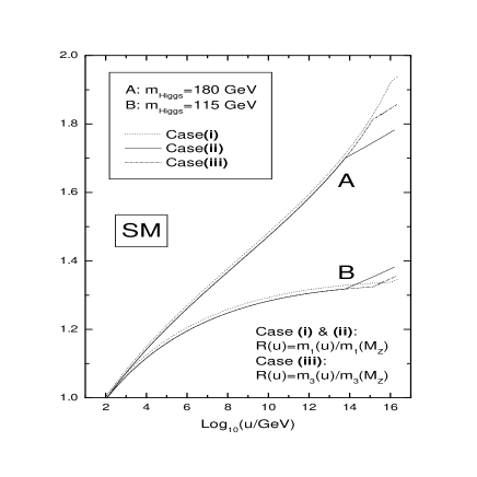
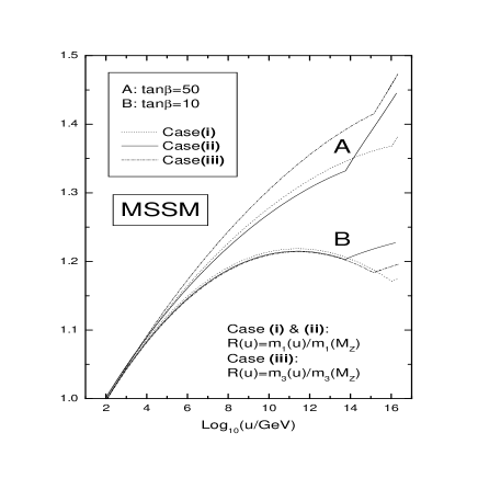
FIG. 1.: The RG evolution of a left-handed neutrino mass ($m_{1}$ of cases (i) and (ii), and $m_{3}$ of case (iii)) from $M_{\rm Z}$ to $\Lambda_{GUT}$, both in the SM and in the MSSM. At $M_{\rm Z}$, $\theta_{x}=33.2^{\circ}$, $\theta_{y}=45^{\circ}$, $\theta_{z}=5^{\circ}$, $\delta=45^{\circ}$ and $\rho=\sigma=5^{\circ}$. At $M_{3}$, $y_{\nu}=0.8$, $\theta_{1}=\theta_{2}=45^{\circ}$ and $\theta_{3}=\delta_{\nu}=\phi_{1}=\phi_{2}=5^{\circ}$.

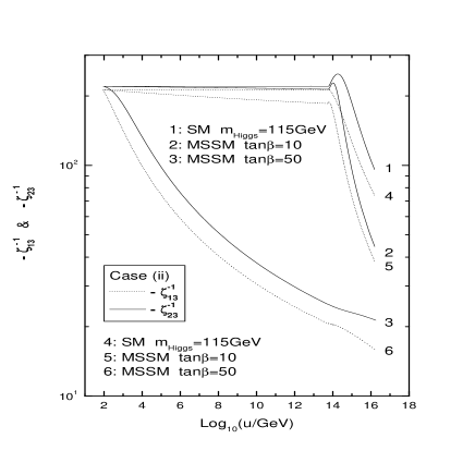
FIG. 2.: The typical evolution behavior of enhancing factors $\left(-\zeta_{ij}^{-1}\right)$ defined in Eq.(13), both in the SM and in the MSSM. At $M_{\rm Z}$, $\theta_{x}=33.2^{\circ}$, $\theta_{y}=45^{\circ},~{}\theta_{z}=5^{\circ},~{}\delta=45^{\circ}$ and $\rho=\sigma=5^{\circ}$. At $M_{3}$, $y_{\nu}=0.8$, $\theta_{1}=\theta_{2}=45^{\circ}$ and $\theta_{3}=\delta_{\nu}=\phi_{1}=\phi_{2}=5^{\circ}$.

FIG. 3.: Typical peaks of enhancing factors $\left(-\zeta_{ij}^{-1}\right)$ defined in Eq.(13) in nearly singular situations. At $M_{\rm Z}$, $\theta_{x}=33.2^{\circ}$, $\theta_{y}=45^{\circ}$, $\theta_{z}=5^{\circ}$, $\delta=55^{\circ}$ and $\rho=\sigma=5^{\circ}$. At $M_{3}$, $y_{\nu}=0.8$, $\theta_{1}=$ $\theta_{2}=89^{\circ}$ and $\theta_{3}=\delta_{\nu}=\phi_{1}=\phi_{2}=5^{\circ}$.

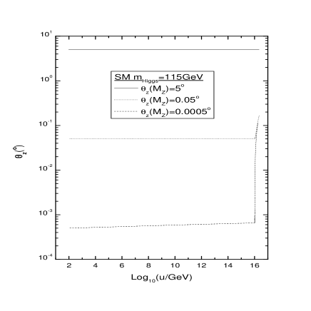
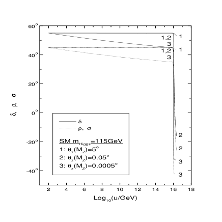
FIG. 4.: The typical evolution behavior of the mixing angle $\theta_{z}$ and CP-violating phases ($\delta,\rho,\sigma$) in the SM, in the normal hierarchy case. At $M_{\rm Z}$, $\theta_{x}=33.2^{\circ}$, $\theta_{y}=45^{\circ}$, $\delta=55^{\circ}$ and $\rho=\sigma=45^{\circ}$. At $M_{3}$, $y_{\nu}=0.8$, $\theta_{1}=\theta_{2}=\phi_{1}=\phi_{2}=45^{\circ}$ and $\theta_{3}=\delta_{\nu}=5^{\circ}$.

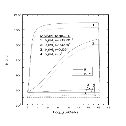
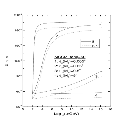
FIG. 5.: The typical evolution behavior of CP-violating phases ($\delta,\rho,\sigma$) in the MSSM, in the normal hierarchy case. At $M_{\rm Z}$, $\theta_{x}=33.2^{\circ}$, $\theta_{y}=45^{\circ}$, $\delta=55^{\circ}$ and $\rho=\sigma=45^{\circ}$. At $M_{3}$, $y_{\nu}=0.8$, $\theta_{1}=$ $\theta_{2}=\phi_{1}=\phi_{2}=45^{\circ}$ and $\theta_{3}=\delta_{\nu}=5^{\circ}$.

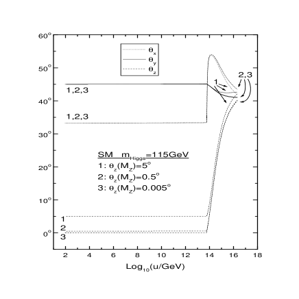
FIG. 6.: The typical evolution behavior of mixing angles ($\theta_{x},\theta_{y},\theta_{z}$) and CP-violating phases ($\delta,\rho,\sigma$) in the SM, in the near degeneracy case. At $M_{\rm Z}$, $\theta_{x}=33.2^{\circ}$, $\theta_{y}=45^{\circ}$, $\delta=55^{\circ}$, $\rho=80^{\circ}$ and $\sigma=5^{\circ}$. At $M_{3}$, $y_{\nu}=0.8$, $\theta_{1}=$ $\theta_{2}=45^{\circ}$ and $\phi_{1}=\phi_{2}=\theta_{3}=\delta_{\nu}=5^{\circ}$.

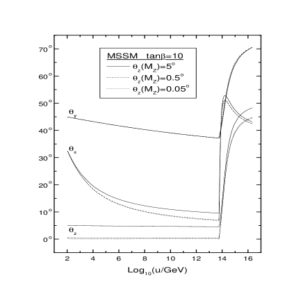
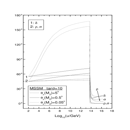
FIG. 7.: The typical evolution behavior of mixing angles ($\theta_{x},\theta_{y},\theta_{z}$) and CP-violating phases ($\delta,\rho,\sigma$) in the MSSM when $\tan\beta$ is small, in the near degeneracy case. At $M_{\rm Z}$, $\theta_{x}=33.2^{\circ}$, $\theta_{y}=45^{\circ}$, $\delta=55^{\circ}$ and $\rho=\sigma=45^{\circ}$. At $M_{3}$, $y_{\nu}=0.8$, $\theta_{1}=\theta_{2}=45^{\circ}$ and $\phi_{1}=\phi_{2}=\theta_{3}=\delta_{\nu}=5^{\circ}$.

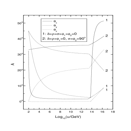
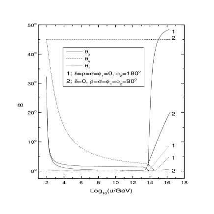
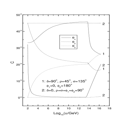
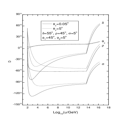
FIG. 8.: The typical evolution behavior of mixing angles ($\theta_{x},\theta_{y},\theta_{z}$) and CP-violating phases ($\delta,\rho,\sigma$) in the MSSM when $\tan\beta$ is large, in the near degeneracy case. Figures A, B and C illustrate cases in which the correction to a specific mixing angle is mostly enhanced or damped. Figure A is devoted to $\theta_{x}$, but we have also included the other two angles in the plot. Similarly, Figure B corresponds to $\theta_{y}$, and Figure C corresponds to $\theta_{z}$. Figure D serves to illustrate how $\theta_{z}$ may affect the RG evolution of CP-violating phases. At $M_{\rm Z}$, $\theta_{x}=33.2^{\circ}$, $\theta_{y}=45^{\circ}$ and $\theta_{z}=0.05^{\circ}$ (used in Figures A, B and C); at $M_{3}$, $y_{\nu}=0.8$, $\theta_{1}=$ $\theta_{2}=45^{\circ}$ and $\theta_{3}=\delta_{\nu}=5^{\circ}$. Initial values of CP-violating phases ($\delta$, $\rho$ and $\sigma$ at $M_{\rm Z}$, and $\phi_{1}$ and $\phi_{2}$ at $M_{3}$) are marked on the graphs.

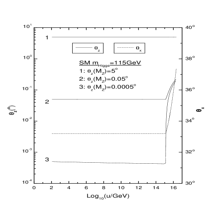
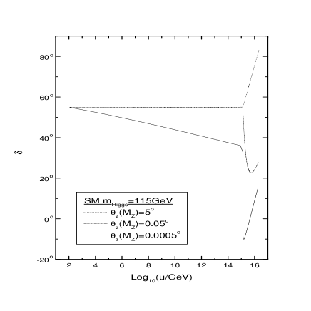
FIG. 9.: The typical evolution behavior of mixing angles $\theta_{x}$ and $\theta_{z}$ and CP-violating phases ($\delta,\rho,\sigma$) in the SM, in the inverted hierarchy case. At $M_{\rm Z}$, $\theta_{x}=33.2^{\circ}$, $\theta_{y}=45^{\circ}$, $\delta=55^{\circ}$, $\rho=85^{\circ}$ and $\sigma=5^{\circ}$; at $M_{3}$, $y_{\nu}=0.8$, $\theta_{1}=\theta_{2}=45^{\circ}$ and $\phi_{1}=\phi_{2}=\theta_{3}=\delta_{\nu}=5^{\circ}$.

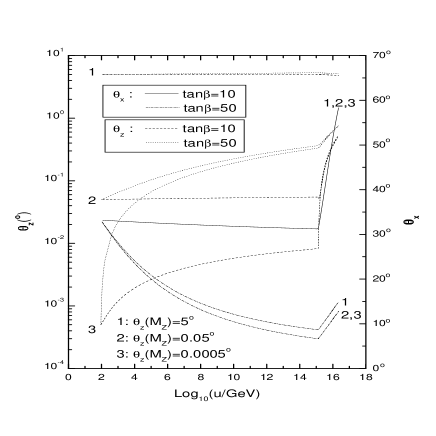
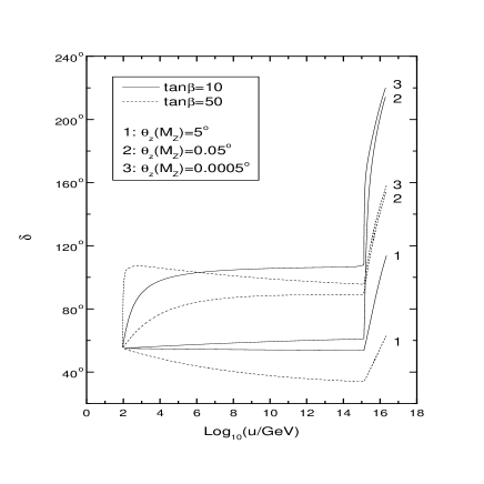
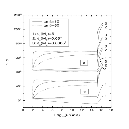
FIG. 10.: The typical evolution behavior of mixing angles $\theta_{x}$ and $\theta_{z}$ and CP-violating phases ($\delta,\rho,\sigma$) in the MSSM, in the inverted hierarchy case. At $M_{\rm Z}$, $\theta_{x}=33.2^{\circ}$, $\theta_{y}=45^{\circ}$ and $\delta=55^{\circ}$. Also at $M_{\rm Z}$, $\rho=\sigma=5^{\circ}$ in the plot of $\theta_{x}$, but $\rho=85^{\circ}$ and $\sigma=5^{\circ}$ in the plot of $\theta_{z},\delta,\rho$ and $\sigma$. At $M_{3}$, $y_{\nu}=0.8$, $\theta_{1}=\theta_{2}=45^{\circ}$ and $\phi_{1}=\phi_{2}=\theta_{3}=\delta_{\nu}=5^{\circ}$.