The two-photon exchange contribution to elastic electron-nucleon scattering at large momentum transfer

Abstract

We estimate the two-photon exchange contribution to elastic electron-proton scattering at large momentum transfer by using a quark-parton representation of virtual Compton scattering. We thus can relate the two-photon exchange amplitude to the generalized parton distributions which also enter in other wide angle scattering processes. We find that the interference of one- and two-photon exchange contribution is able to substantially resolve the difference between electric form factor measurements from Rosenbluth and polarization transfer experiments. Two-photon exchange has additional consequences which could be experimentally observed, including nonzero polarization effects and a positron-proton/electron-proton scattering asymmetry. The predicted Rosenbluth plot is no longer precisely linear; it acquires a measurable curvature, particularly at large laboratory angle.

I Introduction

There are two experimental methods for extracting the ratio of electric ($G_{E}^{p}$) to magnetic ($G_{M}^{p}$) proton form factors from electron-proton scattering: unpolarized measurements employing the Rosenbluth separation technique, and polarization experiments. In the latter case, one measures the correlation of the spin of the incident polarized electron with the polarization components of the outgoing proton, parallel $P_{l}$ or perpendicular $P_{s}$ (in the scattering plane) to its momentum Jones00 ; Gayou02 ; Arn81 . The ratio of cross sections for the two outgoing proton polarizations gives $G_{E}/G_{M}$ directly:

$${P_{s}\over P_{l}}=-\sqrt{2\varepsilon\over\tau(1+\varepsilon)}\ {G_{E}(Q^{2})\over G_{M}(Q^{2})}\ .$$ (1)

The kinematic functions $\varepsilon$ and $\tau$ are

$$\tau\equiv{Q^{2}\over 4M^{2}}\ ,$$ (2)

and

$${1\over\varepsilon}\equiv 1+2(1+\tau)\tan^{2}{\theta\over 2}\ ,$$ (3)

where $Q^{2}=-q^{2}=-t$ is the momentum transfer squared, $\theta$ is the laboratory scattering angle, and $0\leq\varepsilon\leq 1$. Equivalent information may be obtained in scattering of longitudinally polarized electrons on a polarized proton target.

The Rosenbluth method relies on measuring the differential cross section

$${d\sigma\over d\Omega_{Lab}}\propto G_{M}^{2}+\frac{\varepsilon}{\tau}G_{E}^{2}\ ,$$ (4)

with the proportionality factor being well known, and isolating the $\varepsilon$ dependent term. In each case, the extraction method for $G_{E}/G_{M}$ assumes single-photon exchange between the electron and nucleon.

Recent polarization experiments at the Thomas Jefferson Laboratory (JLab) Chr04 ; Arr03 have confirmed the earlier Rosenbluth measurements from SLAC  Slac94 . However, at large $Q^{2}$, all of the Rosenbluth measurements are at distinct variance with JLab measurements of $G^{p}_{E}/G^{p}_{M}$ obtained using the polarization technique Jones00 ; Gayou02 . Since $G_{E}^{p}$ contributes to the unpolarized cross section at only a few percent level for the $Q^{2}$ range in question, it is necessary to identify any possible systematic corrections to the Rosenbluth measurements at the percent level which could be responsible for this discrepancy.

One possible explanation for the discrepancy between the Rosenbluth and polarization methods is the presence of two-photon exchange effects, beyond those which have already been accounted for in the standard treatment of radiative corrections. A general study of two- (and multi)-photon exchange contributions to the elastic electron-proton scattering observables was given in GV03 . In that work, it was noted that the interference of the two-photon exchange amplitude with the one-photon exchange amplitude could be comparable in size to the $(G^{p}_{E})^{2}$ term in the unpolarized cross section at large $Q^{2}$. In contrast, the two-photon exchange effects do not impact the polarization-transfer extraction of $G_{E}/G_{M}$ in an equally significant way. Thus a missing and unfactorizable part of the two-photon exchange amplitude at the level of a few percent may well explain the discrepancy between the two methods.

Realistic calculations of elastic electron-nucleon scattering beyond the Born approximation are required in order to demonstrate in a quantitative way that two-photon exchange effects are indeed able to resolve this discrepancy. In particular, one wants to study quantitatively the “hard” corrections which will arise when both exchanged photons are far off shell or the intermediate nucleon state suffers inelastic excitations. Calculations of these corrections require a knowledge of the internal structure of the nucleon and thus could not be included in the classic oldyennie ; MoTsai68 and were not included in the more recent MT00 ; Andrei01 calculations of radiative corrections to $eN$ elastic scattering.

A first step was performed recently in BMT03 , where the contribution to the two-photon exchange amplitude was calculated for the elastic nucleon intermediate state. In that calculation it was found that the two-photon exchange correction with an intermediate nucleon has the proper sign and magnitude to partially resolve the discrepancy between the two experimental techniques.

In an earlier short note YCC04 , we reported the first calculation of the hard two-photon elastic electron-nucleon scattering amplitude at large momentum transfers by relating the required virtual Compton process on the nucleon to generalized parton distributions (GPD’s) which also enter in other wide angle scattering processes. This approach effectively sums all possible excitations of inelastic nucleon intermediate states. We found that the two-photon corrections to the Rosenbluth process indeed can substantially reconcile the two ways of measuring $G_{E}/G_{M}$. Our goal in this paper is to give a detailed account of our work, and to present numerical results for a number of quantities not included in the shorter report.

Perturbative QCD factorization methods for hard exclusive processes provide a systematic method for computing the scaling and angular dependence of real and virtual Compton scattering at large $t$. For example, PQCD predicts that the leading-twist amplitude for Compton scattering $\gamma p\to\gamma p$ can be factorized as a product of hard-scattering amplitudes $T_{H}(\gamma qqq\to\gamma qqq),$ where the quarks in each proton are collinear, convoluted with the initial and final proton distribution amplitudes $\phi(x_{i},Q)$ Brodsky:1981rp . All of the hard-scattering diagrams fall at the same rate at large momentum transfer whether or not the photons interact on the same line. Although, the predictions for the power-law falloff and angular dependence of Compton scattering are consistent with experiment, the leading-twist PQCD calculations of the wide angle Compton amplitudes appear to substantially underpredict the magnitude of the observed Compton cross sections Brooks:2000nb .

Since an exact QCD analysis of virtual Compton scattering does not appear practical, we have modeled the hard two-photon exchange amplitude using the “handbag approximation” Brodsky:1973hm , in which both photons interact with the same quark. The struck quark is treated as quasi-on shell. In particular, we have neglected the amplitudes where the two hard protons connect to different quarks, the “cat’s ears” diagrams, as well as the diagrams in which gluons interact on the fermion line between the two currents. The handbag diagrams contain the “$J=0$” fixed pole, the essential energy-independent contribution to the real part of Compton amplitude which arises due to the local structure of the quark current Damashek:1969xj ; Brodsky:1971zh . The handbag approximation has proven phenomenologically successful in describing wide-angle Compton scattering at moderate energies and momentum transfers. As we shall show, the handbag approximation allows the two-photon exchange amplitude to be linked to the generalized parton distributions (GPD’s) Die99 ; Rad98 ; Huang:2001ej , thus providing considerable phenomenological guidance.

Brooks and Dixon and Vanderhaeghen et al. Brooks:2000nb have shown that PQCD diagrams where the photons attach to the same quark dominate the Compton amplitude on the proton, except at backward center-of-mass angles.. The dominance of the handbag diagrams in the PQCD analysis provides some justification for the the use of the handbag approximation. However, it should be noted that Gunion and Blankenbecler Gunion:1970yy have shown that electron-deuteron scattering is dominated by the cat’s ears diagrams at large momentum transfer provided that the deuteron wave function has Gaussian fall-off. The dominance of the handbag diagrams thus depends on the nature of the QCD wave functions, and the precise situation in the present case remains a subject for future study.

Recently, a new category of Rosenbluth data has become available where the recoiling proton is detected Qattan:2004ht . The new data appear to confirm the older data, where the scattered electron was detected. The two-photon exchange contributions are the same whatever particle is detected. However, the bremsstrahlung corrections, which are added to obtain an infrared finite result, are different. We shall defer detailed discussion of the proton-detected data until we can reevaluate the original proton-observed electron-proton bremsstrahlung interference calculations oldyennie ; oldkrass as well as examine the radiative corrections which have been applied to the new data Ent:2001hm ; Qattan:2004ht .

The plan of this paper is as follows:

The next section is devoted to kinematics, including the definitions of the invariants which define the scattering amplitudes and the formulae for the cross sections and polarizations in terms of those invariants. There are choices in the definitions of the invariants. We have presented the bulk of the paper with one choice; a sometimes useful alternative choice is summarized with cross section and polarization formulas in Appendix A. Section III gives analytic results for the two-photon exchange scattering amplitudes at the electron-quark level, the hard scattering amplitudes required for the partonic calculation of two-photon exchange in electron-nucleon scattering. We have generally treated the quarks as massless. A quantitative discussion of modifications following from finite quark mass appears in Appendix B. Section IV details the embedding of the partonic amplitude within the nucleon scattering amplitude, using dominance of handbag amplitudes and GPD’s. This section also discusses the particular GPD’s which we have used in our numerical calculations. Section V shows numerical results, given graphically, for cross sections, single spin asymmetries, polarization transfers, and positron-proton vs. electron-proton comparisons. Section V also includes commentary about the possibility of extending the calculations to backward scattering (small values of $|u|$), and an assessment of how well two-photon physics reconciles the Rosenbluth and polarization transfer measurements of $G_{E}/G_{M}$. Section VI summarizes our conclusions.

II Elastic electron-nucleon scattering observables

In order to describe elastic electron-nucleon scattering,

$$l(k,h)+N(p,\lambda_{N})\rightarrow l(k^{\prime},h^{\prime})+N(p^{\prime},\lambda^{\prime}_{N}),$$ (5)

where $h$, $h^{\prime}$, $\lambda_{N}$, and $\lambda^{\prime}_{N}$ are helicities, we adopt the definitions

$$P=\frac{p+p^{\prime}}{2},\,K=\frac{k+k^{\prime}}{2},\,q=k-k^{\prime}=p^{\prime}-p\ ,$$ (6)

define the Mandelstam variables

$$s=(p+k)^{2},\quad t=q^{2}=-Q^{2},\quad u=(p-k^{\prime})^{2},$$ (7)

let $\nu\equiv K\cdot P$, and let $M$ be the nucleon mass.

The $T$-matrix helicity amplitudes are given by

$$T^{h^{\prime},h}_{\lambda^{\prime}_{N},\lambda_{N}}\equiv\left\langle k^{\prime},h^{\prime};p^{\prime},\lambda^{\prime}_{N}\right|T\left|k,h;p,\lambda_{N}\right\rangle\ .$$ (8)

Parity invariance reduces the number of independent helicity amplitudes from 16 to 8. Time reversal invariance further reduces the number to 6 Goldb57 . Further still, in a gauge theory lepton helicity is conserved to all orders in perturbation theory when the lepton mass is zero. We shall neglect the lepton mass. This finally reduces the number of independent helicity amplitudes to 3, which one may for example choose as

$$T^{+,+}_{+,+}\ ;\quad T^{+,+}_{-,-}\ ;\quad T^{+,+}_{-,+}=T^{+,+}_{+,-}\ .$$ (9)

(The phase in the last equality is for particle momenta in the $xz$ plane, and is valid whether we are in the center-of-mass frame, the Breit frame, or the symmetric frame to be defined below.)

Alternatively, one can expand in terms of a set of three independent Lorentz structures, multiplied by three generalized form factors. Only vector or axial vector lepton currents can appear in order to ensure lepton helicity conservation. A possible $T$-matrix expansion is (removing an overall energy-momentum conserving $\delta$-function),

$$T_{h,\,\lambda^{\prime}_{N}\lambda_{N}}={e^{2}\over Q^{2}} \Bigg{\{} \bar{u}(k^{\prime},h)\gamma_{\mu}u(k,h)\times\bar{u}(p^{\prime},\lambda^{\prime}_{N})\left[\gamma^{\mu}G^{\prime}_{M}-{P^{\mu}\over M}F^{\prime}_{2}\right]u(p,\lambda_{N})$$ (10)

$$+ \bar{u}(k^{\prime},h)\gamma_{\mu}\gamma_{5}u(k,h)\times\bar{u}(p,\lambda^{\prime}_{N})\,\gamma^{\mu}\gamma^{5}G^{\prime}_{A}\,u(p,\lambda_{N})\ \ \Bigg{\}}\ .$$

This expansion is general. The overall factors and the notations $G^{\prime}_{M}$ and $F^{\prime}_{2}$ have been chosen to have a straightforward connection to the standard form factors in the one-photon exchange limit.

There is no lowest order axial vector vertex in QED: the effective axial vertex in the expansion arises from multiple photon exchanges and vanishes in the one-photon exchange limit. One may eliminate the axial-like term using the identity

$$\bar{u}(k^{\prime})\gamma\cdot Pu(k)\times\bar{u}(p^{\prime})\gamma\cdot Ku(p) = {s-u\over 4}\,\bar{u}(k^{\prime})\gamma_{\mu}u(k)\times\bar{u}(p^{\prime})\gamma^{\mu}u(p)$$ (11)

$$+ {t\over 4}\,\bar{u}(k^{\prime})\gamma_{\mu}\gamma_{5}u(k)\times\bar{u}(p^{\prime})\gamma^{\mu}\gamma^{5}u(p)\ ,$$

which is valid for massless leptons and any nucleon mass. Hence, an equivalent $T$-matrix expansion is

$$T_{h,\,\lambda^{\prime}_{N}\lambda_{N}}\, = \,\frac{e^{2}}{Q^{2}}\,\bar{u}(k^{\prime},h)\gamma_{\mu}u(k,h)\,$$

$$\times \,\bar{u}(p^{\prime},\lambda^{\prime}_{N})\left(\tilde{G}_{M}\,\gamma^{\mu}-\tilde{F}_{2}\frac{P^{\mu}}{M}+\tilde{F}_{3}\frac{\gamma\cdot KP^{\mu}}{M^{2}}\right)u(p,\lambda_{N})\ .$$

Knowing both expansions of the scattering amplitude is useful, particularly when making comparison to other work. Our analysis will primarily use the second expansion, with the invariants denoted with tildes. A selection of expressions using the primed invariants is given in Appendix A.

The scalar quantities $\tilde{G}_{M}$, $\tilde{F}_{2}$, and $\tilde{F}_{3}$ are complex functions of two variables, say $\nu$ and $Q^{2}$. We will also use

$$\tilde{G}_{E}\equiv\tilde{G}_{M}-(1+\tau)\tilde{F}_{2}\ .$$ (13)

In order to easily identify the one- and two-photon exchange contributions, we introduce the notation $\tilde{G}_{M}=G_{M}+\delta\tilde{G}_{M}$, and $\tilde{G}_{E}=G_{E}+\delta\tilde{G}_{E}$, where $G_{M}$ and $G_{E}$ are the usual proton magnetic and electric form factors, which are functions of $Q^{2}$ only and are defined from matrix elements of the electromagnetic current. The amplitudes $\tilde{F}_{3}=\delta\tilde{F}_{3}$, $\delta\tilde{G}_{M}$, and $\delta\tilde{G}_{E}$, originate from processes involving the exchange of at least two photons, and are of order $e^{2}$ (relative to the factor $e^{2}$ in Eq. (II)).

The cross section without polarization is

$${d\sigma\over d\Omega_{Lab}}={\tau\sigma_{R}\over\epsilon(1+\tau)}{d\sigma_{NS}\over d\Omega_{Lab}}\ ,$$ (14)

where $\tau\equiv Q^{2}/(4M^{2})$, $\varepsilon$ is

$$\varepsilon=\left(1+2(1+\tau)\tan^{2}{\theta\over 2}\right)^{-1}={(s-u)^{2}+t(4M^{2}-t)\over(s-u)^{2}-t(4M^{2}-t)}\ ,$$ (15)

$\theta$ is the electron Lab scattering angle, the “no structure” cross section is

$${d\sigma_{NS}\over d\Omega_{Lab}}={4\alpha^{2}\cos^{2}{\theta\over 2}\over Q^{4}}\,{E^{\prime 3}\over E}\ ,$$ (16)

and $E$ and $E^{\prime}$ are the incoming and outgoing electron Lab energies. For one-photon exchange, $\varepsilon$ is the polarization parameter of the virtual photon. The reduced cross section including the two-photon exchange correction is given by GV03

$$\sigma_{R}=G_{M}^{2}+\frac{\varepsilon}{\tau}G_{E}^{2}\,+2\,G_{M}{\cal R}\left(\delta\tilde{G}_{M}+\varepsilon\frac{\nu}{M^{2}}\tilde{F}_{3}\right)+2\frac{\varepsilon}{\tau}G_{E}\,{\cal R}\left(\delta\tilde{G}_{E}+\frac{\nu}{M^{2}}\tilde{F}_{3}\right)+{\mathcal{O}}(e^{4}),$$ (17)

where ${\cal R}$ stands for the real part. Comparison to results elsewhere is often facilitated by the expression

$${\nu\over M^{2}}={s-u\over 4M^{2}}=\sqrt{\tau(1+\tau)\frac{1+\varepsilon}{1-\varepsilon}}\ .$$ (18)

The general expressions for the double polarization observables for an electron beam of positive helicity ($h=+1/2$) and for a recoil proton polarization along its momentum ($P_{l}$) or perpendicular, but in the scattering plane, to its momentum ($P_{s}$) can be derived as (for $m_{e}=0$) GV03 :

$$P_{s} = A_{s}=$$

$$= -\,\sqrt{\frac{2\varepsilon(1-\varepsilon)}{\tau}}\,\frac{1}{\sigma_{R}}\,\left\{G_{E}G_{M}+G_{E}\,{\cal R}\left(\delta\tilde{G}_{M}\right)+G_{M}\,{\cal R}\left(\delta\tilde{G}_{E}+\frac{\nu}{M^{2}}\tilde{F}_{3}\right)+{\mathcal{O}}(e^{4})\right\},$$

$$P_{l} = -A_{l}=\sqrt{1-\varepsilon^{2}}\,\frac{1}{\sigma_{R}}\,\left\{G_{M}^{2}+2\,G_{M}\,{\cal R}\left(\delta\tilde{G}_{M}+\frac{\varepsilon}{1+\varepsilon}\frac{\nu}{M^{2}}\tilde{F}_{3}\right)+{\mathcal{O}}(e^{4})\right\},$$

The polarizations are related to the analyzing powers $A_{s}$ or $A_{l}$ by time-reversal invariance, as indicated above. Note that $P_{l}$ is precisely unity in the backward direction, $\varepsilon=0$. This follows generally from lepton helicity conservation and angular momentum conservation.

An observable which is directly proportional to the two- (or multi-) photon exchange is a single-spin observable which is given by the elastic scattering of an unpolarized electron on a proton target polarized normal to the scattering plane (or the recoil polarization $P_{n}$ normal to the scattering plane, which is exactly the same assuming time-reversal invariance). The corresponding single-spin asymmetry, which we refer to as the target (or recoil) normal spin asymmetry ($A_{n}$), is related to the absorptive part of the elastic $eN$ scattering amplitude RKR71 . Since the one-photon exchange amplitude is purely real, the leading contribution to $A_{n}$ is of order $O(e^{2})$, and is due to an interference between one- and two-photon exchange amplitudes. The general expression for $A_{n}$ in terms of the invariants for electron-nucleon elastic scattering is given by (in the limit $m_{e}=0$),

$$P_{n} = A_{n}=$$

$$= \sqrt{\frac{2\,\varepsilon\,(1+\varepsilon)}{\tau}}\,\,\frac{1}{\sigma_{R}}\left\{-\,G_{M}\,{\cal I}\left(\delta\tilde{G}_{E}+\frac{\nu}{M^{2}}\tilde{F}_{3}\right)\,+\,G_{E}\,{\cal I}\left(\delta\tilde{G}_{M}+\left(\frac{2\varepsilon}{1+\varepsilon}\right)\frac{\nu}{M^{2}}\tilde{F}_{3}\right)\right\}\,,$$

where $\cal I$ denotes the imaginary part.

Another single-spin observable is the normal beam asymmetry, which is discussed elsewhere normal_beam and which is also zero in the one-photon exchange approximation. It is proportional to the electron mass, and the asymmetry is of ${\cal O}(10^{-6})$ for GeV electrons. It is possibly observable in low energy elastic muon-proton scattering. It was measured in experiments at MIT/Bates and MAMI BSSA-Exp at electron beam energies below 1 GeV. It is possibly also observable in low-energy elastic muon-proton scattering.

III The two-photon exchange contribution to elastic electron-quark scattering

In order to estimate the two-photon exchange contribution to $\tilde{G}_{M}$, $\tilde{F}_{2}$ and $\tilde{F}_{3}$ at large momentum transfers, we will consider a partonic calculation illustrated in Fig. 1. To begin, we calculate the subprocess on a quark, denoted by the scattering amplitude $H$ in Fig. 1. Subsequently, we shall embed the quarks in the proton as described through the nucleon’s generalized parton distributions (GPD’s).

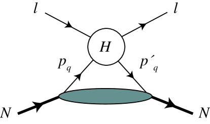
Figure 1: Handbag approximation for the elastic lepton-nucleon scattering at large momentum transfers. In the partonic scattering process (indicated by $H$), the lepton scatters from quarks in the nucleon, with momenta $p_{q}$ and $p^{\prime}_{q}$. The lower blob represents the GPD’s of the nucleon.

Elastic lepton-quark scattering,

$$l(k)+q(p_{q})\rightarrow l(k^{\prime})+q(p^{\prime}_{q})\ ,$$ (21)

is described by two independent kinematical invariants, $\hat{s}\equiv(k+p_{q})^{2}$ and $Q^{2}=-t=-(k-k^{\prime})^{2}$. We also introduce the crossing variable $\hat{u}\equiv(k-p^{\prime}_{q})^{2}$, which satisfies $\hat{s}+\hat{u}=Q^{2}$. The $T$-matrix for the two-photon part of the electron-quark scattering can be written as

$$H_{h,\,\lambda}\, = \,\frac{(e\,e_{q})^{2}}{Q^{2}}\,\bar{u}(k^{\prime},h)\gamma_{\mu}u(k,h)\,\cdot\,\bar{u}(p^{\prime}_{q},\lambda)\left(\,\tilde{f}_{1}\,\gamma^{\mu}\,+\,\tilde{f}_{3}\,\gamma.K\,P_{q}^{\mu}\,\right)u(p_{q},\lambda),$$ (22)

with $P_{q}\equiv(p_{q}+p^{\prime}_{q})/2$, where $e_{q}$ is the fractional quark charge (for a flavor $q$), and where $u(p_{q},\lambda)$ and $u(p^{\prime}_{q},\lambda)$ are the quark spinors with quark helicity $\lambda=\pm 1/2$, which is conserved in the scattering process for massless quarks. Quark helicity conservation leads to the absence of any analog of $\tilde{F}_{2}$ in the general expansion of Eq. (II).

In order to calculate the partonic scattering helicity amplitudes $H_{h,\lambda}$ of Eq. (22) at order $O(e^{4})$, we consider the two-photon exchange direct and crossed box diagrams of Fig. 2.

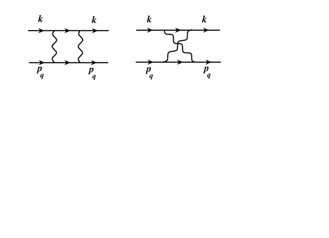
Figure 2: Direct and crossed box diagrams to describe the two-photon exchange contribution to the lepton-quark scattering process, corresponding with the blob denoted by $H$ in Fig. 1.

The two-photon exchange contribution to the elastic electron-scattering off spin 1/2 Dirac particles was first calculated in Ref. Nie71 , which we verified explicitly. For further use, we separate the amplitude $\tilde{f}_{1}$ for the scattering of massless electrons off massless quarks into a soft and hard part, i.e. $\tilde{f}_{1}=\tilde{f}_{1}^{soft}+\tilde{f}_{1}^{hard}$. The soft part corresponds with the situation where one of the photons in Fig. 2 carries zero four-momentum, and is obtained by replacing the other photon’s four-momentum by $q$ in both numerator and denominator of the loop integral grammer . This yields,

$${\cal R}\left(\tilde{f}_{1}^{soft}\right) = \frac{e^{2}}{4\pi^{2}}\,\left\{\ln\left(\frac{\lambda^{2}}{\sqrt{-\hat{s}\hat{u}}}\right)\ln\left|\frac{\hat{s}}{\hat{u}}\right|+\frac{\pi^{2}}{2}\right\},$$ (23)

$${\cal R}\left(\tilde{f}_{1}^{hard}\right) = \frac{e^{2}}{4\pi^{2}}\left\{\,\frac{1}{2}\,\ln\left|\frac{\hat{s}}{\hat{u}}\right|+\frac{Q^{2}}{4}\left[\frac{1}{\hat{u}}\ln^{2}\left|\frac{\hat{s}}{Q^{2}}\right|-\frac{1}{\hat{s}}\ln^{2}\left|\frac{\hat{u}}{Q^{2}}\right|-\frac{1}{\hat{s}}\pi^{2}\right]\right\},$$ (24)

where $\tilde{f}_{1}^{soft}$, which contains a term proportional to $\ln\lambda^{2}$ ($\lambda$ is an infinitesimal photon mass), is IR divergent. The amplitude $\tilde{f}_{3}$ resulting from the diagrams of Fig. 2 is IR finite, and its real part is

$${\cal R}\left(\tilde{f}_{3}\right)=\frac{e^{2}}{4\pi^{2}}\,\frac{1}{\hat{s}\,\hat{u}}\,\left\{\hat{s}\,\ln\left|\frac{\hat{s}}{Q^{2}}\right|+\hat{u}\,\ln\left|\frac{\hat{u}}{Q^{2}}\right|+\frac{\hat{s}-\hat{u}}{2}\left[\frac{\hat{s}}{\hat{u}}\ln^{2}\left|\frac{\hat{s}}{Q^{2}}\right|-\frac{\hat{u}}{\hat{s}}\ln^{2}\left|\frac{\hat{u}}{Q^{2}}\right|-\frac{\hat{u}}{\hat{s}}\pi^{2}\right]\right\}.$$ (25)

The correction to the electron-quark elastic cross section can be obtained from Eq. (17),

$$d\sigma\, = \,d\sigma_{1\gamma}\,\left[1+2\,{\cal R}\left(\tilde{f}_{1}\right)_{2\gamma}+\varepsilon\,\frac{\hat{s}-\hat{u}}{4}\,2\,{\cal R}\left(\tilde{f}_{3}\right)_{2\gamma}\right],$$ (26)

$$\equiv d\sigma_{1\gamma}\,\left(1+\delta_{2\gamma}\right),$$

where $d\sigma_{1\gamma}$ is the cross section in the one-photon exchange approximation and $\varepsilon=-2\,\hat{s}\,\hat{u}\,/\,(\hat{s}^{2}+\hat{u}^{2})$ in the massless limit. Using Eqs. (23, 24, 25), we obtain (for $e_{q}=+1$)

$$\delta_{2\gamma} = \frac{e^{2}}{4\pi^{2}}\,\left\{2\ln\left(\frac{\lambda^{2}}{Q^{2}}\right)\,\ln\left|\frac{\hat{s}}{\hat{u}}\right|\,\right.$$

$$+ \left.\frac{(\hat{s}-\hat{u})Q^{2}}{2\,(\hat{s}^{2}+\hat{u}^{2})}\left[\ln^{2}\left|\frac{\hat{s}}{Q^{2}}\right|+\ln^{2}\left|\frac{\hat{u}}{Q^{2}}\right|+\pi^{2}\right]+\frac{Q^{4}}{\hat{s}^{2}+\hat{u}^{2}}\,\left[\frac{\hat{u}}{Q^{2}}\ln\left|\frac{\hat{s}}{Q^{2}}\right|-\frac{\hat{s}}{Q^{2}}\ln\left|\frac{\hat{u}}{Q^{2}}\right|\right]\,\right\},$$

which is in agreement with the corresponding expression for electron-muon scattering obtained in Ref. Byt03 . The expressions of $\tilde{f}_{1}$ and $\tilde{f}_{3}$ can also be obtained through crossing from the corresponding expressions of the box diagrams for the process $e^{+}e^{-}\to\mu^{+}\mu^{-}$ as calculated in Ref. Khr73 .

We will need the expressions for the imaginary parts of $\tilde{f}_{1}$ and $\tilde{f}_{3}$ in order to calculate the normal spin asymmetry $A_{n}$. These imaginary parts originate solely from the direct two-photon exchange box diagram of Fig. 2 and are given by

$${\cal I}\left(\tilde{f}_{1}^{soft}\right) = -\frac{e^{2}}{4\pi}\,\ln\left(\frac{\lambda^{2}}{\hat{s}}\right),$$ (28)

$${\cal I}\left(\tilde{f}_{1}^{hard}\right) = -\frac{e^{2}}{4\pi}\left\{\frac{Q^{2}}{2\,\hat{u}}\ln\left(\frac{\hat{s}}{Q^{2}}\right)+\frac{1}{2}\right\},$$ (29)

$${\cal I}\left(\tilde{f}_{3}\right) = -\frac{e^{2}}{4\pi}\,\frac{1}{\hat{u}}\,\left\{\frac{\hat{s}-\hat{u}}{\hat{u}}\ln\left(\frac{\hat{s}}{Q^{2}}\right)+1\right\}.$$ (30)

Notice that the IR divergent part in Eq. (28) does not contribute when calculating the normal spin asymmetry $A_{n}$ of Eq. (II). Indeed at the quark level, one may complete the calculation for quark mass $m_{q}$ nonzero and find that $A_{n}$ is given by,

$$A_{n}=\frac{e_{q}e^{2}}{4\pi}\frac{m_{q}}{2\,Q}\,\frac{\sqrt{2\varepsilon(1+\varepsilon)}}{1+4\varepsilon m_{q}^{2}/Q^{2}}\,\frac{Q^{2}(Q^{2}+4m_{q}^{2})}{\hat{s}(\hat{s}-\hat{u})}\,\,$$ (31)

an IR finite quantity (cf. Barut60 ).

IV The handbag calculation of the two-photon exchange contribution to elastic electron-nucleon scattering

Having calculated the partonic subprocess, we next discuss how to embed the quarks in the nucleon. We begin by discussing the soft contributions. The handbag diagrams discussed so far have both photons coupled to the same quark. There are also contributions from processes where the photons interact with different quarks. One can show that the IR contributions from these processes, which are proportional to the products of the charges of the interacting quarks, added to the soft contributions from the handbag diagrams give the same result as the soft contributions calculated with just a nucleon intermediate state Brodsky:1968ea . Thus the low energy theorem for Compton scattering is satisfied. As discussed in the introduction, the hard parts which appear when the photons couple to different quarks, the so-called cat’s ears diagrams, are neglected in the handbag approximation.

For the real parts, the IR divergence arising from the direct and crossed box diagrams, at the nucleon level, is cancelled when adding the bremsstrahlung contribution from the interference of diagrams where a soft photon is emitted from the electron and from the proton. This provides a radiative correction term from the soft part of the boxes plus electron-proton bremsstrahlung which added to the lowest order term may be written as

$$\sigma_{soft}=\sigma_{1\gamma}\,\left(1+\delta_{2\gamma,\,soft}+\delta_{brems}^{ep}\right),$$ (32)

where $\sigma_{1\gamma}$ is the one-photon exchange cross section. In Eq. (32), the soft-photon contribution due to the nucleon box diagram is given by

$$\delta_{2\gamma,\,soft}=\frac{e^{2}}{2\pi^{2}}\left\{\ln\left(\frac{\lambda^{2}}{\sqrt{(s-M^{2})|u-M^{2}|}}\right)\,\ln\left|\frac{s-M^{2}}{u-M^{2}}\right|\right.$$ (33)

$$-\left.L\left(\frac{s-M^{2}}{s}\right)-\frac{1}{2}\ln^{2}\left(\frac{s-M^{2}}{s}\right)+{\cal R}\left[L\left(\frac{u-M^{2}}{u}\right)\right]+\frac{1}{2}\ln^{2}\left(\frac{u-M^{2}}{u}\right)+\frac{\pi^{2}}{2}\right\},$$

where $L$ is the Spence function defined by

$$L(z)=-\int_{0}^{z}\,dt\,\frac{\ln(1-t)}{t}\ .$$ (34)

The bremsstrahlung contribution where a soft photon is emitted from an electron and proton line (i.e., by cutting one of the (soft) photon lines in Fig. 2) was calculated in Ref. MT00 , which we verified explicitly, and is for the case that the outgoing electron is detected,

$$\delta_{brems}^{ep} = \frac{e^{2}}{2\pi^{2}}\bigg{\{}\ln\left(\frac{4\,(\Delta E)^{2}\,(s-M^{2})^{2}}{\lambda^{2}\,y\,(u-M^{2})^{2}}\right)\,\ln\left(\frac{s-M^{2}}{M^{2}-u}\right)$$ (35)

$$\qquad+\ L\left(1-\frac{1}{y}\,\frac{s-M^{2}}{M^{2}-u}\right)-L\left(1-\frac{1}{y}\,\frac{M^{2}-u}{s-M^{2}}\right)\bigg{\}},$$

where $\Delta E\equiv E_{e}^{\,{}^{\prime}el}-E_{e}^{\,{}^{\prime}}$ is the difference of the measured outgoing electron lab energy ($E_{e}^{\,{}^{\prime}}$) from its elastic value ($E_{e}^{\,{}^{\prime}el}$), and $y\equiv(\sqrt{\tau}+\sqrt{1+\tau})^{2}$. One indeed verifies that the sum of Eqs. (33,35) is IR finite. When comparing with elastic $ep$ cross section data, which are usually radiatively corrected using the procedure of Mo and Tsai, Ref. MoTsai68 , we have to consider only the difference of our $\delta_{2\gamma,\,soft}+\delta_{brems}^{ep}$ relative to the ${\cal O}(Z^{2})$ part, in their notation, of the radiative correction in MoTsai68 . Except for the $\pi^{2}/2$ term in Eq. (33), this difference was found to be below $10^{-3}$ for all kinematics considered in Fig. 3.

Having discussed the two-photon exchange contribution on the nucleon when one of the two photons is soft, we next discuss the contribution which arises from the hard part (that is, neither photons soft) of the partonic amplitude coming from the box diagrams. This part of the amplitude is calculated, in the kinematical regime where $s$, $-u$, and $Q^{2}$ are large compared to a hadronic scale ($s,-u,Q^{2}>>M^{2}$), as a convolution between a hard scattering electron-quark amplitude and a soft matrix element on the nucleon. It is convenient to choose a frame where $q^{+}=0$, as in DY70 , where we introduce light-cone variables $a^{\pm}\propto(a^{0}\pm a^{3})$ and choose the $z$-axis along the direction of $P^{3}$ (so that $P$ has a large + component). We use the symmetric frame, as in Die99 , where the external momenta and $q$ are

$$k = \left[\eta P^{+},\frac{1}{P^{+}}{Q^{2}\over 4\eta},\frac{1}{2}\vec{q}_{\perp}\right]\,,$$

$$k^{\prime} = \left[\eta P^{+},\frac{1}{P^{+}}{Q^{2}\over 4\eta},-\frac{1}{2}\vec{q}_{\perp}\right]\,,$$

$$q = \left[0,0,\vec{q}_{\perp}\right]\,,$$

$$p = \left[P^{+},\frac{1}{P^{+}}\left(M^{2}+\frac{Q^{2}}{4}\right),-\frac{1}{2}\vec{q}_{\perp}\right]\,,$$

$$p^{\prime} = \left[P^{+},\frac{1}{P^{+}}\left(M^{2}+\frac{Q^{2}}{4}\right),\frac{1}{2}\vec{q}_{\perp}\right]\,.$$ (36)

Then,

$$s=\frac{(1+\eta)^{2}}{4\eta}\,Q^{2}+(1+\eta)M^{2}\,,\qquad u=-\frac{(1-\eta)^{2}}{4\eta}\,Q^{2}+(1-\eta)M^{2}\,,$$ (37)

one may check that $s+u=2M^{2}+Q^{2}$ and also solve for the lepton light-front momentum fractions, $\eta=k^{+}/P^{+}=k^{\prime\,+}/P^{+}$, as

$$\eta=\frac{1}{Q^{2}+4\,M^{2}}\left[s-u-2\,\sqrt{M^{4}-s\,u}\,\right].$$ (38)

For comparison, forward scattering in the CM, $\theta_{\rm CM}=0^{\circ}$, matches to $\eta=0$ and backward scattering, $\theta_{\rm CM}=180^{\circ}$, matches to $\eta=(s-M^{2})/s$.

In the $q^{+}=0$ frame, the parton light-front momentum fractions are defined as $x=p_{q}^{+}/P^{+}=p_{q}^{\prime\,+}/P^{+}$. The active partons, on which the hard scattering takes place, are approximately on-shell. In the symmetric frame, we take the spectator partons to have transverse momenta that are small (relative to $P$) and can be neglected when evaluating the hard scattering amplitude $H$ in Fig. 1. The Mandelstam variables for the process (21) on the quark, which enter in the evaluation of the hard scattering amplitude, are then given by

$$\hat{s}=\frac{(x+\eta)^{2}}{4\,x\,\eta}\,Q^{2}\,,\hskip 28.45274pt\hat{u}=-\frac{(x-\eta)^{2}}{4\,x\,\eta}\,Q^{2}.$$ (39)

Note that in the limit $x\simeq 1$, where $\hat{s}\simeq s$ and $\hat{u}\simeq u$ , the quark momenta are collinear with their parent hadron momenta, i.e. $p_{q}\simeq p$ and $p^{\prime}_{q}\simeq p^{\prime}$. This is the simplest situation for the handbag approximation, in which it was shown possible to factorize the wide angle real Compton scattering amplitude in terms of a hard scattering process and a soft overlap of hadronic light-cone wave functions, which in turn can be expressed as moments of generalized parton distributions (GPD’s) Rad98 ; Die99 . In the following we will extend the handbag Die99 ; brodsky71 formalism to calculate the two-photon exchange amplitude to elastic electron-nucleon scattering at moderately large momentum transfers, and derive the amplitude within a more general unfactorized framework by keeping the $x$ dependence in the hard scattering amplitude (i.e., by not taking the $x\to 1$ limit from the outset).

For the process (5) in the kinematical regime $s,-u,Q^{2}>>M^{2}$, the (unfactorized) handbag approximation implies that the $T$-matrix can be written as

$$T_{h,\,\lambda^{\prime}_{N}\lambda_{N}}^{hard}=\int_{-1}^{1}\frac{dx}{x}\,\sum_{q}\frac{1}{2}\left[H_{h,\,+\frac{1}{2}}^{hard}+H_{h,\,-\frac{1}{2}}^{hard}\right]\times$$ (40)

$$\qquad\times\frac{1}{2}\left[H^{q}\left(x,0,q^{2}\right)\,\bar{u}(p^{\prime},\lambda^{\prime}_{N})\,\gamma\cdot n\,u(p,\lambda_{N})+E^{q}\left(x,0,q^{2}\right)\,\bar{u}(p^{\prime},\lambda^{\prime}_{N})\,\frac{i\,\sigma^{\mu\nu}\,n_{\mu}q_{\nu}}{2M}\,u(p,\lambda_{N})\right]$$

$$\qquad+\int_{-1}^{1}\frac{dx}{x}\,\sum_{q}\frac{1}{2}\left[H_{h,\,+\frac{1}{2}}^{hard}-H_{h,\,-\frac{1}{2}}^{hard}\right]\cdot\frac{1}{2}\mathrm{sgm}(x)\,\tilde{H}^{q}\left(x,0,q^{2}\right)\bar{u}(p^{\prime},\lambda^{\prime}_{N})\,\gamma\cdot n\,\gamma_{5}\,u(p,\lambda_{N}),$$

where the hard scattering amplitude $H^{hard}$ is evaluated using the hard part of $\tilde{f}_{1}$ and $\tilde{f}_{3}$, with kinematics $\hat{s}$ and $\hat{u}$ according to Eq. (39), and where $n^{\mu}$ is a Sudakov four-vector ($n^{2}=0$), which can be expressed as

$$n^{\mu}\,=\,\frac{2}{\sqrt{M^{4}-su}}\,\left\{-\eta\,P^{\mu}\,+\,K^{\mu}\right\}.$$ (41)

Furthermore in Eq. (40), $H^{q},E^{q},\tilde{H}^{q}$ are the GPD’s for a quark $q$ in the nucleon (for a review see, e.g., Ref. GPV01 ).

¿From Eqs. (II), (22), and (40) the hard $2\gamma$ exchange contributions to $\delta\tilde{G}_{M}$, $\delta\tilde{G}_{E}$, and $\tilde{F}_{3}$ are obtained (after some algebra) as

$$\delta\tilde{G}_{M}^{hard} = C,$$ (42)

$$\delta\tilde{G}_{E}^{hard} = -\left(\frac{1+\varepsilon}{2\varepsilon}\right)\,(A-C)+\sqrt{\frac{1+\varepsilon}{2\varepsilon}}\,B,$$ (43)

$$\tilde{F}_{3} = \frac{M^{2}}{\nu}\left(\frac{1+\varepsilon}{2\varepsilon}\right)\,(A-C),$$ (44)

with

$$A \equiv \int_{-1}^{1}\frac{dx}{x}\frac{\left[(\hat{s}-\hat{u})\tilde{f}_{1}^{hard}-\hat{s}\hat{u}\tilde{f}_{3}\right]}{(s-u)}\sum_{q}e_{q}^{2}\,\left(H^{q}+E^{q}\right),$$

$$B \equiv \int_{-1}^{1}\frac{dx}{x}\frac{\left[(\hat{s}-\hat{u})\tilde{f}_{1}^{hard}-\hat{s}\hat{u}\tilde{f}_{3}\right]}{(s-u)}\sum_{q}e_{q}^{2}\,\left(H^{q}-\tau E^{q}\right),$$

$$C \equiv \int_{-1}^{1}\frac{dx}{x}\,\tilde{f}_{1}^{hard}\,\mathrm{sgm}(x)\,\sum_{q}e_{q}^{2}\,\tilde{H}^{q},$$ (45)

where note that in Eqs. (42)-(44), the partonic amplitude $\tilde{f}_{1}$ has its soft IR divergent part removed as discussed before.

Equations (42)-(44) reduce to the partonic amplitudes in the limit $M\to 0$ by considering a quark target for which the GPD’s are given by,

$$H^{q} \to \delta(1-x)\,,$$

$$E^{q} \to 0\,,$$

$$\tilde{H}^{q} \to \delta(1-x)\,.$$ (46)

In this limit, and using the identity

$$-\frac{\hat{s}\hat{u}}{\hat{s}-\hat{u}}=\frac{\hat{s}-\hat{u}}{4}\frac{2\varepsilon}{1+\varepsilon}\,,$$ (47)

we find that

$$\delta\tilde{G}_{M}^{hard} \to \sum_{q}e^{2}_{q}\tilde{f}_{1}^{hard}\,,$$

$$\frac{\delta\tilde{F}_{2}}{M} \to 0\,,$$

$$\frac{\delta\tilde{F}_{3}}{M^{2}} \to \sum_{q}e_{q}^{2}\tilde{f}_{3}\,.$$ (48)

¿From the integrals $A$, $B$, and $C$, and the usual form factors, we can directly construct the observables. The cross section is

$$\sigma_{R}=\sigma_{R,soft}+\sigma_{R,hard}\,,$$ (49)

where

$$\sigma_{R,hard}=(1+\varepsilon)\,G_{M}\,{\cal R}\left(A\right)+\sqrt{2\,\varepsilon\,(1+\varepsilon)}\frac{1}{\tau}\,G_{E}\,{\cal R}\left(B\right)+(1-\varepsilon)\,G_{M}\,{\cal R}\left(C\right)\,.$$ (50)

¿From Eqs. (32) to (35) and the discussion surrounding them, we learned that to a good approximation the result for the soft part can be written as

$$\sigma_{R,soft}=\sigma_{R,1\gamma}\left(1+\pi\alpha+\delta^{MT}\right)\,,$$ (51)

where $\delta^{MT}$ is the correction given in Ref. MoTsai68 . Since the data is very commonly corrected using MoTsai68 , let us define $\sigma_{R}^{\ MT\ corr}\equiv\sigma_{R}/(1+\delta^{MT})$. Then an accurate relationship between the data with Mo-Tsai corrections already included and the form factors is

$$\sigma_{R}^{\ MT\ corr}=\left(G_{M}^{2}+\frac{\varepsilon}{\tau}G_{E}^{2}\right)(1+\pi\alpha)+\sigma_{R,hard}\,,$$ (52)

where the extra terms on the right-hand-side come from two-photon exchange and ${\cal O}(e^{4})$ terms are not included. The reader may marginally improve the expression by including with the $(1+\pi\alpha)$ factor the circa 0.1% difference between our actual soft results and those of MoTsai68 ; from our side the relevant formulas are the aforementioned (32) to (35). Since the Mo-Tsai corrections are so commonly made in experimental papers before reporting the data, the “$MT\ corr$” superscript will be understood rather than explicit when we show cross section plots below. Finally, before discussing polarization, the fact that a $\pi^{2}/2$ term, or $(\pi\alpha)$ term after multiplying in the overall factors, sits in the soft corrections has to do with the specific criterion we used, that of Ref. grammer , to separate the soft from hard parts. The term cannot be eliminated; with a different criterion, however, that term can move into the hard part.

The double polarization observables of Eqs. (53,54) are given by

$$P_{s} = -\,\sqrt{\frac{2\varepsilon(1-\varepsilon)}{\tau}}\,\frac{1}{\sigma_{R}}\,\left\{G_{E}G_{M}+G_{E}\,{\cal R}\left(C\right)+G_{M}\,\sqrt{\frac{1+\varepsilon}{2\,\varepsilon}}\,{\cal R}\left(B\right)+{\mathcal{O}}(e^{4})\right\},$$ (53)

$$P_{l} = \sqrt{1-\varepsilon^{2}}\,\frac{1}{\sigma_{R}}\,\left\{G_{M}^{2}+\,G_{M}\,{\cal R}\left(A+C\right)+{\mathcal{O}}(e^{4})\right\},$$ (54)

and the target normal spin asymmetry of Eq. (II) is

$$A_{n} = \sqrt{\frac{2\,\varepsilon\,(1+\varepsilon)}{\tau}}\,\frac{1}{\sigma_{R}}\left\{G_{E}\,{\cal I}\left(A\right)-\sqrt{\frac{1+\varepsilon}{2\varepsilon}}\,G_{M}\,{\cal I}\left(B\right)\right\},$$ (55)

One sees from Eq. (55) that $A_{n}$ does not depend on the GPD $\tilde{H}$.

We will need to specify a model for the GPD’s in order to estimate the crucial integrals Eqs. (45) for the two-photon exchange amplitudes We will present results from two different GPD models: a gaussian model and a modified Regge model.

First, following Ref. Rad98 , we use a gaussian valence model which is unfactorized in $x$ and $Q^{2}$ for the GPD’s $H$ and $\tilde{H}$,

$$H^{q}(x,0,q^{2})\,=\,q_{v}(x)\;\exp\left(-\frac{(1-x)\,Q^{2}}{4\,x\,\sigma}\right),$$ (56)

$$\tilde{H}^{q}(x,0,q^{2})\,=\,\Delta q_{v}(x)\;\exp\left(-\frac{(1-x)\,Q^{2}}{4\,x\,\sigma}\right),$$ (57)

where $q_{v}(x)$ is the valence quark distribution and $\Delta q_{v}(x)$ the polarized valence quark distribution. In the following estimates we take the unpolarized parton distributions at input scale $Q_{0}^{2}$ = 1 GeV² from the MRST2002 global NNLO fit mrst02 as

$$u_{v} = 0.262\,x^{-0.69}(1-x)^{3.50}\left(1+3.83\,x^{0.5}+37.65\,x\right),$$

$$d_{v} = 0.061\,x^{-0.65}(1-x)^{4.03}\left(1+49.05\,x^{0.5}+8.65\,x\right).$$

For the polarized parton distributions, we adopt the recent NLO analysis of Ref. Lea02 , which at input scale $Q_{0}^{2}$ = 1 GeV² yields

$$\Delta u_{v} = 0.505x^{-0.33}(1-x)^{3.428}\left(1+2.179x^{0.5}+14.57x\right),$$

$$\Delta d_{v} = -0.0185x^{-0.73}(1-x)^{3.864}\left(1+35.47x^{0.5}+28.97x\right).$$

For the GPD $E$, whose forward limit is unknown, we adopt a valence parametrization multiplied with $(1-x)^{2}$ to be consistent with the $x\to 1$ limit Yuan03 . This gives

$$E^{q}(x,0,q^{2})=\frac{\kappa^{q}}{N^{q}}(1-x)^{2}q_{v}(x)\exp\left(-\frac{(1-x)Q^{2}}{4\,x\,\sigma}\right),$$ (58)

where the normalization factors $N^{u}=1.377$ and $N^{d}=0.7554$ are chosen in such a way that the first moments of $E^{u}$ and $E^{d}$ at $Q^{2}=0$ yield the anomalous magnetic moments $\kappa^{u}=2\kappa^{p}+\kappa^{n}=1.673$ and $\kappa^{d}=\kappa^{p}+2\kappa^{n}=-2.033$ respectively. Furthermore, the parameter $\sigma$ in Eqs. (56,57,58) is related to the average transverse momentum of the quarks inside the nucleon by $\sigma=5\,<k_{\perp}^{2}>$. Its value has been estimated in Ref. Die99 as $\sigma\simeq 0.8$ GeV², which we will adopt in the following calculations.

The GPD’s just described were used in our shorter note YCC04 . Recently, GPD’s whose first moments give a better account of the nucleon form factors have become available guidal . These GPD’s we refer to as a modified Regge model guidal , and entail

$$H^{q}(x,0,q^{2}) = q_{v}(x)\;x^{a^{\prime}_{1}(1-x)Q^{2}}\ ,$$

$$E^{q}(x,0,q^{2}) = \frac{\kappa^{q}}{N^{q}}(1-x)^{\eta_{q}}q_{v}(x)\;x^{a^{\prime}_{2}(1-x)Q^{2}}\ ,$$

$$\tilde{H}^{q}(x,0,q^{2}) = \Delta q_{v}(x)\;x^{\tilde{a}^{\prime}_{1}(1-x)Q^{2}}\ .$$ (59)

We still use the same $q_{v}$ and the same $\Delta q_{v}$ as given above. The five parameters are

$$\alpha^{\prime}_{1} = 1.098{\rm\ GeV}^{-2},\qquad\alpha^{\prime}_{2}=1.158{\rm\ GeV}^{-2},\qquad\tilde{\alpha}^{\prime}_{1}=1.000{\rm\ GeV}^{-2},$$

$$\eta_{u} = 1.52,\qquad\eta_{d}=0.31,$$ (60)

and the normalization factors here become $N_{u}=1.519$ and $N_{d}=0.9447$. The modified Regge GPD’s formally do not give convergence at low $Q^{2}$ for integrands with negative powers of $x$, such as we have here (or as one finds in Die99 ). The integrals could be defined by analytically continuing in the Regge intercept Damashek:1969xj ; Brodsky:1971zh . We will use them only for $Q^{2}\geq 2$ GeV², and all the integrals converge straightforwardly.

We shall investigate in forthcoming plots the sensitivity of the results to the two GPD’s.

V Results

V.1 Cross section

In Fig. 3, we display the effect of $2\gamma$ exchange on the reduced cross section $\sigma_{R}$, as given in Eq. (17), for electron-proton scattering. For the form factor ratio, we always use $G_{E}^{p}/G_{M}^{p}$ as extracted from the polarization transfer experiments Gayou02 .

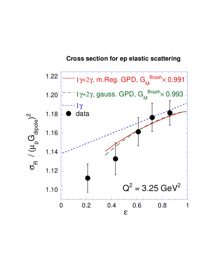
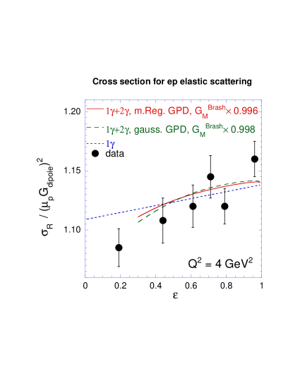
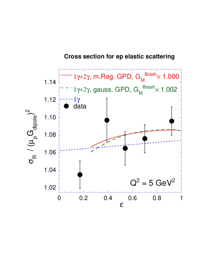
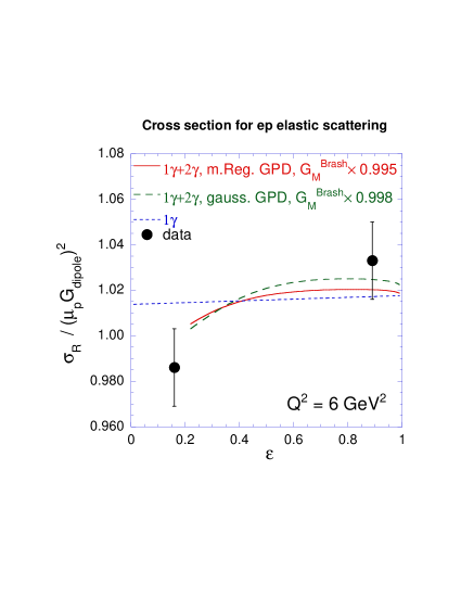
Figure 3: Rosenbluth plots for elastic $ep$ scattering: $\sigma_{R}$ divided by $(\mu_{p}G_{D})^{2}$, with $G_{D}=(1+Q^{2}/0.71)^{-2}$. Dotted curves: Born approximation using $G_{Ep}/G_{Mp}$ from polarization data Jones00 ; Gayou02 . Solid curves: full calculation using the modified Regge GPD, for the kinematical range $-u>M^{2}$. Dashed curves: same as solid curves but using the gaussian GPD. The data are from Ref. Slac94 .

We should remind the reader that $G_{M}^{p}$ is also obtained from the reduced cross section data: the normalization gives $G_{M}^{p}$ and the slope gives $G_{E}^{p}/G_{M}^{p}$. As a starting point we adopt the parametrization for $G_{M}^{p}$, of Ref. Bra02 . The straight dotted curves of Fig. 3 show that the values of $G_{E}^{p}/G_{M}^{p}$ extracted from the polarization experiments are inconsistent with the one-photon exchange analysis of the Rosenbluth data, corrected with just the classic Mo and Tsai radiative corrections MoTsai68 , in the $Q^{2}$ range where data from both methods exist. We then include the $2\gamma$ exchange correction, using the GPD based calculation described in this paper. The plots show the results from both the GPD’s used in our shorter note YCC04 and recorded in the previous section, as well as from the alternative GPD’s also described in the previous section. The results are rather similar.

It is also important to note the non-linearity in the Rosenbluth plot, particularly at the largest $\varepsilon$ values. One sees that over most of the $\varepsilon$ range, the overall slope has become steeper, in agreement with the experimental data. This change in slope is crucial: we see that including the $2\gamma$ exchange allows one to reconcile the polarization transfer and Rosenbluth data.

It is clearly worthwhile to do a global re-analysis of all large $Q^{2}$ elastic data including the $2\gamma$ exchange correction in order to redetermine the values of $G_{E}^{p}$ and $G_{M}^{p}$. For example, in order to best fit the data when including the $2\gamma$ exchange correction, one should slightly change the value of $G_{M}^{p}$ of Ref. Bra02 . A full analysis is beyond the scope of this paper,

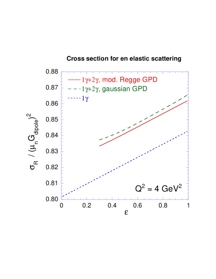
Figure 4: A Rosenbluth plot for elastic $en$ scattering. The curves with the two-photon corrections are plotted only for $-u>M^{2}$. For $G_{M}^{n}$ and $G_{E}^{n}$ we used fits from kubon and madey , respectively. There is little slope change for the neutron case, for reasons noted in the text.

In Fig. 4, we show a similar plot for electron-neutron elastic scattering. Because of a partial cancellation between contributions proportional to $G_{E}^{n}$ and $G_{M}^{n}$, there is little $\varepsilon$ dependence in the corrections, and the slope is not appreciably modified. We took $G_{M}^{n}$ from the fit of kubon ; for $G_{E}^{n}$ we used the fit given in madey .

V.2 Single spin asymmetry

The single spin asymmetry $A_{n}$ or $P_{n}$ is a direct measure of the imaginary part of the $2\gamma$ exchange amplitudes. Our GPD estimate for $A_{n}$ for the proton is shown in the left-hand plot of Fig. 5 as a function of the CM scattering angle for fixed incoming electron lab energy, taken here as $6$ GeV. Also shown is a calculation of $A_{n}$ including the elastic intermediate state only RKR71 . The result, which is nearly the same for either of the two GPD’s that we use, is of order 1%.

Fig. 5 on the right also shows a similar plot of the single spin asymmetry for a neutron target. The predicted asymmetry is of opposite sign, reflecting that the numerically largest term is the one proportional to $G_{M}$. The results are again of order 1% in magnitude, though somewhat larger for the neutron than for the proton.

A precision measurement of $A_{n}$ is planned at JLab AnTodd on a polarized ${}^{3}He$ target; it will provide access to the elastic electron-neutron single-spin asymmetry from two-photon exchange.

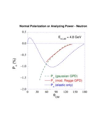
Figure 5: Nucleon analyzing power, which is equal to normal recoil polarization. The elastic contribution (nucleon intermediate state in the two-photon exchange box diagram) is shown by the dotted curve RKR71 . The GPD calculation for the inelastic contribution is shown by the dashed curve for the gaussian GPD, and by the solid curve for the modified Regge GPD. The GPD calculation is cut off in the backward direction at $-u=M^{2}$. In the forward direction the modified Regge GPD result goes down to $Q^{2}=2$ GeV² and the gaussian GPD result to $Q^{2}=M^{2}$.

V.3 Polarization transfers

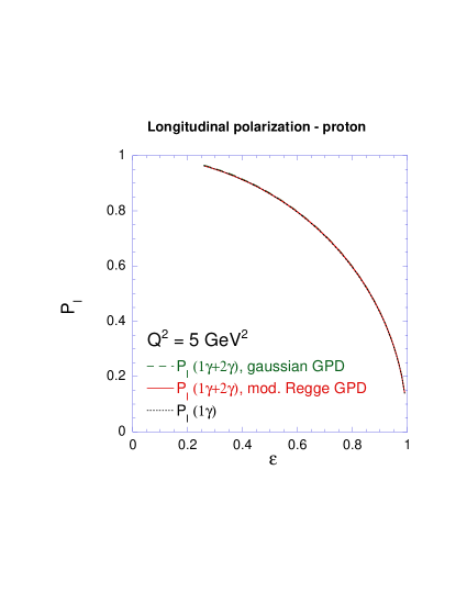
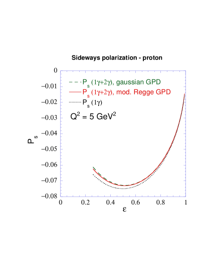
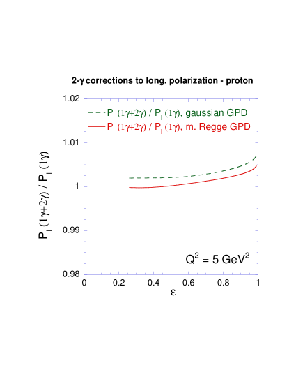
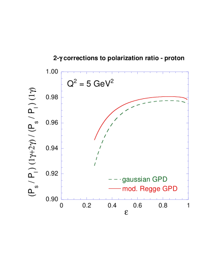
Figure 6: Recoil proton polarization components $P_{s}$ and $P_{l}$ and their ratios relative to the $1\gamma$ exchange results (lower panels) for elastic $ep$ scattering at $Q^{2}$ = 5 GeV². The dotted curves in the upper panels are the Born approximation ($1\gamma$ exchange) results. The solid curves include the $2\gamma$ exchange correction using the GPD calculation, for the kinematical range where both $s,-u>M^{2}$.

The polarization transfer method for measuring the ratio $G_{E}/G_{M}$ depends on measuring outgoing nucleon polarizations $P_{l}$ and $P_{s}$ for polarized incoming electrons. Their ratio is

$${P_{s}\over P_{l}}=-\sqrt{2\epsilon\over\tau(1+\epsilon)}\ {G_{E}\over G_{M}}\ ,$$ (61)

in the one-photon exchange calculation. This also is subject to additional corrections from two-photon exchange. However, the impact of the corrections upon $G_{E}$ is not in any way enhanced, and so one expects and finds that the corrections to $G_{E}$ measured this way are smaller than the corrections to $G_{E}$ coming from the cross section experiments.

Figure 6 shows in the upper two panels the calculated $P_{l}$ and $P_{s}$ for $ep$ scattering with and without the two-photon exchange terms, for 100% right-handed electron polarization and with fixed momentum transfer $Q^{2}=5$ GeV². The two GPD’s were presented in the previous section, and we use again the polarization $G_{E}/G_{M}$ from Gayou02 and $G_{M}$ from Bra02 . The corrections to the longitudinal polarization are quite small, as is seen again in the lower left panel, where the ratio of the full calculation divided by the one-photon exchange calculation is shown. The lower right panel shows the corrections to the $P_{s}/P_{l}$ ratio, given as a ratio again of the full calculation to the one-photon calculation. An experiment to measure the $\varepsilon$-dependence of $P_{s}/P_{l}$ is planned at JLab charles . This will allow a test of the two-photon corrections.

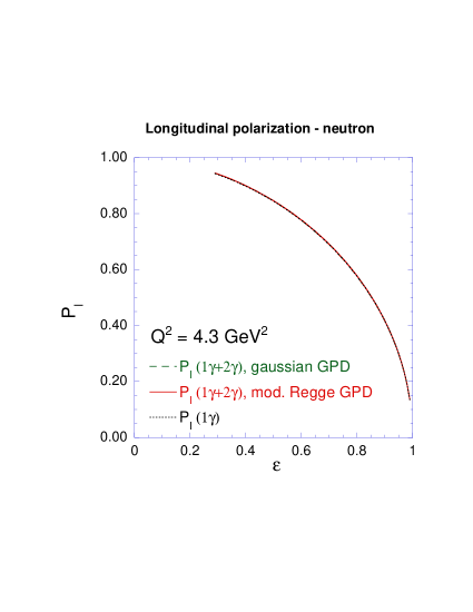
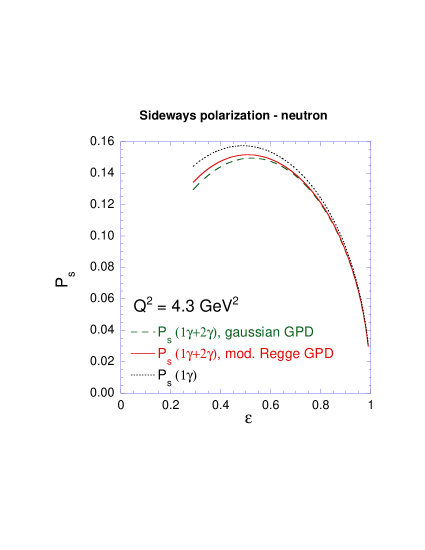
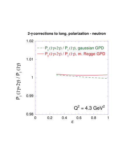
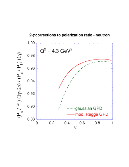
Figure 7: Recoil neutron polarization components $P_{s}$ and $P_{l}$ and their ratios relative to the $1\gamma$ exchange results (lower panels) for elastic $ep$ scattering at $Q^{2}$ = 4.3 GeV². See Fig. 6 for notation.

Figure 7 shows the corresponding plots for the neutron, at a momentum transfer squared of 4.3 GeV². If one needs to choose between the GPD’s, the modified Regge model should be chosen as it gives the better account of the existing data on the form factors, the neutron form factors in particular guidal .

V.4 Positron-proton vs. electron-proton

Positron-proton and electron-proton scattering have the opposite sign for the two-photon corrections relative to the one-photon terms. Hence one expects $e^{+}p$ and $e^{-}p$ elastic scattering to differ by a few percent. Figure 8 shows our results for three different $Q^{2}$ values. These curves are obtained by adding our two-photon box calculation, minus the corresponding part of the soft only calculation in MoTsai68 , to the one-photon calculations; hence, they are meant to be compared to data where the corrections given in MoTsai68 have already been made. Each curve is based on the gaussian GPD and is cut off at low $\varepsilon$ when $-u=M^{2}$. Early data from SLAC are available Mar68 ; more precise data are anticipated from JLab brooks . (Ref. Mar68 used the Meister-Yennie oldyennie soft corrections rather than those of Mo and Tsai. We have checked that for these kinematics the difference between them is smaller than $0.1\%,$ which is negligible compared to the size of the error bars.)

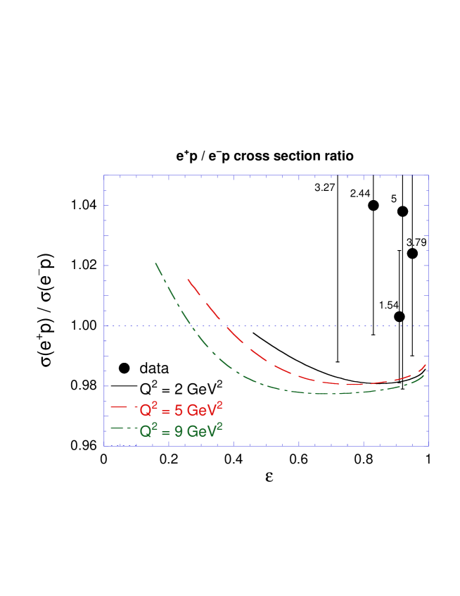
Figure 8: Ratio of $e^{+}/e^{-}$ elastic cross sections on the proton. The GPD calculations for the $2\gamma$ exchange correction are for three fixed $Q^{2}$ values of 2, 5, and 9 GeV², for the kinematical range where $-u$ is above $M^{2}$. Also shown are all known data, from Mar68 , with $Q^{2}$ above 1.5 GeV² (the missing central value is at 1.111). The numbers near the data give $Q^{2}$ for that point in GeV².

V.5 Possibilities at lower $|u|$

In numerical calculations, we used a conservative requirement that the values of the Mandelstam variable $|u|>M^{2}$ in order to apply the partonic description. In a ‘handbag’ mechanism of wide-angle Compton scattering on a proton, such a requirement is needed to enforce high virtuality of the quark line between the two currents, making sure that short light-cone distances dominate. However, our case of electron–quark scattering via two-photon exchange involves 4-dimensional loop integration, and small values of $|u|$ do not necessarily mean that the struck quark has small virtuality. Analyzing the two-photon-exchange loop integral in terms of Sudakov variables one may show that for the backward ($u\to 0$) electron–quark scattering, high virtuality of the quark dominates the loop integral, thereby justifying extension of our approach to the region of small $u$, as long as $s$ and $-t$ remain large. Such an analysis may be found in the literature for the backward-angle electron-muon scattering in QED gglf , and we found our formalism consistent with these early calculations.

V.6 Rosenbluth determinations of $G_{E}/G_{M}$ including 2-photon corrections

Previous Rosenbluth determinations of $G_{E}/G_{M}$ were made using data which had been radiatively corrected using the Mo-Tsai MoTsai68 or comparable oldyennie prescription. Given the work in this paper, we would now say that these corrections are just a part of the total radiative correction. One should also include the hard two-photon corrections.

We present here new Rosenbluth determinations of $G_{E}^{p}/G_{M}^{p}$ using known data but including the two-photon corrections. We used cross section data from Andivahis et al. Slac94 , and made a $\chi^{2}$ fit to the data at each of the five $Q^{2}$ selected using our full calculation and allowing both $G_{M}^{p}$ and $G_{E}^{p}/G_{M}^{p}$ to vary. We included the lowest $\varepsilon$ points in the data by making a linear extrapolation of our calculations from higher $\varepsilon$. (For the record, and for the $\varepsilon$’s in question and to the precision we need, the result is numerically the same as doing our GPD calculation at these $\varepsilon$’s, even though $|u|$ is below $M^{2}$.)

The results are shown in Fig. 9. The figure also shows the results of the polarization transfer measurements, and Rosenbluth results taken from Arrington:2003df , which do not include the hard two-photon corrections. The polarization results also have radiative corrections, but the size of them is, as one has learned from Fig. 6, smaller than the dots of the data points. The solid squares in Fig. 9 show the $G_{E}/G_{M}$ ratios we have extracted with Ref. Slac94 data and the two-photon corrections with the gaussian GPD. The results with the modified Regge GPD are omitted to reduce clutter on the graph; they are about the same as for the gaussian for $Q^{2}$ of 2–3 GeV², and a bit larger at the higher $Q^{2}$.

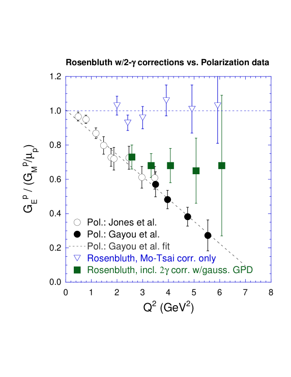
Figure 9: Rosenbluth determinations of $G_{E}/G_{M}$ including the 2-photon corrections. The polarization data is from Jones et al. Jones00 and Gayou et al. Gayou02 , and the Rosenbluth determinations without the two-photon corrections are from Arrington:2003df . The Rosenbluth $G_{E}/G_{M}$ are based on data from Andivahis et al. Slac94 . Some of our points for the Rosenbluth results are slightly offset horizontally for clarity.

For $Q^{2}$ in the 2–3 GeV² range, the $G_{E}/G_{M}$ extracted using the Rosenbluth method including the two-photon corrections agree well with the polarization transfer results. At higher $Q^{2}$, there is at least partial reconciliation between the two methods.

One may comment on the growth of the error bars at higher $Q^{2}$. The calculation with the two-photon contributions includes a lowest order term quadratic in $G_{E}^{p}$ and a correction linear in $G_{E}^{p}$ with opposite sign. The partial cancellation explains the reduced sensitivity to changes in $G_{E}^{p}$.

VI Conclusions

We have studied the effects of two-photon physics for lepton-nucleon elastic scattering. Our main result is a calculation of the two-photon exchange contributions including contributions coming when intermediate particles which are far off shell. The main impediment to performing this calculation is the lack of knowledge of nucleon structure. Here we have used a partonic “handbag” model to express the contributions when both photons are hard in terms of the generalized parton distributions (GPD’s) of the nucleon. The GPD’s also enter calculations of deeply virtual Compton scattering, wide angle Compton scattering, and exclusive meson photoproduction, which are consistent with models for the GPD’s. The calculations which we have presented are valid when $s$, $-u$, and $Q^{2}$ are large, although we have argued in subsection V.5 and Ref. gglf , that the requirement on $-u$ is not compulsory for $eN$ elastic scattering). We have presented our results requiring that the magnitude of each of the invariants is above $M^{2}$.

We have found that in Rosenbluth plots of the differential cross section vs. $\varepsilon$, that the two-photon exchange corrections gives an additional slope which is sufficient to reconcile qualitatively the difference between the Rosenbluth and polarization data. The change in the effective slope in the Rosenbluth plots comes only from corrections where both photons are hard. The reconciliation thus implies only a minor change in the $G_{E}/G_{M}$ ratio as obtained from the polarization data, since those data receive smaller two-photon corrections to $G_{E}/G_{M}$.

Two-photon exchange has additional consequences which could be experimentally observed. For polarizations $P_{s}$ and $P_{l}$, there are two-photon corrections which are small but measurable. For the normal direction, the polarization or analyzing power is zero in the one-photon exchange limit, but the presence of the two-photon exchange amplitude leads to a nonzero effect of ${\cal O}(1\%)$. We also predict a ${\cal O}({\rm few}\%)$ positron-proton/electron-proton asymmetry. The predicted Rosenbluth plot is no longer precisely linear; it acquires a measurable curvature, particularly at high $\varepsilon$.

Thus, in summary, we have shown that the hard two-photon exchange mechanism substantially reconciles the Rosenbluth and polarization transfer measurements of the proton electromagnetic elastic form factors. We have also emphasized that there are important experimentally testable consequences of the two-photon amplitude.

Appendix A Cross section and polarization results in the axial-vector representation

This appendix records the cross section and polarization results using the expansion of the scattering amplitude in the axial-vector representation given by Eq. (10),

$$T_{h,\,\lambda^{\prime}_{N}\lambda_{N}}={e^{2}\over Q^{2}} \Bigg{\{} \bar{u}(k^{\prime},h)\gamma_{\mu}u(k,h)\times\bar{u}(p^{\prime},\lambda^{\prime}_{N})\left[\gamma^{\mu}G^{\prime}_{M}-{P^{\mu}\over M}F^{\prime}_{2}\right]u(p,\lambda_{N})$$ (62)

$$+ \bar{u}(k^{\prime},h)\gamma_{\mu}\gamma_{5}u(k,h)\times\bar{u}(p,\lambda^{\prime}_{N})\,\gamma^{\mu}\gamma^{5}G^{\prime}_{A}\,u(p,\lambda_{N})\ \ \Bigg{\}}\ .$$

A.1 Form factors and observables

The scalar invariants or form factors are in general complex and functions of two variables. We also define

$$G^{\prime}_{E}\equiv G^{\prime}_{M}-(1+\tau)F^{\prime}_{2}\ .$$ (63)

The relations between the present scalar invariants and the ones used in most of the text follow from Eq. (11) and are

$$G^{\prime}_{M} = \tilde{G}_{M}+{s-u\over 4M^{2}}\tilde{F}_{3}$$

$$F^{\prime}_{2} = \tilde{F}_{2}$$

$$G^{\prime}_{A} = -\tau\tilde{F}_{3}$$

$$G^{\prime}_{E} = \tilde{G}_{E}+{s-u\over 4M^{2}}\tilde{F}_{3}\ .$$ (64)

The invariants may be separated into parts coming from one-photon exchange and parts from two- or more-photon exchange,

$$G^{\prime}_{M} = G_{M}+\delta G^{\prime}_{M}\ ,$$

$$G^{\prime}_{E} = G_{E}+\delta G^{\prime}_{E}\ ,$$

$$G^{\prime}_{A} = \delta G^{\prime}_{A}\ ,$$ (65)

where $G_{M}(Q^{2})$ and $G_{E}(Q^{2})$ are the usual magnetic and electric form factors, defined from matrix elements of the electromagnetic current and real for spacelike $Q^{2}$. The quantities $\delta G^{\prime}_{M}$, $\delta G^{\prime}_{E}$, and $G^{\prime}_{A}$ are ${\cal O}(e^{2})$ relative to $G_{M}$ or $G_{E}$.

The reduced cross section in Eq. (14) is

$$\sigma_{R}=|G^{\prime}_{M}|^{2}+{\varepsilon\over\tau}|G^{\prime}_{E}|^{2}+2\sqrt{(1+\tau)(1-\varepsilon^{2})\over\tau}\ G_{M}{\,\cal R\,}(G^{\prime}_{A})+{\cal O}(e^{4})\ .$$ (66)

The polarizations of the outgoing nucleons or analyzing powers of the target nucleons are

$$P_{n} = A_{n}=\sqrt{\frac{2\,\varepsilon\,(1+\varepsilon)}{\tau}}\,\,\frac{1}{\sigma_{R}}\left\{{\cal I}(G^{\prime*}_{E}G^{\prime}_{M})+\sqrt{{1+\tau\over\tau}\cdot{1-\varepsilon\over 1+\varepsilon}}\,G_{E}\,{\cal I}(G^{\prime}_{A})+{\cal O}(e^{4})\right\}\,,$$

$$P_{s} = A_{s}=-\,P_{e}\sqrt{\frac{2\varepsilon(1-\varepsilon)}{\tau}}\,\frac{1}{\sigma_{R}}\left\{{\,\cal R\,}\left(G^{\prime*}_{E}G^{\prime}_{M}\right)+\sqrt{{1+\tau\over\tau}\cdot{1+\varepsilon\over 1-\varepsilon}}\,G_{E}{\,\cal R\,}\left(G^{\prime}_{A}\right)+{\cal O}(e^{4})\right\}\,,$$

$$P_{l} = -A_{l}=P_{e}\,\frac{1}{\sigma_{R}}\left\{\sqrt{1-\varepsilon^{2}}\,|G^{\prime}_{M}|^{2}+2\sqrt{{1+\tau\over\tau}}\,G_{M}{\,\cal R}(G^{\prime}_{A})+{\cal O}(e^{4})\right\}\,.$$ (67)

The only single spin asymmetry is $P_{n}$ or $A_{n}$. Further, $P_{n}$ or $A_{n}$ is zero if there be only one-photon exchange, so observation of a non-zero value is definitive evidence for multiple-photon exchange. Polarizations $P_{s}$ or $P_{l}$ are double polarizations. The expressions for them are proportional to the electron longitudinal polarization $P_{e}$ (with, e.g., $P_{e}=1$ if $h=+1/2$).

A.2 Electron-quark elastic scattering amplitudes

The two-photon part of electron-quark elastic scattering is given by

$$H_{h,\lambda} = \frac{(e\,e_{q})^{2}}{Q^{2}}\Big{\{}g_{M}\ \bar{u}(k^{\prime},h)\gamma_{\mu}u(k,h)\,\cdot\,\bar{u}(p^{\prime}_{q},\lambda)\gamma^{\mu}u(p_{q},\lambda)$$ (68)

$$\qquad+\ g_{A}^{(2\gamma)}\ \bar{u}(k^{\prime},h)\gamma_{\mu}\gamma_{5}u(k,h)\,\cdot\,\bar{u}(p^{\prime}_{q},\lambda)\gamma^{\mu}\gamma^{5}u(p_{q},\lambda)\Big{\}}$$

$$= \frac{(e\,e_{q})^{2}}{Q^{2}}\Big{\{}\Big{(}\hat{s}-\hat{u}-(2h)(2\lambda)t\Big{)}\,g_{M}+\Big{(}(2h)(2\lambda)(\hat{s}-\hat{u})-t\Big{)}g_{A}^{(2\gamma)}\Big{\}}\ ,$$

when the electrons and quarks are both massless. The theorem of Eq. (11) relates

$$g_{M} = \tilde{f}_{1}+{\hat{s}-\hat{u}\over 4}\tilde{f}_{3}\ ,$$

$$g_{A}^{(2\gamma)} = {t\over 4}\tilde{f}_{3}\ .$$ (69)

We split the two-photon part of $g_{M}$ into a hard and soft part, $g_{M}^{(2\gamma)}=g_{M}^{\,soft}+g_{M}^{\,hard}$, using the prescription of Grammer and Yennie grammer , and have

$${\cal R}\left(g_{M}^{\,soft}\right) = {\alpha\over\pi}\left\{\ln\left(\frac{\lambda^{2}}{\sqrt{-\hat{s}\hat{u}}}\right)\ln\left(\frac{\hat{s}}{-\hat{u}}\right)+\frac{\pi^{2}}{2}\right\}\ ,$$

$${\cal I}\left(g_{M}^{\,soft}\right) = \alpha\ln\left(\hat{s}\over\lambda^{2}\right)\ ,$$

$${\cal R}\left(g_{M}^{\,hard}\right) = {\alpha\over 4\pi}\Bigg{\{}{-t\over\hat{u}}\ln\left(\hat{s}\over-t\right)+{t\over\hat{s}}\ln\left(\hat{u}\over t\right)$$

$$\qquad+\,{\hat{s}^{2}+3\hat{u}^{2}\over 2\hat{u}^{2}}\ln^{2}\left(\hat{s}\over-t\right)-{3\hat{s}^{2}+\hat{u}^{2}\over 2\hat{s}^{2}}\left(\ln^{2}\left(\hat{u}\over t\right)+\pi^{2}\right)\Bigg{\}}\ ,$$

$${\cal I}\left(g_{M}^{\,hard}\right) = -\alpha\left\{{\hat{s}^{2}+3\hat{u}^{2}\over 4\hat{u}^{2}}\ln\left(\hat{s}\over-t\right)-{t\over 4\hat{u}}\right\}\ ,$$

$${\cal R}\left(g_{M}^{(2\gamma)}\right) = \frac{\alpha}{4\pi}\,\frac{t}{\hat{s}\,\hat{u}}\,\left\{\hat{s}\,\ln\left(\frac{\hat{s}}{-t}\right)+\hat{u}\,\ln\left(\frac{\hat{u}}{t}\right)+\frac{\hat{s}-\hat{u}}{2}\left[\frac{\hat{s}}{\hat{u}}\ln^{2}\left(\frac{\hat{s}}{-t}\right)-\frac{\hat{u}}{\hat{s}}\ln^{2}\left(\frac{\hat{u}}{t}\right)-\frac{\hat{u}}{\hat{s}}\pi^{2}\right]\right\}\ ,$$

$${\cal I}\left(g_{M}^{(2\gamma)}\right) = -\alpha\,\frac{t}{4\hat{u}}\,\left\{\frac{\hat{s}-\hat{u}}{\hat{u}}\ln\left(\frac{\hat{s}}{-t}\right)+1\right\}\ .$$ (70)

A.3 Embedding

The nucleon form factors are given in terms of the quark-level amplitudes and generalized parton distributions by

$$\delta G^{\prime(hard)}_{M} = {1+\varepsilon\over 2\varepsilon}A-{1-\varepsilon\over 2\varepsilon}C\ ,$$

$$\delta G^{\prime(hard)}_{E} = \sqrt{1+\varepsilon\over 2\varepsilon}B\ ,$$

$$\delta G^{\prime(hard)}_{A} = {t\over s-u}{1+\varepsilon\over 2\varepsilon}\left(A-C\right)\ .$$ (71)

Quantities $A$, $B$, and $C$ are the same as in the text, but now written as

$$A = \int_{-1}^{1}\frac{dx}{x}\ {(\hat{s}-\hat{u})g_{M}^{\,hard}-tg_{A}^{(2\gamma)}\over s-u}\sum_{q}e_{q}^{2}\,\left(H^{q}+E^{q}\right),$$

$$B = \int_{-1}^{1}\frac{dx}{x}\ {(\hat{s}-\hat{u})g_{M}^{\,hard}-tg_{A}^{(2\gamma)}\over s-u}\sum_{q}e_{q}^{2}\,\left(H^{q}-\tau E^{q}\right),$$

$$C = \int_{-1}^{1}\frac{dx}{x}\ {(\hat{s}-\hat{u})g_{A}^{(2\gamma)}-tg_{M}^{\,hard}\over-t}\,\mathrm{sgm}(x)\,\sum_{q}e_{q}^{2}\,\tilde{H}^{q},$$ (72)

and it is understood in Eq. (A.3) that the partonic amplitude $g_{M}$ has its soft part removed.

Appendix B Quark mass sensitivity

B.1 Kinematics, and imaginary parts of the hard amplitudes

We have until now set the quark mass to zero.

To investigate how severe this approximation is, we will examine the effect of restoring the quark mass for the analyzing power calculations, though still keeping only the quark chirality conserving amplitudes. There are three modifications. The expressions for $\hat{s}$ and $\hat{u}$ become

$$\hat{s}=\frac{(x+\eta)^{2}}{4\,x\,\eta}\,Q^{2}+\frac{x+\eta}{x}m_{q}^{2}\,,\qquad\hat{u}=-\frac{(x-\eta)^{2}}{4\,x\,\eta}\,Q^{2}+\frac{x-\eta}{x}m_{q}^{2}\,,$$ (73)

where $m_{q}$ is the effective quark mass. The general electron-quark scattering amplitude, Eq. (22), should have another term with a scalar function that we may call $\tilde{f}_{2}$ in analogy with the expansion of the electron-nucleon amplitude given in Eq. (II). However, this term flips quark helicities, and presently the formalism for embedding quark amplitudes into the nucleon using GPD’s involves only the non-chirality flip GPD’s. There is neither theoretical development nor experimental information regarding chirality flip GPD’s, and so we shall ignore $\tilde{f}_{2}$ as well as helicity flip parts of other amplitudes. Including the quark mass leads to a modification of the hard scattering amplitudes so that

$$\frac{1}{2}\left[H_{h,\,+\frac{1}{2}}^{hard}+H_{h,\,-\frac{1}{2}}^{hard}\right] \stackrel{{\scriptstyle(m_{q}=0)}}{{=}} \frac{e^{2}}{Q^{2}}\left\{\left[\hat{s}-\hat{u}\right]\tilde{f}_{1}^{hard}-\hat{s}\hat{u}\tilde{f}_{3}\right\}$$ (74)

$$\stackrel{{\scriptstyle\to}}{{=}} \frac{e^{2}}{Q^{2}}\left\{\left[\hat{s}-\hat{u}-\frac{2m_{q}^{2}}{\hat{s}-m_{q}^{2}}Q^{2}\right]\tilde{f}_{1}^{hard}+\left[m_{q}^{4}-\hat{s}\hat{u}\right]\tilde{f}_{3}\right\}\ ,$$

within the quantities $A$ and $B$ ($C$ is not needed for the analyzing power), and

$${\cal I}\left(\tilde{f}_{1}^{hard}\right) = -\frac{e^{2}}{4\pi}\left\{\frac{\frac{1}{2}\hat{s}Q^{2}}{\hat{s}Q^{2}-\left(\hat{s}-m_{q}^{2}\right)^{2}}\,\ln\left[\frac{\left(\hat{s}-m_{q}^{2}\right)^{2}}{\hat{s}Q^{2}}\right]+\frac{\hat{s}+m_{q}^{2}}{2\hat{s}}\right\},$$

$${\cal I}\left(\tilde{f}_{3}\right) = -\frac{e^{2}}{4\pi}\,\frac{\hat{s}-m_{q}^{2}}{\hat{s}Q^{2}-\left(\hat{s}-m_{q}^{2}\right)^{2}}$$ (75)

$$\times\ \left\{\frac{(\hat{s}-\hat{u})(\hat{s}-m_{q}^{2})}{\hat{s}Q^{2}-\left(\hat{s}-m_{q}^{2}\right)^{2}}\,\ln\left[\frac{\left(\hat{s}-m_{q}^{2}\right)^{2}}{\hat{s}Q^{2}}\right]+\frac{\hat{s}+m_{q}^{2}}{\hat{s}}\right\}\,.$$

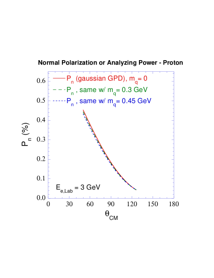
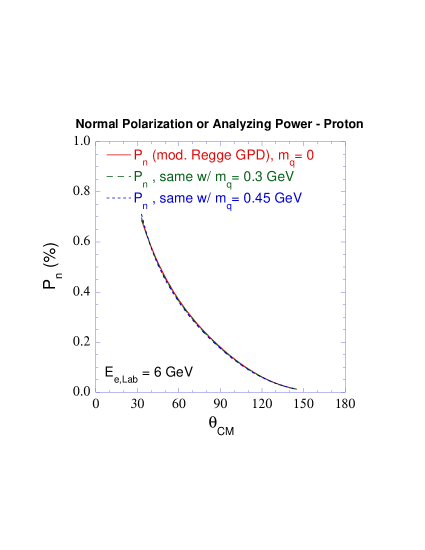
Figure 10: Quark mass correction plots for the analyzing power or normal polarization, for fixed electron incoming lab energies of 3 and 6 GeV.

The results for the analyzing power $A_{n}$ when including quark masses in the quark helicity conserving amplitudes are shown in Fig. 10 for quark masses 300 MeV and 450 MeV. The effects are clearly not large.

B.2 Real parts of hard two-photon exchange amplitudes with finite quark mass

When the quark mass is not zero, we have

$${\cal R}\left(\tilde{f}_{1}^{hard}\right) = \frac{e^{2}}{4\pi^{2}}\cdot\left\{\left[\ln\left(\frac{\sqrt{(\hat{s}-m_{q}^{2})|\hat{u}-m_{q}^{2}|}}{Q^{2}}\right)\,+\,\frac{1}{2}\right]\cdot\ln\left|\frac{\hat{s}-m_{q}^{2}}{\hat{u}-m_{q}^{2}}\right|\right.$$ (76)

$$+\frac{m_{q}^{2}}{2}\left[\frac{1}{\hat{s}}\ln\left(\frac{\hat{s}-m_{q}^{2}}{m_{q}^{2}}\right)-\frac{1}{\hat{u}}\ln\left|\frac{\hat{u}-m_{q}^{2}}{m_{q}^{2}}\right|\right]$$

$$+\frac{1}{2}\frac{Q^{2}(\hat{s}-\hat{u})}{(m_{q}^{4}-\hat{s}\hat{u})}\left[\,\frac{\pi^{2}}{2}+\frac{1}{4}\ln^{2}\left(\frac{m_{q}^{2}}{Q^{2}}\right)\right]-\frac{1}{2}\ln^{2}\left(\frac{\hat{s}-m_{q}^{2}}{Q^{2}}\right)+\frac{1}{2}\ln^{2}\left|\frac{\hat{u}-m_{q}^{2}}{Q^{2}}\right|$$

$$+\frac{1}{2}\frac{(\hat{s}-\hat{u})(\hat{s}+\hat{u})}{(m_{q}^{4}-\hat{s}\hat{u})}\,\frac{1}{\chi}$$

$$\times\left[\,L\left(\frac{2}{1+\chi}\right)-\frac{\pi^{2}}{2}+\frac{1}{2}\ln\left(\frac{m_{q}^{2}}{Q^{2}}\right)\ln\left(\frac{1+\chi}{-1+\chi}\right)+\frac{1}{4}\ln^{2}\left(\frac{1+\chi}{-1+\chi}\right)\right]$$

$$-\frac{1}{2}\frac{Q^{2}\,\hat{s}}{(m_{q}^{4}-\hat{s}\hat{u})}\left[L\left(\frac{\hat{s}-m_{q}^{2}}{\hat{s}}\right)+\frac{1}{2}\ln^{2}\left(\frac{\hat{s}-m_{q}^{2}}{\hat{s}}\right)+\frac{1}{2}\ln^{2}\left(\frac{\hat{s}-m_{q}^{2}}{Q^{2}}\right)\right]$$

$$+\frac{1}{2}\frac{Q^{2}\,\hat{u}}{(m_{q}^{4}-\hat{s}\hat{u})}\left[-L\left(\frac{\hat{u}}{\hat{u}-m_{q}^{2}}\right)+\frac{5\pi^{2}}{6}+\frac{1}{2}\ln^{2}\left|\frac{\hat{u}-m_{q}^{2}}{Q^{2}}\right|\right]\Bigg{\}}\,,$$

and

$${\cal R}\left(\tilde{f}_{3}\right) = -\frac{e^{2}}{4\pi^{2}}\frac{1}{(m_{q}^{4}-\hat{s}\hat{u})}\cdot\left\{\frac{\hat{s}^{2}-m_{q}^{4}}{\hat{s}}\ln\left(\frac{\hat{s}-m_{q}^{2}}{Q^{2}}\right)+\frac{\hat{u}^{2}-m_{q}^{4}}{\hat{u}}\ln\left|\frac{\hat{u}-m_{q}^{2}}{Q^{2}}\right|\right.$$ (77)

$$+\frac{(\hat{s}-\hat{u})^{2}Q^{2}}{(m_{q}^{4}-\hat{s}\hat{u})}\left[\frac{\pi^{2}}{3}+\frac{1}{4}\ln^{2}\left(\frac{m_{q}^{2}}{Q^{2}}\right)\right]+m_{q}^{2}\left(-2+\frac{m_{q}^{2}(\hat{s}+\hat{u})}{\hat{s}\hat{u}}\right)\ln\left(\frac{m_{q}^{2}}{Q^{2}}\right)$$

$$+\frac{(\hat{s}-\hat{u})^{2}(\hat{s}+\hat{u})+4m_{q}^{2}(m_{q}^{4}-\hat{s}\hat{u})}{(m_{q}^{4}-\hat{s}\hat{u})}\,\frac{1}{\chi}$$

$$\times\left[\,L\left(\frac{2}{1+\chi}\right)-\frac{\pi^{2}}{2}+\frac{1}{2}\ln\left(\frac{m_{q}^{2}}{Q^{2}}\right)\ln\left(\frac{1+\chi}{-1+\chi}\right)+\frac{1}{4}\ln^{2}\left(\frac{1+\chi}{-1+\chi}\right)\right]$$

$$+\frac{(\hat{s}-\hat{u})(\hat{s}-m_{q}^{2})^{2}}{(m_{q}^{4}-\hat{s}\hat{u})}\left[-L\left(\frac{\hat{s}-m_{q}^{2}}{\hat{s}}\right)+\frac{\pi^{2}}{6}-\frac{1}{2}\ln^{2}\left(\frac{\hat{s}-m_{q}^{2}}{\hat{s}}\right)-\frac{1}{2}\ln^{2}\left(\frac{\hat{s}-m_{q}^{2}}{Q^{2}}\right)\right]$$

$$+\frac{(\hat{s}-\hat{u})(\hat{u}-m_{q}^{2})^{2}}{(m_{q}^{4}-\hat{s}\hat{u})}\left.\left[-L\left(\frac{\hat{u}}{\hat{u}-m_{q}^{2}}\right)+\frac{2\pi^{2}}{3}+\frac{1}{2}\ln^{2}\left|\frac{\hat{u}-m_{q}^{2}}{Q^{2}}\right|\right]\right\},$$

where $\hat{s}$ and $\hat{u}$ were given in Eq. (73), and

$$\chi\equiv\sqrt{1+4m_{q}^{2}/Q^{2}}\,.$$ (78)

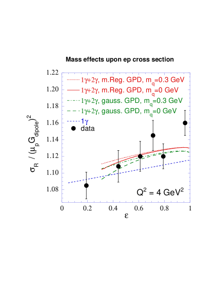
Figure 11: Quark mass correction plot for the reduced cross section. The curves are as labeled. In this plot, all curves have $G_{M}$ set to 0.99 times the Brash et al. value Bra02 . The data is from Slac94 .

The effect of the quark mass corrections upon the reduced cross section is shown in Fig. 11 for $Q^{2}=4$ GeV². One sees from Fig. 11 that the quark mass effects mainly influence our result at small values of $\varepsilon$, where $|u|$ becomes small. They show the theoretical error on our calculation in this region. A full calculation also requires quantifying the effect of the cat’s ears diagrams. A study of such corrections is clearly worthwhile for a future work, both for two-photon exchange amplitudes and for wide-angle Compton scattering.

References

- (1) M. K. Jones et al. [Jefferson Lab Hall A Collaboration], Phys. Rev. Lett. 84, 1398 (2000) [arXiv:nucl-ex/9910005].
- (2) O. Gayou et al. [Jefferson Lab Hall A Collaboration], Phys. Rev. Lett. 88, 092301 (2002) [arXiv:nucl-ex/0111010].
- (3) A.I. Akhiezer, L.N. Rosentsweig, I.M. Shmushkevich, Sov. Phys. JETP 6, 588 (1958); J. Scofield, Phys. Rev. 113, 1599 (1959); ibid. 141, 1352 (1966); N. Dombey, Rev. Mod. Phys. 41, 236 (1969); A. I. Akhiezer and M. P. Rekalo, Sov. J. Part. Nucl. 4, 277 (1974); R. G. Arnold, C. E. Carlson and F. Gross, Phys. Rev. C 23, 363 (1981).
- (4) M. E. Christy et al. [E94110 Collaboration], Phys. Rev. C 70, 015206 (2004) [arXiv:nucl-ex/0401030].
- (5) J. Arrington [JLab E01-001 Collaboration], arXiv:nucl-ex/0312017.
- (6) L. Andivahis et al., Phys. Rev. D 50, 5491 (1994).
- (7) P. A. M. Guichon and M. Vanderhaeghen, Phys. Rev. Lett. 91, 142303 (2003) [arXiv:hep-ph/0306007].
- (8) L. W. Mo and Y. S. Tsai, Rev. Mod. Phys. 41, 205 (1969).
- (9) N. Meister and D. R. Yennie, Phys. Rev. 130, 1210 (1963).
- (10) L. C. Maximon and J. A. Tjon, Phys. Rev. C 62, 054320 (2000) [arXiv:nucl-th/0002058].
- (11) A. Afanasev, I. Akushevich and N. Merenkov, Phys. Rev. D 64, 113009 (2001) [arXiv:hep-ph/0102086].
- (12) P. G. Blunden, W. Melnitchouk and J. A. Tjon, Phys. Rev. Lett. 91, 142304 (2003) [arXiv:nucl-th/0306076].
- (13) Y. C. Chen, A. Afanasev, S. J. Brodsky, C. E. Carlson and M. Vanderhaeghen, Phys. Rev. Lett. 93, 122301 (2004) [arXiv:hep-ph/0403058].
- (14) S. J. Brodsky and G. P. Lepage, Phys. Rev. D 24, 1808 (1981).
- (15) T. C. Brooks and L. J. Dixon, Phys. Rev. D 62, 114021 (2000) [arXiv:hep-ph/0004143]; M. Vanderhaeghen, P. A. M. Guichon and J. Van de Wiele, Nucl. Phys. A 622, 144C (1997); and private communication.
- (16) S. J. Brodsky, F. E. Close and J. F. Gunion, Phys. Rev. D 8, 3678 (1973).
- (17) M. Damashek and F. J. Gilman, Phys. Rev. D 1, 1319 (1970).
- (18) S. J. Brodsky, F. E. Close and J. F. Gunion, Phys. Rev. D 5, 1384 (1972).
- (19) M. Diehl, T. Feldmann, R. Jakob and P. Kroll, Phys. Lett. B 460, 204 (1999) [arXiv:hep-ph/9903268]; Eur. Phys. J. C 8, 409 (1999) [arXiv:hep-ph/9811253].
- (20) A. V. Radyushkin, Phys. Rev. D 58, 114008 (1998) [arXiv:hep-ph/9803316].
- (21) H. W. Huang, P. Kroll and T. Morii, Eur. Phys. J. C 23, 301 (2002) [Erratum-ibid. C 31, 279 (2003)] [arXiv:hep-ph/0110208].
- (22) J. F. Gunion and R. Blankenbecler, Phys. Rev. D 3, 2125 (1971). Dominance of double-scattering diagrams at large angles in the deuteron has been often noted; see, e.g., C. E. Carlson, Phys. Rev. C 2, 1224 (1970).
- (23) I. A. Qattan et al., arXiv:nucl-ex/0410010.
- (24) Allan S. Krass, Phys. Rev. 125, 2172 (1962).
- (25) R. Ent, B. W. Filippone, N. C. R. Makins, R. G. Milner, T. G. O’Neill and D. A. Wasson, Phys. Rev. C 64, 054610 (2001).
- (26) M.L. Goldberger, Y. Nambu and R. Oehme, Ann. of Phys. 2, 226 (1957).
- (27) A. De Rujula, J. M. Kaplan and E. De Rafael, Nucl. Phys. B 35, 365 (1971).
- (28) A. Afanasev, I. Akushevich, and N. P. Merenkov, arXiv:hep-ph/0208260; M. Gorchtein, P. A. M. Guichon and M. Vanderhaeghen, Nucl. Phys. A 741, 234 (2004) [arXiv:hep-ph/0404206]; L. Dixon and M. Schreiber, Phys. Rev. D 69, 113001 (2004) [arXiv:hep-ph/0402221]; B. Pasquini and M. Vanderhaeghen, Phys. Rev. C 70, 045206 (2004) [arXiv:hep-ph/0405303]; A. V. Afanasev and N. P. Merenkov, Phys. Lett. B 599, 48 (2004) [arXiv:hep-ph/0407167] and Phys. Rev. D 70, 073002 (2004) [arXiv:hep-ph/0406127].
- (29) S. P. Wells et al. [SAMPLE collaboration], Phys. Rev. C 63, 064001 (2001) [arXiv:nucl-ex/0002010]; F. E. Maas et al., arXiv:nucl-ex/0410013.
- (30) P. Van Nieuwenhuizen, Nucl. Phys. B 28, 429 (1971).
- (31) G. J. Grammer and D. R. Yennie, Phys. Rev. D 8, 4332 (1973).
- (32) V. V. Bytev, E. A. Kuraev and B. G. Shaikhatdenov, J. Exp. Theor. Phys. 96, 193 (2003) [Zh. Eksp. Teor. Fiz. 123, 224 (2003)]; J. Exp. Theor. Phys. 95, 404 (2002) [Zh. Eksp. Teor. Fiz. 122, 472 (2002)] [arXiv:hep-ph/0203127].
- (33) I. B. Khriplovich, Yad. Fiz. 17 (1973) 576; R. W. Brown, K. O. Mikaelian, V. K. Cung and E. A. Paschos, Phys. Lett. B 43, 403 (1973).
- (34) A.O. Barut and C. Fronsdal, Phys. Rev. 120, 1871 (1960).
- (35) For a general discussion, see S. J. Brodsky and J. R. Primack, Annals Phys. 52, 315 (1969).
- (36) S. D. Drell and T. M. Yan, Phys. Rev. Lett. 24, 181 (1970).
- (37) S. J. Brodsky, F. E. Close and J. F. Gunion, Phys. Rev. D 5, 1384 (1972).
- (38) K. Goeke, M. V. Polyakov and M. Vanderhaeghen, Prog. Part. Nucl. Phys. 47, 401 (2001) [arXiv:hep-ph/0106012].
- (39) A. D. Martin, R. G. Roberts, W. J. Stirling and R. S. Thorne, Phys. Lett. B 531, 216 (2002) [arXiv:hep-ph/0201127].
- (40) E. Leader, A. V. Sidorov and D. B. Stamenov, Eur. Phys. J. C 23, 479 (2002) [arXiv:hep-ph/0111267].
- (41) F. Yuan, Phys. Rev. D 69, 051501 (2004) [arXiv:hep-ph/0311288].
- (42) M. Guidal, M. Polyakov, A. Radyushkin, and M. Vanderhaeghen, arXiv:hep-ph/0410251.
- (43) E. J. Brash, A. Kozlov, S. Li and G. M. Huber, Phys. Rev. C 65, 051001 (2002) [arXiv:hep-ex/0111038].
- (44) G. Kubon et al., Phys. Lett. B 524, 26 (2002) [arXiv:nucl-ex/0107016].
- (45) R. Madey et al. [E93-038 Collaboration], Phys. Rev. Lett. 91, 122002 (2003) [arXiv:nucl-ex/0308007]; see also G. Warren et al. [Jefferson Lab E93-026 Collaboration], Phys. Rev. Lett. 92, 042301 (2004) [arXiv:nucl-ex/0308021].
- (46) JLab experiment E-05-015, spokespersons T. Averett, J.P. Chen, X. Jiang.
- (47) JLab experiment E-04-019, spokespersons R. Gilman, L. Pentchev, C. Perdrisat, and R. Suleiman.
- (48) J. Mar et al., Phys. Rev. Lett. 21, 482 (1968).
- (49) Jefferson Lab experiment E-04-116; contact person, W. Brooks.
- (50) V. G. Gorshkov, V. N. Gribov, L. N. Lipatov, and G. V. Frolov, Sov. J. Nucl. Phys. 6, 95 (1968) [Yad. Fiz. 6, 129 (1967)]; also in V. B. Berestetskii, E. M. Lifshitz, and L. P. Pitaevskii, Quantum Electrodynamics, Course of Theoretical Physics, Vol. 4, Second edition (Pergamon Press, Oxford and New York, 1982), pp. 616ff.
- (51) J. Arrington, Phys. Rev. C 68, 034325 (2003) [arXiv:nucl-ex/0305009].