Abstract

New preliminary combined results from the LEP experiments on searches for the Higgs boson beyond the Standard Model are presented. The new determination of the top quark mass at the Tevatron in 2004 influences the interpretations of the LEP results in both, the Standard Model, and the Minimal Supersymmetric extension of the Standard Model. Higgs boson physics will also be a major research area at the future Linear Collider. A review including new preliminary results on the potential for precision measurements is given.

The LEP experiments took data between August 1989 and November 2000 at center-of-mass energies first around the Z resonance (LEP-1) and from 1996 up to 209 GeV (LEP-2). In 2000 most data was taken around 206 GeV. The LEP accelerator operated very successfully and a total luminosity of ${\cal L}=2461$ pb^-1 was accumulated at LEP-2 energies. Data-taking ended on 3 November 2000, although some data excess was observed in searches for the Standard Model (SM) Higgs boson with 115 GeV mass. In the following sections, these aspects are addressed: 1) SM candidates and mass limits; 2) coupling limits; 3) the Minimal Supersymmetric extension of the SM (MSSM): dedicated searches, three-neutral-Higgs-boson hypothesis, benchmark and general scan mass limits; 4) CP-violating models; 5) invisible Higgs boson decays; 6) neutral Higgs bosons in the general two-doublet Higgs model; 7) Yukawa Higgs boson processes $\rm b\bar{b}h$ and $\rm b\bar{b}A$; 8) singly-charged Higgs bosons; 9) doubly-charged Higgs bosons; 10) fermiophobic Higgs boson decays $\rm h\mbox{$\rightarrow$}WW,ZZ,\gamma\gamma$; 11) uniform and stealthy Higgs boson scenarios; 12) summary of LEP limits; 13) the International Linear Collider (ILC); 14) SM Higgs physics; 15) beyond the SM.

While the results from Standard Model Higgs boson searches are final [1], the results of searches in extended models are mostly preliminary [2]. Limits are given at 95% CL. The Linear Collider aspects are based on Refs. [3, 4].

1 SM Candidates and Mass Limits

From precision electro-weak measurements, the Higgs boson of the SM has a stringent upper mass limit as shown in Fig. 1 (left plot). The preferred value for the SM Higgs boson mass is 114 GeV. This value increased due to the new top mass measurements [5] and it is now very close to mass limit from direct searches. Including both the experimental and the theoretical uncertainties, the mass of the SM Higgs boson is lower than about 260 GeV (one-sided 95% upper CL). The figure shows also the reconstructed mass of the Higgs boson candidates for a 115 GeV Higgs boson hypothesis. In addition, the observed SM Higgs boson mass limit and the expected limit for a background-only hypothesis are shown.

\includegraphics[scale={0.26}]{s04_blueband.eps}

\includegraphics[scale={0.26}]{fig5b.eps}

\includegraphics[scale={0.26}]{fig9.eps}

Figure 1: Left: $\Delta\chi^{2}=\chi^{2}-\chi^{2}_{\rm min}$ vs. Higgs boson mass. The band represents an estimate of the theoretical errors due to higher order corrections. The dashed curves reflect the evaluation for different $\Delta(\alpha_{\rm had})$. Center: reconstructed mass of SM Higgs boson candidates for tight selection cuts. Right: SM Higgs boson mass limit. The 1$\sigma$ and 2$\sigma$ error bands on the expected limit for background are indicated (shaded areas).

2 Coupling Limits

Figure 2 shows coupling limits assuming the Higgs boson decays with SM branching fractions and a SM production rate reduced by $\xi^{2}=(g_{\rm HZZ}/g_{\rm HZZ}^{\rm SM})^{2}$. Coupling limits are also presented for b-quark and $\tau$-lepton decay modes.

\includegraphics[scale={0.26}]{fig10a.eps}

\includegraphics[scale={0.26}]{fig10b.eps}

\includegraphics[scale={0.26}]{fig10c.eps}

Figure 2: Coupling limits. Left: SM decay mode. Center: b-quark decay mode. Right: $\tau$-lepton decay mode. The 1$\sigma$ and 2$\sigma$ error bands on the expected limit for background are indicated (shaded areas).

In searches for flavor-independent hadronic Higgs boson decays, Fig. 3 (left and center plot) shows no indication of a signal for the process $\rm hZ\mbox{$\rightarrow$}q\bar{q}\ell^{+}\ell^{-}$ above the $\rm ZZ\mbox{$\rightarrow$}q\bar{q}\ell^{+}\ell^{-}$ background. The figure shows also combined LEP limits. Remarkably, these mass limits for flavor-blind hadronic decays are close to the SM decay mode limits. Figure 4 (left and center plot) shows results from a related analysis for flavor-independent hadronic Higgs boson decays. The data agrees well with the expected background from W and Z production and resulting limits are shown. Anomalous couplings to the Higgs boson can be parametrized with $\xi$, $d,~{}{d_{\rm B}},~{}{\Delta g_{1}^{{\mathrm{Z}}}},~{}{\Delta\kappa_{\gamma}}$. In addition to the $\xi$ limits, the parameters $d,~{}{d_{\rm B}},~{}{\Delta g_{1}^{{\mathrm{Z}}}},~{}{\Delta\kappa_{\gamma}}$ are constrained as shown in Fig. 4 (right plot).

\includegraphics[width=136.5746pt,clip]{d_qqee_new.eps}

\includegraphics[width=136.5746pt,clip]{d_qqmm_new.eps}

\includegraphics[scale={0.25}]{lep_flind.eps}

Figure 3: Left and center: no indication of a signal for the process $\rm hZ\mbox{$\rightarrow$}q\bar{q}\mbox{$\rm\mu^{+}\mu^{-}$},q\bar{q}\mbox{$\mathrm{e}^{+}\mathrm{e}^{-}$}$ above the $\rm ZZ\mbox{$\rightarrow$}q\bar{q}\mbox{$\rm\mu^{+}\mu^{-}$},q\bar{q}\mbox{$\mathrm{e}^{+}\mathrm{e}^{-}$}$ background. Right: combined LEP flavor-independent limits from searches for hadronic Higgs boson decays.

\includegraphics[width=68.28383pt]{l3fig6a.eps}	\includegraphics[width=68.28383pt]{l3fig6b.eps}
\includegraphics[width=68.28383pt]{l3fig6c.eps}	\includegraphics[width=68.28383pt]{l3fig6d.eps}

Figure 4: SM Higgs boson. Left: hadronic Higgs boson decay mode: reconstructed mass for data, W and Z background. Center: hadronic Higgs boson decay mode: coupling limits. Right: limits from searches for anomalous couplings.

3 Minimal Supersymmetric Extension of the SM (MSSM)

3.1 Benchmark Limits and Dedicated Low $m_{\rm A}$ and $\rm h\mbox{$\rightarrow$}AA$ Searches

Figure 5 (left plot) shows a small previously unexcluded mass region for light A masses in the no-mixing scalar top benchmark scenario. This region is mostly excluded by new dedicated searches for a light A boson (center plot). Limits for the maximum h-mass benchmark scenario, including results from dedicated searches for the reaction $\rm h\mbox{$\rightarrow$}AA$ are also shown (right plot). Benchmark limits with $m_{\rm t}=179.3$ GeV are shown in Fig. 6.

\includegraphics[scale={0.22}]{lep_mhmamin_bw.eps.eps}

\includegraphics[scale={0.22}]{opal_pr365_08.eps}

\includegraphics[scale={0.29}]{d_plot_hmax.eps}

Figure 5: MSSM. Left: unexcluded mass region for a light A boson in the no-mixing scalar top benchmark scenario. Center: excluded mass region by dedicated searches for a light A boson. Right: mass limits in the maximum h-mass benchmark scenario.

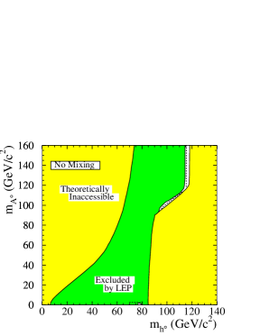
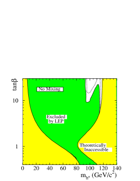
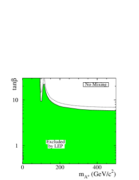
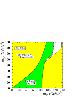
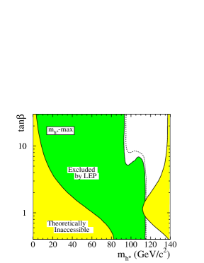
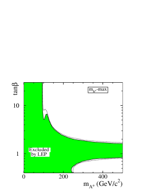
Figure 6: MSSM: limits in the no-mixing and maximum h-mass benchmark scenarios with $m_{\rm t}=179.3$ GeV.

3.2 Three-Neutral-Higgs-Boson Hypothesis and a MSSM Parameter Scan

The hypothesis of three-neutral-Higgs-boson production, via hZ, HZ and hA is compatible with the data excess seen in Fig. 7. For the reported MSSM parameters [6] reduced hZ production near 100 GeV and HZ production near 115 GeV is compatible with the data (left plot). For $m_{\rm h}\approx m_{\rm A}$, hA production is also compatible with the data (center plot). The parameters have been obtained from a general MSSM parameter scan. The overall agreement of data and background is shown in the right plot.

\includegraphics[scale={0.24}]{fig7.eps}

\includegraphics[scale={0.35}]{lepdiagclb.eps}

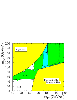
Figure 7: MSSM. Left: small data excess at 99 GeV and 116 GeV in hZ/HZ searches. Center: small data excess at $m_{\rm h}+m_{\rm A}=187$ GeV in hA searches. Right: contours of $1-CL_{\rm b}$ for the maximum h-mass benchmark scenario. $1-CL_{\rm b}$ expresses the incompatibility of the observation with the background-only hypothesis.

3.3 A General MSSM Parameter Scan

Mass limits from a general MSSM parameter scan are shown in Fig. 8 (left plot). After the inclusion of searches for invisible Higgs boson decays, mass limits are only slightly reduced compared to the benchmark results.

3.4 Large $\tan\beta$ Scenario

For large values of $\tan\beta$, MSSM parameter regions exist, where hA production is inaccessible kinematically and hZ production is suppressed by small $\sin(\beta-\alpha)$ values, thus HZ production is dominant. The importance of the HZ contribution is shown in Fig. 8 (center plot) where the mass region between 96 and 107 GeV is excluded from the non-observation of HZ production.

\includegraphics[scale={0.26}]{delphi_mh_ma.eps}

\includegraphics[width=145.68143pt,clip]{259_fig5b.eps}

\includegraphics[width=136.5746pt,bbllx=27pt,bblly=2pt,bburx=258pt,bbury=238pt,clip={}]{o_fig16new.eps}

Figure 8: MSSM. Left: mass limits from a general MSSM parameter scan. Center: excluded mass region for large $\tan\beta$ from h and H searches. Right: much reduced $\tan\beta$ limits due to the larger top-quark mass. The overlap of the shaded regions is reduced for larger top-quark masses.

3.5 Large Effect from Increased Top-Quark Mass

An increased top-quark mass of $178.0\pm 4.3$ GeV has been reported [5]. This mass is about 4 GeV larger compared to the previous value. This larger top-quark mass has an important effect of the Higgs boson search, as a larger top-quark mass results in a larger maximum for the Higgs boson mass. Therefore, in particular the previous limits on $\tan\beta$ are reduced as illustrated in Fig. 8 (right plot).

4 CP-Violating Models

Instead of h, H and A, the Higgs bosons are named $\rm H_{1},H_{2}$ and $\rm H_{3}$. In general, CP-mixing reduces the MSSM mass limits significantly [7]. Combined LEP limits for $m_{\rm t}=179.3$ GeV are shown in Fig. 9.

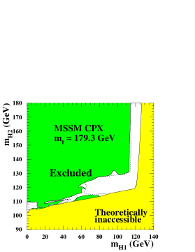
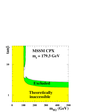
Figure 9: CP-violation models. Limits for full CP-mixing with $m_{\rm t}=179.3$ GeV.

5 Invisible Higgs Boson Decays

No indication of invisibly-decaying Higgs bosons is observed. Figure 10 shows mass limits for SM and invisible Higgs boson decays combined. The results are also interpreted in a Majoron model with an extra complex singlet, $\rm H/S\mbox{$\rightarrow$}JJ$, where J escapes undetected. In addition, mass limits are shown in the MSSM for $\rm h\to\tilde{\chi}^{0}_{1}\tilde{\chi}^{0}_{1}$.

\includegraphics[scale={0.34}]{d_inv_br_hmass.eps}

\includegraphics[scale={0.26}]{d_inv_majoron.eps}

\includegraphics[scale={0.26}]{d_inv_tbmh.eps}

Figure 10: Left: mass limits for SM and invisible Higgs boson decays combined. Center: mass limits in Majoron models with an extra complex singlet, $\rm H/S\mbox{$\rightarrow$}JJ$, where J escapes undetected. $\sin\theta$ is the H/S mixing angle. Right: mass limits in the MSSM for $\rm h\to\tilde{\chi}^{0}_{1}\tilde{\chi}^{0}_{1}$.

6 Neutral Higgs Bosons in the General Two-Doublet Higgs Model

Figures 11 and 12 show mass limits from flavor-independent and dedicated searches for hA production, and from a parameter scan. The scan combines searches with b-tagging and flavor-independent searches.

\includegraphics[scale={0.36}]{d_fblind_fig11.eps}

\includegraphics[scale={0.24}]{d_excludall.eps}

\includegraphics[scale={0.27}]{opal_2dhm.eps}

Figure 11: Two-doublet Higgs model. Left: Flavor-independent limits. $C^{2}$ is the reduction factor on the maximum production cross section. Center: Limits from dedicated searches for hA production. Right: mass limits from a general parameter scan in the two-doublet Higgs model.

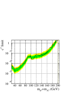
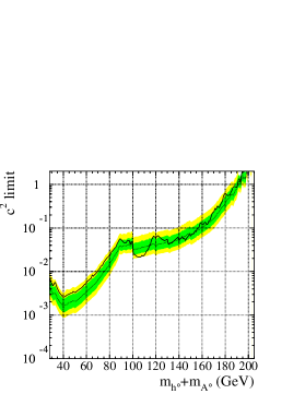
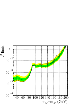
Figure 12: Upper bound on the scale factor $C^{2}$, assuming $m_{\rm h}\approx m_{\rm A}$ Left: typical branching ratios. Center: decay exclusively into b-quark pairs. Right: one decay into a b-quark pair and the other into a $\tau$-lepton pair.

7 Yukawa Higgs Boson Processes $\rm b\bar{b}h$ and $\rm b\bar{b}A$

Figure 13 shows mass limits from searches for the Yukawa processes $\rm e^{+}e^{-}\rightarrow b\bar{b}\rightarrow b\bar{b}h,~{}b\bar{b}A$.

\includegraphics[scale={0.53}]{d_h_4b.eps}

\includegraphics[scale={0.53}]{d_a_4b.eps}

\includegraphics[scale={0.53}]{d_h_bbtt.eps}

\includegraphics[scale={0.53}]{d_a_bbtt.eps}

Figure 13: Observed (solid line) and expected (dotted line) mass limits from searches for the Yukawa processes $\rm e^{+}e^{-}\rightarrow b\bar{b}\rightarrow b\bar{b}h,~{}b\bar{b}A$. The $C$ factors include vertex enhancement factors and decay branching fractions. The 1$\sigma$ and 2$\sigma$ error bands on the expected limit for background are indicated.

8 Singly-Charged Higgs Bosons

Figure 14 shows mass limits from searches for $\rm\mbox{$\mathrm{e}^{+}\mathrm{e}^{-}$}\mbox{$\rightarrow$}H^{+}H^{-}\mbox{$\rightarrow$}c\bar{s}\bar{c}s,~{}cs\tau\nu,~{}\tau^{+}\nu\tau^{-}\bar{\nu}$. The decay $\rm H^{\pm}\mbox{$\rightarrow$}W^{\pm}A$ could be dominant and limits from dedicated searches are set.

\includegraphics[scale={0.3}]{lep_hphm_lim.eps}

\includegraphics[scale={0.27}]{charged-branching-ratios-color.eps}

\includegraphics[scale={0.27}]{delphi_hwa_limit.eps}

Figure 14: Left: excluded mass region (shaded area) from searches for $\rm\mbox{$\mathrm{e}^{+}\mathrm{e}^{-}$}\mbox{$\rightarrow$}H^{+}H^{-}\mbox{$\rightarrow$}c\bar{s}\bar{c}s,$ $\rm cs\tau\nu$ and $\rm\tau^{+}\nu\tau^{-}\bar{\nu}$. The thin line shows the expected limit. Center: $\rm H^{\pm}\mbox{$\rightarrow$}W^{\pm}A$ decays could be dominant for light A boson masses. Right: excluded mass region (shaded area) from searches for this process.

9 Doubly-Charged Higgs Bosons

The process $\rm\mbox{$\mathrm{e}^{+}\mathrm{e}^{-}$}\mbox{$\rightarrow$}H^{++}H^{--}\mbox{$\rightarrow$}\tau^{+}\tau^{+}\tau^{-}\tau^{-}$ can lead to decays at the primary interaction point ($h_{\tau\tau}\geq 10^{-7}$) or a secondary vertex, or to stable massive particle signatures. Figure 15 shows limits on the production cross section and constraints by the forward-backward asymmetry of the process $\mathrm{e}^{+}\mathrm{e}^{-}$$\rightarrow$$\mathrm{e}^{+}\mathrm{e}^{-}$. New results from the Tevatron extend the LEP limits [8, 9].

\includegraphics[scale={0.28}]{opal_doubly349_fig4.eps}

\includegraphics[scale={0.36}]{delphi-doubly-charged-xslim-1.eps}

\includegraphics[width=136.5746pt]{l3_hpp_fig6.eps}

Figure 15: Left and center: limits on the $\rm\mbox{$\mathrm{e}^{+}\mathrm{e}^{-}$}\mbox{$\rightarrow$}H^{++}H^{--}$ production cross section as a function of the doubly-charged Higgs boson mass. The 1$\sigma$ and 2$\sigma$ error bands on the expected limit for background are indicated (shaded areas). Right: $\rm H^{--}$ limits from $\mathrm{e}^{+}\mathrm{e}^{-}$$\rightarrow$$\mathrm{e}^{+}\mathrm{e}^{-}$ forward-backward asymmetry.

10 Fermiophobic Higgs Boson Decays: $\rm h\mbox{$\rightarrow$}$ WW, ZZ, $\gamma\gamma$

If Higgs boson decays into fermions are suppressed, $\rm h\mbox{$\rightarrow$}$ WW, ZZ, $\gamma\gamma$ decays could be dominant. Mass limits from dedicated searches are shown in Fig. 16.

\includegraphics[scale={0.25}]{l3_fermio_fig6.eps}

\includegraphics[scale={0.26}]{lep_fermio_fig5.eps}

Figure 16: Left: mass limits from $\rm h\mbox{$\rightarrow$}$ WW, ZZ, $\gamma\gamma$ searches. Right: mass limits from $\rm h\mbox{$\rightarrow$}\gamma\gamma$ combined LEP results.

11 Uniform and Stealthy Higgs Boson Scenarios

The recoiling mass of the Z boson in the reaction $\rm e^{+}e^{-}\to HZ$ allows to search for the Higgs boson independent of the Higgs boson decay mode. No indication of a Higgs boson signal has been observed as shown in Fig. 17. Mass limits are shown in the uniform Higgs boson model, where many uniform Higgs boson states exist in the range between $m_{\rm A}$ and $m_{\rm B}$. Another result from the recoiling mass spectrum is shown, where a stealthy Higgs boson has a large decay width owing to extra Higgs boson singlets in the model. The decay width depends on the parameter $\omega$.

\includegraphics[width=455.24408pt]{pr355_08a.eps}\includegraphics[width=455.24408pt]{pr355_08b.eps}

\includegraphics[width=227.62204pt]{pr355_12new.ps}\includegraphics[width=223.0721pt]{pr355_14.eps}

Figure 17: Left: recoiling mass spectrum of $\rm Z\to e^{+}e^{-}$ and $\rm Z\to\mu^{+}\mu^{-}$. Center: excluded mass range in the uniform Higgs model. Right: mass limits in the stealthy Higgs model.

12 LEP Summary

Immense progress has been made over a period of about 15 years in searches for Higgs bosons and much knowledge has been gained in preparation for new searches. No signal has been observed and various stringent limits are set as summarized in Table 1.

Table 1: Summary of Higgs boson mass limits at 95% CL. ‘LEP’ indicates a combination of the results from ALEPH, DELPHI, L3 and OPAL. If results from the experiments are not (yet) combined, examples which represent the different research areas from individual experiments are given.

Search	Experiment	Limit
Standard Model	LEP	$m^{\rm SM}_{\rm H}>114.4$ GeV
Reduced rate and SM decay		$\xi^{2}>0.05:$ $m_{\rm H}>85$ GeV
		$\xi^{2}>0.3:$ $m_{\rm H}>110$ GeV
Reduced rate and $\rm b\bar{b}$ decay		$\xi^{2}>0.04:$ $m_{\rm H}>80$ GeV
		$\xi^{2}>0.25:$ $m_{\rm H}>110$ GeV
Reduced rate and $\tau^{+}\tau^{-}$ decay		$\xi^{2}>0.2:$ $m_{\rm H}>113$ GeV
Reduced rate and hadronic decay		$\xi^{2}=1:$ $m_{\rm H}>112.9$ GeV
		$\xi^{2}>0.3:$ $m_{\rm H}>97$ GeV
	ALEPH	$\xi^{2}>0.04:$ $m_{\rm H}\approx 90$ GeV
Anomalous couplings	L3	$d,~{}{d_{\rm B}},~{}{\Delta g_{1}^{{\mathrm{Z}}}},~{}{\Delta\kappa_{\gamma}}$ exclusions
MSSM (no scalar top mixing)	LEP	almost entirely excluded
General MSSM scan	DELPHI	$m_{\rm h}>87$ GeV, $m_{\rm A}>90$ GeV
Larger top-quark mass	LEP	strongly reduced $\tan\beta$ limits
CP-violating models	LEP	strongly reduced mass limits
Visible/invisible Higgs decays	DELPHI	$m_{\rm H}>111.8$ GeV
Majoron model (max. mixing)		$m_{\rm H,S}>112.1$ GeV
Two-doublet Higgs model	DELPHI	$\rm hA\mbox{$\rightarrow$}b\bar{b}b\bar{b}:$ $m_{\rm h}+m_{\rm A}>150$ GeV
(for $\sigma_{\rm max}$)		$\tau^{+}\tau^{-}\tau^{+}\tau^{-}:$ $m_{\rm h}+m_{\rm A}>160$ GeV
		$\rm(AA)A\mbox{$\rightarrow$}6b:$ $m_{\rm h}+m_{\rm A}>150$ GeV
		$\rm(AA)Z\mbox{$\rightarrow$}4b~{}Z:$ $m_{\rm h}>90$ GeV
		$\rm hA\mbox{$\rightarrow$}q\bar{q}q\bar{q}:$ $m_{\rm h}+m_{\rm A}>110$ GeV
Two-doublet model scan	OPAL	$\tan\beta>1:$ $m_{\rm h}\approx m_{\rm A}>85$ GeV
Yukawa process	DELPHI	$C>40:$ $m_{\rm h,A}>40$ GeV
Singly-charged Higgs bosons	LEP	$m_{\rm H^{\pm}}>78.6$ GeV
$\rm W^{\pm}A$ decay mode	DELPHI	$m_{\rm H^{\pm}}>76.7$ GeV
Doubly-charged Higgs bosons	DELPHI/OPAL	$m_{\rm H^{++}}>99$ GeV
$\mathrm{e}^{+}\mathrm{e}^{-}$$\rightarrow$$\mathrm{e}^{+}\mathrm{e}^{-}$	L3	$h_{\rm ee}>0.5:$ $m_{\rm H^{++}}>700$ GeV
Fermiophobic $\rm H\mbox{$\rightarrow$}WW,ZZ,\gamma\gamma$	L3	$m_{\rm H}>108.3$ GeV
$\rm H\mbox{$\rightarrow$}\gamma\gamma$	LEP	$m_{\rm H}>109.7$ GeV
Uniform and stealthy scenarios	OPAL	depending on model parameters

13 International Linear Collider (ILC)

The next generation $\rm e^{+}e^{-}$ collider will be a linear collider. In summer 2004 as a major step forward in the ILC programme a world-wide agreement has been reached that the ILC will operate with the cold technology (superconducting cavities). Since the TESLA Technical Design Report (TDR) [10], the physics programme of an electron-positron linear collider (LC) has been further developed and a wide consensus has been reached on the physics case and the need for a high luminosity LC with center-of-mass energy up to about 1 TeV as the next worldwide high-energy physics project. Recent milestones were set with the Snowmass Study [11] and the international workshops on LC in Korea [12] and Paris [4].

The study of the Higgs boson properties represents a significant part of this physics programme. A linear collider of at least 500 GeV and a total luminosity of at least 1000 fb^-1 has much potential for studying Higgs bosons and understanding the electroweak symmetry breaking and mass generation.

The SM physics is addressed and it is discussed how precisely a future LC can determine the Higgs boson production mechanism. Indirect and direct branching ratio measurements are reviewed. Then the characterization of the Higgs boson potential, which will contribute to establishing the underlying mechanism of mass generation, is addressed. Higgs bosons could also be produced via Higgs-strahlung off top quarks. In the general two Higgs doublet model (2HDM) charged Higgs bosons are prominent. Various methods to determine the ratio of the vacuum expectation values of the two doublets, $\tan\beta$, are discussed. In the framework of the Minimal Supersymmetric extension of the SM (MSSM) or beyond, invisibly decaying Higgs bosons could be produced and their properties measured. It has recently been emphasized that the LC collider precision is essential in the scenario of the decoupling limit (MSSM$\rightarrow$SM) [13]. Furthermore, the measurement of the Higgs boson parity is discussed as well as important possibilities to distinguish Higgs boson models. For several LC studies the relation to the LHC potential is addressed. Future LC Higgs studies will concentrate on more detailed detector simulations reflecting the progress in detector technologies, the second phase of a LC with higher center-of-mass energies, and new theoretical developments, such as extra dimensions.

14 Standard Model Physics

14.1 Higgs boson production mechanism

The expected SM Higgs production rate has a very large significance over the background ($\sigma\equiv N_{\rm sig}/\sqrt{N_{\rm bg}}$). More than $100\sigma$ is obtainable in the $\rm H\rightarrow b\bar{b}$ decay channel. For heavier Higgs bosons, the WW decay mode takes over. In relation to the LHC, a LC has a much larger sensitivity in the lower mass range, while the LHC can probe heavier Higgs bosons. At about 115 GeV mass, the LEP sensitivity reduces from about $4\sigma$ to $2\sigma$. Figure 18 (left plot) shows the SM Higgs boson detection significance.

\includegraphics[scale={0.26}]{smmass_new4.eps}

\includegraphics[scale={0.26}]{xsec.eps}

\includegraphics[scale={0.7},bbllx=284pt,bblly=479pt,bburx=515pt,bbury=631pt,clip={}]{nlchzfusion.eps}

Figure 18: Left: SM Higgs boson signal significance. Center: expected production cross sections (dashed lines) and simulated experimental sensitivities (solid lines). Right: expected missing mass distributions for Higgs-strahlung and WW fusion. Their sum is shown in comparison with simulated data.

The sensitivity to the general production cross section has been studied. The expected SM production cross section is much larger than the $5\sigma$ sensitivity to the cross section over a wide mass range. For lower masses the Higgs boson decay mode into a pair of b-quarks gives the largest sensitivity. Figure 18 (center plot) shows the cross section sensitivity for any Higgs boson decay mode, where the Higgs boson mass is reconstructed as the recoiling mass to the Z decay products. Even for models beyond the SM, the sensitivity to the cross section is much better than the expected minimal production cross section.

The Higgs boson will be produced via Higgs-strahlung and WW fusion by the two processes

$$\rm e^{+}e^{-}\rightarrow HZ\rightarrow H\nu\bar{\nu}\rightarrow b\bar{b}\nu\bar{\nu}~{}~{}~{}and$$

$$\rm e^{+}e^{-}\rightarrow WW\nu\bar{\nu}\rightarrow\nu\bar{\nu}H\rightarrow\nu\bar{\nu}b\bar{b}.$$

These production mechanisms can be distinguished by fitting the missing mass distribution as shown in Fig. 18 (right plot). Higgs-strahlung gives a shape like the dashed line, while Higgs boson fusion is represented by the dotted line. Their sum is given by the solid line and the simulated data is shown with error bars.

14.2 Indirect and direct branching ratio measurements

A LC will perform very high precision measurements of the Higgs boson branching fractions. The underlying production process is the Higgs-strahlung,

$$\rm e^{+}e^{-}\rightarrow HZ\rightarrow H\ell^{+}\ell^{-},$$

where the associated Z boson decays into a lepton pair. Two methods are discussed to determine the Higgs boson branching ratio.

In the indirect method, the inclusive production cross section as the product of the Higgs boson production cross section and the branching fraction of the Z into leptons is determined:

$$\sigma_{\rm inc}=\sigma_{\rm HZ}BR(\rm Z\rightarrow\ell^{+}\ell^{-}).$$

This measurement is independent of the Higgs boson decay mode. The mass recoiling to the lepton pair corresponds to the Higgs boson mass. An individual Higgs boson decay cross section is measured, which is the product of the Higgs boson production cross section and the Higgs and Z boson decay branching fractions:

$$\sigma({\rm X})=\sigma_{\rm HZ}BR({\rm Z\rightarrow Y})BR({\rm H\rightarrow X}).$$

By taking the ratio of both cross sections the Higgs branching ratio can be determined, since the LEP experiments measured the Z decay branching fractions with high precision.

The Higgs boson branching ratios can also be determined directly from the HZ($\rm Z\rightarrow\ell^{+}\ell^{-}$) event sample. The Higgs boson mass is reconstructed as the recoiling mass of the lepton pair:

$$m_{\rm H}=m_{\ell^{+}\ell^{-}}^{\rm recoil}.$$

The simulation was performed for $\sqrt{s}=360$ GeV and ${\cal L}=500$ fb^-1. Figure 19 (left plot) shows this event sample which is enriched with Higgs bosons by the indicated cuts. The expected signal distribution is given with error bars and the expected background as a histogram. In this event sample individual Higgs boson decay modes are selected. The resulting precision on the Higgs boson decay branching ratios as well as a preliminary combination of both methods are listed in Table 2. For the c-quark decay mode, recently a larger uncertainty of 12.1% was reported [14]. The variation of the branching ratio precision as a function of the Higgs boson mass is shown as well in Table 2 [15].

Table 2: Left: expected precision on branching ratios (in %) for a 120 GeV Higgs boson from the direct method (d) and a preliminary combination (c) with the indirect method. Right: variation of the $BR({\rm H\to b\bar{b}})$ precision (in %) as a function of the Higgs boson mass.

Decay	SM $BR$	$\Delta BR_{\rm d}/BR_{\rm d}$	$\Delta BR_{\rm c}/BR_{\rm c}$
bb	68	1.9	1.5
$\tau\tau$	6.9	7.1	4.1
cc	3.1	8.1	5.8
gluons	7.0	4.8	3.6
$\gamma\gamma$	0.22	35	21
WW⋆	13	3.6	2.7

$m_{\rm H}$ (GeV)	120	140	160	160
$\Delta BR_{\rm b}/BR_{\rm b}$	1.6	1.8	2.0	9.0

In relation to the LHC, a LC will achieve a much higher precision and will cover all decay modes. This would also allow precision testing of the fundamental relation between the Yukawa coupling and the Higgs boson mass:

$$g_{\rm Hff}\propto m_{\rm f}.\vspace*{-3mm}$$

\includegraphics[scale={0.26}]{fig2_br.eps}

\includegraphics[scale={0.5}]{h240.eps}

\includegraphics[scale={0.28}]{0102342.fig3.ps}

Figure 19: Left: simulated events for a direct determination of the Higgs boson decay branching ratios. Center: mass and width determination. Right: comparison of different methods to determine the Higgs boson mass.

14.3 Mass and width determination

Further properties of the Higgs boson, like its mass and decay width, can be determined with high precision. A study of a 240 GeV SM Higgs boson in the reactions

$$\rm e^{+}e^{-}\rightarrow HZ\rightarrow WWZ~{}~{}~{}and$$

$$\rm e^{+}e^{-}\rightarrow HZ\rightarrow ZZZ$$

has been performed. A very clear signal with only a few background events is expected. Figure 19 (center plot) shows the expected signal and background mass distribution. The fit (center plot) of the reconstructed mass peak leads to a mass resolution of 0.08% and an 11% error on the total decay width. Figure 19 (right plot) shows results from a CMS study (curve 1) where the Higgs boson decays into a pair of Z bosons, which subsequently decay into muon pairs. The sensitivity reduction near 160 GeV is due to dominant decays into W pairs. The curves 2 and 3 show extrapolated results according to the cross section and branching ratio expectations for a LC operation at 350 and 500 GeV. In the low mass region indirect methods can be applied (curve 4) and for very low masses, the LHC has high sensitivity in the photon decay mode.

High precision $\Delta E/E_{\rm beam}<10^{-4}$ is needed to achieve a mass precision of $m_{\rm H}=120.00\pm 0.04$ GeV [16]. It has been pointed out [17] that the expected experimental precision $\Delta m^{\rm exp}_{\rm h}\approx 0.05$ GeV is difficult to match in the theoretical prediction $\Delta m^{\rm th}_{\rm current}\approx 3$ GeV and $\Delta m^{\rm th}_{\rm future}\approx 0.5$ GeV.

The tagging of b- and c-quarks are crucial for the Higgs boson studies as the Higgs boson decays predominantly into heavy quarks. Figure 20 (left plot) shows the efficiency versus purity for a CCD vertex detector simulation [18]. With this vertex detector the process $\rm HA\to b\bar{b}b\bar{b}$ at $\sqrt{s}=800$ GeV has been studied and Fig. 20 (right plot) shows that a precision of $\Delta m_{\rm H}\approx\Delta m_{\rm A}\approx 0.45$ GeV can be achieved [19].

\includegraphics[scale={0.6}]{tagging.eps}

\includegraphics[scale={0.2}]{mass300250.eps}

Figure 20: Left: c- and b-tagging efficiency versus purity for the LCFI vertex detector. Right: reconstructed mass difference for the reaction $\rm HA\to b\bar{b}b\bar{b}$ at $\sqrt{s}=800$ GeV with Higgs boson masses of 250 and 300 GeV.

14.4 Characterization of the Higgs boson potential

A LC will be able to measure fundamental properties of the Higgs boson potential. The Higgs boson can decay into a pair of Higgs bosons:

$$\rm e^{+}e^{-}\rightarrow HZ\rightarrow HHZ.$$

Figure 21 illustrates this Higgs boson production reaction.

\includegraphics[scale={0.26}]{marcofig2.eps}\includegraphics[scale={0.26}]{marcofig4.eps}

Figure 21: Left: Higgs boson self-coupling reaction. Center: reconstructed invariant mass of the HH pairs. Right: reconstructed angle between the H and HH directions.

The self-coupling interaction can probe the shape of the Higgs boson potential through the relation

$$g_{\rm HHH}=3m_{\rm H}^{2}/2v,$$

where $v=246$ GeV. A sensitivity of $\Delta g/g=29$% was obtained for $m_{\rm H}=120$ GeV, $\sqrt{s}=800$ GeV and ${\cal L}=1000$ fb^-1. Figure 21 shows the precision on the Higgs boson self-coupling where the lines indicate $g_{\rm HHH}/g_{\rm HHH}^{\rm SM}=1.25,~{}1.00,~{}0.75,~{}0.50$. Higher sensitivity of $\Delta g/g=7$% could be reached for a LC with $\sqrt{s}=3$ TeV and ${\cal L}=5000$ fb^-1 as shown in Fig. 21.

14.5 Higgs-strahlung from top quarks

Owing to the strong coupling of Higgs bosons to top quarks, the radiation of Higgs boson off top quarks is a possible production mechanism. The decay modes involving a pair of b quarks and W bosons were studied in the reactions

$$\rm e^{+}e^{-}\rightarrow t\bar{t}H\rightarrow t\bar{t}b\bar{b}~{}~{}~{}and$$

$$\rm e^{+}e^{-}\rightarrow t\bar{t}H\rightarrow t\bar{t}WW.$$

A challenge is the precision determination of the background to a level of 5% uncertainty, leading to

$$\Delta g_{\rm ttH}/g_{\rm ttH}=7.5\%~{}{\rm to}~{}20\%.$$

Figure 22 (left plot) shows the resulting precision for the $\rm b\bar{b}$ and WW decay modes, as well as their statistical combination as a function of the SM Higgs boson mass. A similar sensitivity was recently confirmed [20]. In addition, a previous study at 120 GeV with slightly higher sensitivity is indicated. The reaction $\rm H\rightarrow ZZ$ is currently under study [21].

15 Beyond the Standard Model

15.1 Charged Higgs bosons

The discovery of charged Higgs bosons would immediately prove that physics beyond the SM exists. The reaction

$$\rm e^{+}e^{-}\rightarrow Z\rightarrow H^{+}H^{-}\rightarrow t\bar{b}\bar{t}b$$

can be observed at a LC and recent high-luminosity simulations show that the production cross section times branching ratio can be measured very precisely:

$$\Delta(\sigma BR({\rm H^{+}\rightarrow t\bar{b}}))/\sigma BR({\rm H^{+}\rightarrow t\bar{b}})=8.8\%$$

for $m_{\rm H^{\pm}}=300$ GeV, $\sqrt{s}=800$ GeV and ${\cal L}=1000$ fb^-1. A detailed reconstruction of the entire decay chain, as illustrated in Fig. 22 (center plot), is possible. Figure 22 (right plot) shows also a clear expected charged Higgs boson signal and small background.

\includegraphics[scale={0.22}]{yukawacoupling_asopczak.eps}

\includegraphics[scale={0.55}]{feyn2.ps}

\includegraphics[scale={0.26}]{arifig3.eps}

Figure 22: Left: expected precision on the Yukawa coupling $g_{\rm ttH}$. Center: charged Higgs boson production and decay. Right: expected charged Higgs boson signal and background.

15.2 Determination of $\tan\beta$

The ratio of the vacuum expectation values $\tan\beta$ can be measured with several methods. The pseudoscalar Higgs boson, A, could be produced via radiation off a pair of b-quarks:

$$\rm e^{+}e^{-}\rightarrow b\bar{b}\rightarrow b\bar{b}A\rightarrow b\bar{b}b\bar{b}.$$

The $\rm b\bar{b}A$ coupling is proportional to $\tan\beta$ and thus the expected production rate is proportional to $\tan^{2}\beta$. A precision better than 10% can be achieved for a Higgs boson mass of 100 GeV and large $\tan\beta$ values. The sensitivity decreases with increasing Higgs boson masses and decreasing $\tan\beta$ values as shown in Fig. 23 (left plot). This study assumes a luminosity of 2000 fb^-1, corresponding to several years of data taking. There are further methods to determine $\tan\beta$:

• The $\rm b\bar{b}\bar{b}b$ rate from the pair-production of the heavier scalar in association with the pseudoscalar Higgs boson,

  $$\rm e^{+}e^{-}\rightarrow HA\rightarrow b\bar{b}b\bar{b},$$

  can be exploited. While the HA production rate is almost independent of $\tan\beta$ the sensitivity is achieved owing to the variation of the decay branching ratios with $\tan\beta$.

• The value of $\tan\beta$ can also be determined from the H and A decay widths, which can be obtained from the previously described reaction.

• The pair-production rate and total decay width of charged Higgs bosons can contribute to the determination of $\tan\beta$. Charged Higgs boson production can also be used at the LHC to measure $\tan\beta$.

\includegraphics[scale={0.21}]{fig03.eps}

\includegraphics[scale={0.26},angle={90}]{fig04.eps}

\includegraphics[scale={0.31}]{br_andre.eps}

Figure 23: Left: 2HDM $\tan\beta$ determination. Center: MSSM $\tan\beta$ determination. Right: expected precision on the invisible Higgs boson branching fraction. The dots represent the indirect method.

The results from the methods involving the neutral Higgs bosons are summarized in Fig. 23 (center plot) for the MSSM. As the H and A decay rates depend on the MSSM parameters, two cases are considered. In case (I) heavy Supersymmetric particles are expected, while in case (II) the Higgs bosons could decay into light Supersymmetric particles.

15.3 Invisible Higgs boson decays

Among other possibilities, invisible Higgs boson decays could occur from the reaction involving neutralinos:

$$\rm e^{+}e^{-}\rightarrow ZH\rightarrow Z\tilde{\chi}^{0}\tilde{\chi}^{0}.$$

In this case the Higgs boson mass can be reconstructed from the recoiling mass of the visible decay products:

$$m_{\rm H}=m_{\rm Z}^{\rm recoil}.$$

At LEP all Z decay modes involving charged fermions contributed to the search, while in a recent LC study so far only the hadronic decay mode $\rm Z\rightarrow q\bar{q}$ has been investigated. This study for $\sqrt{s}=350$ GeV and ${\cal L}=500$ fb^-1 gives higher sensitivity compared to indirect methods ($1-$ sum of visible H decay modes). For Higgs boson branching ratios $BR_{\rm i}$ into invisible decay products larger than 20% and a SM Higgs boson production rate,

$$\Delta BR_{\rm i}/BR_{\rm i}<4\%$$

can be achieved. Figure 23 (right plot) shows the resulting sensitivities as a function of the branching ratio into invisible decays.

15.4 Higgs boson parity

After the discovery of one or several Higgs bosons, it would be very important to determine the parity of the Higgs bosons and distinguish a CP-even H boson from a CP-odd A boson. This could be achieved by investigating the Higgs boson decay properties into $\tau$-leptons. The subsequent decay of the $\tau$’s into $\rho$’s and pions through the reaction

$$\rm H/A\rightarrow\tau^{+}\tau^{-}\rightarrow\rho^{+}\bar{\nu}_{\tau}\rho^{-}\nu_{\tau}\rightarrow\pi^{+}\pi^{0}\bar{\nu}_{\tau}\pi^{-}\pi^{0}\nu_{\tau}$$

is studied.

The $\rho^{+}\rho^{-}$ acoplanarity angle is defined by the planes of the pions in the rest frame of the $\rho$’s as illustrated in Fig. 24 (left plot). The acoplanarity angle distribution clearly distinguishes the different parity states. Figure 24 (center plot) shows the acoplanarity angle before detector effects are included, and Fig. 24 (right plot) after a preliminary detector simulation. The thick line is the expectation for scalar Higgs bosons and the thin line for pseudoscalar Higgs bosons.

\includegraphics[scale={0.6}]{rho_acop_fig.ps}

\includegraphics[scale={0.35}]{0204292.fig1.ps}

\includegraphics[scale={0.35}]{0204292.fig3.ps}

Figure 24: Left: acoplanarity angle definition. Center: Higgs boson parity determination before detector simulation. Right: Higgs boson parity determination after a preliminary detector simulation.

15.5 Distinction of Higgs boson models

The distinction of Higgs boson models is very important and could be based on precision branching ratio measurements. The ratio of the Higgs boson decay rates into b-quarks and $\tau$-leptons is defined by

$$R\equiv BR({\rm H/A\rightarrow b\bar{b})}/BR({\rm H/A\rightarrow\tau^{+}\tau^{-}}).$$

The normalized value of $R$ to the SM expectation can be used to distinguish a general 2HDM from the MSSM. Large deviations from $R=1$ are expected in the MSSM for several MSSM parameter combinations as shown in Fig. 25 (left plot). In relation to the LHC, where models can only be distinguished for $\tan\beta>25$, a LC covers the entire $\tan\beta$ range.

\includegraphics[scale={0.3}]{topaper_tb_other.eps}

\includegraphics[scale={0.3}]{lclhc_new3.eps}

Figure 25: Left: distinction of Higgs boson models from precision Higgs boson decay branching ratio determinations. Right: comparison of LHC and LC A mass predictions from precision scalar Higgs boson decay branching ratio determinations.

Important predictions on the pseudoscalar Higgs boson mass can be made from the precision measurements of the scalar Higgs boson branching ratios:

$$BR({\rm H\rightarrow b\bar{b}})/BR({\rm H\rightarrow WW}).$$

A LC obtains a precision normalized to the SM expectation of less than $3.5$%, while the expected precision at the LHC is less than $20$%. For a 400 GeV pseudoscalar Higgs boson A, its mass can be predicted at a LC with an error of about 50 GeV, while at the LHC only a lower mass limit can be set. Figure 25 (right plot) shows the sensitivity on the prediction of the A boson mass at the LHC and a LC for a wide range of A masses.

Beyond the MSSM, the Higgs boson particle spectrum is enriched for example in the framework of the Non-Minimal Supersymmetric extension of the SM (NMSSM) where an extra Higgs boson singlet $\lambda NH_{1}H_{2}$ is present. Such a model could be distinguished from the MSSM by precision measurements of the Higgs boson masses and comparison with the predictions. Moreover, additional light neutral Higgs bosons may be observed and the mass sum rules are modified, leading, for example, to a reduced mass of the charged Higgs boson.

16 Conclusions

At LEP various stringent limits from direct Higgs boson searches are set. Small but intriguing data accesses have been observed. Much knowledge has been gained at LEP in preparation for new searches. After a first discovery and initial precision measurements in some decay modes at the Tevatron or the LHC, already in the first phase of a LC, many Higgs boson decay modes will be measured with very high precision. The precise LC data will allow the determination of the nature of the Higgs sector. Models like the SM, the general 2HDM, the MSSM and the NMSSM will be distinguished for a wide range of parameters. The underlying mechanism of symmetry breaking and mass generation will be tested. Like for the top quark (LEP mass prediction, Tevatron observation), important consistencies of the model can be probed with combined LC and LHC physics. After about 12 years of preparatory studies the LC has a solid case and the high-energy physics community is prepared to answer fundamental questions over the coming decades.

References

- [1] ALEPH, DELPHI, L3 and OPAL Collaborations and the LEP working group for Higgs boson searches, Phys. Lett. B 565 (2003) 61.
- [2] ALEPH, DELPHI, L3 and OPAL Collaborations, contributed papers to the ICHEP’04 Conference, Beijing, and updates.
- [3] A. Sopczak, hep-ph/0209372, Proc. ICHEP’02, Amsterdam, p. 241, and references therein.
- [4] Int. Workshop on LC, Paris, France, April 2004.
- [5] CDF Collaboration, D0 Collaboration, the Tevatron Electroweak Working Group, hep-ex/0404010.
- [6] A. Sopczak, Proc. DPF-2000, hep-ph/0011285; Proc. Topical seminar on the legacy of LEP and SLC, Siena, Nucl. Phys. Proc. Supp. 109 (2002) 271.
- [7] A. Sopczak, hep-ph/0408047, proc. DIS’04, Slovakia, 2004, p. 1017.
- [8] D0 Collaboration, V.M. Abazov, et al., Phys. Rev. Lett. 93 (2004) 141801.
- [9] CDF Collaboration, D. Acosta, et al., Phys. Rev. Lett. 93 (2004) 221802.
- [10] TESLA TDR, DESY (2001).
- [11] American Physical Society study on the future of particle physics, Snowmass, USA, July 2001.
- [12] Int. Workshop on LC, Jeju, Korea, Aug. 2002.
- [13] H. Haber, Int. Workshop on LC, Paris, France, April 2004.
- [14] T. Kuhl, Int. Workshop on LC, Paris, France, April 2004.
- [15] T. Barklow, Int. Workshop on LC, Paris, France, April 2004.
- [16] A. Raspereza, Int. Workshop on LC, Paris, France, April 2004.
- [17] S. Heinemeyer, Int. Workshop on LC, Paris, France, April 2004.
- [18] LCFI Collaboration, C. Damerell etal, Int. Workshop on LC, Paris, France, April 2004.
- [19] K. Desch, T. Klimkovish, T. Kuhl, A. Raspereza, Int. Workshop on LC, Paris, France, April 2004.
- [20] S. Yamashita, Int. Workshop on LC, Paris, France, April 2004.
- [21] A. Gay, A. Besson, M. Winter, Int. Workshop on LC, Paris, France, April 2004.