PITHA 05/01

hep-ph/0501289

31 January 2005

Third-order Coulomb corrections
to the S-wave Green function, energy levels and wave functions at the origin

M. Beneke, Y. Kiyo, K. Schuller

Institut für Theoretische Physik E, RWTH Aachen,
D – 52056 Aachen, Germany

We obtain analytic expressions for the third-order corrections due to the strong interaction Coulomb potential to the $S$-wave Green function, energy levels and wave functions at the origin for arbitrary principal quantum number $n$. Together with the known non-Coulomb correction this results in the complete spectrum of $S$-states up to order $\alpha_{s}^{5}$. The numerical impact of these corrections on the Upsilon spectrum and the top quark pair production cross section near threshold is estimated.

1 Introduction

Several years ago advances in non-relativistic effective theory made it possible to compute quarkonium properties at the next-to-next-to-leading order (NNLO). Since the perturbative approach assumes that the non-relativistic energy scale $E\sim m\alpha_{s}^{2}$ is larger than the strong interaction scale $\Lambda_{\rm QCD}$, these computations apply to the lowest bottomonium states and heavy quark current spectral functions near threshold such as those relevant to top quark pair production. NNLO results have been obtained for matching coefficients [1, 2, 3], energy levels [4, 5, 6, 7], wave functions at the origin [5, 6, 7] and spectral functions [6, 7, 8, 9, 10], principally for the $S$-wave states, which are the most important ones for applications [11].

It was observed that the perturbative corrections are almost always very large. Although the origin of these large corrections can sometimes be understood as being due to mass renormalization [12] or large logarithms, it is currently believed that a complete third (next-to-next-to-next-to-leading/NNNLO) order calculation is necessary to describe accurately even the case of top quark pair production near threshold. That this is a difficult undertaking is reflected by the fact that partial results at NNNLO exist for various quantities [13, 14, 15, 16, 17, 18, 19, 20, 21, 22, 23], but only the $S$-wave ground state energy is currently fully known at third order [24], save for an unknown constant $a_{3}$ in the Coulomb potential. In this paper, we take one further step and compute the NNNLO corrections from the QCD Coulomb potential to the $S$-wave energy levels and wave function at the origin for arbitrary principal quantum number $n$, and to the $S$-wave Green function (spectral function) relevant to top quark pair production. Together with the known non-Coulomb energy level corrections [18, 25] this determines the $S$-wave energy levels completely at third order for any $n$. The correction to the Green function and wave functions at the origin forms part of the complete third-order top quark pair production cross section. Another motivation for first concentrating on the Coulomb corrections is that the Schrödinger equation with the Coulomb potential can be solved numerically, and the result can be compared to the perturbative computation. This is no longer possible once the singular non-Coulomb potentials are included, in which case the perturbative approach is the only option. Comparing the perturbative approximation to the numerical solution allows us to estimate the convergence of the successive approximations.

2 Outline of the calculation

The computation of Coulomb corrections can be phrased in the language of elementary quantum mechanics. We consider the Hamiltonian

$$H=-\frac{{\bf\nabla}^{\,2}}{m}+V(\mbox{\boldmath${r}$}),$$ (1)

where $m$ denotes the heavy quark pole mass, and $V$ the Coulomb potential of the strong force. With

$$V(\mbox{\boldmath${r}$})=\int\frac{d^{3}\mbox{\boldmath${q}$}}{(2\pi)^{3}}\,e^{-i\mbox{\boldmath\footnotesize$q$}\mbox{\boldmath\footnotesize$x$}}\,\tilde{V}(\mbox{\boldmath${q}$}),$$ (2)

the potential reads, up to the fourth order in the expansion in the strong coupling $\alpha_{s}$,

$$\tilde{V}(\mbox{\boldmath${q}$}) = -\frac{4\pi C_{F}\alpha_{s}}{\mbox{\boldmath${q}$}^{2}}+\delta\tilde{V}(\mbox{\boldmath${q}$}),$$ (3)

$$\delta\tilde{V}(\mbox{\boldmath${q}$}) = -\frac{4\pi C_{F}\alpha_{s}}{\mbox{\boldmath${q}$}^{2}}\Bigg{\{}\frac{\alpha_{s}}{4\pi}\bigg{[}a_{1}+\beta_{0}\ln\frac{\mu^{2}}{\mbox{\boldmath${q}$}^{2}}\bigg{]}+\left(\frac{\alpha_{s}}{4\pi}\right)^{\!2}\bigg{[}a_{2}+\Big{(}2a_{1}\beta_{0}+\beta_{1}\Big{)}\ln\frac{\mu^{2}}{\mbox{\boldmath${q}$}^{2}}+\beta_{0}^{2}\ln^{2}\frac{\mu^{2}}{\mbox{\boldmath${q}$}^{2}}\bigg{]}$$ (4)

$$\,+\left(\frac{\alpha_{s}}{4\pi}\right)^{\!3}\bigg{[}a_{3}+8\pi^{2}C_{A}^{3}\ln\frac{\nu^{2}}{\mbox{\boldmath${q}$}^{2}}+\Big{(}3a_{2}\beta_{0}+2a_{1}\beta_{1}+\beta_{2}\Big{)}\ln\frac{\mu^{2}}{\mbox{\boldmath${q}$}^{2}}$$

$$\hskip 54.06006pt+\,\Big{(}3a_{1}\beta_{0}^{2}+\frac{5}{2}\beta_{0}\beta_{1}\Big{)}\ln^{2}\frac{\mu^{2}}{\mbox{\boldmath${q}$}^{2}}+\beta_{0}^{3}\ln^{3}\frac{\mu^{2}}{\mbox{\boldmath${q}$}^{2}}\bigg{]}\Bigg{\}}.$$

Here $\beta_{i}$ are the coefficients of the QCD $\beta$-function in the $\overline{\rm MS}$-scheme, defined with the convention $\partial a_{s}/\partial\ln\mu^{2}=-\sum\beta_{n}a_{s}^{n+2}$, $a_{s}\equiv\alpha_{s}/(4\pi)$ such that $\beta_{0}=11C_{A}/3-4T_{F}n_{f}/3$ [26]. The constants $a_{1}$, $a_{2}$ are given in [3], the $\alpha_{s}^{4}C_{A}^{3}\ln\nu^{2}/\mbox{\boldmath${q}$}^{2}$ term is from [13], while the three-loop constant term $a_{3}$, currently unknown, is estimated to be 6240 ($n_{f}=4$) and 3840 ($n_{f}=5$) [27]. The group theory factors for SU($N_{c}$) gauge theory ($N_{c}=3$ in QCD) are $C_{F}=(N_{c}^{2}-1)/(2N_{c})$, $C_{A}=N_{c}$, $T_{F}=1/2$, and $n_{f}$ denotes the number of quarks whose masses are smaller than $m\alpha_{s}$ and neglected ($n_{f}=4$ for bottom systems, $n_{f}=5$ for top). $\alpha_{s}$ refers to the strong coupling in the $\overline{\rm MS}$ scheme at the renormalization scale $\mu$, while $\nu$ is a scale necessary to define the separation of potential and ultrasoft effects. The dependence on this factorization scale cancels in physical quantities when the ultrasoft correction is included.

When $\delta\tilde{V}(\mbox{\boldmath${q}$})=0$ the spectrum of the Hamiltonian reproduces the well-known Bohr energy levels. This will be our zeroth order approximation. We consider quarkonium systems in which $\alpha_{s}(m\alpha_{s})$ is small, and compute the spectrum in a perturbation expansion in $\alpha_{s}$. Hence, the coefficient of $\alpha_{s}^{n+1}$ in $\delta\tilde{V}(\mbox{\boldmath${q}$})$ is considered a perturbation of the $n$th order, and the third-order result we are aiming at requires up to three insertions of the $\alpha_{s}^{2}$ potential, but only one insertion of the order $\alpha_{s}^{4}$ potential. We shall focus on the $S$-wave Green function

$$G(E)\equiv\langle 0|\hat{G}(E)|0\rangle=\langle 0|\frac{1}{H-E-i\epsilon}|0\rangle,$$ (5)

where $|0\rangle$ denotes a position eigenstate with eigenvalue $\mbox{\boldmath${r}$}=0$, and compute the matrix element of the right-hand side of (omitting the argument $E$ of the Green function)

$$\hat{G} = \hat{G}_{0}-\hat{G}_{0}\delta V_{1}\hat{G}_{0}-\hat{G}_{0}\delta V_{2}\hat{G}_{0}+\hat{G}_{0}\delta V_{1}\hat{G}_{0}\delta V_{1}\hat{G}_{0}$$ (6)

$$-\,\hat{G}_{0}\delta V_{3}\hat{G}_{0}+2\hat{G}_{0}\delta V_{1}\hat{G}_{0}\delta V_{2}\hat{G}_{0}-\hat{G}_{0}\delta V_{1}\hat{G}_{0}\delta V_{1}\hat{G}_{0}\delta V_{1}\hat{G}_{0}.$$

$G_{0}(E)$ denotes the zeroth-order Green function, and $\delta V_{n}$ the $n$th order perturbation potential. The Green function $G(E)$ has single poles at the exact $S$-wave energy levels $E=E_{n}$, such that

$$G(E)\stackrel{{\scriptstyle E\to E_{n}}}{{=}}\frac{|\psi_{n}(0)|^{2}}{E_{n}-E-i\epsilon}.$$ (7)

Inserting

$$E_{n} = E_{n}^{(0)}\left(1+\frac{\alpha_{s}}{4\pi}e_{1}+\left(\frac{\alpha_{s}}{4\pi}\right)^{\!2}e_{2}+\left(\frac{\alpha_{s}}{4\pi}\right)^{\!3}e_{3}+\ldots\right),$$ (8)

$$\ |\psi_{n}(0)|^{2} = |\psi_{n}^{(0)}(0)|^{2}\left(1+\frac{\alpha_{s}}{4\pi}f_{1}+\left(\frac{\alpha_{s}}{4\pi}\right)^{\!2}f_{2}+\left(\frac{\alpha_{s}}{4\pi}\right)^{\!3}f_{3}+\ldots\right)$$ (9)

into this equation, we can determine $e_{1,2,3}$ and $f_{1,2,3}$ by comparing the expansion of (7) in $\alpha_{s}$ with (6) near $E=E_{n}$. We recall that $E_{n}^{(0)}=-m(\alpha_{s}C_{F})^{2}/(4n^{2})$, and $|\psi_{n}^{(0)}(0)|^{2}=(m\alpha_{s}C_{F})^{3}/(8\pi n^{3})$. The details of the calculation are too lengthy to be reproduced here. However, we sketch the computation of the threefold insertion $\langle 0|\hat{G}_{0}\delta V_{1}\hat{G}_{0}\delta V_{1}\hat{G}_{0}\delta V_{1}\hat{G}_{0}|0\rangle$ of $\delta V_{1}$ in the Appendix.

There is an equivalent quantum-field-theoretical description of the calculation, which is the appropriate one in the context of systematic higher-order computations of quarkonium properties [11]. After all the quantum-mechanical description breaks down beyond some accuracy, since (a) the system is sensitive to the short-distance quantum fluctuations, and (b) the restriction to the quark-antiquark sector of the Fock space is inadequate. Systematic calculations therefore start from QCD and obtain effective Lagrangians by systematically integrating out short-distance fluctuations ($\Delta x\sim 1/m$) as well as all massless degrees of freedom down to the ultrasoft energy scale $E\sim m\alpha_{s}^{2}$, which characterizes the size of energy fluctuations in a quarkonium bound state. The result is an effective Lagrangian, in which the potentials appear as matching coefficients [28, 29]. In particular the Coulomb potential is regarded as the matching coefficient of a relevant operator, and differs from the Wilson loop definition beginning at order $\alpha_{s}^{4}$. Consequently, the $\alpha_{s}^{4}\ln\alpha_{s}$ term which appears in the static potential [30] is absent, and replaced by a logarithm of the factorization scale $\nu$ [13] as shown in (4). The computation of Coulomb corrections is based on the Lagrangian

$${\cal L}_{\rm eff} = \psi^{\dagger}(x)\left(i\partial^{0}+\frac{\mbox{\boldmath${\partial}$}^{2}}{2m}\right)\psi(x)+\chi^{\dagger}(x)\left(i\partial^{0}-\frac{\mbox{\boldmath${\partial}$}^{2}}{2m}\right)\chi(x)$$ (10)

$$+\,\int d^{3}\mbox{\boldmath${r}$}\,\left[\psi^{\dagger}\psi\right]\!(x+\mbox{\boldmath${r}$}\,)\,V(\mbox{\boldmath${r}$})\left[\chi^{\dagger}\chi\right]\!(x),$$

where $V(\mbox{\boldmath${r}$})$ is the (colour-singlet) Coulomb potential, and where the non-relativistic two-component field $\psi(x)$ ($\chi(x)$) destroys (creates) a heavy quark (anti-quark). There are other terms in the effective Lagrangian that have to be included for a complete NNNLO calculation. The point we wish to make here is that these are well-understood, and hence there is a well-defined procedure to separate the complete calculation into several simpler parts, of which the calculation of Coulomb corrections is one. An important feature of (10) is that the leading-order Coulomb potential cannot be treated as a perturbation, and must be included in the zeroth order approximation together with the bilinear terms. $\hat{G}_{0}$ is essentially the propagator of this theory. We can also obtain $G(E)$ in (5) directly by computing the two point function

$$N_{c}G(E)=i\int d^{4}x\,e^{iqx}\,\langle\Omega|T([\psi^{\dagger}\chi](x)[\chi^{\dagger}\psi](0)|\Omega\rangle,$$ (11)

with $|\Omega\rangle$ the Fock space vacuum state. This makes it clear that the Green function is closely related to inclusive heavy quark-anti-quark cross sections in $e^{-}e^{+}$ collisions, where the case of the top quark is particularly interesting.

3 Third-order corrections to bound state parameters

In this section we present our result for the third-order correction from the Coulomb potential to the $S$-wave energy levels and wave functions at the origin (squared) for arbitrary principal quantum number $n$. The corrections (notation as in (8,9)) are parameterized as

$$e_{i}=e_{i}^{C}+e_{i}^{nC},$$ (12)

$$f_{i}=f_{i}^{C}+f_{i}^{nC},$$ (13)

where $C$ stands for the correction, when only the Coulomb potential is included in the effective Lagrangian. By definition ‘$nC$’ denotes all the remaining corrections, which originate from additional potentials and an ultrasoft non-potential interaction. Together with the non-Coulomb third-order correction $e_{3}^{nC}$ to energy level [18, 25], we obtain a complete result for the bound state energies to order $m\alpha_{s}^{5}$ for any $n$. For the wave function, however, $f_{3}^{nC}$ is not yet known. We should emphasize that we define $|\psi_{n}(0)|^{2}$ by the residue of the correlation function (11) of non-relativistic currents. The non-Coulomb corrections arise from potentials which cause short-distance singularities, such that $f_{i}^{nC}$ are factorization scheme-dependent quantities. This scheme-dependence is canceled by short-distance coefficients, which we do not discuss here, but which are known to the same order as $f_{i}^{nC}$ is known ($i\leq 2$).

3.1 Energy levels

The energy corrections from the Coulomb potential are organized as follows,

$$e_{1}^{C} = 4\beta_{0}\,L+c_{E,1},$$ (14)

$$e_{2}^{C} = 12\beta_{0}^{2}\,L^{2}+L\,\bigg{(}-8\beta_{0}^{2}+4{\beta_{1}}+6\beta_{0}c_{E,1}\bigg{)}+c_{E,2},$$ (15)

$$e_{3}^{C} = 32\beta_{0}^{3}\,L^{3}+L^{2}\,\bigg{(}-56\beta_{0}^{3}+28\beta_{0}{\beta_{1}}+24\beta_{0}^{2}c_{E,1}\bigg{)}$$ (16)

$$+L\,\bigg{(}16\beta_{0}^{3}-16\beta_{0}{\beta_{1}}+4{\beta_{2}}-12\beta_{0}^{2}c_{E,1}+6{\beta_{1}}c_{E,1}+8\beta_{0}c_{E,2}\bigg{)}$$

$$+c_{E,3}+32\pi^{2}C_{A}^{3}\bigg{[}\ln\left(\frac{n\nu}{mC_{F}\alpha_{s}}\right)+S_{1}(n)\bigg{]},$$

where $L=\ln\left(n\mu/(mC_{F}\alpha_{s})\right)$ and $S_{a}(n)=\sum_{k=1}^{n}1/k^{a}$ is the harmonic sum. For later convenience we introduce the nested harmonic sums

$$S_{a,b}(n)\equiv\sum_{k=1}^{n}\frac{1}{{k}^{a}}\,S_{b}(k),\hskip 28.45274ptS_{a,b,c}(n)\equiv\sum_{k=1}^{n}\frac{1}{k^{a}}\,S_{b,c}(k).$$ (17)

In the following we omit the argument of harmonic sums which is always understood to be the principal quantum number $n$. The coefficients of the logarithmic terms are fixed by the renormalization group in terms of the $\beta$-function and the $c_{E,i}$ from lower orders. The “non-trivial” information is encoded in the constants $c_{E,\,i}$. The first and second order corrections, $c_{E,\,1},c_{E,\,2}$ are known [4, 5, 6, 7]

$$c_{E,\,1} = 2a_{1}+4S_{1}\beta_{0},$$ (18)

$$c_{E,\,2} = a_{1}^{2}+2a_{2}+4S_{1}\beta_{1}+4a_{1}\beta_{0}\bigg{[}\,3S_{1}-1\,\bigg{]}$$ (19)

$$+\beta_{0}^{2}\Bigg{[}\,S_{1}\bigg{(}12S_{1}-8-\frac{8}{n}\bigg{)}+16S_{2}-8nS_{3}+\frac{2\pi^{2}}{3}+8n{\xi(3)}\,\Bigg{]},$$

where $\xi(s)$ is the zeta-function, $\xi(s)=\sum_{k=1}^{\infty}k^{-s}$. Our new result is the third-order correction to $E_{n}$ for arbitrary $n$, which reads

$$c_{E,\,3} = 2a_{1}a_{2}+2a_{3}+2a_{1}^{2}\beta_{0}\Big{[}\,4S_{1}-5\,\Big{]}+4a_{2}\beta_{0}\Big{[}\,4S_{1}-1\,\Big{]}+4a_{1}\beta_{1}\Big{[}\,3S_{1}-1\,\Big{]}$$ (20)

$$+4S_{1}\beta_{2}+\beta_{0}\beta_{1}\Bigg{[}\,S_{1}\bigg{(}28S_{1}-16-\frac{24}{n}\bigg{)}+36S_{2}-16nS_{3}+\frac{7\pi^{2}}{3}+16n{\xi(3)}\,\Bigg{]}$$

$$+a_{1}\beta_{0}^{2}\Bigg{[}\,S_{1}\bigg{(}48S_{1}-56-\frac{32}{n}\bigg{)}+64S_{2}-32nS_{3}+8+\frac{8\pi^{2}}{3}+32n{\xi(3)}\,\Bigg{]}$$

$$+\beta_{0}^{3}\Bigg{[}\,S_{1}\Bigg{(}S_{1}\bigg{(}32S_{1}-56-\frac{32}{n}\bigg{)}+96S_{2}-64nS_{3}+16+\frac{16}{n}+\frac{32\pi^{2}}{3}+64n{\xi(3)}\Bigg{)}$$

$$+S_{2}\Bigg{(}8nS_{2}+16n^{2}S_{3}-32-\frac{16}{n}-\frac{40n\pi^{2}}{3}-16n^{2}{\xi(3)}\Bigg{)}+S_{3}\Bigg{(}96+16n+8n^{2}\pi^{2}\Bigg{)}$$

$$-104nS_{4}+48n^{2}S_{5}-144S_{2,1}+224nS_{3,1}-32n^{2}S_{3,2}-96n^{2}S_{4,1}-\frac{4\pi^{2}}{3}+\frac{2n\pi^{4}}{45}$$

$$+{\xi(3)}\bigg{(}32-16n-8n^{2}\pi^{2}\bigg{)}+96n^{2}{\xi(5)}\,\Bigg{]}.$$

For completeness we also give the non-Coulomb correction. The first-order correction is only from the Coulomb potential, thus $e_{1}^{nC}=0$. The second-order term was first obtained in [4], the third-order term for arbitrary $n$ in [25]. The expressions are

$$e_{2}^{nC}/(16\pi^{2}) = \frac{C_{A}C_{F}}{n}+\frac{{C_{F}}^{2}}{n}\left(2-\frac{11}{16n}-\frac{2{\vec{S}}^{\,2}}{3}\right),$$ (21)

$$e_{3}^{nC}/(64\pi^{2}) = -\frac{49n_{f}T_{F}C_{A}C_{F}}{36n}+\frac{4{C_{A}}^{2}C_{F}}{3n}\Bigg{[}\frac{97}{48}-\ln 2+\ln n+\ln(C_{F}\alpha_{s})-S_{1}\Bigg{]}$$ (22)

$$+\frac{{C_{A}}^{3}}{6}\Bigg{[}-\frac{5}{6}-\ln 2-2\ln n+4\ln\left(C_{F}\alpha_{s}\right)-3\ln(\nu/m)-2S_{1}\Bigg{]}$$

$$+C_{A}{C_{F}}^{2}\Bigg{[}\frac{{\vec{S}}^{\,2}}{n}\left(-\frac{107}{108}+\frac{7\ln n}{6}-\frac{7S_{1}}{6}-\frac{7\ln(C_{F}\alpha_{s})}{6}+\frac{7}{12n}\right)+\frac{1}{n}\bigg{(}\frac{139}{36}+\frac{7\ln n}{6}$$

$$+\frac{41\ln(C_{F}\alpha_{s})}{6}-\frac{7S_{1}}{6}-4\ln 2\bigg{)}+\frac{2}{3n^{2}}\left(-\frac{47}{16}+\ln 2-\ln n-\ln(C_{F}\alpha_{s})-S_{1}\right)\Bigg{]}$$

$$+\frac{{C_{F}}^{3}}{3n}\Bigg{[}-2nL_{E}(n)+{\vec{S}}^{\,2}-\frac{79}{6}+\frac{7}{2n}-8\ln 2+7\ln n-7S_{1}+9\ln\left(C_{F}\alpha_{s}\right)\Bigg{]}$$

$$+\frac{{C_{F}}^{2}n_{f}T_{F}}{9n}\Bigg{[}-8+\frac{5}{2n}+\frac{10\,{\vec{S}}^{\,2}}{3}\Bigg{]}+\frac{T_{F}{C_{F}}^{2}}{n}\Bigg{[}\frac{32}{15}-2\ln 2+{\vec{S}}^{\,2}\Big{(}\ln 2-1\Big{)}\Bigg{]}$$

$$+\beta_{0}\Bigg{[}C_{A}C_{F}\bigg{(}\frac{2}{n}L-\frac{\pi^{2}}{6}+\frac{1}{2n}+S_{2}\bigg{)}+{C_{F}}^{2}\Bigg{(}\bigg{(}-\frac{11}{8n^{2}}+\frac{4}{n}-\frac{4{\vec{S}}^{\,2}}{3n}\bigg{)}L$$

$$+{\vec{S}}^{\,2}\left(\frac{\pi^{2}}{9}+\frac{1}{2n}-\frac{1}{6n^{2}}-\frac{2S_{2}}{3}\right)-\frac{11S_{1}}{8n^{2}}+2S_{2}+\frac{1}{n}+\frac{3}{8\,n^{2}}-\frac{\pi^{2}}{3}\Bigg{)}\Bigg{]}$$

$$+\frac{a_{1}C_{A}C_{F}}{2n}+\frac{C_{F}^{2}a_{1}}{2n}\Bigg{[}-\frac{9}{8n}+\frac{7}{2}-{\vec{S}}^{\,2}\Bigg{]},$$

where ${\vec{S}^{\,2}}$ is the eigenvalue of the spin operator. For the spin-triplet (singlet) state ${\vec{S}^{\,2}}=2$ (${\vec{S}^{\,2}}=0$). (The Coulomb potential is spin-independent, hence the $e_{i}^{C}$ do not depend on ${\vec{S}^{\,2}}$.) Furthermore $L_{E}(n)$ denotes the “Bethe logarithm”, which must be evaluated numerically. For $n=1,2,\ldots$ we find

$$L_{E}(n)=\left(-81.5379,-37.671,-22.4818,-14.5326,-9.52642,-6.0222,\ldots\right).$$ (23)

The first three numbers have been obtained in [14]. We have performed an independent calculation of the ultrasoft correction.

3.2 Wave functions at the origin

The wave function corrections $f_{i}$ from the Coulomb potential are given by

$$f_{1}^{C} = 6\beta_{0}\,L+c_{\psi,1},$$ (24)

$$f_{2}^{C} = 24\beta_{0}^{2}\,L^{2}+L\,\bigg{(}-12\beta_{0}^{2}+6{\beta_{1}}+8\beta_{0}c_{\psi,1}\bigg{)}+c_{\psi,2},$$ (25)

$$f_{3}^{C} = 80\beta_{0}^{3}\,L^{3}+L^{2}\,\bigg{(}-108\beta_{0}^{3}+54\beta_{0}{\beta_{1}}+40\beta_{0}^{2}c_{\psi,1}\bigg{)}$$ (26)

$$+L\,\bigg{(}24\beta_{0}^{3}-24\beta_{0}{\beta_{1}}+6{\beta_{2}}-16\beta_{0}^{2}c_{\psi,1}+8{\beta_{1}}c_{\psi,1}+10\beta_{0}c_{\psi,2}\bigg{)}+c_{\psi,3}$$

$$+48\pi^{2}{C_{A}}^{3}\bigg{[}\ln\left(\frac{n\nu}{mC_{F}\alpha_{s}}\right)+\frac{1}{3}\left(S_{1}+2nS_{2}-1-\frac{n\pi^{2}}{3}\right)\bigg{]}.$$

The first and second order corrections are known [5, 7]

$$c_{\psi,\,1} = 3a_{1}+2\beta_{0}\Bigg{[}\,S_{1}+2nS_{2}-1-\frac{n\pi^{2}}{3}\,\Bigg{]},$$ (27)

$$c_{\psi,\,2} = 3a_{1}^{2}+3a_{2}+2a_{1}\beta_{0}\Bigg{[}\,4S_{1}+8nS_{2}-7-\frac{4n\pi^{2}}{3}\,\Bigg{]}+2\beta_{1}\Bigg{[}\,S_{1}+2nS_{2}-1-\frac{n\pi^{2}}{3}\,\Bigg{]}$$ (28)

$$+\beta_{0}^{2}\Bigg{[}\,S_{1}\Bigg{(}8S_{1}+16nS_{2}-20-\frac{12}{n}-\frac{8n\pi^{2}}{3}\Bigg{)}+S_{2}\Bigg{(}4n^{2}S_{2}+8-8n-\frac{4n^{2}\pi^{2}}{3}\Bigg{)}$$

$$+28nS_{3}-20n^{2}S_{4}-24nS_{2,1}+16n^{2}S_{3,1}+4+\frac{(3+4n)\pi^{2}}{3}+\frac{n^{2}\pi^{4}}{9}+20n{\xi(3)}\,\Bigg{]}.$$

Our new result for the third-order correction to $|\psi_{n}(0)|^{2}$ for arbitrary $n$ is

$$c_{\psi,\,3} = a_{1}^{3}+6a_{1}a_{2}+3a_{3}+10a_{1}^{2}\beta_{0}\Bigg{[}\,S_{1}+2nS_{2}-\frac{31}{10}-\frac{n\pi^{2}}{3}\,\Bigg{]}+10a_{2}\beta_{0}\Bigg{[}\,S_{1}+2nS_{2}$$ (29)

$$-\frac{8}{5}-\frac{n\pi^{2}}{3}\,\Bigg{]}+8a_{1}\beta_{1}\Bigg{[}\,S_{1}+2nS_{2}-\frac{7}{4}-\frac{n\pi^{2}}{3}\,\Bigg{]}+2\beta_{2}\Bigg{[}\,S_{1}+2nS_{2}-1-\frac{n\pi^{2}}{3}\,\Bigg{]}$$

$$+\beta_{0}\beta_{1}\Bigg{[}\,S_{1}\Bigg{(}22S_{1}+40nS_{2}-44-\frac{36}{n}-\frac{20n\pi^{2}}{3}\Bigg{)}+S_{2}\Bigg{(}8n^{2}S_{2}+14-16n-\frac{8n^{2}\pi^{2}}{3}\Bigg{)}$$

$$+64nS_{3}-40n^{2}S_{4}-56nS_{2,1}+32n^{2}S_{3,1}+8+\frac{(21+16n)\pi^{2}}{6}+\frac{2n^{2}\pi^{4}}{9}+48n{\xi(3)}\,\Bigg{]}$$

$$+a_{1}\beta_{0}^{2}\Bigg{[}\,S_{1}\Bigg{(}40S_{1}+80nS_{2}-116-\frac{60}{n}-\frac{40n\pi^{2}}{3}\Bigg{)}+S_{2}\Bigg{(}20n^{2}S_{2}+40-72n-\frac{20n^{2}\pi^{2}}{3}\Bigg{)}$$

$$+140nS_{3}-100n^{2}S_{4}-120nS_{2,1}+80n^{2}S_{3,1}+48+(5+12n)\pi^{2}+\frac{5n^{2}\pi^{4}}{9}+100n{\xi(3)}\Bigg{]}$$

$$+\beta_{0}^{3}\Bigg{[}\,S_{1}\Bigg{(}4S_{1}\Big{(}4S_{1}+16nS_{2}-19-\frac{6}{n}-\frac{8n\pi^{2}}{3}\Big{)}+8S_{2}\Big{(}3n^{2}S_{2}+2-14n-n^{2}\pi^{2}\Big{)}$$

$$+104nS_{3}-120n^{2}S_{4}-112nS_{2,1}+96n^{2}S_{3,1}+80+\frac{64}{n}+\frac{(58+56n)\pi^{2}}{3}+\frac{2n^{2}\pi^{4}}{3}$$

$$+120n{\xi(3)}\Bigg{)}+S_{2}\Bigg{(}-4n(17+2n)S_{2}+72n^{2}S_{3}-96n^{2}S_{2,1}+64n^{3}S_{3,1}-96+16n$$

$$-\frac{24}{n}-\frac{8(5-n)n\pi^{2}}{3}-8n^{2}{\xi(3)}\Bigg{)}+S_{3}\Bigg{(}-16n^{3}S_{3}+64-16n-20n^{2}\pi^{2}+32n^{3}{\xi(3)}\Bigg{)}$$

$$+S_{4}\Bigg{(}68n+40n^{2}+\frac{64n^{3}\pi^{2}}{3}\Bigg{)}-312n^{2}S_{5}+144n^{3}S_{6}+S_{2,1}\Bigg{(}48n-120+16n^{2}\pi^{2}\Bigg{)}$$

$$-32S_{3,1}\Bigg{(}\frac{15n}{2}+n^{2}+\frac{n^{3}\pi^{2}}{3}\Bigg{)}+384n^{2}S_{3,2}+576n^{2}S_{4,1}-224n^{3}S_{4,2}-256n^{3}S_{5,1}$$

$$+256nS_{2,1,1}+64n^{2}S_{2,2,1}-64n^{3}S_{2,3,1}-448n^{2}S_{3,1,1}+192n^{3}S_{4,1,1}-8-\frac{8(2+n)\pi^{2}}{3}$$

$$-\frac{(83+10n)n\pi^{4}}{45}+\frac{4n^{3}\pi^{6}}{105}+{\xi(3)}\Bigg{(}48-80n-12n^{2}\pi^{2}-16n^{3}{\xi(3)}\Bigg{)}-40n^{2}{\xi(5)}\,\Bigg{]}\,.$$

The first-order non-Coulomb correction vanishes, $f_{1}^{nC}=0$, as for the energy-levels. Starting from second order $|\psi_{n}(0)|^{2}$ depends on the factorization scheme that separates the hard (relativistic) corrections from the low-energy corrections reproduced by the non-relativistic effective theory. The second-order term was first obtained in [5] for the spin-triplet states (${\vec{S}^{\,2}}=2$), but the result given there does not refer to the conventional $\overline{\rm MS}$ subtraction scheme. The result of [5] including the hard correction has been reproduced in [7], where the $\overline{\rm MS}$ scheme was used for the individual contributions. Using these results (not printed in [7]) we find for the $S$-wave spin-triplet non-Coulomb correction to the wave function at the origin squared in the $\overline{\rm MS}$ subtraction scheme

$$f_{2}^{nC}(\mu_{h})|_{\rm\overline{MS}}/(16\pi^{2}) = C_{F}^{2}\Bigg{[}\frac{2}{3}L(\mu_{h})-\frac{15}{8n^{2}}+\frac{4}{3n}+\frac{22}{9}-\frac{2}{3}S_{1}\Bigg{]}$$ (30)

$$+\,C_{F}C_{A}\Bigg{[}L(\mu_{h})+\frac{2}{n}+\frac{5}{4}-S_{1}\Bigg{]}\qquad({\vec{S}^{\,2}}=2),$$

where $L(\mu_{f})=\ln\left(n\mu_{f}/(mC_{F}\alpha_{s})\right)$ and $\mu_{f}$ refers to the factorization scale. The $\mu_{f}$ dependence cancels in the product $C^{2}\,|\psi_{n}(0)|^{2}$, where $C$ denotes the hard matching coefficient of the operator $\psi^{\dagger}\sigma^{i}\chi$ [1, 2]. ($\sigma^{i}$ are the Pauli matrices.) The third-order coefficient $f_{3}^{nC}$ is unknown.

4 Quarkonium masses

In this section we compare the calculated energy levels with the bottomonium $\Upsilon(\rm{nS})$ masses. We also discuss the masses of the would-be toponium states, which are relevant to the top quark pair production cross section in high-energy $e^{-}e^{+}$ collisions.

First we give a numerical version of the general result for the $S$-state energy levels for the spin-triplet case ($\vec{S}^{\,2}=2$), and $n_{f}=4$ (bottomonium) and $n_{f}=5$ (toponium). For the first three states $n=1,2,3$ we obtain, for $n_{f}=4$,

$$M_{\Upsilon(1S)} = 2m_{b}-\frac{4}{9}m_{b}\alpha_{s}^{2}\Bigg{[}1+\bigg{(}3.590+2.653\,{L}\bigg{)}\alpha_{s}+\bigg{(}15.56+3.963_{nC}+12.07\,{L}$$ (31)

$$+5.277\,{L}^{2}\bigg{)}\alpha_{s}^{2}+\bigg{(}76.35+6.289\,\hat{a}_{3}+\big{[}28.47+15.30\,\ln\alpha_{s}+21.02\,{L}\big{]}_{nC}$$

$$+72.65\,{L}+27.59\,{L}^{2}+9.332\,{L}^{3}\bigg{)}\alpha_{s}^{3}\,\,\Bigg{]}\,,$$

$$M_{\Upsilon(2S)} = 2m_{b}-\frac{1}{9}m_{b}\alpha_{s}^{2}\Bigg{[}1+\bigg{(}4.916+2.653\,{L}\bigg{)}\alpha_{s}+\bigg{(}25.38+2.287_{nC}+17.34\,{L}$$ (32)

$$+5.277\,{L}^{2}\bigg{)}{\alpha_{s}}^{2}+\bigg{(}140.7+6.289\hat{a}_{3}+\big{[}11.25+8.647\,\ln\alpha_{s}+12.13\,{L}\big{]}_{nC}$$

$$+120.3\,{L}+41.59\,{L}^{2}+9.332\,{L}^{3}\bigg{)}\alpha_{s}^{3}\,\,\Bigg{]}\,,$$

$$M_{\Upsilon(3S)} = 2m_{b}-\frac{4}{81}m_{b}\alpha_{s}^{2}\Bigg{[}1+\bigg{(}5.800+2.653\,{L}\bigg{)}\alpha_{s}+\bigg{(}32.90+1.593_{nC}+20.86\,{L}$$ (33)

$$+5.277\,{L}^{2}\bigg{)}\alpha_{s}^{2}+\bigg{(}196.0+6.289\,\hat{a}_{3}+\big{[}4.559+6.305\,\ln\alpha_{s}+8.449\,{L}\big{]}_{nC}$$

$$+157.3\,{L}+50.92\,{L}^{2}+9.332\,{L}^{3}\bigg{)}\alpha_{s}^{3}\,\,\Bigg{]}\,.$$

Here $m_{b}$ denotes the bottom quark pole mass, $L=\ln(n\mu/(m_{b}C_{F}\alpha_{s}(\mu)))$, and we normalize the contribution from the unknown third-order constant in the Coulomb potential, $a_{3}$, to the Padé estimate by defining $\hat{a}_{3}=a_{3}/a_{3,\,Pade}$. We have given the Coulomb and non-Coulomb corrections separately to emphasize the numerical dominance of the former (in the pole scheme). The quarkonium masses are of course independent of the ultrasoft factorization scale $\nu$, but the separation into a Coulomb and non-Coulomb correction is not. The representations of the series above is given for $\nu=m_{b}C_{F}\alpha_{s}(\mu)/n$. We note that the Coulomb correction increases with $n$, while the non-Coulomb corrections become smaller. The reason for this is that the characteristic distance scale (the “Bohr radius”) increases $\langle r_{n}\rangle\sim n$, hence the relative effect of the short-range non-Coulomb interactions decreases for the excited states. The third-order result for $n=1$ has already been obtained in [24], the other results are new.

For the spin-triplet toponium, $n_{f}=5$, the series read

$$M_{t\bar{t}(1S)} = 2m_{t}-\frac{4}{9}m_{t}\alpha_{s}^{2}\Bigg{[}1+\bigg{(}3.201+2.440\,{L}\bigg{)}\alpha_{s}+\bigg{(}12.47+3.963_{nC}+9.718\,{L}$$ (34)

$$+4.467\,{L}^{2}\bigg{)}\alpha_{s}^{2}+\bigg{(}56.54+3.870\,\hat{a}_{3}+\Big{[}26.85+15.30\ln\alpha_{s}+19.34\,{L}\Big{]}_{nC}$$

$$+52.88\,{L}+20.06\,{L}^{2}+7.267\,{L}^{3}\bigg{)}\alpha_{s}^{3}\,\Bigg{]}\,,$$

$$M_{t\bar{t}(2S)} = 2m_{t}-\frac{1}{9}m_{t}\alpha_{s}^{2}\Bigg{[}1+\bigg{(}4.421+2.440\,{L}\bigg{)}\alpha_{s}+\bigg{(}20.54+2.287_{nC}+14.18\,{L}$$ (35)

$$+4.467\,{L}^{2}\bigg{)}\alpha_{s}^{2}+\bigg{(}104.2+3.870\,\hat{a}_{3}+\Big{[}10.35+8.647\,\ln\alpha_{s}+11.16\,{L}\Big{]}_{nC}$$

$$+88.59\,{L}+30.96\,{L}^{2}+7.267\,{L}^{3}\bigg{)}\alpha_{s}^{3}\,\Bigg{]}\,,$$

$$M_{t\bar{t}(3S)} = 2m_{t}-\frac{4}{81}m_{t}\alpha_{s}^{2}\Bigg{[}1+\bigg{(}5.234+2.440\,{L}\bigg{)}\alpha_{s}+\bigg{(}26.74+1.593_{nC}+17.16\,{L}$$ (36)

$$+4.467\,{L}^{2}\bigg{)}\alpha_{s}^{2}+\bigg{(}145.4+3.870\,\hat{a}_{3}+\Big{[}3.934+6.305\,\ln\alpha_{s}+7.773\,{L}\Big{]}_{nC}$$

$$+116.4\,{L}+38.23\,{L}^{2}+7.267\,{L}^{3}\bigg{)}\alpha_{s}^{3}\,\Bigg{]}\,,$$

where $m_{t}$ is top quark pole mass.

The series coefficients are large and the series do not converge for bottomonium, presumably because the pole mass introduces a strong infrared renormalon divergence [31, 32], which is not present in the physical observable “quarkonium mass” itself [12, 33]. It is therefore an advantage to use a better mass renormalization convention such as the potential-subtracted (PS) mass [12]. The relation to the pole mass appropriate to third-order calculations is given by

$$m = m_{\rm PS}(\mu_{f})-\frac{1}{2}\int_{q\leq\mu_{f}}\frac{d^{3}{\mbox{\boldmath${q}$}}}{(2\pi)^{3}}\,\tilde{V}(\mbox{\boldmath${q}$})|_{\nu=\mu_{f}}\,$$ (37)

$$= m_{\rm PS}(\mu_{f})+\frac{\mu_{f}C_{F}\alpha_{s}}{\pi}\Bigg{[}1+\frac{\alpha_{s}}{4\pi}\Big{(}2\beta_{0}\,l_{1}+a_{1}\Big{)}+\bigg{(}\frac{\alpha_{s}}{4\pi}\bigg{)}^{2}\bigg{(}4\beta_{0}^{2}\,l_{2}+2\,\Big{(}2a_{1}\beta_{0}+\beta_{1}\Big{)}l_{1}+a_{2}\bigg{)}$$

$$+\bigg{(}\frac{\alpha_{s}}{4\pi}\bigg{)}^{3}\bigg{(}8\beta_{0}^{3}l_{3}+4\Big{(}3a_{1}\beta_{0}^{2}+\frac{5}{2}\beta_{0}\beta_{1}\Big{)}l_{2}+2\Big{(}3a_{2}\beta_{0}+2a_{1}\beta_{1}+\beta_{2}\Big{)}l_{1}$$

$$\hskip 51.21504pt+\,a_{3}+16\pi^{2}\,C_{A}^{3}\bigg{)}\Bigg{]},$$

where $l_{1}=\ln(\mu/\mu_{f})+1$, $l_{2}=\ln^{2}(\mu/\mu_{f})+2\ln(\mu/\mu_{f})+2$, $l_{3}=\ln^{3}(\mu/\mu_{f})+3\ln^{2}(\mu/\mu_{f})+6\ln(\mu/\mu_{f})+6$. Note that the PS mass is defined with the choice $\nu=\mu_{f}$ in the Coulomb potential $\tilde{V}(\mbox{\boldmath${q}$})$. The scale $\mu_{f}$ should be chosen of order $m\alpha_{s}$ in order not to violate the power counting of the non-relativistic expansion, so the relation (37) is accurate to order $m\alpha_{s}^{5}$ just as the third-order bound state masses. Our standard choice is $\mu_{f}=2\,$GeV for bottom and $\mu_{f}=20\,$GeV for top.

4.1 Bottomonium

Before extracting quark masses and predicting bottomonium masses it is instructive to display the convergence of the expansions at the “natural” renormalization scale $\mu$, where $L=\ln(n\mu/(M_{b}C_{F}\alpha_{s}(\mu)))=0$. (Here $M_{b}$ refers to the bottom quark mass in the chosen scheme.) For $\Lambda_{\rm QCD}^{(n_{f}=4)}=290.4\,$MeV, and with 4-loop running of $\alpha_{s}$ the “natural” scale is realized at $\mu=(2.02,\,1.30,\,1.03)\,$ GeV (for $n=1,2,3$) with $m_{b}=5\,$GeV, and $\mu=(1.91,1.23,0.98)\,$ GeV with $m_{b,\rm PS}(2\,\mbox{GeV})=4.6\,$GeV. For the numerical analysis we adopt $a_{3}=a_{3,Pade}=6270$ ($\hat{a}_{3}=1$). Eqs. (31-33) show that the precise value of $a_{3}$ is not important as long as it is not very different from the Padé estimate.

Using the relation (37) between the pole and PS mass we re-express $M_{\Upsilon(nS)}$ in terms of $m_{b,\rm PS}$ taking into account that $\mu_{f}/m_{b}$ counts as one power of $\alpha_{s}$. With $m_{b}=5\,$GeV, $m_{b,\rm PS}\equiv m_{b,\rm PS}(2\,\mbox{GeV})=4.6\,$GeV we obtain

$$M_{\Upsilon(1S)}=2m_{b}+E_{1}^{(0)} \bigg{[}1+1.09_{\rm NLO}+\Big{(}1.42+0.36_{nC}\Big{)}_{\rm N^{2}LO}+\Big{(}2.29+0.28_{nC}\Big{)}_{\rm N^{3}LO}\bigg{]}$$ (38)

$$=2m_{b,\rm PS}+E_{1,\rm PS}^{(0)}\bigg{[}1+0.19_{\rm NLO}+\Big{(}0.07-0.23_{nC}\Big{)}_{\rm N^{2}LO}+\Big{(}0.09-0.19_{nC}\Big{)}_{\rm N^{3}LO}\bigg{]},$$

$$M_{\Upsilon(2S)}=2m_{b}+E_{2}^{(0)} \bigg{[}1+1.91_{\rm NLO}+\Big{(}3.84+0.35_{nC}\Big{)}_{\rm N^{2}LO}+\Big{(}8.64+0.18_{nC}\Big{)}_{\rm N^{3}LO}\,\bigg{]}$$ (39)

$$=2m_{b,\rm PS}+E_{2,\rm PS}^{(0)}\bigg{[}1+0.26_{\rm NLO}+\Big{(}0.26-0.05_{nC}\Big{)}_{\rm N^{2}LO}+\Big{(}0.37-0.03_{nC}\Big{)}_{\rm N^{3}LO}\bigg{]},$$

$$M_{\Upsilon(3S)}=2m_{b}+E_{3}^{(0)} \bigg{[}1+2.69_{\rm NLO}+\Big{(}7.06+0.34_{nC}\Big{)}_{\rm N^{2}LO}+\Big{(}20.10-0.03_{nC}\Big{)}_{\rm N^{3}LO}\,\bigg{]}$$ (40)

$$=2m_{b,\rm PS}+E_{3,\rm PS}^{(0)}\bigg{[}1+0.25_{\rm NLO}+\Big{(}0.41-0.03_{nC}\Big{)}_{\rm N^{2}LO}+\Big{(}0.69+0.00_{nC}\Big{)}_{\rm N^{3}LO}\bigg{]}\,,$$

with

$$E_{n,\rm PS}^{(0)}=-\frac{(\alpha_{s}C_{F})^{2}m_{b,\rm PS}}{4n^{2}}+\frac{2\mu_{f}C_{F}\alpha_{s}}{\pi}.$$ (41)

This clearly shows that the series expansions are useless in the pole scheme, but the successive terms are (slowly) decreasing in the PS scheme for $n=1$. For $n>1$ we still observe that the transition to the PS scheme eliminates the huge correction from the Coulomb potential present in the pole scheme, yet the series coefficients are no longer converging. This is perhaps not surprising, because the scales are near or below $1\,$GeV for $n>1$, and a perturbative treatment is simply no longer justified.

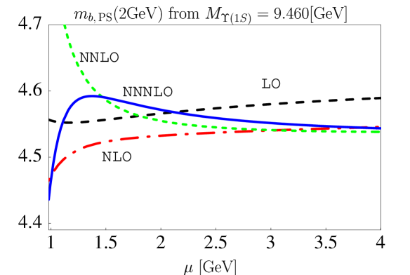
Figure 1: The bottom PS mass, $m_{b,\rm PS}(2\,\mbox{GeV})$, extracted from the experimental value $M_{\Upsilon(1S)}=9.460\,$GeV as a function of renormalization scale $\mu$ at LO (long dashes, black), NLO (long-short dashes, red), NNLO (short dashes, green) and NNNLO (solid, blue).

We can therefore use the experimental $\Upsilon(\rm{1S})$ mass $M_{\Upsilon(1S)}=9.460\,$GeV to extract the bottom PS mass at NNNLO as was done in [34] at NNLO. In Figure 1 we show the extracted PS mass as a function of the renormalization scale $\mu$ at LO (long dashes, black), NLO (long-short dashes, red), NNLO (short dashes, green) and NNNLO (solid, blue). Varying $\mu$ from $1.25\,$GeV to $4\,$GeV (as done in [34]) the NNNLO correction is never larger than about $30\,$MeV and the error from the scale dependence is of similar size. We therefore assign a $\pm 30\,$MeV error to $m_{b,\rm PS}$ from the truncation of the perturbative expansion. The uncertainty in $\alpha_{s}(M_{Z})=0.118\pm 0.003$ results in a $\pm 10\,$MeV error on $m_{b,\rm PS}$. The largest uncertainty in the determination of the bottom quark mass from the $\Upsilon(\rm{1S})$ mass is then from non-perturbative effects. The perturbative approximation is justified when the ultrasoft scale $m_{b}(C_{F}\alpha_{s})^{2}\gg\Lambda_{\rm QCD}$, in which case the leading non-perturbative contributions is expressed in terms of the gluon condensate [35, 36]

$$\delta M_{\Upsilon(1S)}^{\rm np}=\frac{624\pi m_{b}}{425}\,\frac{\langle\alpha_{s}GG\rangle}{(m_{b}C_{F}\alpha_{s})^{4}}.$$ (42)

The numerical estimate is strongly dependent on the choice of scale in $\alpha_{s}$ in the denominator. Referring to [34] for a more detailed discussion of the non-perturbative correction, we obtain

$$m_{b,\rm PS}(2\,\mbox{GeV})=(4.57\pm 0.03_{\rm pert.}\pm 0.01_{\alpha_{s}}\pm 0.07_{\rm non-pert.})\,\mbox{GeV}$$ (43)

as the final result of this analysis. Because of the small third-order correction the bottom quark mass remains practically unchanged compared to the second-order analysis of [34], and so does the $\overline{\rm MS}$ mass determined from (43). Further improvement of the mass determination by this method requires a quantitative understanding of non-perturbative effects.

Having determined $m_{b,\rm PS}$, we are in the position to predict the masses of the excited $S$-level states at the third order. (An analysis of the complete spectrum at second order was performed in [37].) We focus on the spin-triplet states $\Upsilon(\rm{2S})$ and $\Upsilon(\rm{3S})$. The successive approximations up to the third order are shown in Figure 2 for $m_{b,\rm PS}=4.57\,$GeV as a function of the renormalization scale. For $\mu$ between $2\,$GeV and $4\,$GeV it appears that the large third-order correction is welcome to bring the theoretical result closer to the observed masses. However, at the natural scales $1.23\,$GeV ($n=2$) and $0.98\,$GeV ($n=3$) the NNLO result agrees well with data and the NNNLO correction renders the prediction too large. As is apparent from the figure, the conclusion is that the perturbative computation of bottomonium masses is applicable only to the ground state, $n=1$, while the excited states, involving larger distances, appear to be in the non-perturbative regime. It can be seen from (39,40) that the NNNLO term for $n>1$ is dominated by the Coulomb correction.

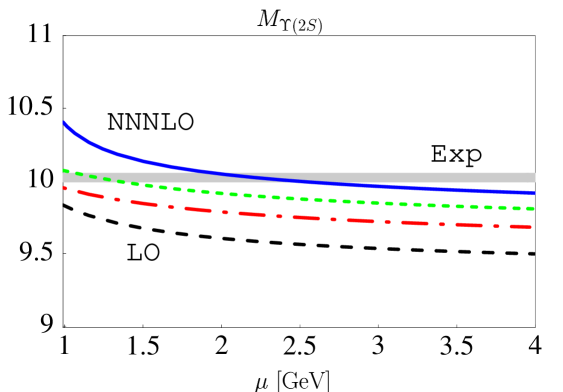
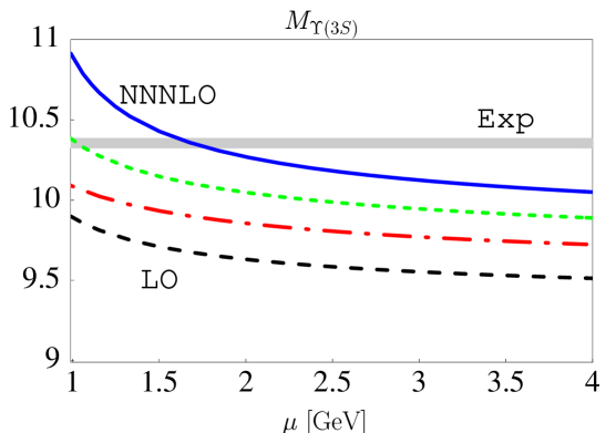
Figure 2: Predicted masses of the $\Upsilon(\rm{2S})$ and $\Upsilon(\rm{3S})$ as a function of the renormalization scale $\mu$. The lines refer to LO (long dashes, black), NLO (long-short dashes, red), NNLO (short dashes, green) and NNNLO (solid, blue). The widths of the bands for the experimental mass values are exaggerated.

4.2 Toponium

We briefly discuss the situation for the toponium masses. Toponium bound states do not exist in nature due to large decay width $\Gamma_{t}\sim 1.5\,$GeV of the top quark [38], however the remnant of the 1S toponium state should be visible as an enhancement in the cross section $e^{-}e^{+}\to t\bar{t}X$ near threshold. The convergence of the series expansion for the toponium 1S mass is therefore a good measure for the accuracy to which the top quark mass might be determined from this cross section [10].

The method suggested in [7, 29] relies on determining $m_{t,\rm PS}\equiv m_{t,\rm PS}(20\,\mbox{GeV})$ from the cross section measurement and obtaining the top quark $\overline{\rm MS}$ mass from $m_{t,\rm PS}$, since both relations are expected to be expressible in terms of well-behaved perturbative expansions. Adopting $m_{t,\rm PS}=175\,$GeV, $n_{f}=5$, $\Lambda_{\rm QCD}^{(n_{f}=5)}=208\,$MeV and the natural scale $\mu=32.6\,$GeV, where $L=0$, we obtain

$$M_{t\bar{t}(1S)}=(350+0.85+0.05-0.13+0.01)\,\mbox{GeV}=350.78\,\mbox{GeV}.$$ (44)

The sum of the series varies only by about $60\,$MeV when the scale is taken between $15\,$ and $60\,$GeV, although the convergence is no longer satisfactory at the lower scale. The small uncertainty implies that $m_{t,\rm PS}$ can be determined with little theoretical error from the cross section. The largest uncertainty in the determination of the top quark $\overline{\rm MS}$ mass then results from the unknown four-loop coefficient in the relation between the $\overline{\rm MS}$ mass and the pole mass, which is needed to convert $m_{t,\rm PS}$ to the $\overline{\rm MS}$ mass, as already observed in [7]. This uncertainty is estimated to be around $100\,$MeV (see Table 2 of [10]). Our conclusions are in good agreement with [39], where one of us investigated the direct determination of the top quark $\overline{\rm MS}$ mass from $M_{t\bar{t}(1S)}$ also using the NNNLO result for the 1S energy level. We should emphasize that none of these estimates take into account electroweak corrections, which are non-negligible, and must be included in the mass relations and cross section prediction before a comparison with the experimental cross section can be attempted.

5 Third-order Coulomb wave functions at the origin and Green function

In this section we turn to the discussion of the $S$-wave Coulomb Green function, and to the wave function of the origin squared (residues of the Green function at the bound state poles). Since the third-order correction is not completely known, we include in this section only the Coulomb corrections as defined in Section 3, i.e. we also neglect the (known) non-Coulomb correction at second order. The series expansions seem to be out of control for the wave functions in the bottomonium system, hence we focus on the case of the top quark and set $n_{f}=5$. We also set $a_{3}=a_{3,Pade}=3840$.

5.1 Wave function at origin squared

The numerical version of the general result for the $S$-state Coulomb wave function at the origin squared reads, for $n=1,2,3$,

$$\big{|}\psi_{1}(0)\big{|}^{2}_{C} = \frac{(m_{t}C_{F}\alpha_{s})^{3}}{8\pi}\bigg{[}1+\alpha_{s}\Big{(}-0.4333+3.661\,L\Big{)}+\alpha_{s}^{2}\Big{(}5.832-5.112\,L+8.933\,L^{2}\Big{)}$$ (45)

$$+\,\alpha_{s}^{3}\Big{(}-13.73+6.446\,\ln\left(\frac{\nu}{m_{t}C_{F}\alpha_{s}}\right)+39.72\,L-22.91\,L^{2}+18.17\,L^{3}\Big{)}\bigg{]},$$

$$\big{|}\psi_{2}(0)\big{|}^{2}_{C} = \frac{(m_{t}C_{F}\alpha_{s})^{3}}{64\pi}\bigg{[}1+\alpha_{s}\Big{(}-0.1769+3.661\,L\Big{)}+\alpha_{s}^{2}\Big{(}10.19-3.861\,L+8.933\,L^{2}\Big{)}$$ (46)

$$+\,\alpha_{s}^{3}\Big{(}-20.36+6.446\,\ln\left(\frac{2\nu}{m_{t}C_{F}\alpha_{s}}\right)+65.31\,L-19.09\,L^{2}+18.17\,L^{3}\Big{)}\bigg{]},$$

$$\big{|}\psi_{3}(0)\big{|}^{2}_{C} = \frac{(m_{t}C_{F}\alpha_{s})^{3}}{216\pi}\bigg{[}1+\alpha_{s}\Big{(}0.07953+3.661\,L\Big{)}+\alpha_{s}^{2}\Big{(}13.27-2.609\,L+8.933\,L^{2}\Big{)}$$ (47)

$$+\,\alpha_{s}^{3}\Big{(}-22.86+6.446\,\ln\left(\frac{3\nu}{m_{t}C_{F}\alpha_{s}}\right)+83.07\,L-15.27\,L^{2}+18.17\,L^{3}\Big{)}\bigg{]}\,.$$

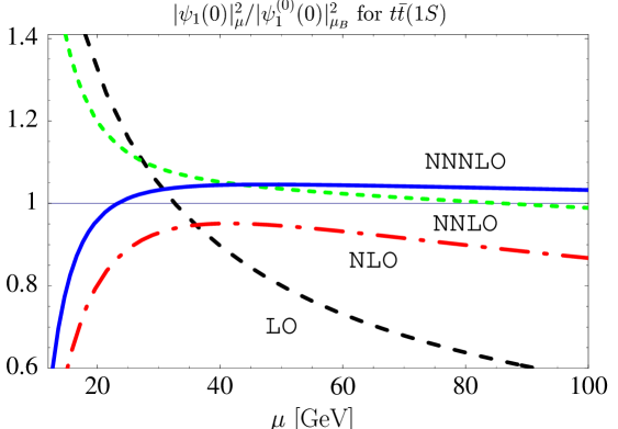
Figure 3: The Coulomb wave function at the origin squared for the ground state ($n=1$) normalized by $|\Psi_{1}^{(0)}(0)|^{2}$ at $\mu_{B}=32.6\,$GeV is shown as a function of the renormalization scale $\mu$. The input parameters are $m_{t,\rm PS}(20\,\mbox{GeV})=175\,$GeV, $\nu=m_{t,\rm PS}C_{F}\alpha_{s}(\mu)$. The lines refer to LO (long dashes, black), NLO (long-short dashes, red), NNLO (short dashes, green) and NNNLO (solid, blue).

We show the successive approximations for $n=1$ in Figure 3. As before, we re-expressed the expansion in terms of the PS mass, treating $\mu_{f}\sim m_{t}\alpha_{s}$. However, we note that contrary to the energy levels, the introduction of the PS mass does not change qualitatively the behaviour of the expansion, neither would this be expected on theoretical grounds. Our reference top quark mass is $m_{t,\rm PS}(20\,\mbox{GeV})=175\,$GeV, and the ultrasoft factorization scale is chosen to be $\nu=m_{t,\rm PS}C_{F}\alpha_{s}(\mu)$ such that the corresponding logarithm in (45) vanishes. We also normalized the result to the LO wave function at the scale $\mu_{B}\equiv m_{t,\rm PS}C_{F}\alpha_{s}(\mu_{B})=32.6\,$GeV. It is clearly seen from the figure that the approximations converge, and that the inclusion of the new third-order correction stabilizes the prediction further, provided $\mu$ is larger than about $25\,$GeV. We find a similar behaviour for $n=2,3$, where, however, the enhancement of the wave function relative to leading order is about $50\%$ ($n=2$) and $100\%$ ($n=3$) rather than roughly $5\%$ as at $n=1$.

It may be disconcerting that the perturbative expansion breaks down already at scales as large as $20\,$GeV, where the strong coupling is still small. A more detailed analysis shows that this early breakdown is caused primarily by the $\alpha_{s}(\alpha_{s}\beta_{0}\ln\mbox{\boldmath${q}$}^{2})^{n}$ terms in the Coulomb potential. We also note that at $\mu=\mu_{B}$, where $L=0$, the series expansions shown above are sign-alternating in contrast to the corresponding expressions for the energy levels, which exhibit fixed-sign behaviour. It is a general fact that for sign-alternating series of a certain regularity, the convergence of the expansion is much improved by choosing a larger scale [40], since this renders the series coefficients and the expansion parameter $\alpha_{s}$ smaller. This explains the stability seen in the figure towards scales larger than the natural scale $\mu=\mu_{B}$, and suggests that an error estimate for $|\psi_{n}(0)|^{2}$ from varying the scale between $\mu_{B}/2$ and $2\mu_{B}$ may be misleadingly large. We shall see in the following subsection that this is indeed the case.

5.2 Green function

In addition to the energy levels and wave functions at the origin we have also computed the full $S$-wave Green function up to the third order in the presence of the Coulomb potential as described in Section 2. The result is expressed in terms of multiple sums that can be evaluated numerically only.

The Coulomb Green function plays an important role in the calculation of inclusive top quark pair production $e^{-}e^{+}\to t\bar{t}X$ near threshold [41], since the bulk of the cross section is given by

$$R=\frac{\sigma_{t\overline{t}X}}{\sigma_{\mu^{+}\mu^{-}}}=\frac{18\pi e^{2}_{t}}{m_{t}^{2}}(1+a_{Z})\,\mathrm{Im}\,G(E+i\Gamma_{t})$$ (48)

where $e_{t}=2/3$ is the top quark electric charge, $\Gamma_{t}$ the top quark width, and $a_{Z}$ accounts for the vector coupling to the $Z$ boson. The convergence of the perturbative approximation up to the second order has been the subject of many investigations several years ago (see the review [10]).

We are now in the position to extend this investigation to the third order as far as the corrections from the Coulomb potential are concerned. We computed the perturbative expansion of the Green function given in (6). This strict expansion is never a good approximation, because it contains terms of the form

$$\left[\frac{\alpha_{s}E_{n}^{(0)}}{E_{n}^{(0)}-(E+i\Gamma_{t})}\right]^{k},$$ (49)

which originate from the expansion of (7) around $E_{n}^{(0)}$ rather than the true pole position. These terms become numerically large near $E\approx E_{n}^{(0)}$, but they can be summed by adding the exact pole structure and subtracting the expanded structure to the appropriate order, see [7] for the corresponding expressions. In the following, “perturbative approximation” means that this resummation is included. Alternatively, we computed the Green function (5) numerically by solving the Schrödinger equation with the Coulomb potential (4) exactly, following the method described in [42]. We shall refer to this as the “exact result”. The exact result contains an arbitrary number of insertions of the perturbation potentials $\delta V_{1}$, $\delta V_{2}$, $\delta V_{3}$. The leading difference to the third-order perturbative approximation consists of fourth-order terms of the form $\hat{G}_{0}\delta V_{1}\hat{G}_{0}\delta V_{1}\hat{G}_{0}\delta V_{1}\hat{G}_{0}\delta V_{1}\hat{G}_{0}$, $\hat{G}_{0}\delta V_{1}\hat{G}_{0}\delta V_{1}\hat{G}_{0}\delta V_{2}\hat{G}_{0}$ etc. Comparing the two results we obtain an estimate of the importance of these multiple insertions and of the convergence of the perturbative approximation.

For the following numerical study we assume $\Lambda^{(n_{f}=5)}_{\rm QCD}=0.208\,$GeV ($\alpha_{s}(M_{Z})=0.118$), four-loop evolution of $\alpha_{s}$, $\Gamma_{t}=1.5$GeV, and $\nu=20\,$GeV. It is crucial for an accurate prediction of the cross section not to use the top quark pole mass as an input parameter [7, 10]. Our result is presented in terms of the top-quark potential-subtracted mass $m_{t,\rm PS}(20\,\mbox{GeV})=175\,$GeV defined in (37). The conversion to the top quark $\overline{\rm MS}$ mass is given in [10]. We implement the PS scheme by working with an order-dependent pole mass. That is, in the N^kLO perturbative approximation we compute the top quark pole mass $m_{t}^{(k)}$ from $m_{t,\rm PS}(20\,\mbox{GeV})=175\,$GeV according to (37) including the terms up to order $\mu_{f}\alpha^{k+1}_{s}$, and use $m_{t}^{(k)}$ as an input to the Green function. For instance, for renormalization scale $\mu=30\,$GeV we obtain $m_{t}^{(k)}=(176.21,176.56,176.74,176.87)\,$GeV for $k=0,1,2,3$. The energy argument of the Green function is then

$$E=\sqrt{s}-2m_{t}^{(k)}$$ (50)

with $\sqrt{s}$ the center-of-mass energy of the $e^{-}e^{+}$ collision.

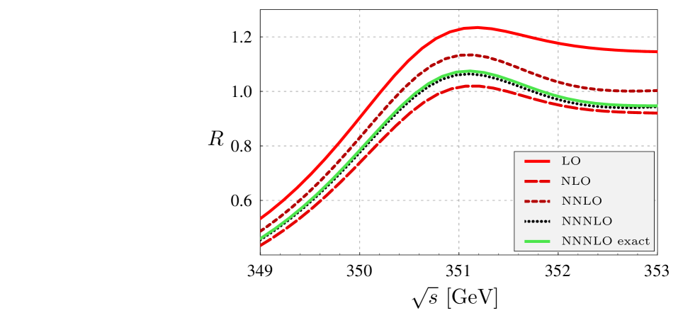
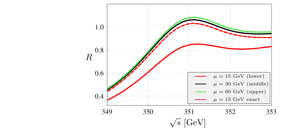
Figure 4: Top quark pair production cross section (Coulomb corrections only) for $m_{t,\rm PS}=175\,$GeV, $\Gamma_{t}=1.5\,$GeV. Upper panel: successive approximations up to the third order for $\mu=30\,$GeV. Lower panel: Scale dependence of the third-order approximation. See text for further explanation.

The upper plot in Figure 4 shows the convergence of the successive perturbative approximations to the exact result for the Green function (cross section) at the renormalization scale $\mu=30\,$GeV. The location of the “peak” position is indeed stable under the inclusion of higher-order corrections as expected in the PS scheme. On the other hand, the corrections to the magnitude of the cross section near the peak are significant, decreasing from about $20\%$ at NLO to about $7\%$ at NNNLO. The corrections alternate in sign as expected from the behaviour of the series expansion of $|\psi_{1}(0)|^{2}$. An important observation is that the third-order perturbative approximation coincides with the exact result within $1\%$. Hence the higher-order insertions of the perturbation potentials are negligible. The convergence of the approximations then suggests that the residual error from yet higher perturbation Coulomb potentials $\delta V_{4}$ etc. should be less than $5\%$.

In the lower plot of Figure 4 we display the renormalization scale dependence of the third-order perturbative approximation (solid lines, $\mu=(60,30,15)\,$GeV from top to bottom). It is immediately apparent that the scale dependence is very small from $30$ to $60\,$GeV, but the result for $\mu=15\,$GeV is far away. We can trace this anomalous behaviour directly to the breakdown of the perturbative expansion for $|\psi_{1}(0)|^{2}$ at scales below $25\,$GeV discussed in the previous subsection and displayed in Figure 3. The exact result (dashed line) does not exhibit this behaviour for $\mu=15\,$GeV, hence we conclude that the multiple insertions of the perturbation potentials become large at small scales and destroy the agreement of the perturbative and exact result. Indeed, we find that the series of multiple insertions is very slowly converging at small scales. We therefore learn the important lesson that the “correct” choice of scale in the perturbative approach is $\mu>25\,$GeV, while choosing smaller scales would lead to misleadingly large uncertainties. The lower plot of Figure 4 indicates that the scale dependence is less than $5\%$, similar in size to the truncation error estimated above. This discussion does not include the unknown third-order non-Coulomb corrections, but it lends support to the optimistic interpretation that the magnitude of the $t\bar{t}$ threshold cross section can eventually be computed with an accuracy of a few percent.

6 Conclusion

We computed the third-order corrections from the strong interaction Coulomb potential to the energy levels and the wave functions at the origin of the $S$-waves bound states, and to the expectation value of the $S$-wave Green function operator in the $|\mbox{\boldmath${r}$}=\mbox{\boldmath${0}$}\rangle$ state. We view this as a first step towards a complete calculation of the third-order top quark pair production cross section $e^{-}e^{+}\to t\bar{t}X$ near threshold. It also completes the expression for the $S$-wave quarkonium masses with accuracy $m\alpha_{s}^{5}$ for arbitrary principal quantum number $n$, except for the unknown constant $a_{3}$ in the Coulomb potential.

We updated the determination of the bottom quark mass from the mass of the $\Upsilon(\rm{1S})$ and obtain

$$m_{b,\rm PS}(2\,\mbox{GeV})=(4.57\pm 0.03_{\rm pert.}\pm 0.01_{\alpha_{s}}\pm 0.07_{\rm non-pert.})\,\mbox{GeV}$$ (51)

for the PS mass, with almost no modification compared to the second-order analysis [34]. Our numerical study of the Coulomb corrections to the top quark pair production cross section near threshold shows that the perturbative approach (mandatory once non-Coulomb corrections are included) works and led to the conclusion that the residual uncertainty from the Coulomb corrections is less than $5\%$. This lends support to the optimistic interpretation that the magnitude of the $t\bar{t}$ threshold cross section can eventually be computed with an accuracy of a few percent.

Note added

During the preparation of this paper Penin, Smirnov and Steinhauser [25] have obtained results for the Coulomb correction to the second and third energy level and wave function at the origin ($n=2,3$), which agree with our result for general $n$. We thank the authors for communicating and comparing their results prior to publication.

Acknowledgements

This work was supported by the DFG Sonderforschungsbereich/Transregio 9 “Computer-gestützte Theoretische Teilchenphysik”. K.S. acknowledges support of the DFG Graduiertenkolleg “Elementarteilchenphysik an der TeV-Skala”.

Appendix

The most difficult part of the third-order calculation of the Green function is the threefold insertion $\langle 0|\hat{G}_{0}\delta V_{1}\hat{G}_{0}\delta V_{1}\hat{G}_{0}\delta V_{1}\hat{G}_{0}|0\rangle$ of the first-order perturbation potential

$$\delta\tilde{V}_{1}(\mbox{\boldmath${q}$})=-\frac{4\pi C_{F}\alpha_{s}}{\mbox{\boldmath${q}$}^{2}}\frac{\alpha_{s}}{4\pi}\bigg{[}a_{1}+\beta_{0}\ln\frac{\mu^{2}}{\mbox{\boldmath${q}$}^{2}}\bigg{]}.$$ (52)

The matrix element is ultraviolet and infrared finite, so the computation can be done in three dimensions. Since the external state is a position eigenstate, we Fourier transform to position space, where the potential has a $1/r$ and a $\ln(r)/r$ term. We can generate these terms by working with

$$W_{i}(\mbox{\boldmath${r}$}_{i}) = \frac{1}{4\pi\Gamma(1+2u_{i})\cos(\pi u_{i})}\left(\mbox{\boldmath${r}$}_{i}^{2}\right)^{u_{i}-\frac{1}{2}}$$ (53)

and by taking the zeroth and first derivative with respect to the $u_{i}$ at $u_{i}=0$. The threefold insertion of the generating potential reads

$$J_{3} \equiv \int\prod_{i=1}^{3}d^{3}\mbox{\boldmath${r}$}_{i}\,G_{0}(0,\mbox{\boldmath${r}$}_{1};E)W_{1}(\mbox{\boldmath${r}$}_{1})G_{0}(\mbox{\boldmath${r}$}_{1},\mbox{\boldmath${r}$}_{2};E)W_{2}(\mbox{\boldmath${r}$}_{2})G_{0}(\mbox{\boldmath${r}$}_{2},\mbox{\boldmath${r}$}_{3};E)W_{3}(\mbox{\boldmath${r}$}_{3})G_{0}(\mbox{\boldmath${r}$}_{3},0;E)$$ (54)

$$= \int dr_{1}dr_{2}dr_{3}\,\frac{r_{1}^{2u_{1}+1}}{\Gamma(1+2u_{1})\cos(\pi u_{1})}\frac{r_{2}^{2u_{2}+1}}{\Gamma(1+2u_{2})\cos(\pi u_{2})}\frac{r_{3}^{2u_{3}+1}}{\Gamma(1+2u_{3})\cos(\pi u_{3})}$$

$$\times\bigg{\{}G_{0}(0,r_{1},E)G_{0}^{(l=0)}(r_{1},r_{2},E)G_{0}^{(l=0)}(r_{2},r_{3},E)G_{0}(0,r_{3},E)\bigg{\}}.$$

For the zeroth-order $S$-wave Coulomb Green functions we use the representations [43, 44]

$$G_{0}(0,r_{i},E)=-\frac{im^{2}v}{2\pi}e^{imvr_{i}}\int_{0}^{\infty}dt\,e^{2imvr_{i}t}\left(\frac{1+t}{t}\right)^{\!\lambda},$$ (55)

$$G_{0}^{(l=0)}(r_{i},r_{j},E) = -\frac{im^{2}v}{2\pi}\,e^{imv(r_{i}+r_{j})}\sum_{n=0}^{\infty}\frac{L_{n}^{(1)}(-2imvr_{i})L_{n}^{(1)}(-2imvr_{j})}{(n+1)(n+1-\lambda)}$$ (56)

with $v\equiv\sqrt{(E+i\epsilon)/m}$ and $\lambda=iC_{F}\alpha_{s}/(2v)$. The $L_{n}^{(l)}(x)$ are the Laguerre polynomials. The integrals over $r_{i}$ can now be factorized into two functions $H(u,n)$ and $K(u,n,j)$, and we obtain

$$J_{3} = \left(\frac{m}{4\pi}\right)^{4}\sum_{n=0}^{\infty}\sum_{j=0}^{\infty}\frac{H(u_{1},n)K(u_{2},n,j)H(u_{3},j)}{(n+1)(n+1-\lambda)(j+1)(j+1-\lambda)},$$ (57)

where (defining $s=-2imvr$)

$$H(u,n) \equiv \frac{1}{\Gamma(1+2u)\cos\pi u}\left(\frac{e^{i\pi}}{4m^{2}v^{2}}\right)^{\!u}\int_{0}^{\infty}\!dt\left(\frac{1+t}{t}\right)^{\!\lambda}\int_{0}^{\infty}\!ds\,e^{-(1+t)s}s^{2u+1}L_{n}^{(1)}(s),\phantom{mov}$$ (58)

$$K(u,n,j) \equiv \frac{1}{\Gamma(1+2u)\cos(\pi u)}\frac{-1}{4m^{2}v^{2}}\left(\frac{e^{i\pi}}{4m^{2}v^{2}}\right)^{u}\int_{0}^{\infty}\!ds\,s^{2u+1}e^{-s}L_{n}^{(1)}(s)L_{j}^{(1)}(s).$$ (59)

Performing the integrations in $H(u,n)$ (substituting $x=1/(1+t)$ in the $t$-integral), we find

$$H(u,n) = (-4mE)^{-u}\frac{(1+2u)(n+1)}{\cos(\pi u)}\int_{0}^{\infty}dt\,t^{-\lambda}(1+t)^{\lambda-2-2u}\,_{2}F_{1}\left(-n,2+2u;2;\frac{1}{1+t}\right)$$ (60)

$$= \frac{(n+1)\Gamma(1-\lambda)}{\cos(\pi u)(-4mE)^{u}}\sum_{k=0}^{n}\frac{(-1)^{k}n!}{k!(n-k)!}\frac{\Gamma(2+k+2u)\Gamma(1+k+2u)}{\Gamma(1+2u)\Gamma(k+2)\Gamma(2+k+2u-\lambda)}.$$

The sum can be expressed in terms of the hypergeometric function ${}_{3}F_{2}(-n,2+2u,1+2u;2,2+2u-\lambda;1)$, but it is simpler to perform the expansion in the generating variable $u$ directly. We need the first two terms in the expansion. With the help of the generating sum

$$\sum_{k=0}^{n}\frac{(-1)^{k}n!}{k!(n-k)!}\frac{\Gamma(1+k+a)}{\Gamma(2+k-\lambda)}=\frac{\Gamma(1+a)\Gamma(1-a+n-\lambda)}{\Gamma(2+n-\lambda)\Gamma(1-a-\lambda)}$$ (61)

we find

$$H(0,n) = \frac{n+1}{n+1-\lambda},$$ (62)

$$H^{\prime}(0,n) = (n+1)\Gamma(1-\lambda)\sum_{k=0}^{n}\frac{(-1)^{k}n!}{k!(n-k)!}\frac{\Gamma(1+k)}{\Gamma(2+k-\lambda)}\bigg{\{}2\gamma_{E}-\ln(-4mE)$$ (63)

$$+\,2\Psi(1+k)+2\Psi(2+k)-2\Psi(2+k-\lambda)\bigg{\}}$$

$$= \frac{n+1}{n+1-\lambda}\bigg{\{}\!-\ln(-4mE)-2\Big{[}\gamma_{E}+\Psi(n+1-\lambda)\Big{]}$$

$$\hskip 59.75095pt+\,\frac{2\lambda}{(n+1)}\Big{[}\Psi(1-\lambda)-\Psi(n+2-\lambda)\Big{]}\bigg{\}},$$

where $\Psi(z)$ denotes Euler’s Psi-function, and $\gamma_{E}=0.577216\ldots$ is Euler’s constant. This result has already been obtained in [7].

Similarly, for $K(u,n,j)$ we need the expansion up to the first order in $u$. Here we obtain

$$K(0,n,j) = -\frac{n+1}{4m^{2}v^{2}}\,\delta_{nj},$$ (64)

$$K^{\prime}(0,n,j) = -\frac{1}{4m^{2}v^{2}}\Big{[}I+(n+1)\,\delta_{nj}\left(2\gamma_{E}-\ln(-4mE)\right)\Big{]}$$ (65)

with

$$I = \int_{0}^{\infty}ds\,2s\ln(s)e^{-s}L_{n}^{(1)}(s)L_{j}^{(1)}(s).$$ (66)

To solve the integral $I$, the Laguerre polynomials are expressed through their generating functions. Then with

$$\frac{e^{-\frac{z\,u}{1-u}}}{(1-u)^{2}}=\sum_{s=0}^{\infty}u^{s}L_{s}^{(1)}(z),$$ (67)

and

$$\int_{0}^{\infty}ds\,2s\ln(s)e^{-s}\frac{e^{-\frac{s\,v}{1-v}}}{(1-v)^{2}}\frac{e^{-\frac{s\,w}{1-w}}}{(1-w)^{2}}=-\frac{2\Big{[}-1+\gamma_{E}+\ln\left(\frac{1-vw}{(v-1)(w-1)}\right)\Big{]}}{(vw-1)^{2}},$$ (68)

the integral $I$ is expressed as

$$I = \frac{1}{n!}\frac{1}{j!}\frac{\partial^{n}}{\partial v^{n}}\frac{\partial^{j}}{\partial w^{j}}\left[-\frac{2\left(-1+\gamma_{E}+\ln\left(\frac{1-vw}{(v-1)(w-1)}\right)\right)}{(vw-1)^{2}}\right]_{v=w=0}$$ (71)

$$= \left\{\begin{array}[]{cc}2+2(1+n)\Psi(1+n)&\hskip 11.38092pt\textrm{if}\;n=j\\[5.69046pt] -2\frac{\displaystyle\min(n,j)+1}{\displaystyle|j-n|}&\hskip 11.38092pt\textrm{if}\;n\neq j\\ \end{array}\right.$$

Hence the final result for $K^{\prime}(0,n,j)$ reads

$$K^{\prime}(0,n,j) = -\frac{1}{4m^{2}v^{2}}\left\{\begin{array}[]{cc}2+(n+1)\Big{\{}2[\gamma_{E}+\Psi(1+n)]-\ln(-4mE)\Big{\}}&\hskip 11.38092pt\textrm{if}\;n=j\hskip 22.76228pt\\[5.69046pt] -2\,\frac{\displaystyle\min(n,j)+1}{\displaystyle|j-n|}&\hskip 11.38092pt\textrm{if}\;n\neq j\hskip 22.76228pt\end{array}\right.$$ (74)

At this point, we have expressed the threefold insertion of the perturbation potential in terms of a doubly infinite sum involving Euler’s Psi-function, see (57) . These sums converge rapidly when the energy argument is evaluated along a line parallel to the real axis as required in the calculation of the top quark pair production cross section. In order to obtain the third-order correction to the energy levels and wave functions at the origin in Section 3, we extract analytically the pole part of $J_{3}$ when $E$ approaches the leading-order $S$-wave bound state energies $E_{n}^{(0)}$, which correspond to $\lambda=n$. This results in multiple sums, which, after a tedious reduction, can all be expressed in terms of zeta-functions and nested harmonic sums.

References

• [1] M. Beneke, A. Signer and V. A. Smirnov, Phys. Rev. Lett.  80 (1998) 2535 [hep-ph/9712302].
• [2] A. Czarnecki and K. Melnikov, Phys. Rev. Lett.  80 (1998) 2531 [hep-ph/9712222].
• [3] Y. Schröder, Phys. Lett. B 447 (1999) 321 [hep-ph/9812205].
• [4] A. Pineda and F. J. Yndurain, Phys. Rev. D 58 (1998) 094022 [hep-ph/9711287].
• [5] K. Melnikov and A. Yelkhovsky, Phys. Rev. D 59 (1999) 114009 [hep-ph/9805270].
• [6] A. A. Penin and A. A. Pivovarov, Nucl. Phys. B 549 (1999) 217 [hep-ph/9807421].
• [7] M. Beneke, A. Signer and V. A. Smirnov, Phys. Lett. B 454 (1999) 137 [hep-ph/9903260].
• [8] A. H. Hoang and T. Teubner, Phys. Rev. D 58, 114023 (1998) [hep-ph/9801397].
• [9] K. Melnikov and A. Yelkhovsky, Nucl. Phys. B 528 (1998) 59 [hep-ph/9802379].
• [10] A. H. Hoang et al., Eur. Phys. J. directC 2 (2000) 3 [hep-ph/0001286].
• [11] For a review, see M. Beneke, Perturbative heavy quark-antiquark systems, [hep-ph/9911490].
• [12] M. Beneke, Phys. Lett. B 434 (1998) 115 [hep-ph/9804241].
• [13] N. Brambilla, A. Pineda, J. Soto and A. Vairo, Phys. Rev. D 60 (1999) 091502 [hep-ph/9903355].
• [14] B. A. Kniehl and A. A. Penin, Nucl. Phys. B 563 (1999) 200 [hep-ph/9907489].
• [15] N. Brambilla, A. Pineda, J. Soto and A. Vairo, Phys. Lett. B 470 (1999) 215 [hep-ph/9910238].
• [16] Y. Kiyo and Y. Sumino, Phys. Lett. B 496 (2000) 83 [hep-ph/0007251].
• [17] A. H. Hoang, [hep-ph/0008102].
• [18] B. A. Kniehl, A. A. Penin, V. A. Smirnov and M. Steinhauser, Nucl. Phys. B 635 (2002) 357 [hep-ph/0203166].
• [19] B. A. Kniehl and A. A. Penin, Nucl. Phys. B 577 (2000) 197 [hep-ph/9911414].
• [20] A. V. Manohar and I. W. Stewart, Phys. Rev. D 63 (2001) 054004 [hep-ph/0003107].
• [21] A. H. Hoang, Phys. Rev. D 69 (2004) 034009 [hep-ph/0307376].
• [22] B. A. Kniehl, A. A. Penin, M. Steinhauser and V. A. Smirnov, Phys. Rev. Lett.  90 (2003) 212001 [hep-ph/0210161].
• [23] A. H. Hoang, A. V. Manohar, I. W. Stewart and T. Teubner, Phys. Rev. D 65 (2002) 014014 [hep-ph/0107144].
• [24] A. A. Penin and M. Steinhauser, Phys. Lett. B 538 (2002) 335 [hep-ph/0204290].
• [25] A. A. Penin, V. A. Smirnov and M. Steinhauser, [hep-ph/0501042].
• [26] T. van Ritbergen, J. A. M. Vermaseren and S. A. Larin, Phys. Lett. B 400 (1997) 379 [hep-ph/9701390].
• [27] F. A. Chishtie and V. Elias, Phys. Lett. B 521 (2001) 434 [hep-ph/0107052].
• [28] A. Pineda and J. Soto, Nucl. Phys. Proc. Suppl.  64 (1998) 428 [hep-ph/9707481].
• [29] M. Beneke, in: Proceedings of the XXXIIIrd Rencontres de Moriond, ’98 Electroweak Interactions and Unified Theories, J. Tran Thanh Van (Ed.), Editions Frontieres, Paris [hep-ph/9806429].
• [30] T. Appelquist, M. Dine and I. J. Muzinich, Phys. Rev. D 17 (1978) 2074.
• [31] I. I. Y. Bigi, M. A. Shifman, N. G. Uraltsev and A. I. Vainshtein, Phys. Rev. D 50, 2234 (1994) [hep-ph/9402360].
• [32] M. Beneke and V. M. Braun, Nucl. Phys. B 426 (1994) 301 [hep-ph/9402364].
• [33] A. H. Hoang, M. C. Smith, T. Stelzer and S. Willenbrock, Phys. Rev. D 59, 114014 (1999) [hep-ph/9804227].
• [34] M. Beneke and A. Signer, Phys. Lett. B 471 (1999) 233 [hep-ph/9906475].
• [35] H. Leutwyler, Phys. Lett. B 98 (1981) 447.
• [36] M.B. Voloshin, Sov. J. Nucl. Phys. 36(1) (1982) 143.
• [37] N. Brambilla, Y. Sumino and A. Vairo, Phys. Lett. B 513 (2001) 381 [hep-ph/0101305].
• [38] I. I. Y. Bigi, Y. L. Dokshitzer, V. A. Khoze, J. H. Kühn and P. M. Zerwas, Phys. Lett. B 181 (1986) 157.
• [39] Y. Kiyo and Y. Sumino, Phys. Rev. D 67 (2003) 071501 [hep-ph/0211299].
• [40] M. Beneke and V. I. Zakharov, Phys. Rev. Lett.  69 (1992) 2472.
• [41] V.S. Fadin and V.A. Khoze, Pis’ma Zh. Eksp. Teor. Fiz. 46, 417 (1987) [JETP Lett. 46, 525 (1987)]; Yad. Fiz. 48, 487 (1988) [Sov. J. Nucl. Phys. 48(2), 309 (1988)].
• [42] M. J. Strassler and M. E. Peskin, Phys. Rev. D 43 (1991) 1500.
• [43] E.H. Wichmann and C.H. Woo, J. Math. Phys. 2 (1961) 178.
• [44] M. B. Voloshin, Sov. J. Nucl. Phys.  40 (1984) 662 [Yad. Fiz.  40 (1984) 1039].