Signatures of Axinos and Gravitinos at Colliders

Abstract

The axino and the gravitino are well-motivated candidates for the lightest supersymmetric particle (LSP) and also for cold dark matter in the Universe. Assuming that a charged slepton is the next-to-lightest supersymmetric particle (NLSP), we show how the NLSP decays can be used to probe the axino LSP scenario in hadronic axion models as well as the gravitino LSP scenario at the Large Hadron Collider and the International Linear Collider. We show how one can identify experimentally the scenario realized in nature. In the case of the axino LSP, the NLSP decays will allow one to estimate the value of the axino mass and the Peccei–Quinn scale.

I Introduction

In supersymmetric extensions of the Standard Model with unbroken R-parity Nilles:1983ge+X , the lightest supersymmetric particle (LSP) is stable and plays an important role in both collider phenomenology and cosmology. The most popular LSP candidate is the lightest neutralino, which appears already in the Minimal Supersymmetric Standard Model (MSSM). Here we consider two well-motivated alternative LSP candidates, which are not part of the spectrum of the MSSM: the axino and the gravitino. In particular, either of them could provide the right amount of cold dark matter in the Universe if heavier than about 1 MeV (see Covi:1999ty+X ; Brandenburg:2004du+X and Moroi:1993mb ; Bolz:1998ek+X ; Fujii:2002fv+X ; Feng:2003xh+X ; Roszkowski:2004jd , respectively, and references therein).

The axino Nilles:1981py+X ; Tamvakis:1982mw ; Kim:1983ia appears (as the spin-1/2 superpartner of the axion) when extending the MSSM with the Peccei–Quinn mechanism Peccei:1977hh+X in order to solve the strong CP problem. Depending on the model and the supersymmetry (SUSY) breaking scheme, the mass of the axino can range between the eV and the GeV scale Tamvakis:1982mw ; Nieves:1985fq+X ; Rajagopal:1990yx ; Goto:1991gq+X .

The gravitino appears (as the spin-3/2 superpartner of the graviton) once SUSY is promoted from a global to a local symmetry leading to supergravity (SUGRA) Wess:1992cp . The mass of the gravitino depends strongly on the SUSY-breaking scheme and can range from the eV scale to scales beyond the TeV region Nilles:1983ge+X ; Dine:1994vc+X ; Randall:1998uk+X . In particular, in gauge-mediated SUSY breaking schemes Dine:1994vc+X , the gravitino mass is typically less than 100 MeV, while in gravity-mediated schemes Nilles:1983ge+X it is expected to be in the GeV to TeV range.

Both the axino and the gravitino are singlets with respect to the gauge groups of the Standard Model. Both interact extremely weakly as their interactions are suppressed by the Peccei–Quinn scale Sikivie:1999sy ; Eidelman:2004wy $f_{a}\buildrel>\over{{}_{\sim}}5\times 10^{9}\,\mbox{GeV}$ and the (reduced) Planck scale Eidelman:2004wy $\mathrm{M}_{\mathrm{Pl}}=2.4\times 10^{18}\,\mbox{GeV}$, respectively. Therefore, in both the axino LSP and the gravitino LSP cases, the next-to-lightest supersymmetric particle (NLSP) typically has a long lifetime. For example, for axino cold dark matter, an NLSP with a mass of 100 GeV has a lifetime of ${\cal O}$(1 sec). For gravitino cold dark matter, this lifetime is of ${\cal O}$(1 sec) for a gravitino mass of 10 MeV and of ${\cal O}(10^{6}~{}\mbox{sec})$ for a gravitino mass of 10 GeV. Late NLSP decays can spoil successful predictions of primordial nucleosynthesis and can distort the CMB blackbody spectrum. Constraints are obtained in order to avoid the corresponding (rather mild) axino problem or the more severe and better-known gravitino problem. In the axino LSP case, either a neutralino or a slepton could be the NLSP Covi:2004rb . In the gravitino LSP case, these constraints strongly disfavour a bino-dominated neutralino NLSP, while a slepton NLSP remains allowed Fujii:2003nr+X ; Roszkowski:2004jd .

Because of their extremely weak interactions, the direct detection of axinos and gravitinos seems hopeless. Likewise, their direct production at colliders is very strongly suppressed. Instead, one expects a large sample of NLSPs from pair production or cascade decays of heavier superparticles, provided the NLSP belongs to the MSSM spectrum. These NLSPs will appear as quasi-stable particles, which will eventually decay into the axino/gravitino LSP. A significant fraction of these NLSP decays will take place outside the detector and will thus escape detection. For the charged slepton NLSP scenario, however, there have recently been proposals, which discuss the way such NLSPs could be stopped and collected for an analysis of their decays into the LSP. It was found that up to ${\cal O}(10^{3}$–$10^{4})$ and ${\cal O}(10^{3}$–$10^{5})$ of charged NLSPs can be trapped per year at the Large Hadron Collider (LHC) and the International Linear Collider (ILC), respectively, by placing 1–10 kt of massive additional material around planned collider detectors Hamaguchi:2004df ; Feng:2004yi .

In this Letter we assume that the NLSP is a charged slepton. In Sec. II we investigate the NLSP decays in the axino LSP scenario. These decays were previously considered in Covi:2004rb . We show that the NLSP decays can be used to estimate the axino mass and to probe the Peccei–Quinn sector. In particular, we obtain a new method to measure the Peccei–Quinn scale $f_{a}$ at future colliders.

In Sec. III we consider the corresponding NLSP decays in the gravitino LSP scenario. These decays were already studied in Buchmuller:2004rq . It was shown that the measurement of the NLSP lifetime can probe the gravitino mass and can lead to a new (microscopic) determination of the Planck scale with an independent kinematical reconstruction of the gravitino mass. Moreover, it was demonstrated that slepton NLSP decays into the corresponding lepton, the gravitino, and the photon can be used to reveal the peculiar couplings and possibly even the spin of the gravitino. In Ref. Buchmuller:2004rq the limit of an infinite neutralino mass was used. Here we generalize the result obtained therein for the three-body decay by taking into account finite values of the neutralino mass.

A question arises as to whether one can distinguish between the axino LSP and the gravitino LSP scenarios at colliders. From the NLSP lifetime alone, such a distinction will be difficult, in particular if the mass of the LSP cannot be determined. Thus, an analysis of the three-body decay of the charged NLSP slepton into the corresponding lepton, the LSP, and a photon will be essential. With a measurement of the polarizations of the final-state lepton and photon, the determination of the spin of the LSP should be possible Buchmuller:2004rq and would allow us to decide clearly between the spin-1/2 axino and the spin-3/2 gravitino. The spin measurement, however, will be very difficult. In Sec. IV we present more feasible methods to distinguish between the axino LSP and the gravitino LSP scenarios, which are also based on the analysis of the three-body NLSP decay with a lepton and a photon in the final state.

Let us comment on the mass hierarchy of the relevant particles. There are six possible orderings in the hierarchy of the axino mass $m_{{\widetilde{a}}}$, the gravitino mass $m_{\widetilde{G}}$, and the mass of the lightest ordinary supersymmetric particle (LOSP) $m_{\mathrm{LOSP}}$. Here the LOSP is the lightest charged slepton. The cases relevant in this Letter are (i) $m_{{\widetilde{a}}}<m_{\mathrm{LOSP}}<m_{\widetilde{G}}$, (ii) $m_{\widetilde{G}}<m_{\mathrm{LOSP}}<m_{{\widetilde{a}}}$, (iii) $m_{{\widetilde{a}}}<m_{\widetilde{G}}<m_{\mathrm{LOSP}}$, and (iv) $m_{\widetilde{G}}<m_{{\widetilde{a}}}<m_{\mathrm{LOSP}}$. In cases (iii) and (iv), the LOSP has two distinct decay channels, one into the axino and the other into the gravitino. However, unless the decay rates into the axino and the gravitino are (accidentally) comparable, the phenomenology of the LOSP decay in the cases (iii) and (iv) can essentially be reduced to the cases (i) or (ii), although not necessarily respectively, as will be discussed in Sec. IV. We will thus concentrate on the cases (i) and (ii) and call the LOSP the NLSP.

II Axino LSP Scenario

In this section we consider the axino LSP scenario. The relevant interactions of the axino are discussed. The rates of the two-body and three-body decays of the charged slepton NLSP are given. We demonstrate that these decays can be used to estimate the Peccei–Quinn scale and the axino mass.

To be specific, we focus on the case where the lighter stau ${\widetilde{\tau}}$ is the NLSP. In general, the stau is a linear combination of ${\widetilde{\tau}}_{\mathrm{R}}$ and ${\widetilde{\tau}}_{\mathrm{L}}$, which are the superpartners of the right-handed and left-handed tau lepton, respectively: ${\widetilde{\tau}}=\cos\theta_{\tau}{\widetilde{\tau}}_{\mathrm{R}}+\sin\theta_{\tau}{\widetilde{\tau}}_{\mathrm{L}}$. For simplicity, we concentrate on a pure ‘right-handed’ stau ${\widetilde{\tau}}_{\mathrm{R}}$, which is a good approximation at least for small $\tan\beta$. Then, the neutralino–stau coupling is dominated by the bino coupling. In addition, we assume for simplicity that the lightest neutralino is a pure bino.

II.1 Axino Interactions

Let us first discuss how the axino couples to the stau. Concentrating on hadronic, or KSVZ, axion models Kim:1979if+X in a SUSY setting, the coupling of the axino to the bino and the photon/Z-boson at scales below the Peccei–Quinn scale $f_{a}$ is given effectively by the Lagrangian Covi:1999ty+X

$${\cal L}_{{\widetilde{a}}} = i\,\frac{\alpha_{\mathrm{Y}}C_{\rm aYY}}{16\pi f_{a}}\,{\overline{\tilde{a}}}\,\gamma_{5}\,[\gamma_{\mu},\gamma_{\nu}]\,{\widetilde{B}}\,\left(\cos\theta_{W}F_{\mu\nu}-\sin\theta_{W}Z_{\mu\nu}\right),$$ (1)

where $\theta_{W}$ is the weak mixing angle, $\alpha_{\mathrm{Y}}=\alpha/\cos^{2}\theta_{W}$ with the fine structure constant $\alpha$, and $F_{\mu\nu}$ and $Z_{\mu\nu}$ are the field strength tensors of the photon and Z-boson, respectively. The interaction Lagrangian (1) is obtained by integrating out the heavy (s)quarks introduced in supersymmetric KSVZ axion models. Indeed, the KSVZ axino couples directly only to these additional heavy (s)quarks. Thus, the above coupling depends, for example, on the hypercharge of these heavy (s)quarks, which we assume to be non-zero. The model dependence related to the Peccei–Quinn sector is expressed in terms of the factor $C_{\rm aYY}\simeq\mathcal{O}(1)$. As the MSSM fields do not carry Peccei–Quinn charges, the axino couples to the stau only indirectly, via the exchange of intermediate gauge bosons and gauginos.

In the alternative DFSZ axion models Dine:1981rt+X , once supersymmetrized, the mixing of the axino with the MSSM neutralinos can be non-negligible and other couplings between the axino and the MSSM fields will arise. Here, however, we focus on the KSVZ-type models.

II.2 The Two-Body Decay ${\widetilde{\tau}}\to\tau+{\widetilde{a}}$

We now consider the two-body decay ${\widetilde{\tau}}\to\tau+{\widetilde{a}}$ in the framework described above. We neglect the tau mass for simplicity. With the effective vertex (1), i.e. with the heavy KSVZ (s)quarks integrated out, this two-body decay occurs at the one-loop level. The corresponding Feynman diagrams are shown in Fig. 1, where the effective vertex is indicated by a thick dot.

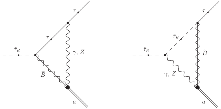
Figure 1: The dominant contributions to the two-body NLSP decay ${\widetilde{\tau}}_{\mathrm{R}}\to\tau+{\widetilde{a}}$.

Using the method described in Covi:2002vw , we obtain the following estimate for the decay rate:

$$\Gamma({\widetilde{\tau}}_{\mathrm{R}}\to\tau\,{\widetilde{a}}) = \frac{9\,\alpha^{4}\,C_{\rm aYY}^{2}}{512\pi^{5}\cos^{8}\theta_{W}}\,\,\frac{m_{{\widetilde{B}}}^{2}}{f_{a}^{2}}\,\,\frac{(m_{{\widetilde{\tau}}}^{2}-m_{{\widetilde{a}}}^{2})^{2}}{m_{{\widetilde{\tau}}}^{3}}\,\,\xi^{2}\,\log^{2}\left(\frac{f_{a}}{m}\right)$$ (2)

$$\simeq \xi^{2}\,(25~{}\mathrm{sec})^{-1}C_{\rm aYY}^{2}\left(1-\frac{m_{\widetilde{a}}^{2}}{m_{\widetilde{\tau}}^{2}}\right)\left(\frac{m_{{\widetilde{\tau}}}}{100\,\mbox{GeV}}\right)\left(\frac{10^{11}\,\mbox{GeV}}{f_{a}}\right)^{2}\left(\frac{m_{\tilde{B}}}{100\,\mbox{GeV}}\right)^{2},$$ (3)

where $m_{{\widetilde{B}}}$ is the mass of the bino and $m_{\widetilde{\tau}}$ is the mass of the stau NLSP, i.e. $m_{\widetilde{a}}<m_{\widetilde{\tau}}<m_{{\widetilde{B}}}$. As explained below, there is an uncertainty associated with the method used to derive the decay rate (2). We absorb this uncertainty into the mass scale $m\simeq m_{{\widetilde{\tau}},{\widetilde{B}}}\simeq{\cal O}(100\,\mbox{GeV})$ and into the factor $\xi\simeq{\cal O}(1)$ in the first line. We used $\log\left(f_{a}/m\right)\simeq 20.7$ to get from the first to the second line.

Here a technical comment on the loop integral is in order. If one naively integrates over the internal momentum in the diagrams with the effective vertex — see Fig. 1 — one encounters logarithmic divergencies. This is because the effective vertex (1) is applicable only if the momentum is smaller than the heavy (s)quark masses, whereas the momentum in the loop goes beyond that scale. In a rigorous treatment, one has to specify the origin of the effective vertex, i.e. the Peccei–Quinn sector, and to calculate the two-loop integrals with heavy (s)quarks in the additional loop. Such a two-loop computation leads to a finite result HSSW:2005 . Here, instead, we have regulated the logarithmic divergencies with the cut-off $f_{a}$ and kept only the dominant contribution. The mass scale $m$ and the factor $\xi$ have been introduced above to account for the uncertainty coming from this cut-off procedure.

II.3 The Three-Body Decay ${\widetilde{\tau}}\to\tau+\gamma+{\widetilde{a}}$

We now turn to the three-body decay ${\widetilde{\tau}}_{\mathrm{R}}\to\tau+\gamma+{\widetilde{a}}$. We again neglect the tau mass for simplicity. In contrast to the two-body decay considered above, the three-body decay occurs already at tree level, once the effective vertex given in (1) is used. In addition, we take into account photon radiation from the loop diagrams of Fig. 1, since the additional factor of $\alpha$ is partially compensated by the additional factor of $\log(f_{a}/m)$. As above, we keep only the dominant contribution of the loop diagrams. The corresponding Feynman diagrams are shown in Fig. 2,

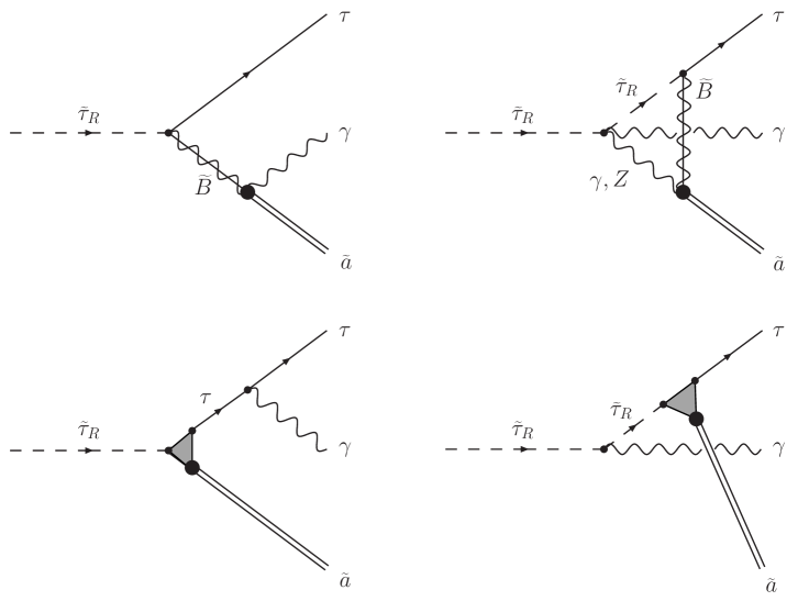
Figure 2: The dominant contributions to the three-body NLSP decay ${\widetilde{\tau}}_{\mathrm{R}}\to\tau+\gamma+{\widetilde{a}}$.

where a thick dot represents the effective vertex (1) and a shaded triangle the set of triangle diagrams given in Fig. 1. As the photon radiation from an electrically charged particle within the loops leads to a subdominant contribution, these processes are not shown in Fig. 2. At each order in $\log(f_{a}/m)$, only the leading order in $\alpha$ is computed while higher-order corrections are not considered. In terms of the observables that seem to be most accessible, i.e. the photon energy $E_{\gamma}$ and $\cos\theta$, the cosine of the opening angle between the photon and the tau direction, the corresponding differential decay rate reads

$$\frac{d^{2}\Gamma({\widetilde{\tau}}_{\mathrm{R}}\to\tau\,\gamma\,{\widetilde{a}})}{dx_{\gamma}\,d\cos\theta}=\frac{m_{{\widetilde{\tau}}}}{512\pi^{3}}\,\frac{x_{\gamma}(1-A_{\widetilde{a}}-x_{\gamma})}{[1-(x_{\gamma}/2)(1-\cos\theta)]^{2}}\,\sum_{\rm spins}|\mathcal{M}({\widetilde{\tau}}_{\mathrm{R}}\to\tau\,\gamma\,{\widetilde{a}})|^{2}\ ,$$ (4)

where

$$\sum_{\rm spins}|\mathcal{M}({\widetilde{\tau}}_{\mathrm{R}}\to\tau\,\gamma\,{\widetilde{a}})|^{2} = {\alpha^{3}\,\*C_{\rm aYY}^{2}\over\pi\*\cos^{4}\theta_{W}}\,\,\*{m_{{\widetilde{\tau}}}^{2}\over f_{a}^{2}}\*\,\,F_{\rm diff}^{({\widetilde{a}})}(x_{\gamma},\cos\theta,A_{\widetilde{a}},A_{\widetilde{B}})\ ,$$ (5)

with

$$x_{\gamma}\equiv\frac{2E_{\gamma}}{m_{{\widetilde{\tau}}}}\ ,\quad\quad A_{\widetilde{a}}\equiv\frac{m_{\widetilde{a}}^{2}}{m_{{\widetilde{\tau}}}^{2}}\ ,\quad\quad A_{\widetilde{B}}\equiv\frac{m_{\widetilde{B}}^{2}}{m_{{\widetilde{\tau}}}^{2}}\ ,$$ (6)

and

$$F_{\rm diff}^{({\widetilde{a}})}(x_{\gamma},\cos\theta,A_{\widetilde{a}},A_{\widetilde{B}})={x_{\gamma}^{2}\*(1\!-\!A_{\widetilde{a}}\!-\!x_{\gamma})\*[1\!+\!\cos\theta\!+\!A_{\widetilde{a}}\*(1\!-\!\cos\theta)]\*[1\!+\!\cos\theta\!+\!A_{\widetilde{B}}\*(1\!-\!\cos\theta)]\over\{x_{\gamma}\*(1+\cos\theta)+2\*A_{\widetilde{a}}-A_{\widetilde{B}}\*[2-x_{\gamma}(1-\cos\theta)]\}^{2}}$$

$$+\,\,{3\*\alpha\over\pi\*\cos^{2}\theta_{W}}\*\,\xi\*\log\left({f_{a}\over m}\right)\*\Bigg{\{}{\sqrt{A_{\widetilde{a}}\*A_{\widetilde{B}}}\*(1+\cos\theta)\*(1-A_{\widetilde{a}}-x_{\gamma})\over x_{\gamma}\*(1+\cos\theta)+2\*A_{\widetilde{a}}-A_{\widetilde{B}}\*[2-x_{\gamma}\*(1-\cos\theta)]}$$

$$\hskip 128.0374pt+\,{A_{\widetilde{B}}\*\left[(1+\cos\theta)\*(1-A_{\widetilde{a}})+A_{\widetilde{a}}\*x_{\gamma}\*(1-\cos\theta)\right]\over x_{\gamma}\*(1+\cos\theta)+2\*A_{\widetilde{a}}-A_{\widetilde{B}}\*[2-x_{\gamma}\*(1-\cos\theta)]}\Bigg{\}}$$

$$+\,\,{9\*\alpha^{2}\over 4\*\pi^{2}\*\cos^{4}\theta_{W}}\*\,\xi^{2}\*\log^{2}\left({f_{a}\over m}\right)\*A_{\widetilde{B}}\*\Bigg{\{}{1+\cos\theta+A_{\widetilde{a}}\*(1-\cos\theta)\over(1-\cos\theta)\*(1-A_{\widetilde{a}}-x_{\gamma})}+{2\*(1+\cos\theta)\*(1-A_{\widetilde{a}})\over x_{\gamma}^{2}\*(1-\cos\theta)}\Bigg{\}}\ .$$ (7)

Hereafter, we use $\log\left(f_{a}/m\right)\simeq 20.7$, as in the previous section.

The three-body decay ${\widetilde{\tau}}\to\tau+\gamma+{\widetilde{a}}$ involves bremsstrahlung processes (see Fig. 2) and, as already mentioned, we have neglected the tau mass. Thus, when the photon energy and/or the angle between the photon and the tau direction tend to zero, there are soft and/or collinear divergences. Consequently, the total rate of the decay ${\widetilde{\tau}}\to\tau+\gamma+{\widetilde{a}}$ is not defined. We define the integrated rate of the three-body decay ${\widetilde{\tau}}\to\tau+\gamma+{\widetilde{a}}$ with a cut on the scaled photon energy, $x_{\gamma}>x_{\gamma}^{\mathrm{cut}}$, and a cut on the cosine of the opening angle, $\cos\theta<1-x_{\theta}^{\mathrm{cut}}$:

$$\Gamma({\widetilde{\tau}}_{\mathrm{R}}\to\tau\,\gamma\,{\widetilde{a}}\,;x_{\gamma}^{\mathrm{cut}},x_{\theta}^{\mathrm{cut}})\equiv\int^{1-A_{\tilde{a}}}_{x_{\gamma}^{\mathrm{cut}}}dx_{\gamma}\int^{1-x_{\theta}^{\mathrm{cut}}}_{-1}d\cos\theta\frac{d^{2}\Gamma({\widetilde{\tau}}_{\mathrm{R}}\to\tau\,\gamma\,{\widetilde{a}})}{dx_{\gamma}d\cos\theta}\ .$$ (8)

As explained in Sec. IV, the quantity $\Gamma({\widetilde{\tau}}_{\mathrm{R}}\to\tau\,\gamma\,{\widetilde{a}}\,;x_{\gamma}^{\mathrm{cut}},x_{\theta}^{\mathrm{cut}})$ will be important in distinguishing between the axino LSP and the gravitino LSP scenarios.

II.4 Probing the Peccei–Quinn Scale and the Axino Mass

In the axino LSP scenario, the stau NLSP decays provide us with a new method to probe the Peccei–Quinn scale $f_{a}$ at colliders. As we will see in Sec. IV.2, the branching ratio of the three-body decay is small if reasonable cuts are used. Thus, we can use the two-body decay rate (3) to estimate the stau lifetime, $\tau_{\widetilde{\tau}}\approx 1/\Gamma({\widetilde{\tau}}\to\tau\,{\widetilde{a}})$. Accordingly, the Peccei–Quinn scale $f_{a}$ can be estimated as

$$f_{a}^{2}\simeq\left(\frac{\tau_{\widetilde{\tau}}}{25~{}\mathrm{sec}}\right)\,\xi^{2}\,C_{\rm aYY}^{2}\left(1-\frac{m_{\widetilde{a}}^{2}}{m_{\widetilde{\tau}}^{2}}\right)\left(\frac{m_{{\widetilde{\tau}}}}{100\,\mbox{GeV}}\right)\left(\frac{m_{\tilde{B}}}{100\,\mbox{GeV}}\right)^{2}\left(10^{11}\,\mbox{GeV}\right)^{2}\ ,$$ (9)

once $m_{\widetilde{\tau}}$, $m_{\widetilde{B}}$, and the lifetime of the stau $\tau_{\widetilde{\tau}}$ have been measured. The dependence on the axino mass is negligible for $m_{\widetilde{a}}/m_{\widetilde{\tau}}\buildrel<\over{{}_{\sim}}0.1$, so that $f_{a}$ can be determined without knowing $m_{\widetilde{a}}$. For larger values of $m_{\widetilde{a}}$, the stau NLSP decays can be used to determine the mass of the axino kinematically. In the two-body decay ${\widetilde{\tau}}\to\tau+{\widetilde{a}}$, the axino mass can be inferred from $E_{\tau}$, the energy of the emitted tau lepton:

$$m_{\widetilde{a}}=\sqrt{m_{\widetilde{\tau}}^{2}+m_{\tau}^{2}-2m_{\widetilde{\tau}}E_{\tau}}\ ,$$ (10)

with an error depending on the experimental uncertainty on $m_{\widetilde{\tau}}$ and $E_{\tau}$.

III Gravitino LSP Scenario

In this section we assume that the gravitino is the LSP and again that the pure right-handed stau is the NLSP. The corresponding rates of the two-body and three-body decay of the stau NLSP are given. These decays have already been studied in Refs. Buchmuller:2004rq . Here we generalize the result obtained for the three-body decay by taking into account finite values of the neutralino mass. For simplicity, we assume again that the lightest neutralino is a pure bino.

The couplings of the gravitino ${\widetilde{G}}$ to the ${\widetilde{\tau}}_{\mathrm{R}}$, $\tau$, ${\widetilde{B}}$, and $\gamma$ are given by the SUGRA Lagrangian Wess:1992cp . The interactions of the gravitino are determined uniquely by local SUSY and the Planck scale and, in constrast to the axino case, are not model-dependent.

III.1 The Two-Body Decay ${\widetilde{\tau}}\to\tau+{\widetilde{G}}$

In the gravitino LSP scenario, the main decay mode of the stau NLSP is the two-body decay ${\widetilde{\tau}}\to\tau+{\widetilde{G}}$. As there is a direct stau–tau–gravitino coupling, this process occurs at tree level. Neglecting the $\tau$-lepton mass $m_{\tau}$, one obtains the decay rate:

$$\Gamma({\widetilde{\tau}}_{\mathrm{R}}\to\tau\,{\widetilde{G}}) = \frac{m_{{\widetilde{\tau}}}^{5}}{48\pi\,m_{\widetilde{G}}^{2}\,\mathrm{M}_{\mathrm{Pl}}^{2}}\left(1-\frac{m_{\widetilde{G}}^{2}}{m_{{\widetilde{\tau}}}^{2}}\right)^{4}$$ (11)

$$= (5.89~{}\mathrm{sec})^{-1}\left(\frac{m_{{\widetilde{\tau}}}}{100~{}\mathrm{GeV}}\right)^{5}\left(\frac{10~{}\mathrm{MeV}}{m_{\widetilde{G}}}\right)^{2}\left(1-\frac{m_{\widetilde{G}}^{2}}{m_{{\widetilde{\tau}}}^{2}}\right)^{4}\ .$$ (12)

In order to get from the first to the second line, we have used the value of the reduced Planck mass $\mathrm{M}_{\mathrm{Pl}}=(8\pi\,G_{\rm N})^{-1/2}=2.435\times 10^{18}\,\mbox{GeV}$ as obtained from macroscopic measurements of Newton’s constant Eidelman:2004wy $G_{\rm N}=6.709\times 10^{-39}\,\mbox{GeV}^{-2}$. Thus, the gravitino mass can be determined once the stau NLSP lifetime governed by (12) and $m_{\widetilde{\tau}}$ are measured. As pointed out in Refs. Buchmuller:2004rq , expression (11) can also be used the other way around, i.e. for a microscopic determination of the Planck scale once the masses of the gravitino and the stau are measured kinematically. Note the strong dependence on $m_{\widetilde{G}}$ and $m_{\widetilde{\tau}}$. In the axino LSP scenario, the corresponding rate (2) becomes independent of the axino mass for $m_{{\widetilde{a}}}/m_{{\widetilde{\tau}}}\buildrel<\over{{}_{\sim}}0.1$, so that the Peccei–Quinn scale can be determined even if $m_{{\widetilde{a}}}$ is too small to be inferred kinematically.

III.2 The Three-Body Decay ${\widetilde{\tau}}\to\tau+\gamma+{\widetilde{G}}$

Let us now turn to the three-body decay ${\widetilde{\tau}}_{\mathrm{R}}\to\tau+\gamma+{\widetilde{G}}$. The corresponding Feynman diagrams are shown in Fig. 3.

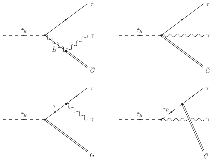
Figure 3: The three-body NLSP decay ${\widetilde{\tau}}_{\mathrm{R}}\to\tau+\gamma+{\widetilde{G}}$.

We neglect again the tau mass for simplicity. For finite bino mass, we obtain the following differential decay rate

$$\frac{d^{2}\Gamma({\widetilde{\tau}}_{\mathrm{R}}\to\tau\,\gamma\,{\widetilde{G}})}{dx_{\gamma}d\cos\theta}=\frac{m_{\tilde{\tau}}}{512\pi^{3}}\frac{x_{\gamma}(1-A_{{\widetilde{G}}}-x_{\gamma})}{[1-(x_{\gamma}/2)(1-\cos\theta)]^{2}}\sum_{\rm spins}|\mathcal{M}({\widetilde{\tau}}_{\mathrm{R}}\to\tau\,\gamma\,{\widetilde{G}})|^{2},$$ (13)

where

$$\sum_{\rm spins}|\mathcal{M}({\widetilde{\tau}}_{\mathrm{R}}\to\tau\,\gamma\,{\widetilde{G}})|^{2}=\frac{8\pi\alpha}{3}\,\,\frac{m_{\widetilde{\tau}}^{2}}{\mathrm{M}_{\mathrm{Pl}}^{2}\,A_{{\widetilde{G}}}}\,\,F_{\rm diff}^{({\widetilde{G}})}(x_{\gamma},\cos\theta,A_{{\widetilde{G}}},A_{\widetilde{B}})$$ (14)

with the definitions of $x_{\gamma}$ and $A_{\widetilde{B}}$ given in (6), $A_{\widetilde{G}}\equiv m_{\widetilde{G}}^{2}/m_{\widetilde{\tau}}^{2}$, and

$$F_{\rm diff}^{({\widetilde{G}})}(x_{\gamma},\cos\theta,A_{{\widetilde{G}}},A_{\widetilde{B}})=-3\*A_{{\widetilde{G}}}^{2}-7\*x_{\gamma}\*A_{{\widetilde{G}}}+{2\*(2-5\*\cos\theta)\*A_{{\widetilde{G}}}\over 1-\cos\theta}-{x_{\gamma}\*(1+\cos\theta)\over(1-\cos\theta)}$$

$$\quad-{(1+\cos\theta)\*(3+\cos\theta)\over(1-\cos\theta)^{2}}+{2\*(1-A_{{\widetilde{G}}})^{3}\*(1+\cos\theta)\over x_{\gamma}^{2}\*(1-\cos\theta)}+{A_{{\widetilde{G}}}\*(1-A_{{\widetilde{G}}})^{2}\over 1-A_{{\widetilde{G}}}-x_{\gamma}}$$

$$\quad+{(1-A_{{\widetilde{G}}})^{2}\*(1+\cos\theta)\over(1-A_{{\widetilde{G}}}-x_{\gamma})\*(1-\cos\theta)}-{4\*\left[1+\cos\theta+A_{{\widetilde{G}}}\*(1-\cos\theta)\right]^{2}\over\left[2-x_{\gamma}\*(1-\cos\theta)\right]^{2}\*(1-\cos\theta)^{2}}$$

$$\quad+{2\*\left\{3+\cos\theta\*\left[4-\cos\theta+2\*A_{{\widetilde{G}}}\*(1-\cos\theta)\right]\right\}\*\left[1+\cos\theta+A_{{\widetilde{G}}}\*(1-\cos\theta)\right]\over\left[2-x_{\gamma}\*(1-\cos\theta)\right]\*(1-\cos\theta)^{2}}$$

$$\quad+2\*(1-A_{{\widetilde{G}}}-x_{\gamma})\*\Bigg{\{}{1+x_{\gamma}-x_{\gamma}^{2}-2\*A_{{\widetilde{G}}}\*(1+3\*x_{\gamma}-2\*x_{\gamma}^{2})+A_{{\widetilde{G}}}^{2}\*(1+5\*x_{\gamma})\over x_{\gamma}\*(1-A_{\tilde{B}})\*(1-A_{{\widetilde{G}}}-x_{\gamma})}$$

$$\quad-{2\*\left[1+x_{\gamma}\*(2+A_{\tilde{B}})-x_{\gamma}^{2}+2\*A_{{\widetilde{G}}}\*(1-x_{\gamma})\right]\over x_{\gamma}\*\left[2-x_{\gamma}\*(1-\cos\theta)\right]}+{4\*(1-A_{{\widetilde{G}}}-x_{\gamma})\over\left[2-x_{\gamma}\*(1-\cos\theta)\right]^{2}}$$

$$\quad-{\sqrt{A_{{\widetilde{B}}}\*A_{{\widetilde{G}}}}\*\left[2\*(1+\cos\theta)\*(1-A_{{\widetilde{G}}})+3\*x_{\gamma}\*A_{{\widetilde{G}}}\*(1-\cos\theta)\right]\over x_{\gamma}\*(1+\cos\theta)+2\*(A_{{\widetilde{G}}}-A_{\tilde{B}})+A_{\tilde{B}}\*x_{\gamma}\*(1-\cos\theta)}$$

$$\quad-{2\*\left\{A_{{\widetilde{G}}}^{2}\*\left[-3-6\*x_{\gamma}+A_{\tilde{B}}\*(2+x_{\gamma})\right]+4\*A_{{\widetilde{B}}}\*A_{{\widetilde{G}}}\*(1+x_{\gamma}-x_{\gamma}^{2})\right\}\over x_{\gamma}\*(1-A_{\tilde{B}})\*\left[x_{\gamma}\*(1+\cos\theta)+2\*(A_{{\widetilde{G}}}-A_{\tilde{B}})+A_{\tilde{B}}\*x_{\gamma}\*(1-\cos\theta)\right]}$$

$$\quad+{2\*A_{\tilde{B}}^{2}\*\left[(1-x_{\gamma})\*(1+2\*A_{{\widetilde{G}}}+x_{\gamma})+x_{\gamma}\*A_{\tilde{B}}\right]\over x_{\gamma}\*(1-A_{\tilde{B}})\*\left[x_{\gamma}\*(1+\cos\theta)+2\*(A_{{\widetilde{G}}}-A_{\tilde{B}})+A_{\tilde{B}}\*x_{\gamma}\*(1-\cos\theta)\right]}\Bigg{\}}$$

$$\quad+(1-A_{{\widetilde{G}}}-x_{\gamma})\*\Bigg{\{}{(-1+3\*A_{{\widetilde{G}}})\*(1-A_{{\widetilde{G}}})\over(1-A_{\tilde{B}})}+{2\*\left[2-x_{\gamma}-2\*(A_{{\widetilde{G}}}-A_{\tilde{B}})\right]\over 2-x_{\gamma}\*(1-\cos\theta)}$$

$$\quad-{4\*(1-A_{{\widetilde{G}}}-x_{\gamma})\over\left[2-x_{\gamma}\*(1-\cos\theta)\right]^{2}}-{2\*(A_{{\widetilde{G}}}-A_{\tilde{B}})\*\left[3\*A_{{\widetilde{G}}}\*(2-2\*A_{{\widetilde{G}}}-x_{\gamma})+A_{\tilde{B}}\*(2-2\*A_{\tilde{B}}+x_{\gamma})\right]\over(1-A_{\tilde{B}})\*\left[x_{\gamma}\*(1+\cos\theta)+2\*(A_{{\widetilde{G}}}-A_{\tilde{B}})+A_{\tilde{B}}\*x_{\gamma}\*(1-\cos\theta)\right]}$$

$$\quad+{4\*(1-A_{{\widetilde{G}}}-x_{\gamma})\*(3\*A_{{\widetilde{G}}}+A_{\tilde{B}})\*(A_{{\widetilde{G}}}-A_{\tilde{B}})^{2}\over(1-A_{\tilde{B}})\*\left[x_{\gamma}\*(1+\cos\theta)+2\*(A_{{\widetilde{G}}}-A_{\tilde{B}})+A_{\tilde{B}}\*x_{\gamma}\*(1-\cos\theta)\right]^{2}}\Bigg{\}}\ .$$ (15)

In the limit $m_{{\widetilde{B}}}\to\infty$, only the terms in the first four lines of (15) remain and the result given in the appendix of the first reference in Buchmuller:2004rq is obtained. For finite values of the bino mass, the diagram with the bino propagator in Fig. 3 has to be taken into account, which then leads to our more general result.

As in the axino case, the total rate of the three-body decay ${\widetilde{\tau}}\to\tau+\gamma+{\widetilde{G}}$ is not defined. We thus introduce again the integrated rate with a cut on the scaled photon energy, $x_{\gamma}>x_{\gamma}^{\mathrm{cut}}$, and a cut on the cosine of the opening angle, $\cos\theta<1-x_{\theta}^{\mathrm{cut}}$,

$$\Gamma({\widetilde{\tau}}_{\mathrm{R}}\to\tau\,\gamma\,{\widetilde{G}}\,;x_{\gamma}^{\mathrm{cut}},x_{\theta}^{\mathrm{cut}}) = \int^{1-A_{\tilde{G}}}_{x_{\gamma}^{\mathrm{cut}}}dx_{\gamma}\int^{1-x_{\theta}^{\mathrm{cut}}}_{-1}d\cos\theta\frac{d^{2}\Gamma({\widetilde{\tau}}_{\mathrm{R}}\to\tau\,\gamma\,{\widetilde{G}})}{dx_{\gamma}d\cos\theta}\ .$$ (16)

This quantity will be used in our comparison of collider signatures of the axino LSP and the gravitino LSP scenarios.

IV Axino vs. Gravitino

In this section we show how the two-body and three-body decays of the stau NLSP can be used to distinguish between the axino LSP scenario and the gravitino LSP scenario at colliders. We compare the total decay rates of the stau NLSP, the branching ratios of the three-body decays ${\widetilde{\tau}}\to\tau+\gamma+{\widetilde{a}}/{\widetilde{G}}$ with cuts on the observables, and the differential distributions of the decay products in the three-body decays.

IV.1 Total Decay Rates

Let us discuss the lifetime of the stau NLSP in the axino LSP and in the gravitino LSP scenarios, and examine whether the lifetime can be used to distinguish between the two. In both cases, the total decay rate of the stau NLSP is dominated by the two-body decay,

$$\Gamma^{\rm{total}}_{\tilde{\tau}_{R}\,\to\,i\,X}\simeq\Gamma({\widetilde{\tau}}_{\mathrm{R}}\to\tau\,i)\ ,\quad i={\widetilde{a}},{\widetilde{G}}\ ,$$ (17)

with the rates given respectively in (3) and (12). Thus, the order of magnitude of the stau NLSP lifetime is (essentially) determined by $m_{\widetilde{\tau}}$, $m_{\widetilde{B}}$, and $f_{a}$ in the axino LSP scenario and by $m_{\widetilde{\tau}}$ and $m_{\widetilde{G}}$ in the gravitino LSP scenario. Among those parameters, one should be able to measure the stau mass $m_{\widetilde{\tau}}$ and the bino mass $m_{\widetilde{B}}$ by analysing the other processes occurring in the planned collider detectors. Indeed, we expect that these masses will already be known when the stau NLSP decays are analysed. To be specific, we set these masses to $m_{\widetilde{\tau}}=100\,\mbox{GeV}$ and $m_{\widetilde{B}}=110\,\mbox{GeV}$, keeping in mind the NLSP lifetime dependencies $\tau_{\widetilde{\tau}}\propto 1/(m_{\widetilde{\tau}}\,m_{\widetilde{B}}^{2})$ for the axino LSP and $\tau_{\widetilde{\tau}}\propto 1/m_{\widetilde{\tau}}^{5}$ for the gravitino LSP. Then, the order of magnitude of the stau NLSP lifetime is governed by the Peccei–Quinn scale $f_{a}$ in the axino LSP scenario and by the gravitino mass $m_{\widetilde{G}}$ in the gravitino LSP scenario.

In the axino LSP scenario, the stau lifetime varies from ${\cal O}(0.01~{}{\mbox{sec}})$ to ${\cal O}(10~{}{\mbox{h}})$ if we change the Peccei–Quinn scale $f_{a}$ from $5\times 10^{9}\,\mbox{GeV}$ to $5\times 10^{12}\,\mbox{GeV}$, as can be seen from (3). For the given values of $m_{\widetilde{\tau}}$ and $m_{\widetilde{B}}$, these values can probably be considered as the lower and upper bounds on the stau NLSP lifetime in the axino LSP case.

In the gravitino LSP case, the stau lifetime can vary over a much wider range, e.g. from $6\times 10^{-8}\,{\rm sec}$ to 15 years by changing the gravitino mass $m_{\widetilde{G}}$ from 1 keV to 50 GeV, as can be seen from (12). Therefore, both a very short stau NLSP lifetime, $\tau_{\widetilde{\tau}}\buildrel<\over{{}_{\sim}}$ msec, and a very long one, $\tau_{\widetilde{\tau}}\buildrel>\over{{}_{\sim}}$ days, will point to the gravitino LSP scenario. For example, in gravity-mediated SUSY breaking models, the gravitino mass is typically $(10$–$100)\,\mbox{GeV}$. Then, the lifetime of the NLSP becomes of ${\cal O}(\mbox{years})$ and points clearly to the gravitino LSP scenario.

On the other hand, if the observed lifetime of the stau NLSP is within the range ${\cal O}(0.01~{}{\mbox{sec}})$–${\cal O}(10~{}{\mbox{h}})$, it will be very difficult to distinguish between the axino LSP and the gravitino LSP scenarios from the stau NLSP lifetime alone. In this case, the analysis of the three-body NLSP decays will be crucial to distinguish between the two scenarios.

IV.2 Branching Ratio of the Three-Body Decay Modes

We now consider the branching ratio of the integrated rate of the three-body decay ${\widetilde{\tau}}\to\tau+\gamma+{\widetilde{a}}/{\widetilde{G}}$ with cuts

$$BR({\widetilde{\tau}}_{\mathrm{R}}\to\tau\,\gamma\,i\,;x_{\gamma}^{\mathrm{cut}},x_{\theta}^{\mathrm{cut}})\equiv{\Gamma({\widetilde{\tau}}_{\mathrm{R}}\to\tau\,\gamma\,i\,;x_{\gamma}^{\mathrm{cut}},x_{\theta}^{\mathrm{cut}})\over\Gamma^{\rm{total}}_{\tilde{\tau}_{R}\,\to\,i\,X}}\ ,\quad i={\widetilde{a}},{\widetilde{G}}\ .$$ (18)

In Fig. 4

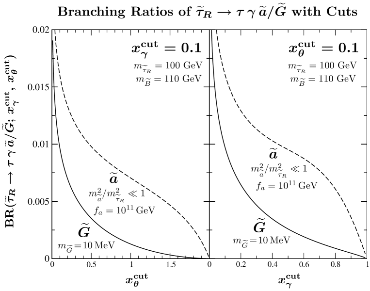
Figure 4: The branching ratio of the integrated rate of the three-body decay ${\widetilde{\tau}}\to\tau+\gamma+{\widetilde{a}}/{\widetilde{G}}$ with cuts as a function of $x_{\theta}^{\mathrm{cut}}$ for $x_{\gamma}^{\rm cut}=0.1$ (left) and as a function of $x_{\gamma}^{\mathrm{cut}}$ for $x_{\theta}^{\mathrm{cut}}=0.1$ (right). The solid and dashed lines show the results for the gravitino LSP and the axino LSP, respectively, as obtained with $m_{\widetilde{\tau}}=100\,\mbox{GeV}$, $m_{\widetilde{B}}=110\,\mbox{GeV}$, $f_{a}=10^{11}\,\mbox{GeV}$, $\xi^{2}C_{\rm aYY}^{2}=1$, $m_{{\widetilde{a}}}^{2}/m_{{\widetilde{\tau}}}^{2}\ll 1$, and $m_{\widetilde{G}}=10\,\mbox{MeV}$.

this quantity is shown for the gravitino LSP (solid line) and the axino LSP (dashed line) for $m_{\widetilde{\tau}}=100\,\mbox{GeV}$, $m_{\widetilde{B}}=110\,\mbox{GeV}$, $f_{a}=10^{11}\,\mbox{GeV}$, $\xi^{2}C_{\rm aYY}^{2}=1$, $m_{{\widetilde{a}}}^{2}/m_{{\widetilde{\tau}}}^{2}\ll 1$, and $m_{\widetilde{G}}=10\,\mbox{MeV}$. In the left (right) part of the figure we fix $x_{\gamma}^{\mathrm{cut}}=0.1$ ($x_{\theta}^{\mathrm{cut}}=0.1$) and vary $x_{\theta}^{\mathrm{cut}}$ ($x_{\gamma}^{\mathrm{cut}}$). The dependence of the branching ratio (18) on the cut parameters in the axino LSP case differs qualitatively from the one in the gravitino LSP case. Moreover, there is a significant excess of $BR({\widetilde{\tau}}_{\mathrm{R}}\to\tau\,\gamma\,{\widetilde{a}}\,;x_{\gamma}^{\mathrm{cut}},x_{\theta}^{\mathrm{cut}})$ over $BR({\widetilde{\tau}}_{\mathrm{R}}\to\tau\,\gamma\,{\widetilde{G}}\,;x_{\gamma}^{\mathrm{cut}},x_{\theta}^{\mathrm{cut}})$ over large ranges in the cut parameters. For example, if $10^{4}$ stau NLSP decays can be analysed and the cuts are set to $x_{\gamma}^{\mathrm{cut}}=x_{\theta}^{\mathrm{cut}}=0.1$, we expect about 165$\pm$13 (stat.) ${\widetilde{\tau}}_{\mathrm{R}}\to\tau\,\gamma\,{\widetilde{a}}$ events for the axino LSP and about 100$\pm$10 (stat.) ${\widetilde{\tau}}_{\mathrm{R}}\to\tau\,\gamma\,{\widetilde{G}}$ events for the gravitino LSP. Thus, the measurement of the branching ratio (18) would allow a distinction to be made between the axino LSP and the gravitino LSP scenarios. For a smaller number of analysed stau NLSP decays, this distinction becomes more difficult. In addition to the statistical errors, details of the detectors and of the additional massive material needed to stop the staus and to analyse their decays will be important to judge on the feasibility of the distinction based on the branching ratios. We postpone this study for future work.

IV.3 Differential Distributions in the Three-Body Decays

Finally, we consider the differential distributions of the visible decay products in the three-body decays ${\widetilde{\tau}}\to\tau+\gamma+{\widetilde{a}}/{\widetilde{G}}$ in terms of the quantity

$${1\over\Gamma({\widetilde{\tau}}_{\mathrm{R}}\to\tau\,\gamma\,i\,;x_{\gamma}^{\mathrm{cut}},x_{\theta}^{\mathrm{cut}})}\,\,{d^{2}\Gamma({\widetilde{\tau}}_{\mathrm{R}}\to\tau\,\gamma\,i)\over dx_{\gamma}d\cos\theta}\ ,\quad i={\widetilde{a}},{\widetilde{G}}\ ,$$ (19)

which is independent of the two-body decay, the total NLSP decay rate, and the Peccei–Quinn/Planck scale. In Fig. 5,

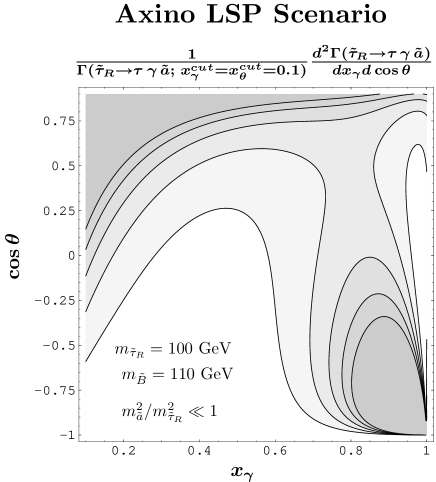
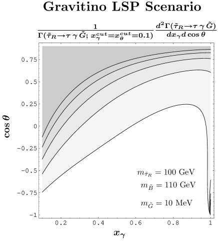
Figure 5: The normalized differential distributions of the visible decay products in the decays ${\widetilde{\tau}}\to\tau+\gamma+{\widetilde{a}}/{\widetilde{G}}$ for the axino LSP scenario (left) and the gravitino LSP scenario (right) for $m_{\widetilde{\tau}}=100\,\mbox{GeV}$, $m_{\widetilde{B}}=110\,\mbox{GeV}$, $m_{{\widetilde{a}}}^{2}/m_{{\widetilde{\tau}}}^{2}\ll 1$, and $m_{\widetilde{G}}=10\,\mbox{MeV}$. The cut parameters are set to $x_{\gamma}^{\mathrm{cut}}=x_{\theta}^{\mathrm{cut}}=0.1$. The contour lines represent the values 0.2, 0.4, 0.6, 0.8, and 1.0, where the darker shading implies a higher number of events.

the normalized differential distributions (19) with $x_{\gamma}^{\mathrm{cut}}=x_{\theta}^{\mathrm{cut}}=0.1$ are shown for the axino LSP scenario (left) and the gravitino LSP scenario (right) for $m_{\widetilde{\tau}}=100\,\mbox{GeV}$, $m_{\widetilde{B}}=110\,\mbox{GeV}$, $m_{{\widetilde{a}}}^{2}/m_{{\widetilde{\tau}}}^{2}\ll 1$, and $m_{\widetilde{G}}=10\,\mbox{MeV}$. In the case of the gravitino LSP, the events are peaked only in the region where the photons are soft and the photon and the tau are emitted with a small opening angle ($\theta\simeq 0$). In contrast, in the axino LSP scenario, the events are also peaked in the region where the photon energy is large and the photon and the tau are emitted back-to-back ($\theta\simeq\pi$). Thus, if the observed number of events peaks in both regions, there is strong evidence for the axino LSP and against the gravitino LSP.

To be specific, with $10^{4}$ analysed stau NLSP decays, we expect about 165$\pm$13 (stat.) events for the axino LSP and about 100$\pm$10 (stat.) events for the gravitino LSP, which will be distributed over the corresponding ($x_{\gamma}$, $\cos\theta$)-planes shown in Fig. 5. In particular, in the region of $x_{\gamma}\gtrsim 0.8$ and $\cos\theta\lesssim-0.3$, we expect about 28% of the 165$\pm$13 (stat.) events in the axino LSP case and about 1% of the 100$\pm$10 (stat.) events in the gravitino LSP case. These numbers illustrate that ${\cal O}(10^{4})$ of analysed stau NLSP decays could be sufficient for the distinction based on the differential distributions. To establish the feasibility of this distinction, a dedicated study taking into account the details of the detectors and the additional massive material will be crucial, which we leave for future studies.

Some comments are in order. The differences between the two scenarios shown in Figs. 4 and 5 become smaller for larger values of $m_{\widetilde{B}}/m_{\widetilde{\tau}}$. This ratio, however, remains close to unity for the stau NLSP in unified models. Furthermore, if $m_{\widetilde{G}}<m_{{\widetilde{a}}}<m_{\mathrm{LOSP}}$ — mentioned as case (iv) in the Introduction — and $\Gamma({\widetilde{\tau}}\to{\widetilde{a}}\,X)\gg\Gamma({\widetilde{\tau}}\to{\widetilde{G}}\,X)$, one would still find the distribution shown in the left panel of Fig. 5. The axino would then eventually decay into the gravitino LSP and the axion. Conversely, the distribution shown in the right panel of Fig. 5 would be obtained if $m_{{\widetilde{a}}}<m_{\widetilde{G}}<m_{\mathrm{LOSP}}$ — mentioned as case (iii) in the Introduction — and $\Gamma({\widetilde{\tau}}\to{\widetilde{a}}\,X)\ll\Gamma({\widetilde{\tau}}\to{\widetilde{G}}\,X)$. Then it would be the gravitino that would eventually decay into the axino LSP and the axion. Barring these caveats, the signatures shown in Figs. 4 and 5 will provide a clear distinction between the axino LSP and the gravitino LSP scenarios.

V Conclusion

Assuming that a charged slepton is the NLSP, we have discussed signatures of both the gravitino LSP scenario and the axino LSP scenario in the framework of hadronic, or KSVZ, axion models Kim:1979if+X . These signatures can be observed at future colliders if the planned detectors are equipped with 1–10 kt of additional material to stop and collect charged NLSPs Hamaguchi:2004df ; Feng:2004yi . With calorimetric and tracking performance, this additional material will serve simultaneously as a real-time detector, allowing an analysis of the decays of the trapped NLSPs with high efficiency Hamaguchi:2004df .

In the scenario in which the axino is the LSP, we have shown that the NLSP lifetime can be used to estimate the Peccei–Quinn scale $f_{a}$. Indeed, if the axino is the LSP, the NLSP decays provide us with a new way to probe the Peccei–Quinn sector. This method is complementary to the existing and planned axion search experiments. The decays of the NLSP into the axino LSP will also allow us to determine the axino mass kinematically if it is not much smaller than the mass of the NLSP. The determination of both the Peccei–Quinn scale $f_{a}$ and the axino mass $m_{\widetilde{a}}$ will be crucial for insights into the cosmological relevance of the axino LSP. Once $f_{a}$ and $m_{\widetilde{a}}$ are known, we will be able to decide if axinos are present as cold dark matter in our Universe.

In the gravitino LSP scenario, the measurement of the stau NLSP lifetime can be used to determine the gravitino mass $m_{\widetilde{G}}$ once the mass of the NLSP is known. This will be crucial for insights into the SUSY breaking mechanism. Moreover, if the gravitino mass can be determined independently from the kinematics and if the NLSP mass is known, the NSLP lifetime provides a microscopic measurement of the Planck scale Buchmuller:2004rq . Indeed, if the gravitino is the LSP, the lifetime of the NLSP depends strongly on the Planck scale and the masses of the NLSP and the gravitino.

We have addressed the question of how to distinguish between the axino LSP and the gravitino LSP scenarios at colliders. If the mass of the LSP cannot be measured and if the NLSP lifetime is within the range ${\cal O}(0.01~{}{\mbox{sec}})$–${\cal O}(10~{}{\mbox{h}})$, we have found that the NLSP lifetime alone will not allow us to distinguish clearly between the axino LSP and the gravitino LSP scenarios. The situation is considerably improved when one considers the three-body decay of a charged slepton NLSP into the associated charged lepton, a photon, and the LSP. We have found qualitative and quantitative differences between the branching ratios of the integrated three-body decay rate with cuts on the photon energy and the angle between the lepton and photon directions. In addition, the differential distributions of the decay products in the three-body decays provide characteristic fingerprints. For a clear distinction between the axino LSP and the gravitino LSP scenarios based on the three-body decay events, at least of ${\cal O}(10^{4})$ of analysed stau NLSP decays are needed. If the mass of the stau NLSP is not significantly larger than 100 GeV, this number could be obtained at both the LHC and the ILC with 1–10 kt of massive additional material around the main detectors.

References

-
(1)
H. P. Nilles,
Phys. Rep. 110 (1984) 1;
H. E. Haber and G. L. Kane, Phys. Rep. 117 (1985) 75;
S. P. Martin, hep-ph/9709356. -
(2)
L. Covi, J. E. Kim and L. Roszkowski,
Phys. Rev. Lett. 82 (1999) 4180
[hep-ph/9905212];
L. Covi, H. B. Kim, J. E. Kim and L. Roszkowski, JHEP 0105 (2001) 033 [hep-ph/0101009]. -
(3)
A. Brandenburg and F. D. Steffen,
JCAP 0408 (2004) 008
[hep-ph/0405158];
hep-ph/0406021; hep-ph/0407324. - (4) T. Moroi, H. Murayama and M. Yamaguchi, Phys. Lett. B 303 (1993) 289.
-
(5)
M. Bolz, W. Buchmüller and M. Plümacher,
Phys. Lett. B 443 (1998) 209
[hep-ph/9809381];
M. Bolz, A. Brandenburg and W. Buchmüller, Nucl. Phys. B 606 (2001) 518 [hep-ph/0012052]. -
(6)
M. Fujii and T. Yanagida,
Phys. Lett. B 549 (2002) 273
[hep-ph/0208191];
W. Buchmüller, K. Hamaguchi and M. Ratz, Phys. Lett. B 574 (2003) 156 [hep-ph/0307181];
M. Fujii, M. Ibe and T. Yanagida, Phys. Rev. D 69 (2004) 015006 [hep-ph/0309064];
M. Ibe and T. Yanagida, Phys. Lett. B 597 (2004) 47 [hep-ph/0404134]. -
(7)
J. L. Feng, A. Rajaraman and F. Takayama,
Phys. Rev. Lett. 91 (2003) 011302
[hep-ph/0302215];
Phys. Rev. D 68 (2003) 063504
[hep-ph/0306024];
J. L. Feng, S. Su and F. Takayama, Phys. Rev. D 70 (2004) 063514 [hep-ph/0404198]. - (8) L. Roszkowski and R. Ruiz de Austri, hep-ph/0408227.
-
(9)
H. P. Nilles and S. Raby,
Nucl. Phys. B 198 (1982) 102;
J. E. Kim and H. P. Nilles, Phys. Lett. B 138 (1984) 150. - (10) K. Tamvakis and D. Wyler, Phys. Lett. B 112 (1982) 451.
- (11) J. E. Kim, Phys. Lett. B 136 (1984) 378.
- (12) R. D. Peccei and H. R. Quinn, Phys. Rev. Lett. 38 (1977) 1440; Phys. Rev. D 16 (1977) 1791.
- (13) J. F. Nieves, Phys. Rev. D 33 (1986) 1762.
- (14) K. Rajagopal, M. S. Turner and F. Wilczek, Nucl. Phys. B 358 (1991) 447.
-
(15)
T. Goto and M. Yamaguchi,
Phys. Lett. B 276 (1992) 103;
E. J. Chun, J. E. Kim and H. P. Nilles, Phys. Lett. B 287 (1992) 123 [hep-ph/9205229];
E. J. Chun and A. Lukas, Phys. Lett. B 357 (1995) 43 [hep-ph/9503233]. - (16) J. Wess and J. Bagger, Supersymmetry and supergravity (Princeton University Press, Princeton, 1992).
-
(17)
M. Dine, A. E. Nelson and Y. Shirman,
Phys. Rev. D 51 (1995) 1362
[hep-ph/9408384];
M. Dine, A. E. Nelson, Y. Nir and Y. Shirman, Phys. Rev. D 53 (1996) 2658 [hep-ph/9507378];
G. F. Giudice and R. Rattazzi, Phys. Rep. 322 (1999) 419 [hep-ph/9801271]. -
(18)
L. Randall and R. Sundrum,
Nucl. Phys. B 557 (1999) 79
[hep-th/9810155];
G. F. Giudice, M. A. Luty, H. Murayama and R. Rattazzi, JHEP 9812 (1998) 027 [hep-ph/9810442]. - (19) P. Sikivie, Nucl. Phys. Proc. Suppl. 87 (2000) 41 [hep-ph/0002154].
- (20) S. Eidelman et al. [Particle Data Group], Phys. Lett. B 592 (2004) 1.
- (21) L. Covi, L. Roszkowski, R. Ruiz de Austri and M. Small, JHEP 0406 (2004) 003 [hep-ph/0402240].
-
(22)
M. Fujii, M. Ibe and T. Yanagida,
Phys. Lett. B 579 (2004) 6
[hep-ph/0310142];
J. R. Ellis, K. A. Olive, Y. Santoso and V. C. Spanos, Phys. Lett. B 588 (2004) 7 [hep-ph/0312262];
J. L. Feng, S. Su and F. Takayama, Phys. Rev. D 70 (2004) 075019 [hep-ph/0404231]. - (23) K. Hamaguchi, Y. Kuno, T. Nakaya and M. M. Nojiri, Phys. Rev. D 70 (2004) 115007 [hep-ph/0409248].
- (24) J. L. Feng and B. T. Smith, Phys. Rev. D 71 (2005) 015004 [hep-ph/0409278].
- (25) W. Buchmüller, K. Hamaguchi, M. Ratz and T. Yanagida, Phys. Lett. B 588 (2004) 90 [hep-ph/0402179]; hep-ph/0403203.
-
(26)
J. E. Kim,
Phys. Rev. Lett. 43 (1979) 103;
M. A. Shifman, A. I. Vainshtein and V. I. Zakharov, Nucl. Phys. B 166 (1980) 493. -
(27)
M. Dine, W. Fischler and M. Srednicki,
Phys. Lett. B 104 (1981) 199;
A. R. Zhitnitsky, Sov. J. Nucl. Phys. 31 (1980) 260. - (28) L. Covi, L. Roszkowski and M. Small, JHEP 0207 (2002) 023 [hep-ph/0206119].
- (29) S. Schilling, F. D. Steffen and D. Wyler, in preparation.