Next-to-leading order QCD predictions for pair production of neutral Higgs bosons at the CERN Large Hadron Collider

Abstract

We present the calculations of the complete NLO inclusive total cross sections for pair production of neutral Higgs bosons through $b\bar{b}$ annihilation in the minimal supersymmetric standard model at the CERN Large Hadron Collider. In our calculations, we used both the DREG scheme and the DRED scheme and found that the NLO total cross sections in these two schemes are the same. Our results show that the $b\bar{b}$-annihilation contributions can exceed those of $gg$ fusion and $q\bar{q}$ annihilation for $h^{0}H^{0}$, $A^{0}h^{0}$ and $A^{0}H^{0}$ productions when $\tan\beta$ is large. In the case of $\mu>0$, the NLO corrections enhance the LO total cross sections significantly, reaching a few tens of percent, while for $\mu<0$, the corrections are relatively small, and are negative in most of parameter space. Moreover, the NLO QCD corrections reduce the dependence of the total cross sections on the renormalization/factorization scale, especially for $\mu<0$. We also used the CTEQ6.1 PDF sets to estimate the uncertainty of LO and NLO total cross sections, and found that the uncertainty arising from the choice of PDFs increases with the increasing $m_{A^{0}}$.

I Introduction

The Higgs mechanism plays a key role for spontaneous breaking of the electroweak symmetry both in the standard model (SM) and in the minimal supersymmetric (MSSM) extension of the SM nilles . Therefore, the search for Higgs bosons becomes one of the prime tasks in future high-energy experiments, especially at the CERN Large Hadron Collider (LHC), with $\sqrt{S}=14$ TeV and a luminosity of 100 ${\rm fb^{-1}}$ per year lhc . In the SM, only one Higgs doublet is introduced, and the neutral CP-even Higgs boson mass is basically a free parameter with a theoretical upper bound of $m_{H}\leq 600$ – 800 GeV massh and a LEP2 experimental lower bound of $m_{H}\geq 114.4$ GeV parameter . In the MSSM, two Higgs doublets are required in order to preserve supersymmetry (SUSY), and consequently the model predicts five physical Higgs bosons: the neutral CP-even ones $h^{0}$ and $H^{0}$, the neutral CP-odd one $A^{0}$, and the charged ones $H^{\pm}$. The $h^{0}$, which behaves like the SM one in the decoupling region ($m_{A^{0}}\gg m_{Z^{0}}$), is the lightest, and its mass is constrained by a theoretical upper bound of $m_{h^{0}}\leq 140$ GeV when including the radiative corrections massh0 . The analyses in detect indicate that the $h^{0}$ boson can not escape detection at the LHC, and that in large areas of the parameter space, more than one Higgs particle in the MSSM can possibly be found, which is an exciting result, since the discovery of any additional Higgs bosons will be direct evidence of physics beyond the SM.

At the LHC, a neutral Higgs boson $\phi$ can be produced through following mechanisms: gluon fusion $gg\rightarrow\phi$ gg2h , weak boson fusion $qq\rightarrow qqV^{*}V^{*}\rightarrow qqh^{0}/qqH^{0}$ vv2h , associated production with weak bosons v2vh , pair production hpair0 ; hpair1 ; hpair11 ; hpair2 , and associated production with a $t\bar{t}$ pair $gg/q\bar{q}\rightarrow t\bar{t}\phi$ ttbbh . In the MSSM, since the couplings between Higgs bosons and $b$ quarks can be enhanced by large values of $\tan\beta$, the ratio of the vacuum expectation values of the two Higgs doublets, Higgs bosons will also be copiously produced in association with $b$ quarks at the LHC. Except for $q\bar{q}\rightarrow b\bar{b}h^{0}$, the other relevant production mechanisms depend on the final state being observed differenth . For inclusive Higgs production, the lowest order process is $b\bar{b}\rightarrow h^{0}$ bbh , and the convergence of the perturbative expansion is improved by summing the collinear logarithms to all orders through the use of $b$ quark parton distributions with an appropriate factorization scale. However, if at least one high-$p_{T}$ $b$ quark is required to be observed, the leading partonic process is $gb\rightarrow bh^{0}$ gbbh , and if two high-$p_{T}$ $b$ quarks are required, the leading subprocess is $gg\rightarrow b\bar{b}h^{0}$ ggbbh .

Studying the pair production of neutral Higgs bosons may be an important way to probe the trilinear neutral Higgs boson couplings, which can distinguish between the SM and the MSSM. In the SM, Higgs boson pair production is dominated by $gg$ fusion mediated via heavy-quark loops, while the contribution of $q\bar{q}$ annihilation is greatly suppressed by the absence of the $HHZ$ coupling and the smallness of the $Hq\bar{q}$ ($q=u,d,s,c,b$) couplings. In the MSSM, $gg$ fusion for the pair production of neutral Higgs bosons can be mediated via both quark loops hpair0 ; hpair1 and squark loops hpair11 ; hpair2 , and the existence of $h^{0}A^{0}Z$ and $H^{0}A^{0}Z$ couplings at the tree level leads to $h^{0}A^{0}$ and $H^{0}A^{0}$ associated productions through $q\bar{q}$ annihilations (Drell-Yan-like processes) hpair0 . Moreover, since the $\phi b\bar{b}$ couplings can be greatly enhanced by large values of $\tan\beta$, there are potentially important contributions arising from $b\bar{b}$ annihilation to pair production of neutral Higgs bosons, which have been studied at the leading-order (LO) hpair2 . However, the LO predictions generally have a large uncertainty due to scale and PDF choices. In this paper, we present the complete next-to-leading order (NLO) QCD (including SUSY-QCD) calculation for the cross sections for pair production of neutral Higgs boson through $b\bar{b}$ annihilation at the LHC. Similar to single Higgs boson production, for the inclusive production the use of $b$ quark parton distributions at the LO will improve the convergence of the perturbative expansion. For simplicity, we neglect the bottom quark mass except in the Yukawa couplings, which is valid in all diagrams where the bottom quark is an initial state parton, according to the simplified Aivazis-Collins-Olness-Tung (ACOT) scheme acot . For regularization of the ultraviolet (UV), soft and collinear divergences, both the dimensional regularization (DREG) approach DREG (with naive $\gamma_{5}$ gamma5 ) and the dimensional reduction (DRED) scheme DRED are used in our calculations providing a cross check.

This paper is organized as follows. In Sect.II we show the analytic results for the LO cross sections proceeding through $b\bar{b}$ annihilation. In Sect.III we present the details of the calculations of both the virtual and real parts of the NLO QCD corrections, and compare the results using DREG with those using DRED. In Sect.IV we give the numerical predictions for inclusive and differential cross sections at the LHC. The relevant coupling constants and the lengthy analytic expressions are summarized in Appendices A, B and C.

II Leading Order Pair Production of Neutral Higgs Bosons

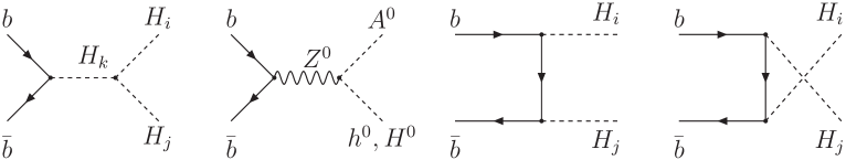
Figure 1: Leading order Feynman diagrams for $b\bar{b}\rightarrow H_{i}H_{j}$.

The tree-level Feynman diagrams for the subprocess $b(p_{a})\bar{b}(p_{b})\rightarrow H_{i}(p_{1})H_{j}(p_{2})$, where $H_{i=1,2,3}=H^{0},h^{0},A^{0}$, are shown in Fig. 1, and its LO amplitude in $n=4-2\epsilon$ dimensions is

$$M^{B}_{ij}=\mu_{r}^{2\epsilon}[M_{ij}^{(s)}+M_{ij}^{(t)}+M_{ij}^{(u)}],$$ (1)

with

$$M_{ij}^{(s)}=-\sum_{k=1}^{4}\frac{ig^{2}Y_{b}m_{Z}C_{kij}}{2c_{W}s_{H_{k}}}\bar{v}(p_{b})(a_{k}P_{L}+a_{k}^{\ast}P_{R})u(p_{a})$$

$$\hskip 39.83368pt-\frac{\delta_{i3}g^{2}Z_{j}^{H}}{2c_{W}^{2}(s-m_{Z}^{2})}\bar{v}(p_{b})(\not{\!p}_{1}-\not{\!p}_{2})(C_{bL}P_{L}+C_{bR}P_{R})u(p_{a}),$$

$$M_{ij}^{(t)}=\frac{ig^{2}Y_{b}^{2}}{t}\bar{v}(p_{b})(a_{j}a_{i}^{\ast}P_{L}+a_{i}a_{j}^{\ast}P_{R})\not{\!p}_{1}u(p_{a}),$$

$$M_{ij}^{(u)}=\frac{ig^{2}Y_{b}^{2}}{u}\bar{v}(p_{b})(a_{i}a_{j}^{\ast}P_{L}+a_{j}a_{i}^{\ast}P_{R})\not{\!p}_{2}u(p_{a}),$$ (2)

where $H_{4}=G^{0}$, $c_{W}\equiv\cos\theta_{W}$, $Y_{b}\equiv m_{b}/(\sqrt{2}m_{W}\cos\beta)$, $P_{L,R}\equiv(1\mp\gamma_{5})/2$, $C_{bL}=-1/2+\sin^{2}\theta_{W}/3$, $C_{bR}=\sin^{2}\theta_{W}/3$, and $\mu_{r}$ is a mass parameter introduced to keep the coupling constant $g$ dimensionless. $s_{X}\equiv s-m_{X}^{2}+im_{X}\Gamma_{X}$ is the denominator of the propagator of particle $X$ with mass $m_{X}$ and total decay width $\Gamma_{X}$. $C_{kij}$, $a_{k}$ and $Z_{j}^{H}$ denote the coefficients appearing in the $H_{k}H_{i}H_{j}$, $H_{k}b\bar{b}$ and $Z^{0}A^{0}H_{j}$ couplings, respectively, and their explicit expressions are shown in Appendix A. Mandelstam variables $s$, $t$ and $u$ are defined as follows

$$s=(p_{a}+p_{b})^{2},\ \ \ t=(p_{a}-p_{1})^{2},\ \ \ u=(p_{a}-p_{2})^{2}.$$ (3)

The above amplitude and all of the other calculations in this paper are carried out in t’Hooft-Feynman gauge.

After the $n$-dimensional phase space integration, the LO parton level differential cross sections are

$$\frac{d^{2}\hat{\sigma}_{ij}^{B}}{dt^{\prime}du^{\prime}}=\frac{1}{1+\delta_{ij}}\frac{\pi S_{\epsilon}}{s^{2}\Gamma(1-\epsilon)}(\frac{t^{\prime}u^{\prime}-sm_{H_{i}}^{2}}{\mu_{r}^{2}s})^{-\epsilon}\Theta(t^{\prime}u^{\prime}-sm_{H_{i}}^{2})\Theta[s-(m_{H_{i}}+m_{H_{j}})^{2}]$$

$$\hskip 51.21504pt\times\delta(s+t+u-m_{H_{i}}^{2}-m_{H_{j}}^{2})\overline{|M_{ij}^{B}|}^{2}$$ (4)

where $S_{\epsilon}=(4\pi)^{-2+\epsilon}$, $t^{\prime}=t-m_{H_{i}}^{2}$, $u^{\prime}=u-m_{H_{i}}^{2}$, the factor $1/(1+\delta_{ij})$ accounts for identical-particle symmetrization when $H_{i}=H_{j}$. $\overline{|M^{B}_{ij}|}^{2}$ is the LO amplitude squared, where the colors and spins of the out going particles have been summed over, and the colors and spins of the incoming ones have been averaged over. The explicit expression for $\overline{|M^{B}_{ij}|}^{2}$ is

$$\overline{|M^{B}_{ij}|}^{2} = \frac{g^{4}Y_{b}^{2}m_{Z}^{2}}{4c_{W}^{2}}\sum_{k,l=1}^{4}(a_{k}a_{l}^{\ast}+a_{k}^{\ast}a_{l})C_{kij}C_{lij}\frac{s}{s_{H_{k}}s_{H_{l}}^{\ast}}+g^{4}(tu-m_{H_{i}}^{2}m_{H_{j}}^{2})\bigg{\{}\frac{2Y_{b}^{4}|a_{i}a_{j}^{\ast}t-a_{j}a_{i}^{\ast}u|^{2}}{t^{2}u^{2}}$$

$$+ \delta_{i3}\bigg{[}\frac{(Z_{j}^{H})^{2}(C_{bL}^{2}+C_{bR}^{2})}{c_{W}^{4}(s-m_{Z})^{2}}+\frac{2iY_{b}^{2}Z_{j}^{H}}{c_{W}^{2}(s-m_{Z}^{2})}(\frac{C_{bR}a_{j}a_{i}^{\ast}+C_{bL}a_{i}a_{j}^{\ast}}{t}+\frac{C_{bL}a_{j}a_{i}^{\ast}+C_{bR}a_{i}a_{j}^{\ast}}{u})\bigg{]}\bigg{\}}.$$

The LO total cross section at the LHC is obtained by convoluting the parton level cross section with the parton distribution functions (PDFs) $G_{b,\bar{b}/p}$ for the proton:

$$\sigma^{B}_{ij}=\int dx_{1}dx_{2}[G_{b/p}(x_{1},\mu_{f})G_{\bar{b}/p}(x_{2},\mu_{f})+(x_{1}\leftrightarrow x_{2})]\hat{\sigma}^{B}_{ij},$$ (6)

where $\mu_{f}$ is the factorization scale.

III Next-to-Leading order calculations

The NLO corrections to pair production of neutral Higgs bosons through $b\bar{b}$ annihilation consist of the virtual corrections, generated by loop diagrams of colored particles, and the real corrections with the radiation of a real gluon or a massless (anti)bottom quark. For both virtual and real corrections, we will first present the results in the DREG scheme, and then in the DRED scheme and compare them.

III.1 virtual corrections

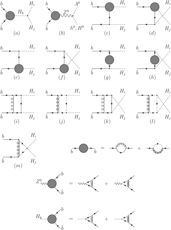
Figure 2: Virtual one-loop Feynman diagrams for $b\bar{b}\rightarrow H_{i}H_{j}$.

The Feynman diagrams for the virtual corrections to $b\bar{b}\rightarrow H_{i}H_{j}$ are shown in Fig. 2. In order to remove the UV divergences, we renormalize the bottom quark mass in the Yukawa couplings and the wave function of the bottom quark, adopting the on-shell renormalization scheme onmass . The relations between the bare bottom quark mass $m_{b0}$, the bare wave function $\psi_{b0}$ and their relevant renormalization constants $\delta m_{b}$, $\delta Z_{bL(R)}$ are defined as

$$m_{b0}=m_{b}+\delta m_{b},$$

$$\psi_{b0}=(1+\delta Z_{bL})^{\frac{1}{2}}\psi_{bL}+(1+\delta Z_{bR})^{\frac{1}{2}}\psi_{bR}.$$ (7)

Calculating the self-energy diagrams in Fig. 2, we obtain the explicit expressions for $\delta m_{b}$ and $\delta Z_{bL(R)}$:

$$\frac{\delta m_{b}}{m_{b}}=-\frac{\alpha_{s}}{4\pi}C_{F}\bigg{\{}3B_{0}(m_{b}^{2},0,m_{b}^{2})-2+\sum_{i=1}^{2}\bigg{[}B_{1}-\frac{m_{\tilde{g}}}{m_{q}}\sin 2\theta_{\tilde{q}}(-1)^{i}B_{0}\bigg{]}(m_{b}^{2},m_{\tilde{g}}^{2},m_{\tilde{b}_{i}}^{2})\bigg{\}},$$

$$\delta Z_{bL}=\frac{\alpha_{s}}{2\pi}C_{F}\sum_{i=1}^{2}(R^{\tilde{b}}_{i1})^{2}B_{1}(0,m_{\tilde{g}}^{2},m_{\tilde{b}_{i}}^{2}),$$

$$\delta Z_{bR}=\frac{\alpha_{s}}{2\pi}C_{F}\sum_{i=1}^{2}(R^{\tilde{b}}_{i2})^{2}B_{1}(0,m_{\tilde{g}}^{2},m_{\tilde{b}_{i}}^{2}),$$

where $C_{F}=4/3$, $B_{0,1}$ are the two-point integrals denner , $m_{\tilde{b}_{1,2}}$ are the sbottom masses, $m_{\tilde{g}}$ is the gluino mass, and $R^{\tilde{b}}$ is a $2\times 2$ matrix defined to rotate the sbottom current eigenstates into the mass eigenstates:

$$\left(\begin{array}[]{c}\tilde{b}_{1}\\ \tilde{b}_{2}\end{array}\right)=R^{\tilde{b}}\left(\begin{array}[]{c}\tilde{b}_{L}\\ \tilde{b}_{R}\end{array}\right),\ \ \ \ \ R^{\tilde{b}}=\left(\begin{array}[]{cc}\cos\theta_{\tilde{b}}&\sin\theta_{\tilde{b}}\\ -\sin\theta_{\tilde{b}}&\cos\theta_{\tilde{b}}\end{array}\right)$$ (8)

with $0\leq\theta_{\tilde{b}}<\pi$ by convention. Correspondingly, the mass eigenvalues $m_{\tilde{b}_{1}}$ and $m_{\tilde{b}_{2}}$ (with $m_{\tilde{b}_{1}}\leq m_{\tilde{b}_{2}}$) are given by

$$\left(\begin{array}[]{cc}m_{\tilde{b}_{1}}^{2}&0\\ 0&m_{\tilde{b}_{2}}^{2}\end{array}\right)=R^{\tilde{b}}M_{\tilde{b}}^{2}(R^{\tilde{b}})^{\dagger},\ \ \ \ \ M_{\tilde{b}}^{2}=\left(\begin{array}[]{cc}m_{\tilde{b}_{L}}^{2}&a_{b}m_{b}\\ a_{b}m_{b}&m_{\tilde{b}_{R}}^{2}\end{array}\right)$$ (13)

with

$$m^{2}_{\tilde{b}_{L}} = M^{2}_{\tilde{Q}}+m_{b}^{2}+m_{Z}^{2}\cos 2\beta C_{bL},$$

$$m^{2}_{\tilde{b}_{R}} = M^{2}_{\tilde{D}}+m_{b}^{2}-m_{Z}^{2}\cos 2\beta C_{bR},$$

$$a_{b} = A_{b}-\mu\tan\beta.$$ (14)

Here $M_{\tilde{b}}^{2}$ is the sbottom mass matrix. $M_{\tilde{Q},\tilde{D}}$ and $A_{b}$ are soft SUSY-breaking parameters and $\mu$ is the higgsino mass parameter.

The renormalized virtual amplitudes can be written as

$$M^{V}_{ij}=M^{unren}_{ij}+M^{con}_{ij}.$$ (15)

Here $M^{unren}_{ij}$ contains the self-energy, vertex and box corrections, and can be written as

$$M^{unren}_{ij}=\sum_{\alpha=a}^{m}\frac{iC_{F}}{16\pi^{2}}g^{2}g_{s}^{2}\bar{v}(p_{b})[f^{\alpha}_{1}P_{L}+f^{\alpha}_{2}P_{R}+\not\!p_{1}(f^{\alpha}_{3}P_{L}+f^{\alpha}_{4}P_{R})]u(p_{a}),$$ (16)

where $\alpha$ denotes the corresponding diagram in Fig. 2, and $f_{l}^{\alpha}$ $(l=1,2,3,4)$ are the form factors given explicitly in Appendix B. $M^{con}_{ij}$ is the corresponding counterterm, and can be separated into $M^{con(s)}_{ij}$, $M^{con(t)}_{ij}$ and $M^{con(u)}_{ij}$, i.e. the counterterms for s, t and u channels, respectively:

$$M^{con}_{ij}=M^{con(s)}_{ij}+M^{con(t)}_{ij}+M^{con(u)}_{ij}$$ (17)

with

$$M^{con(s)}_{ij}=-\frac{ig^{2}Y_{b}m_{Z}}{2c_{W}}[\frac{\delta m_{b}}{m_{b}}+\frac{1}{2}(\delta Z_{bL}+\delta Z_{bR})]\sum_{k=1}^{4}\frac{C_{kij}}{s_{H_{k}}}\bar{v}(p_{b})(a_{k}P_{L}+a_{k}^{\ast}P_{R})u(p_{a})$$

$$\hskip 51.21504pt-\frac{\delta_{i3}g^{2}Z_{j}^{H}}{2c_{W}^{2}(s-m_{Z}^{2})}\bar{v}(p_{b})(\not{\!p}_{1}-\not{\!p}_{2})(C_{bL}\delta Z_{bL}P_{L}+C_{bR}\delta Z_{bR}P_{R})u(p_{a}),$$

$$M^{con(t)}_{ij}=\frac{ig^{2}Y_{b}^{2}}{t}\bar{v}(p_{b})\not{\!p}_{1}[a_{i}a_{j}^{\ast}(2\frac{\delta m_{b}}{m_{b}}+\delta Z_{bL})P_{L}+a_{j}a_{i}^{\ast}(2\frac{\delta m_{b}}{m_{b}}+\delta Z_{bR})P_{R}]u(p_{a}),$$

$$M^{con(u)}_{ij}=\frac{ig^{2}Y_{b}^{2}}{u}\bar{v}(p_{b})\not{\!p}_{2}[a_{j}a_{i}^{\ast}(2\frac{\delta m_{b}}{m_{b}}+\delta Z_{bL})P_{L}+a_{i}a_{j}^{\ast}(2\frac{\delta m_{b}}{m_{b}}+\delta Z_{bR})P_{R}]u(p_{a}).$$ (18)

The ${\cal O}(\alpha_{s})$ virtual corrections to the differential cross section can be expressed as

$$\frac{d^{2}\hat{\sigma}^{V}_{ij}}{dt^{\prime}du^{\prime}}=\frac{1}{1+\delta_{ij}}\frac{\pi S_{\epsilon}}{s^{2}\Gamma(1-\epsilon)}\bigg{(}\frac{t^{\prime}u^{\prime}-sm_{H_{i}}^{2}}{\mu_{r}^{2}s}\bigg{)}^{-\epsilon}\Theta(t^{\prime}u^{\prime}-sm_{H_{i}}^{2})\Theta[s-(m_{H_{i}}+m_{H_{j}})^{2}]$$

$$\hskip 51.21504pt\times\delta(s+t+u-m_{H_{i}}^{2}-m_{H_{j}}^{2})\ 2\ {\rm Re}\overline{(M^{V}_{ij}M^{B\ast}_{ij})},$$ (19)

where the renormalized amplitude $M^{V}_{ij}$ is UV finite, but still contains the infrared (IR) divergences, and is given by

$$M^{V}_{ij}|_{IR}=\frac{\alpha_{s}}{2\pi}\frac{\Gamma(1-\epsilon)}{1-2\epsilon}\bigg{(}\frac{4\pi\mu_{r}^{2}}{s}\bigg{)}^{\epsilon}\bigg{(}\frac{A_{2}^{V}}{\epsilon^{2}}+\frac{A_{1}^{V}}{\epsilon}\bigg{)}M^{B}_{ij},$$ (20)

with

$$A_{2}^{V}=-C_{F},\qquad A_{1}^{V}=-\frac{3}{2}C_{F}.$$ (21)

The coefficients $A_{2}^{V}$ and $A_{1}^{V}$ are constants, and similar to those in the pure Drell-Yan-like processes (without color particles in the final states). These IR divergences include the soft divergences and the collinear divergences. The soft divergences will be cancelled after adding the real corrections, and the remaining collinear divergences can be absorbed into the redefinition of PDFs altarelli , which will be discussed in the following subsections.

When recalculating the above virtual corrections in the DRED scheme, one finds that $\delta Z_{bL}$ and $\delta Z_{bR}$ remain unchanged, however, $\delta m_{b}$ and the form factors have shifts which are, respectively, given by

$$\bigg{(}\frac{\delta m_{b}}{m_{b}}\bigg{)}_{DREG}=\bigg{(}\frac{\delta m_{b}}{m_{b}}\bigg{)}_{DRED}+\frac{\alpha_{s}}{4\pi}C_{F},$$ (22)

and

$$\sum_{\alpha=a}^{m}{f_{1}^{\alpha}}_{DREG}=\sum_{\alpha=a}^{m}{f_{1}^{\alpha}}_{DRED}+\sum_{k=1}^{4}\frac{m_{Z}Y_{b}a_{k}C_{kij}}{c_{W}s_{H_{k}}},$$

$$\sum_{\alpha=a}^{m}{f_{2}^{\alpha}}_{DREG}=\sum_{\alpha=a}^{m}{f_{2}^{\alpha}}_{DRED}+\sum_{k=1}^{4}\frac{m_{Z}Y_{b}a_{k}^{\ast}C_{kij}}{c_{W}s_{H_{k}}},$$

$$\sum_{\alpha=a}^{m}{f_{3}^{\alpha}}_{DREG}=\sum_{\alpha=a}^{m}{f_{3}^{\alpha}}_{DRED}-\frac{\delta_{i3}iZ_{j}^{H}C_{bL}}{c_{W}^{2}(s-m_{Z}^{2})}-\frac{3Y_{b}^{2}}{tu}(ua_{i}a_{j}^{\ast}-ta_{j}a_{i}^{\ast}),$$

$$\sum_{\alpha=a}^{m}{f_{4}^{\alpha}}_{DREG}=\sum_{\alpha=a}^{m}{f_{4}^{\alpha}}_{DRED}-\frac{\delta_{i3}iZ_{j}^{H}C_{bR}}{c_{W}^{2}(s-m_{Z}^{2})}-\frac{3Y_{b}^{2}}{tu}(ua_{j}a_{i}^{\ast}-ta_{i}a_{j}^{\ast}).$$ (23)

Thus it is easy to obtain the following relations:

$${M^{V}_{ij}}_{DREG}={M^{V}_{ij}}_{DRED}-\frac{\alpha_{s}}{4\pi}C_{F}M^{B}_{ij},$$ (24)

$${\sigma^{V}_{ij}}_{DREG}={\sigma^{V}_{ij}}_{DRED}-\frac{\alpha_{s}}{2\pi}C_{F}\sigma^{B}_{ij}+{\cal O}(\alpha^{2}_{s}),$$ (25)

where $M^{B}_{ij}$ and $\sigma^{B}_{ij}$ are independent of the choice of schemes.

III.2 Real gluon emission

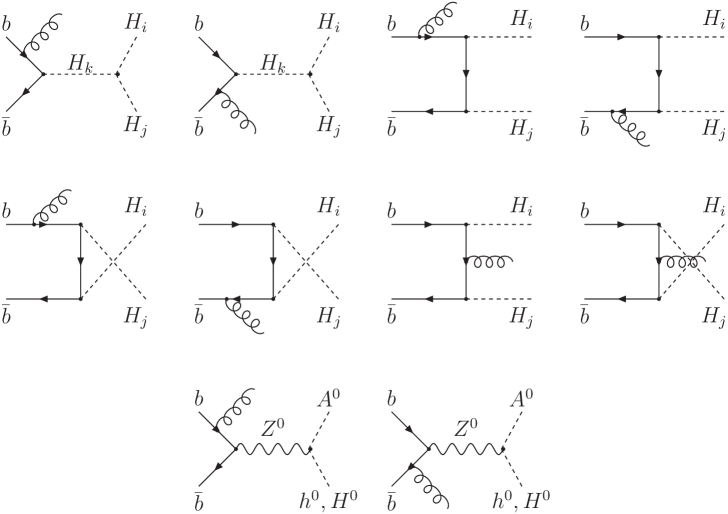
Figure 3: Feynman diagrams for the real gluon emission contributions.

The feynman diagrams for the real gluon emission process $b(p_{a})\bar{b}(p_{b})\rightarrow H_{i}(p_{1})H_{j}(p_{2})+g(p_{3})$ are shown in Fig. 3.

The phase space integration for the real gluon emission will produce soft and collinear singularities, which can be conveniently isolated by slicing the phase space into different regions using suitable cut-offs. In this paper, we use the two cut-off phase space slicing method cutoff , which introduces two arbitrary small cut-offs, i.e. soft cut-off $\delta_{s}$ and collinear one $\delta_{c}$, to decompose the three-body phase space into three regions.

First, the phase space is separated into two regions by the soft cut-off $\delta_{s}$, according to whether the energy of the emitted gluon is soft, i.e. $E_{3}\leq\delta_{s}\sqrt{s}/2$, or hard, i.e. $E_{3}>\delta_{s}\sqrt{s}/2$. Correspondingly, the parton level real cross section $\hat{\sigma}^{R}_{ij}$ can be written as

$$\hat{\sigma}^{R}_{ij}=\hat{\sigma}^{S}_{ij}+\hat{\sigma}^{H}_{ij},$$ (26)

where $\hat{\sigma}^{S}_{ij}$ and $\hat{\sigma}^{H}_{ij}$ are the contributions from the soft and hard regions, respectively. $\hat{\sigma}^{S}$ contains all the soft divergences, which can explicitly be obtained after the integration over the phase space of the emitted gluon. Next, in order to isolate the remaining collinear divergences from $\hat{\sigma}^{H}$, the collinear cut-off $\delta_{c}$ is introduced to further split the hard gluon phase space into two regions, according to whether the Mandelstam variables $u_{1,2}\equiv(p_{a,b}-p_{3})^{2}$ satisfy the collinear condition $-\delta_{c}s<u_{1,2}<0$ or not. We then have

$$\hat{\sigma}^{H}_{ij}=\hat{\sigma}^{HC}_{ij}+\hat{\sigma}^{\overline{HC}}_{ij},$$ (27)

where the hard collinear part $\hat{\sigma}^{HC}_{ij}$ contains the collinear divergences, which also can explicitly be obtained after the integration over the phase space of the emitted gluon. And the hard non-collinear part $\hat{\sigma}^{\overline{HC}}$ is finite and can be numerically computed using standard Monte-Carlo integration techniques Monte , and can be written in the form

$$d\hat{\sigma}^{\overline{HC}}_{ij}=\frac{1}{2s}\overline{|M^{b\bar{b}}_{ij}|}^{2}d\overline{\Gamma}_{3}.$$ (28)

Here $d\overline{\Gamma}_{3}$ is the hard non-collinear region of the three-body phase space, and the explicit expressions for $\overline{|M^{b\bar{b}}_{ij}|}^{2}$ are given in Appendix C.

In the next two subsections, we will discuss in detail the soft and hard collinear gluon emission.

III.2.1 Soft gluon emission

In the limit that the energy of the emitted gluon becomes small, i.e. $E_{3}\leq\delta_{s}\sqrt{s}/2$, the amplitude squared $\overline{|M^{R}_{ij}|}^{2}$ can simply be factorized into the Born amplitude squared times an eikonal factor $\Phi_{eik}$:

$$\overline{|M^{R}_{ij}(b\bar{b}\rightarrow H_{i}H_{j}+g)|}^{2}\stackrel{{\scriptstyle soft}}{{\rightarrow}}(4\pi\alpha_{s}\mu_{r}^{2\epsilon})\overline{|M^{B}_{ij}|}^{2}\Phi_{eik},$$ (29)

where the eikonal factor $\Phi_{eik}$ is given by

$$\Phi_{eik}=C_{F}\frac{s}{(p_{a}\cdot p_{3})(p_{b}\cdot p_{3})}.$$ (30)

Moreover, the phase space in the soft limit can also be factorized:

$$d\Gamma_{3}(b\bar{b}\rightarrow H_{i}H_{j}+g)\stackrel{{\scriptstyle soft}}{{\rightarrow}}d\Gamma_{2}(b\bar{b}\rightarrow H_{i}H_{j})dS,$$ (31)

Here $dS$ is the integration over the phase space of the soft gluon, and is given by cutoff

$$dS=\frac{1}{2(2\pi)^{3-2\epsilon}}\int_{0}^{\delta_{s}\sqrt{s}/2}dE_{3}E_{3}^{1-2\epsilon}d\Omega_{2-2\epsilon}.$$ (32)

The parton level cross section in the soft region can then be expressed as

$$\hat{\sigma}^{S}_{ij}=(4\pi\alpha_{s}\mu_{r}^{2\epsilon})\int d\Gamma_{2}\overline{|M^{B}_{ij}|}^{2}\int dS\Phi_{eik}.$$ (33)

Using the approach of Ref. cutoff , after the integration over the soft gluon phase space, Eq. (33) becomes

$$\hat{\sigma}^{S}_{ij}=\hat{\sigma}^{B}_{ij}\left[\frac{\alpha_{s}}{2\pi}\frac{\Gamma(1-\epsilon)}{\Gamma(1-2\epsilon)}\bigg{(}\frac{4\pi\mu_{r}^{2}}{s}\bigg{)}^{\epsilon}\right]\bigg{(}\frac{A_{2}^{s}}{\epsilon^{2}}+\frac{A_{1}^{s}}{\epsilon}+A_{0}^{s}\bigg{)}$$ (34)

with

$$A_{2}^{s}=2C_{F},\qquad A_{1}^{s}=-4C_{F}\ln\delta_{s},\qquad A_{0}^{s}=4C_{F}\ln^{2}\delta_{s}.$$ (35)

These coefficients are the same as the ones in pure Drell-Yan-like processes, as expected.

III.2.2 Hard collinear gluon emission

In the hard collinear region, $E_{3}>\delta_{s}\sqrt{s}/2$ and $-\delta_{c}s<u_{1,2}<0$, the emitted hard gluon is collinear to one of the incoming partons. As a consequence of the factorization theorems factor1 , the amplitude squared for $b\bar{b}\rightarrow H_{i}H_{j}+g$ can be factorized into the product of the Born amplitude squared and the Altarelli-Parisi splitting function for $b(\bar{b})\rightarrow b(\bar{b})g$ altarelli1 ; factor2 .

$$\overline{|M^{R}_{ij}(b\bar{b}\rightarrow H_{i}H_{j}+g)|}^{2}\stackrel{{\scriptstyle collinear}}{{\rightarrow}}(4\pi\alpha_{s}\mu_{r}^{2\epsilon})\overline{|M^{B}_{ij}|}^{2}\bigg{(}\frac{-2P_{bb}(z,\epsilon)}{zu_{1}}+\frac{-2P_{\bar{b}\bar{b}}(z,\epsilon)}{zu_{2}}\bigg{)},$$ (36)

Here $z$ denotes the fraction of incoming parton $b(\bar{b})$’s momentum carried by parton $b(\bar{b})$ with the emitted gluon taking a fraction $(1-z)$, and $P_{ij}(z,\epsilon)$ are the unregulated splitting functions in $n=4-2\epsilon$ dimensions for $0<z<1$, which can be related to the usual Altarelli-Parisi splitting kernels altarelli1 as follows: $P_{ij}(z,\epsilon)=P_{ij}(z)+\epsilon P_{ij}^{\prime}(z)$, explicitly

$$P_{bb}(z)=P_{\bar{b}\bar{b}}(z)=C_{F}\frac{1+z^{2}}{1-z}+C_{F}\frac{3}{2}\delta(1-z),$$ (37)

$$P_{bb}^{\prime}(z)=P_{\bar{b}\bar{b}}^{\prime}(z)=-C_{F}(1-z)+C_{F}\frac{1}{2}\delta(1-z).$$ (38)

Moreover, the three-body phase space can also be factorized in the collinear limit, and, for example, in the limit $-\delta_{c}s<u_{1}<0$ it has the following form cutoff :

$$d\Gamma_{3}(b\bar{b}\rightarrow H_{i}H_{j}+g)\stackrel{{\scriptstyle collinear}}{{\rightarrow}}d\Gamma_{2}(b\bar{b}\rightarrow H_{i}H_{j};s^{\prime}=zs)\frac{(4\pi)^{\epsilon}}{16\pi^{2}\Gamma(1-\epsilon)}dzdu_{1}[-(1-z)u_{1}]^{-\epsilon}.$$ (39)

Here the two-body phase space is evaluated at a squared parton-parton energy of $zs$. Thus the three-body cross section in the hard collinear region is given by cutoff

$$d\sigma^{HC}_{ij}=d\hat{\sigma}^{B}_{ij}\bigg{[}\frac{\alpha_{s}}{2\pi}\frac{\Gamma(1-\epsilon)}{\Gamma(1-2\epsilon)}(\frac{4\pi\mu_{r}^{2}}{s})^{\epsilon}\bigg{]}(-\frac{1}{\epsilon})\delta_{c}^{-\epsilon}\bigg{[}P_{bb}(z,\epsilon)G_{b/p}(x_{1}/z)G_{\bar{b}/p}(x_{2})$$

$$\hskip 39.83368pt+P_{\bar{b}\bar{b}}(z,\epsilon)G_{\bar{b}/p}(x_{1}/z)G_{b/p}(x_{2})+(x_{1}\leftrightarrow x_{2})\bigg{]}\frac{dz}{z}(\frac{1-z}{z})^{-\epsilon}dx_{1}dx_{2},$$ (40)

where $G_{b(\bar{b})/p}(x)$ is the bare PDF.

III.3 Massless $b(\bar{b})$ emission

In addition to real gluon emission, a second set of real emission corrections to the inclusive cross section for $pp\rightarrow H_{i}H_{j}$ at NLO involves the processes with an additional massless $b(\bar{b})$ in the final state:

$$gb\rightarrow H_{i}H_{j}b,\qquad g\bar{b}\rightarrow H_{i}H_{j}\bar{b}.$$

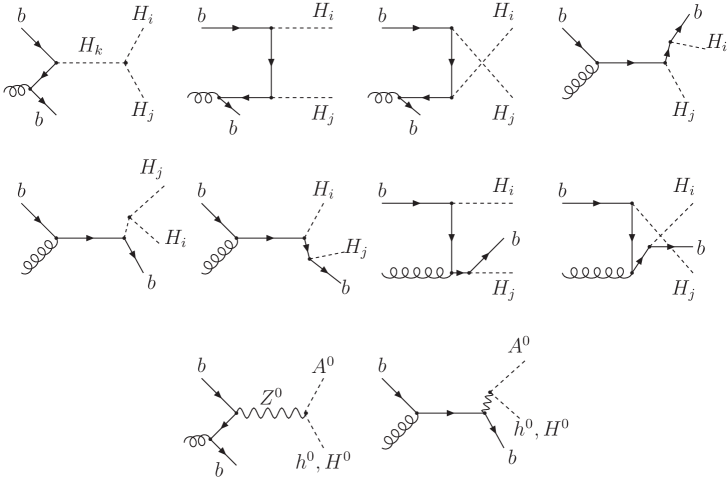
Figure 4: Feynman diagrams for the massless bottom quark emission contributions.

The relevant feynman diagrams for massless $b$ emission are shown in Fig. 4, and the diagrams for $\bar{b}$-emission are similar and omitted here.

Since the contributions from real massless $b(\bar{b})$ emission contain initial state collinear singularities, we also need to use the two cut-off phase space slicing method cutoff to isolate these collinear divergences. But we only split the phase space into two regions, because there are no soft divergences. Consequently, using the approach in Ref. cutoff , the cross sections for the processes with an additional massless $b(\bar{b})$ in the final state can be expressed as

$$d\sigma^{add}_{ij}=\sum_{\alpha=b,\bar{b}}\hat{\sigma}^{\overline{C}}_{ij}(g\alpha\rightarrow H_{i}H_{j}+X)[G_{g/p}(x_{1})G_{\alpha/p}(x_{2})+(x_{1}\leftrightarrow x_{2})]dx_{1}dx_{2}$$

$$\hskip 28.45274pt+d\hat{\sigma}^{B}_{ij}\bigg{[}\frac{\alpha_{s}}{2\pi}\frac{\Gamma(1-\epsilon)}{\Gamma(1-2\epsilon)}(\frac{4\pi\mu^{2}_{r}}{s})^{\epsilon}\bigg{]}(-\frac{1}{\epsilon})\delta_{c}^{-\epsilon}\bigg{[}P_{bg}(z,\epsilon)G_{g/p}(x_{1}/z)G_{\bar{b}/p}(x_{2})$$

$$\hskip 28.45274pt+G_{b/p}(x_{1})P_{\bar{b}g}(z,\epsilon)G_{g/p}(x_{2}/z)+(x_{1}\leftrightarrow x_{2})\bigg{]}\frac{dz}{z}\bigg{(}\frac{1-z}{z}\bigg{)}^{-\epsilon}dx_{1}dx_{2},$$ (41)

where

$$P_{bg}(z)=P_{\bar{b}g}(z)=\frac{1}{2}[z^{2}+(1-z)^{2}],\hskip 56.9055ptP_{bg}^{\prime}(z)=P_{\bar{b}g}^{\prime}(z)=-z(1-z).$$ (42)

The first term in Eq.(III.3) represents the non-collinear cross sections for the two processes, which can also be written in the form ($\alpha=b,\bar{b}$)

$$d\hat{\sigma}^{\overline{C}}_{ij}=\frac{1}{2s}\overline{|M^{g\alpha}_{ij}|}^{2}d\overline{\Gamma}_{3},$$ (43)

where $d\overline{\Gamma}_{3}$ is the three body phase space in the non-collinear region. The explicit expressions for $\overline{|M^{g\alpha}_{ij}|}^{2}$ can be obtained from $\overline{|M^{b\bar{b}}_{ij}|}^{2}$ by crossing symmetry. The second term in Eq.(III.3) represents the collinear singular cross sections.

III.4 Mass factorization

As mentioned above, after adding the renormalized virtual corrections and the real corrections, the parton level cross sections still contain collinear divergences, which can be absorbed into the redefinition of the PDFs at NLO, in general called mass factorization altarelli . This procedure in practice means that first we convolute the partonic cross section with the bare PDF $G_{\alpha/p}(x)$, and then use the renormalized PDF $G_{\alpha/p}(x,\mu_{f})$ to replace $G_{\alpha/p}(x)$. In the $\overline{\rm MS}$ convention, the scale dependent PDF $G_{\alpha/p}(x,\mu_{f})$ is given by cutoff

$$G_{\alpha/p}(x,\mu_{f})=G_{\alpha/p}(x)+\sum_{\beta}(-\frac{1}{\epsilon})\bigg{[}\frac{\alpha_{s}}{2\pi}\frac{\Gamma(1-\epsilon)}{\Gamma(1-2\epsilon)}\bigg{(}\frac{4\pi\mu_{r}^{2}}{\mu_{f}^{2}}\bigg{)}^{\epsilon}\bigg{]}\int_{x}^{1}\frac{dz}{z}P_{\alpha\beta}(z)G_{\beta/p}(x/z).$$ (44)

This replacement will produce a collinear singular counterterm, which is combined with the hard collinear contributions to result in, as the definition in Ref. cutoff , the ${\cal O}(\alpha_{s})$ expression for the remaining collinear contribution:

$$d\sigma^{coll}_{ij}=d\hat{\sigma}^{B}_{ij}\bigg{[}\frac{\alpha_{s}}{2\pi}\frac{\Gamma(1-\epsilon)}{\Gamma(1-2\epsilon)}\bigg{(}\frac{4\pi\mu^{2}_{r}}{s}\bigg{)}^{\epsilon}\bigg{]}\{\tilde{G}_{b/p}(x_{1},\mu_{f})G_{\bar{b}/p}(x_{2},\mu_{f})+G_{b/p}(x_{1},\mu_{f})\tilde{G}_{\bar{b}/p}(x_{2},\mu_{f})$$

$$\hskip 34.14322pt+\sum_{\alpha=b,\bar{b}}\bigg{[}\frac{A_{1}^{sc}(\alpha\rightarrow\alpha g)}{\epsilon}+A_{0}^{sc}(\alpha\rightarrow\alpha g)\bigg{]}G_{b/p}(x_{1},\mu_{f})G_{\bar{b}/p}(x_{2},\mu_{f})$$

$$\hskip 34.14322pt+(x_{1}\leftrightarrow x_{2})\}dx_{1}dx_{2},$$ (45)

where

$$A_{1}^{sc}(b\rightarrow bg)=A_{1}^{sc}(\bar{b}\rightarrow\bar{b}g)=C_{F}(2\ln\delta_{s}+3/2),$$ (46)

$$A_{0}^{sc}=A_{1}^{sc}\ln(\frac{s}{\mu_{f}^{2}}),$$ (47)

$$\tilde{G}_{\alpha/p}(x,\mu_{f})=\sum_{\beta}\int_{x}^{1-\delta_{s}\delta_{\alpha\beta}}\frac{dy}{y}G_{\beta/p}(x/y,\mu_{f})\tilde{P}_{\alpha\beta}(y)$$ (48)

with

$$\tilde{P}_{\alpha\beta}(y)=P_{\alpha\beta}\ln(\delta_{c}\frac{1-y}{y}\frac{s}{\mu_{f}^{2}})-P_{\alpha\beta}^{\prime}(y).$$ (49)

Finally, the NLO total cross section for $pp\rightarrow H_{i}H_{j}$ in the $\overline{MS}$ factorization scheme is

$$\sigma^{NLO}_{ij}=\int\{dx_{1}dx_{2}\bigg{[}G_{b/p}(x_{1},\mu_{f})G_{\bar{b}/p}(x_{2},\mu_{f})+(x_{1}\leftrightarrow x_{2})\bigg{]}(\hat{\sigma}^{B}_{ij}+\hat{\sigma}^{V}_{ij}+\hat{\sigma}^{S}_{ij}+\hat{\sigma}^{\overline{HC}}_{ij})+\sigma^{coll}_{ij}\}$$

$$\hskip 11.38092pt+\sum_{\alpha=b,\bar{b}}\int dx_{1}dx_{2}\bigg{[}G_{g/p}(x_{1},\mu_{f})G_{\alpha/p}(x_{2},\mu_{f})+(x_{1}\leftrightarrow x_{2})\bigg{]}\hat{\sigma}^{\overline{C}}_{ij}(g\alpha\rightarrow H_{i}H_{j}+X).$$ (50)

Note that the above expression contains no singularities since $2A_{2}^{V}+A_{2}^{s}=0$ and $2A_{1}^{V}+A_{1}^{s}+A_{1}^{sc}(b\rightarrow bg)+A_{1}^{sc}(\bar{b}\rightarrow\bar{b}g)=0$.

III.5 Real corrections and NLO total cross sections in the DRED scheme

Above we gave the real corrections and NLO total cross sections in the DREG scheme, and next we show the corresponding results in the DRED scheme, where the contributions from soft gluon emission remain the same, while those from hard collinear gluon emission and massless (anti)quark emission are different. These differences arise from the splitting functions and the PDFs.

First, the splitting functions in the DRED scheme have no $\epsilon$ parts, and we have

$$P_{ij}(z,\epsilon)_{DRED}=P_{ij}(z).$$ (51)

Then from Eq. (45) and (51) we obtain

$${\sigma^{coll}_{ij}}_{DREG}={\sigma^{coll}_{ij}}_{DRED}-\frac{\alpha_{s}}{2\pi}\{\sum_{\beta}\int_{x_{1}}^{1-\delta_{s}\delta_{b\beta}}\frac{dy}{y}G_{\beta/p}(x_{1}/y,\mu_{f}){P^{\prime}}_{b\beta}(y)G_{\bar{b}/p}(x_{2},\mu_{f})$$

$$\hskip 5.69046pt+\sum_{\beta}\int_{x_{2}}^{1-\delta_{s}\delta_{\bar{b}\beta}}\frac{dy}{y}G_{\beta/p}(x_{2}/y,\mu_{f}){P^{\prime}}_{\bar{b}\beta}(y)G_{b/p}(x_{1},\mu_{f})+(x_{1}\leftrightarrow x_{2})\}\hat{\sigma}^{B}dx_{1}dx_{2},$$ (52)

Secondly, the PDFs in the DRED and DREG schemes are related diffPDF :

$$G_{\alpha/p}(x,\mu_{f})_{DREG}=G_{\alpha/p}(x,\mu_{f})_{DRED}+\frac{\alpha_{s}}{2\pi}\sum_{\beta}\int_{x}^{1}\frac{dy}{y}{P^{\prime}}_{\alpha\beta}(x/y).$$ (53)

Substituting into the formula for the Born cross section, we obtain an additional difference at the ${\cal O}(\alpha_{s})$ level arising from the PDFs:

$${\sigma^{B}_{ij}}_{DREG}={\sigma^{B}_{ij}}_{DRED}+\frac{\alpha_{s}}{2\pi}\{\sum_{\beta}\int_{x_{1}}^{1}\frac{dy}{y}G_{\beta/p}(x_{1}/y,\mu_{f})_{DRED}{P^{\prime}}_{b\beta}(y)G_{\bar{b}/p}(x_{2},\mu_{f})_{DRED}$$

$$\hskip 22.76228pt+\sum_{\beta}\int_{x_{2}}^{1}\frac{dy}{y}G_{\beta/p}(x_{2}/y,\mu_{f})_{DRED}{P^{\prime}}_{\bar{b}\beta}(y)G_{b/p}(x_{1},\mu_{f})_{DRED}+(x_{1}\leftrightarrow x_{2})\}\hat{\sigma}^{B}dx_{1}dx_{2}.$$

(54)

Equations (52) and (54) are very similar except for the limits of the integral over y in the two expressions. Substituting the equations (52), (54) and (25) into (50), we obtain the relation of the NLO total cross sections in the two schemes:

$${\sigma^{NLO}_{ij}}_{DREG}={\sigma^{NLO}_{ij}}_{DRED}+\frac{\alpha_{s}}{2\pi}\{\sum_{\beta}\int_{1-\delta_{s}\delta_{b\beta}}^{1}\frac{dy}{y}G_{\beta/p}(x_{1}/y,\mu_{f}){P^{\prime}}_{b\beta}(y)G_{\bar{b}/p}(x_{2},\mu_{f})$$

$$\hskip 34.14322pt+\sum_{\beta}\int_{1-\delta_{s}\delta_{\bar{b}\beta}}^{1}\frac{dy}{y}G_{\beta/p}(x_{2}/y,\mu_{f}){P^{\prime}}_{\bar{b}\beta}(y)G_{b/p}(x_{1},\mu_{f})+(x_{1}\leftrightarrow x_{2})\}\hat{\sigma}^{B}_{ij}dx_{1}dx_{2}$$

$$\hskip 34.14322pt-\frac{\alpha_{s}}{2\pi}C_{F}{\sigma^{B}_{ij}}+{\cal O}(\alpha^{2}_{s}).$$ (55)

Using the explicit expressions for the $\epsilon$ parts of the splitting functions $P^{\prime}$, we find

$${\sigma^{NLO}_{ij}}_{DREG}={\sigma^{NLO}_{ij}}_{DRED}+{\cal O}(\alpha^{2}_{s}).$$ (56)

Therefore, the NLO total cross sections in the two schemes are the same.

III.6 Differential cross section in transverse momentum and invariant mass

In this subsection we present the differential cross section in the transverse momentum $p_{T}$ and the invariant mass. Using the notations defined in Ref. beenakker2 , the differential distribution with respect to $p_{T}$ and $y$ of $H_{i}$ for the processes

$$p(p_{a})+p(p_{b})\rightarrow H_{i}(p_{1})+H_{j}(p_{2})[+g(p_{3})/b(p_{3})/\bar{b}(p_{3})]$$ (57)

is given by

$$\frac{d^{2}\sigma_{ij}}{dp_{T}dy}=2p_{T}S\sum_{\alpha,\beta}\int_{x_{1}^{-}}^{1}dx_{1}\int_{x_{2}^{-}}^{1}dx_{2}x_{1}G_{\alpha/p}(x_{1},\mu_{f})x_{2}G_{\beta/p}(x_{2},\mu_{f})\frac{d^{2}\hat{\sigma}_{ij}}{dt^{\prime}du^{\prime}},$$ (58)

where $\sqrt{S}$ is the total center-of-mass energy of the collider, and

$$p_{T}^{2}=\frac{T_{2}U_{2}}{S}-m_{H_{i}}^{2},\hskip 51.21504pty=\frac{1}{2}\ln(\frac{T_{2}}{U_{2}}),$$

$$x_{1}^{-}=\frac{-T_{2}-m_{H_{i}}^{2}+m_{H_{j}}^{2}}{S+U_{2}},\ \ \ \ \ \ x_{2}^{-}=\frac{-x_{1}U_{2}-m_{H_{i}}^{2}+m_{H_{j}}^{2}}{x_{1}S+T_{2}}$$ (59)

with $T_{2}=(p_{b}-p_{1})^{2}-m_{H_{i}}^{2}$ and $U_{2}=(p_{a}-p_{1})^{2}-m_{H_{i}}^{2}$. The limits of integration over $y$ and $p_{T}$ are

$$-y^{max}(p_{T})\leq y\leq y^{max}(p_{T}),\hskip 42.67912pt0\leq p_{T}\leq p_{T}^{max},$$ (60)

with

$$y^{max}(p_{T})={\rm arccosh}\bigg{(}\frac{S+m_{H_{i}}^{2}-m_{H_{j}}^{2}}{2\sqrt{S(p_{T}^{2}+m_{H_{i}}^{2})}}\bigg{)},$$

$$p_{T}^{max}=\frac{1}{2\sqrt{S}}\sqrt{(S+m_{H_{i}}^{2}-m_{H_{j}}^{2})^{2}-4m_{H_{i}}^{2}S}\ .$$ (61)

The differential distribution with respect to the invariant mass $M_{H_{i}H_{j}}$ is given by

$$\frac{d\sigma}{dM_{H_{i}H_{j}}}=\frac{2M_{H_{i}H_{j}}}{S}\sum_{\alpha,\beta}\frac{d{\cal{L}}_{H_{i}H_{j}}^{\alpha\beta}}{d\tau}\hat{\sigma}_{\alpha\beta}(\tau S),$$ (62)

where $d{\cal{L}}_{H_{i}H_{j}}^{\alpha\beta}/d\tau$ is the parton luminosity:

$$\frac{d{\cal{L}}_{H_{i}H_{j}}^{\alpha\beta}}{d\tau}=\int^{1}_{\tau}\frac{dx}{x}\bigg{[}G_{\alpha/p}(x,\mu_{f})G_{\beta/p}(\tau/x,\mu_{f})\bigg{]},$$ (63)

with

$$M_{H_{i}H_{j}}\equiv\sqrt{(p_{1}+p_{2})^{2}}\geq(m_{H_{i}}+m_{H_{j}}),\qquad\tau\equiv M^{2}_{H_{i}H_{j}}/S.$$ (64)

IV Numerical results and conclusions

In this section, we present the numerical results for total and differential cross sections for pair production of neutral Higgs bosons at the LHC. In our numerical calculations, the SM parameters were taken to be $\alpha_{\rm ew}(m_{W})=1/128$, $m_{W}=80.425$ GeV, $m_{Z}=91.1876$ GeV and $m_{t}=178.1$ GeV parameter . We used the two-loop evaluation for $\alpha_{s}(Q)$ runningalphas $(\alpha_{s}(M_{Z})=0.118)$ and CTEQ6M PDFs CTEQ throughout the calculations of the NLO (LO) cross sections unless specified . Moreover, in order to improve the perturbative calculations, we took the running mass $m_{b}(Q)$ evaluated by the NLO formula runningmb :

$$m_{b}(Q)=U_{6}(Q,m_{t})U_{5}(m_{t},m_{b})m_{b}(m_{b})$$ (65)

with $m_{b}(m_{b})=4.25$ GeV mb . The evolution factor $U_{f}$ is

$$U_{f}(Q_{2},Q_{1})=\bigg{(}\frac{\alpha_{s}(Q_{2})}{\alpha_{s}(Q_{1})}\bigg{)}^{d^{(f)}}\bigg{[}1+\frac{\alpha_{s}(Q_{1})-\alpha_{s}(Q_{2})}{4\pi}J^{(f)}\bigg{]},$$

$$d^{(f)}=\frac{12}{33-2f},\hskip 28.45274ptJ^{(f)}=-\frac{8982-504f+40f^{2}}{3(33-2f)^{2}}.$$ (66)

In addition, to also improve the perturbation calculations, especially for large $\tan\beta$, we made the following SUSY replacements in the tree-level couplings runningmb :

$$m_{b}(Q)\ \ \rightarrow\ \ \frac{m_{b}(Q)}{1+\Delta m_{b}},$$ (67)

$$\Delta m_{b}=\frac{2\alpha_{s}}{3\pi}m_{\tilde{g}}\mu\tan\beta I(m_{\tilde{b}_{1}},m_{\tilde{b}_{2}},m_{\tilde{g}})+\frac{g^{2}m_{t}^{2}}{32\pi^{2}m_{W}^{2}\sin^{2}\beta}\mu A_{t}\tan\beta I(m_{\tilde{t}_{1}},m_{\tilde{t}_{2}},\mu)$$

$$\hskip 28.45274pt-\frac{g^{2}}{16\pi^{2}}\mu M_{2}\tan\beta\sum_{i=1}^{2}\bigg{[}(R^{\tilde{t}}_{i1})^{2}I(m_{\tilde{t}_{i}},M_{2},\mu)+\frac{1}{2}(R^{\tilde{b}}_{i1})^{2}I(m_{\tilde{b}_{i}},M_{2},\mu)\bigg{]}$$ (68)

with

$$I(a,b,c)=\frac{1}{(a^{2}-b^{2})(b^{2}-c^{2})(a^{2}-c^{2})}(a^{2}b^{2}\log\frac{a^{2}}{b^{2}}+b^{2}c^{2}\log\frac{b^{2}}{c^{2}}+c^{2}a^{2}\log\frac{c^{2}}{a^{2}}).$$ (69)

It is necessary, to avoid double counting, to subtract these (SUSY-)QCD corrections from the renormalization constant $\delta m_{b}$ in the following numerical calculations.

For the MSSM parameters, we chose $m_{\frac{1}{2}}$, $m_{0}$, $A_{0}$, $\tan\beta$ and the sign of $\mu$ as input parameters, where $m_{\frac{1}{2}}$, $m_{0}$ and $A_{0}$ are the universal gaugino mass , scalar mass at the GUT scale and the trilinear soft breaking parameter in the superpotential terms, respectively. Specifically, we took $m_{\frac{1}{2}}=170$ GeV, $A_{0}=200$ GeV, and tuned $m_{0}$ to obtain the desired value of $m_{A^{0}}$, while $\tan\beta$ and sign of $\mu$ are free. All other MSSM parameters are determined in the minimal supergravity (mSUGRA) scenario by the program package SUSPECT 2.3 suspect . In particular, we used running $\overline{\rm DR}$ Higgs masses at $m_{Z}$, which include the full one–loop corrections, as well as the two–loop corrections controlled by the strong gauge coupling and the Yukawa couplings of the third generation fermions higgsmass . Moreover, since an $s$-channel resonance can occur in the process $pp\rightarrow h^{0}h^{0}+X$ when $m_{H^{0}}>2m_{h^{0}}$, we adopted the program package HDECAY 3.101 hdecay to determine the total decay widths of the Higgs bosons. For example, in the case of $\tan\beta=40$, $m_{A^{0}}=250$ GeV and $\mu<0$, we have $m_{h^{0}}=108.7$ GeV, $m_{H^{0}}=250.3$ GeV, $\Gamma_{h^{0}}=8$ MeV, $\Gamma_{H^{0}}=13.1$ GeV, $\Gamma_{A^{0}}=13.5$ GeV, $m_{\tilde{g}}=454$ GeV, $m_{\tilde{b}_{1}}=422$ GeV, and $m_{\tilde{b}_{2}}=493$ GeV.

For the renormalization and factorization scales, we always chose $\mu_{r}=m_{\rm av}\equiv(m_{H_{i}}+m_{H_{j}})/2$ and $\mu_{f}=m_{\rm av}$ unless specified.

In Fig. 5, we chose $A^{0}H^{0}$ production through $b\bar{b}$ annihilation as an example to show that it is reasonable to use the two cut-off phase space slicing method in our NLO QCD calculations, i.e. the dependence of the NLO QCD predictions on the arbitrary cut-offs $\delta_{s}$ and $\delta_{c}$ is indeed very weak, as shown in Ref. cutoff . Here $\sigma_{\rm other}$ includes the contributions from the Born cross section and the virtual corrections, which are cut-off independent. Both the soft plus hard collinear contributions and the hard non-collinear contributions depend strongly on the cutoffs and, especially for the small cut-offs ($\delta_{s}<10^{-5}$), each is about ten times larger than the LO total cross section. However, the two contributions ($\sigma_{soft}+\sigma_{hard/coll}+\sigma_{virtual}$ and $\sigma_{hard/non-coll}$) nearly cancel each other completely, especially for the cut-off $\delta_{s}$ between $5\times 10^{-5}$ and $10^{-3}$, where the final results for $\sigma_{NLO}$ are almost independent of the cut-offs and very near 7.7 fb. Therefore, we will take $\delta_{s}=10^{-4}$ and $\delta_{c}=\delta_{s}/50$ in the numerical calculations below.

In Figs. 6–9, we give the total cross sections for $h^{0}h^{0}$, $H^{0}H^{0}$, $A^{0}A^{0}$ and $h^{0}H^{0}$ production, respectively, and compare the $b\bar{b}$-annihilation contributions with the $gg$-fusion contributions hpair0 ; hpair1 ; hpair11 ; hpair2 , which arise from quark and squark loops. In the case of $h^{0}h^{0}$ production, Ref. hpair2 indicated that $b\bar{b}$ annihilation can be more important than $gg$ fusion for large values of $\tan\beta$, but it is not so here (see Fig. 6(a)), which is due to the fact that we have used a much larger decay width for the $H^{0}$ than the one in Ref. hpair2 . However, when $\tan\beta$ is small ($<15$), the contributions of $b\bar{b}$ annihilation still can exceed those of $gg$ fusion (see Fig. 6(b)). As for $H^{0}H^{0}$ (Fig. 7) and $A^{0}A^{0}$ (Fig. 8) production, $b\bar{b}$ annihilation is suppressed by a factor between 2 and 3 in most of the parameter space compared to $gg$ fusion except for $m_{A^{0}}\geq 400$ GeV and $\tan\beta=40$, where the contributions of $b\bar{b}$ annihilation are larger than those of $gg$ fusion, but the corresponding cross sections are very small ($<0.1$ fb). In the case of $H^{0}h^{0}$ production, $b\bar{b}$ annihilation dominates for $m_{A^{0}}>250$ GeV and large values of $\tan\beta$. From Figs. 6–9, we also see that the NLO QCD corrections to the total cross sections for these four processes can enhance the LO results significantly for $\mu>0$, generally by a few tens of percent, while for $\mu<0$, the corrections are relatively small, and are even negative in some parameter regions.

In Figs. 10 and 11, we plot the total cross sections for $pp\rightarrow A^{0}h^{0},\ A^{0}H^{0}$ at the LHC as functions of $m_{A^{0}}$ and $\tan\beta$, and compare the $b\bar{b}$ annihilation contributions with $gg$ fusion hpair0 ; hpair1 ; hpair11 ; hpair2 and $q\bar{q}$ annihilation hpair0 . In the case of $A^{0}h^{0}$ production, the $b\bar{b}$-annihilation contributions dominate for large values of $\tan\beta$. For example, when $\tan\beta=40$ and $m_{A^{0}}>250$ GeV (see Fig. 10(a)), the contributions are several times larger than $gg$ fusion contributions, and at least two orders of magnitude larger than $q\bar{q}$ annihilation contributions. However, for small values of $\tan\beta$, $gg$ fusion dominates, as shown in Fig. 10(b). In the case of $A^{0}H^{0}$ production, after including the NLO QCD corrections, the cross section for $b\bar{b}$ annihilation is lager than those of the other two mechanisms for large values of $\tan\beta$ and most values of $m_{A^{0}}$. Moreover, the $b\bar{b}$-annihilation contributions can exceed 100 fb for $\tan\beta=40$ and $m_{A^{0}}<150$ GeV, as shown in Fig. 11(a). From Figs. 10 and 11, we also see that the NLO QCD corrections to the total cross section for these two processes can enhance the LO results significantly for $\mu>0$, generally by a few tens of percent, while for $\mu<0$, the corrections are negative and relatively small.

Fig. 12 gives the dependence of the ratio $K$ (defined as the ratio of the NLO total cross sections to the LO ones) on $m_{A^{0}}$ for $A^{0}h^{0}/A^{0}H^{0}$ production through $b\bar{b}$ annihilation based on the results shown in Fig. 10(a) and 11(a). We see that in general the ratio $K$ is negative, and becomes larger with the increasing $m_{A^{0}}$. For example, when $m_{A^{0}}$ varies from 120 GeV to 500 GeV, the ratio $K$ increases from 0.7 to 0.95 for $A^{0}h^{0}$ production (Fig. 12(a)), and from 0.75 to 0.88 for $A^{0}H^{0}$ production (Fig. 12(b)). The contributions to the ratio $K$ come from three IR finite parts: the LO total cross sections, the pure QCD corrections and the SUSY-QCD virtual corrections, the latter two of which are also shown in the figure.

The main parts of $b\bar{b}$ annihilation contributions for large values of $\tan\beta$ originate from the Yukawa coupling $b-b-\phi$, so the results are sensitive to the bottom quark mass. In Fig. 13, we show the effects of the choices of $m_{b}$ on the total cross section for $A^{0}H^{0}$ production through $b\bar{b}$ annihilation, assuming $\tan\beta=40$, $m_{1/2}=170$ GeV, $A_{0}=200$ GeV and $\mu<0$. We considered three different bottom quark masses, (i) $\overline{\rm MS}$ bottom quark mass at the scale of the $\overline{\rm MS}$ mass, i.e. $m_{b}(m_{b})=4.25$ GeV, (ii) QCD running bottom quark mass $m_{b}(\mu_{r})$, and (iii) QCD running plus SUSY improved bottom quark running mass. They can have very different values. For example, in this figure, when $m_{A^{0}}=250$ GeV, they are 4.25 GeV, 2.69 GeV and 3.17 GeV, which leads to the LO total cross sections being 12.5 fb, 5 fb and 9.8 fb, respectively. Moreover, from Fig. 13, we see that the NLO QCD corrections can be very large in the cases of $m_{b}(m_{b})$ and QCD running $m_{b}$. For this reason we use the SUSY improved bottom quark running mass, which improves the convergence of the perturbation calculations, especially for large values of $\tan\beta$, as shown in Fig. 13.

Fig. 14 gives the dependence of the total cross section for $A^{0}H^{0}$ production through $b\bar{b}$ annihilation at the LHC on the renormalization/factorization scale for $\mu_{r}=\mu_{f}$. In the case of $\mu>0$, the scale dependence of both the LO and the NLO total cross sections is relatively weak. And for $\mu<0$, the scale dependence of the total cross sections is reduced when going from LO to NLO. For example, the cross sections vary by $\pm 20\%$ at LO but by $\pm 13\%$ at NLO in the region $0.5<\mu_{f}/m_{\rm av}<2.0$.

Since another source of uncertainty arises from the different choice of PDFs, in Fig. 15 we show the total cross sections for $A^{0}H^{0}$ production through $b\bar{b}$ annihilation as functions of $m_{A^{0}}$ for three different PDFs. We first use the 41 CTEQ6.1 PDF sets 61cteq to estimate the uncertainty in the LO total cross sections. The LO results using the CTEQ6M PDFs lie between the maximum and the minimum. The NLO total cross sections are then calculated using three different PDF sets, one of which is CTEQ6M, and the other two are the ones that gave the maximum and minimum LO uncertainties. Observe that in this case the uncertainty arising from the choice of PDFs increases with the increasing $m_{A^{0}}$. Moreover, the dependence of the total cross sections on PDFs is not decreased from LO to NLO.

In Fig. 16, we display differential cross sections as the functions of the transverse momentum $p_{T}$ of the $A^{0}$ and the invariant mass $M_{A^{0}H^{0}}$, which are given by Eqs.(58) and (62), respectively, for the $A^{0}H^{0}$ production through $b\bar{b}$ annihilation. In the case of $\mu<0$, we find that the NLO QCD corrections reduce the LO differential cross sections except for low $p_{T}$, while in the case of $\mu>0$, the corrections always enhance the LO results.

In conclusion, we have calculated the complete NLO inclusive total cross sections for pair production of neutral Higgs bosons through $b\bar{b}$ annihilation in the MSSM at the LHC. In our calculations, we used both the DREG scheme and the DRED scheme and found that the NLO total cross sections in the above two schemes are the same. Our results show that the $b\bar{b}$ annihilation contributions can exceed those of $gg$ fusion and $q\bar{q}$ annihilation for $h^{0}H^{0}$, $A^{0}h^{0}$ and $A^{0}H^{0}$ production when $\tan\beta$ is large. For $\mu>0$ the NLO corrections enhance the LO total cross sections significantly, and can reach a few tens percent, while for $\mu<0$ the corrections are relatively small and negative in most of parameter space. Moreover, the NLO QCD corrections reduce the dependence of these total cross sections on the renormalization/factorization scale, especially for $\mu<0$. We also used the CTEQ6.1 PDF sets to estimate the uncertainty in both the LO and NLO total cross sections, and found that the uncertainty arising from the choice of PDFs increases with the increasing $m_{A^{0}}$.

Appendix A

In this appendix, we give the relevant Feynman couplings higgshunter .

1. $H_{i}-b-\bar{b}:$ $igY_{b}(a_{i}P_{L}+a_{i}^{\ast}P_{R})$

$$a_{1}=-\frac{1}{\sqrt{2}}\cos\alpha,\ \ \ \ \ a_{2}=\frac{1}{\sqrt{2}}\sin\alpha,\ \ \ \ \ a_{3}=-\frac{i}{\sqrt{2}}\sin\beta,\ \ \ \ \ a_{4}=\frac{i}{\sqrt{2}}\cos\beta,$$

where $\alpha$ is the mixing angle in the CP-even neutral Higgs boson sector.

2. $H_{j}-Z-A^{0}:$ $gZ^{H}_{j}(p_{A^{0}}-p_{H_{j}})^{\mu}/(2c_{W})$

$$Z^{H}_{1}=-\sin(\beta-\alpha),\ \ \ \ \ Z^{H}_{2}=\cos(\beta-\alpha),\ \ \ \ \ Z^{H}_{3}=Z^{H}_{4}=0.$$

Here we define the outgoing four–momenta of $A^{0}$ and $H_{j}$ positive.

3. $H_{k}-H_{i}-H_{j}:$ $igm_{Z}C_{kij}/(2c_{W})$

$$C_{111}=-3\cos 2\alpha\cos(\alpha+\beta),\qquad C_{112}=2\sin 2\alpha\cos(\alpha+\beta)+\sin(\alpha+\beta)\cos 2\alpha,$$

$$C_{122}=-2\sin 2\alpha\sin(\alpha+\beta)+\cos(\alpha+\beta)\cos 2\alpha,\qquad C_{133}=\cos 2\beta\cos(\alpha+\beta),$$

$$C_{134}=\sin 2\beta\cos(\alpha+\beta),\qquad C_{144}=-\cos 2\beta\cos(\alpha+\beta),$$

$$C_{222}=-3\cos 2\alpha\sin(\alpha+\beta),\qquad C_{233}=-\cos 2\beta\sin(\alpha+\beta),$$

$$C_{244}=\cos 2\beta\sin(\alpha+\beta),\qquad C_{234}=-\sin 2\beta\sin(\alpha+\beta).$$

The indexes $i,j$ and $k$ of $C_{kij}$ are symmetric, and other coefficients are zero.

4. $H_{k}-\tilde{b}_{l}-\tilde{b}_{m}$: $igG^{k}_{lm}\equiv ig[R^{\tilde{b}}\hat{G}^{k}(R^{\tilde{b}})^{T}]_{lm}$

$$\hat{G}^{1}=\left(\begin{array}[]{cc}-\frac{m_{Z}}{c_{W}}\cos(\alpha+\beta)C_{bL}-\sqrt{2}m_{b}Y_{b}\cos\alpha&-\frac{1}{\sqrt{2}}Y_{b}(A_{b}\cos\alpha-\mu\sin\alpha)\\ -\frac{1}{\sqrt{2}}Y_{b}(A_{b}\cos\alpha-\mu\sin\alpha)&\frac{m_{Z}}{c_{W}}\cos(\alpha+\beta)C_{bR}-\sqrt{2}m_{b}Y_{b}\cos\alpha\end{array}\right),$$

$$\hat{G}^{2}=\left(\begin{array}[]{cc}\frac{m_{Z}}{c_{W}}\sin(\alpha+\beta)C_{bL}+\sqrt{2}m_{b}Y_{b}\sin\alpha&\frac{1}{\sqrt{2}}Y_{b}(A_{b}\sin\alpha+\mu\cos\alpha)\\ \frac{1}{\sqrt{2}}Y_{b}(A_{b}\sin\alpha+\mu\cos\alpha)&-\frac{m_{Z}}{c_{W}}\sin(\alpha+\beta)C_{bR}+\sqrt{2}m_{b}Y_{b}\sin\alpha\end{array}\right),$$

$$\hat{G}^{3}=i\frac{m_{b}}{2m_{W}}\left(\begin{array}[]{cc}0&-A_{b}\tan\beta-\mu\\ A_{b}\tan\beta+\mu&0\end{array}\right),$$

$$\hat{G}^{4}=i\frac{m_{b}}{2m_{W}}\left(\begin{array}[]{cc}0&A_{b}-\mu\tan\beta\\ -A_{b}+\mu\tan\beta&0\end{array}\right).$$

5. $Z^{0}-\tilde{b}_{l}-\tilde{b}_{m}$: $-igZ^{\tilde{b}}_{ml}(p_{\tilde{b}_{m}}+p_{\tilde{b}_{l}})^{\mu}/c_{W}$

$$Z^{\tilde{b}}_{ml}=R^{\tilde{b}}_{m1}R^{\tilde{b}}_{l1}C_{bL}+R^{\tilde{b}}_{m2}R^{\tilde{b}}_{l2}C_{bR},$$

where $p_{\tilde{b}_{m}}$ and $p_{\tilde{b}_{l}}$ are the four–momenta of $\tilde{b}_{m}$ and $\tilde{b}_{m}$ in direction of the charge flow.

6. $H_{i}-H_{j}-\tilde{b}_{l}-\tilde{b}_{m}$: $ig^{2}G^{ij}_{lm}\equiv ig^{2}[R^{\tilde{b}}\hat{G}^{ij}(R^{\tilde{b}})^{T}]_{lm}$

$$\hat{G}^{11}_{lm}=-\frac{1}{2}\left(\frac{\cos 2\alpha}{c_{W}^{2}}C_{bL}+\frac{m_{b}^{2}\cos^{2}\alpha}{m_{W}^{2}\cos^{2}\beta}\right)\delta_{l1}\delta_{m1}+\frac{1}{2}\left(\frac{\cos 2\alpha}{c_{W}^{2}}C_{bR}-\frac{m_{b}^{2}\cos^{2}\alpha}{m_{W}^{2}\cos^{2}\beta}\right)\delta_{l2}\delta_{m2},$$

$$\hat{G}^{22}_{lm}=\frac{1}{2}\left(\frac{\cos 2\alpha}{c_{W}^{2}}C_{bL}-\frac{m_{b}^{2}\sin^{2}\alpha}{m_{W}^{2}\cos^{2}\beta}\right)\delta_{l1}\delta_{m1}-\frac{1}{2}\left(\frac{\cos 2\alpha}{c_{W}^{2}}C_{bR}+\frac{m_{b}^{2}\sin^{2}\alpha}{m_{W}^{2}\cos^{2}\beta}\right)\delta_{l2}\delta_{m2},$$

$$\hat{G}^{33}_{lm}=\frac{1}{2}\left(\frac{\cos 2\beta}{c_{W}^{2}}C_{bL}-\frac{m_{b}^{2}\tan^{2}\beta}{m_{W}^{2}}\right)\delta_{l1}\delta_{m1}-\frac{1}{2}\left(\frac{\cos 2\beta}{c_{W}^{2}}C_{bR}+\frac{m_{b}^{2}\tan^{2}\beta}{m_{W}^{2}}\right)\delta_{l2}\delta_{m2},$$

$$\hat{G}^{44}_{lm}=-\frac{1}{2}\left(\frac{\cos 2\beta}{c_{W}^{2}}C_{bL}+\frac{m_{b}^{2}}{m_{W}^{2}}\right)\delta_{l1}\delta_{m1}+\frac{1}{2}\left(\frac{\cos 2\beta}{c_{W}^{2}}C_{bR}-\frac{m_{b}^{2}}{m_{W}^{2}}\right)\delta_{l2}\delta_{m2},$$

$$\hat{G}^{12}_{lm}=\frac{\sin 2\alpha}{2}\left[\left(\frac{C_{bL}}{c_{W}^{2}}+\frac{m_{b}^{2}}{2m_{W}^{2}\cos^{2}\beta}\right)\delta_{l1}\delta_{m1}-\left(\frac{C_{bR}}{c_{W}^{2}}-\frac{m_{b}^{2}}{2m_{W}^{2}\cos^{2}\beta}\right)\delta_{l2}\delta_{m2}\right],$$

$$\hat{G}^{34}_{lm}=\frac{\sin 2\beta}{2}\left[\left(\frac{C_{bL}}{c_{W}^{2}}+\frac{m_{b}^{2}}{2m_{W}^{2}\cos^{2}\beta}\right)\delta_{l1}\delta_{m1}-\left(\frac{C_{bR}}{c_{W}^{2}}-\frac{m_{b}^{2}}{2m_{W}^{2}\cos^{2}\beta}\right)\delta_{l2}\delta_{m2}\right].$$

The indexes $i$ and $j$ of $G^{ij}_{lm}$ are symmetric, and other coefficients are zero.

Appendix B

In this appendix, we collect the explicit expressions for the nonzero form factors in Eq.(16). For simplicity, we introduce the following abbreviations for the Passarino-Veltman integrals, which are defined as in Ref. denner except that we take internal masses squared as arguments:

$$B_{0}^{a(\alpha)}=B_{0}(\alpha,0,0),$$

$$B_{0}^{b(\alpha)}=B_{0}(\alpha,m_{\tilde{g}}^{2},m_{\tilde{b}_{l}}^{2}),$$

$$C_{p(q)}^{a}=C_{p(q)}(0,0,s,0,0,0),$$

$$C_{p(q)}^{b(\alpha)}=C_{p(q)}(0,\alpha,0,m_{\tilde{g}}^{2},m_{\tilde{b}_{l}}^{2},m_{\tilde{b}_{m}}^{2}),$$

$$C_{p(q)}^{c(\alpha r)}=C_{p(q)}(0,m_{H_{r}}^{2},\alpha,0,0,0),$$

$$C_{p(q)}^{d(\alpha r)}=C_{p(q)}(0,m_{H_{r}}^{2},\alpha,m_{\tilde{g}}^{2},m_{\tilde{b}_{m}}^{2},m_{\tilde{b}_{l}}^{2}),$$

$$C_{p(q)}^{e(\alpha)}=C_{p(q)}(\alpha,m_{H_{i}}^{2},m_{H_{j}}^{2},0,0,0),$$

$$D_{p(q)}^{a(\alpha)}=D_{p(q)}(\alpha,m_{H_{j}}^{2},s,0,0,m_{H_{i}}^{2},0,0,0,0),$$

$$D_{p(q)}^{b(\alpha)}=D_{p(q)}(0,s,m_{H_{i}}^{2},\alpha,0,m_{H_{j}}^{2},m_{\tilde{g}}^{2},m_{\tilde{b}_{l}}^{2},m_{\tilde{b}_{m}}^{2},m_{\tilde{b}_{n}}^{2}).$$

Many functions above contain soft and collinear singularities, but all the Passarino-Veltman integrals can be reduced to the scalar functions $B_{0}$, $C_{0}$ and $D_{0}$. Here we present the explicit expressions for $C_{0}$ and $D_{0}$, which contain the singularities, and were used in our calculations:

$$C_{0}^{a}=\frac{C_{\epsilon}}{s}\bigg{[}\frac{1}{\epsilon^{2}}-\frac{2\pi^{2}}{3}\bigg{]},$$

$$C^{c(\alpha r)}_{0}=\frac{C_{\epsilon}}{\alpha-m_{H_{r}}^{2}}\bigg{[}\frac{1}{\epsilon}\ln\bigg{(}\frac{-\alpha}{m_{H_{r}}^{2}}\bigg{)}+\frac{1}{2}\ln^{2}\bigg{(}\frac{s}{m_{H_{r}}^{2}}\bigg{)}-\frac{1}{2}\ln^{2}\bigg{(}\frac{s}{-\alpha}\bigg{)}-\frac{\pi^{2}}{2}\bigg{]},$$

$$D^{a(\alpha)}_{0}=\frac{C_{\epsilon}}{s\alpha}\bigg{[}\frac{1}{\epsilon^{2}}+\frac{2}{\epsilon}\ln\bigg{(}\frac{m_{H_{i}}m_{H_{j}}}{-\alpha}\bigg{)}+\frac{2\pi^{2}}{3}\bigg{]}-\frac{2C_{\epsilon}}{s\alpha}\Bigg{\{}{\rm Li}_{2}\bigg{(}\frac{s+\alpha-m^{2}_{H_{i}}}{s}\bigg{)}-{\rm Li}_{2}\bigg{(}\frac{s-m_{H_{i}}^{2}}{s}\bigg{)}$$

$$\hskip 31.2982pt-{\rm Li}_{2}\bigg{[}\frac{-s\alpha}{(s-m_{H_{i}}^{2})(m_{H_{i}}^{2}-\alpha)}\bigg{]}+{\rm Li}_{2}\bigg{(}\frac{-\alpha}{s-m_{H_{i}}^{2}}\bigg{)}+{\rm Li}_{2}\bigg{(}\frac{m^{2}_{H_{j}}}{m^{2}_{H_{j}}-\alpha}\bigg{)}$$

$$\hskip 31.2982pt-\frac{1}{2}\ln^{2}\bigg{[}\frac{-s\alpha}{(s-m_{H_{i}}^{2})(m_{H_{i}}^{2}-\alpha)}\bigg{]}+\frac{1}{2}\ln^{2}\bigg{(}\frac{-\alpha}{s-m_{H_{i}}^{2}}\bigg{)}+\ln\bigg{(}\frac{m_{H_{i}}^{2}-\alpha}{s}\bigg{)}\ln\bigg{(}\frac{s+\alpha-m^{2}_{H_{i}}}{-\alpha}\bigg{)}$$

$$\hskip 31.2982pt-\frac{1}{2}\ln\bigg{(}\frac{m_{H_{i}}^{2}-\alpha}{s}\bigg{)}\ln\bigg{(}\frac{sm^{2}_{H_{j}}}{\alpha^{2}}\bigg{)}-\frac{1}{4}\ln^{2}\bigg{(}\frac{sm^{2}_{H_{j}}}{\alpha^{2}}\bigg{)}+\frac{1}{4}\ln^{2}\bigg{(}\frac{m^{2}_{H_{i}}}{s}\bigg{)}$$

$$\hskip 31.2982pt+\frac{1}{2}\ln\bigg{(}\frac{m^{2}_{H_{j}}}{s}\bigg{)}\ln\bigg{(}\frac{m_{H_{i}}^{2}-\alpha}{m^{2}_{H_{i}}}\bigg{)}+\frac{1}{2}\ln^{2}\bigg{(}\frac{m^{2}_{H_{j}}}{m^{2}_{H_{j}}-\alpha}\bigg{)}\Bigg{\}},$$

where we define $C_{\epsilon}=(4\pi\mu^{2}_{r}/s)^{\epsilon}\Gamma(1-\epsilon)/\Gamma(1-2\epsilon)$, and note the explicit expression for $D^{a(\alpha)}_{0}$ is in agreement with the one in Ref. d0 .

There are the following relations between the form factors:

$$f^{\alpha}_{2,4}=f^{\alpha}_{1,3}(a_{i,j,k}\leftrightarrow a_{i,j,k}^{\ast},C_{bL}\leftrightarrow C_{bR},R_{l1}^{\tilde{b}}\leftrightarrow R_{l2}^{\tilde{b}},R_{m1}^{\tilde{b}}\leftrightarrow R_{m2}^{\tilde{b}}).$$

Thus we will only present the explicit expressions of $f_{1}^{\alpha}$ and $f_{3}^{\alpha}$. Corresponding to diagrams (a)–(m) in Fig. 2, the form factors are

$$f^{a}_{1}=\sum_{k=1}^{4}\frac{m_{Z}C_{kij}}{c_{W}s_{H_{k}}}\{Y_{b}a_{k}[s(C_{0}^{a}+2C_{1}^{a}+(2-\epsilon)C_{12}^{a})+4(\epsilon-2)C_{00}^{a}+1]$$

$$\hskip 28.45274pt-\sum_{l,m=1}^{2}m_{\tilde{g}}G_{lm}^{k}R_{m1}^{\tilde{b}}R_{l2}^{\tilde{b}}C_{0}^{b(s)}\},$$

$$f^{b}_{1}=\sum_{l,m=1}^{2}\frac{im_{\tilde{g}}Z_{j}^{H}Z_{lm}^{\tilde{b}}R_{m1}^{\tilde{b}}R_{l2}^{\tilde{b}}}{c_{W}^{2}(s-m_{Z}^{2})}[(u-t)(C_{0}^{b(s)}+C_{1}^{b(s)}+C_{2}^{b(s)})+(m_{H_{j}}^{2}-m_{H_{i}}^{2})(C_{1}^{b(s)}-C_{2}^{b(s)})],$$

$$f^{b}_{3}=\frac{-iZ_{j}^{H}}{c_{W}^{2}(s-m_{Z}^{2})}\{C_{bL}[s(2C_{0}^{a}+4C_{1}^{a}+2(1-\epsilon)C_{12}^{a})-4(1-\epsilon)C_{00}^{a}-1]$$

$$\hskip 28.45274pt+\sum_{l,m=1}^{2}4R_{l1}^{\tilde{b}}R_{m1}^{\tilde{b}}Z_{lm}^{\tilde{b}}C_{00}^{b(s)}\},$$

$$f^{c}_{1}+f^{e}_{1}=-\sum_{l,m=1}^{2}2Y_{b}(a_{j}G_{lm}^{i}R^{\tilde{b}}_{l1}R^{\tilde{b}}_{m1}C_{2}^{d(ti)}+a_{i}G_{ml}^{j}R^{\tilde{b}}_{l2}R^{\tilde{b}}_{m2}C_{2}^{d(tj)}),$$

$$f^{c}_{3}+f^{e}_{3}=\frac{2Y_{b}}{t}\{Y_{b}a_{i}a_{j}^{\ast}\sum_{r=i,j}[t(C_{0}^{c(tr)}+C_{1}^{c(tr)}+2C_{12}^{c(tr)}+2C_{22}^{c(tr)}+3C_{2}^{c(tr)})-t\epsilon(C_{12}^{c(tr)}$$

$$\hskip 42.67912pt+C_{22}^{c(tr)}+C_{2}^{c(tr)})+4(2-\epsilon)C_{00}^{c(tr)}-m_{H_{r}}^{2}(C_{0}^{c(tr)}+C_{1}^{c(tr)}+(2-\epsilon)C_{12}^{c(tr)}+C_{2}^{c(tr)})$$

$$\hskip 42.67912pt-1]+\sum_{l,m=1}^{2}m_{\tilde{g}}(a_{j}^{\ast}G^{i}_{lm}R^{\tilde{b}}_{l2}R^{\tilde{b}}_{m1}C_{0}^{d(ti)}+a_{i}G^{j}_{ml}R^{\tilde{b}}_{m1}R^{\tilde{b}}_{l2}C_{0}^{d(tj)})\},$$

$$f_{1}^{d}+f_{1}^{f}=-\sum_{l,m=1}^{2}2Y_{b}(a_{j}G^{i}_{ml}R^{\tilde{b}}_{l2}R^{\tilde{b}}_{m2}C_{2}^{d(ui)}+a_{i}G^{j}_{lm}R^{\tilde{b}}_{l1}R^{\tilde{b}}_{m1}C_{2}^{d(uj)}),$$

$$f_{3}^{d}+f_{3}^{f}=-\frac{2Y_{b}}{u}\{Y_{b}a_{j}a_{i}^{\ast}\sum_{r=i,j}[u(C_{0}^{c(ur)}+C_{1}^{c(ur)}+2C_{12}^{c(ur)}+2C_{22}^{c(ur)}+3C_{2}^{c(ur)})-u\epsilon(C_{12}^{c(ur)}$$

$$\hskip 42.67912pt+C_{22}^{c(ur)}+C_{2}^{c(ur)})+4(2-\epsilon)C_{00}^{c(ur)}-m_{H_{r}}^{2}(C_{0}^{c(ur)}+C_{1}^{c(ur)}+(2-\epsilon)C_{12}^{c(ur)}+C_{2}^{c(ur)})$$

$$\hskip 42.67912pt-1]+\sum_{l,m=1}^{2}m_{\tilde{g}}[a_{i}^{\ast}G^{j}_{lm}R^{\tilde{b}}_{l2}R^{\tilde{b}}_{m1}C_{0}^{d(uj)}+a_{j}G^{i}_{ml}R^{\tilde{b}}_{l1}R^{\tilde{b}}_{m2}C_{0}^{d(ui)}]\},$$

$$f_{1}^{g}+f_{1}^{h}=-\sum_{l=1}^{2}2Y_{b}^{2}a_{i}a_{j}R^{\tilde{b}}_{l1}R^{\tilde{b}}_{l2}\frac{m_{\tilde{g}}}{tu}(tB_{0}^{b(u)}+uB_{0}^{b(t)}),$$

$$f_{3}^{g}+f_{3}^{h}=Y_{b}^{2}\{\frac{1-\epsilon}{tu}(ta_{j}a_{i}^{\ast}B_{0}^{a(u)}-ua_{i}a_{j}^{\ast}B_{0}^{a(t)})+\sum_{l=1}^{2}(R^{\tilde{b}}_{l2})^{2}[\frac{a_{i}a_{j}^{\ast}}{t^{2}}((m_{\tilde{g}}^{2}-m_{\tilde{b}_{l}}^{2})(B_{0}^{b(0)}$$

$$\hskip 42.67912pt-B_{0}^{b(t)})-tB_{0}^{b(t)})+\frac{a_{j}a_{i}^{\ast}}{u^{2}}((m_{\tilde{g}}^{2}-m_{\tilde{b}_{l}}^{2})(B_{0}^{b(u)}-B_{0}^{b(0)})+uB_{0}^{b(u)})]\},$$

$$f^{i}_{3}=2Y_{b}^{2}a_{i}a_{j}^{\ast}[C_{0}^{c(ti)}+C_{0}^{c(tj)}-(1+\epsilon)C_{0}^{e(s)}-sD_{0}^{a(t)}+(u-t\epsilon)D_{1}^{a(t)}],$$

$$f^{j}_{1}=-\sum_{l,m,n=1}^{2}2m_{\tilde{g}}G^{i}_{nm}G^{j}_{ln}R^{\tilde{b}}_{l2}R^{\tilde{b}}_{m1}D_{0}^{b(t)},$$

$$f^{j}_{3}=\sum_{l,m,n=1}^{2}2G^{i}_{nm}G^{j}_{ln}R^{\tilde{b}}_{l1}R^{\tilde{b}}_{m1}D_{3}^{b(t)},$$

$$f^{k}_{3}=-2Y_{b}^{2}a_{j}a_{i}^{\ast}[C_{0}^{c(ui)}+C_{0}^{c(uj)}-(1+\epsilon)C_{0}^{e(s)}-sD_{0}^{a(u)}+(t-u\epsilon)D_{1}^{a(u)}],$$

$$f^{l}_{1}=-\sum_{l,m,n=1}^{2}2m_{\tilde{g}}G^{i}_{mn}G^{j}_{nl}R^{\tilde{b}}_{m2}R^{\tilde{b}}_{l1}D_{0}^{b(u)},$$

$$f^{l}_{3}=-\sum_{l,m,n=1}^{2}2G^{i}_{mn}G^{j}_{nl}R^{\tilde{b}}_{l1}R^{\tilde{b}}_{m1}D_{3}^{b(u)},$$

$$f^{m}_{1}=\sum_{l,m=1}^{2}2m_{\tilde{g}}G^{ij}_{lm}R^{\tilde{b}}_{l2}R^{\tilde{b}}_{m1}C_{0}^{b(s)}.$$

Appendix C

In this Appendix, we collect the explicit expressions for the amplitudes squared for the radiation of a real gluon.The results for massless $b(\bar{b})$ emission can be obtained by crossing symmetry. Since these expressions are only used for the hard non-collinear parts of the real corrections in Eq.(28) and Eq.(43), they have no singularities and can be calculated in $n=4$ dimensions.

For simplicity, we define the following invariants:

$$s_{3}=(p_{2}+p_{3})^{2},\qquad s_{4}=(p_{1}+p_{3})^{2},\qquad s_{5}=(p_{1}+p_{2})^{2},$$

$$t=(p_{b}-p_{2})^{2},\qquad t^{\prime}=(p_{b}-p_{3})^{2},\qquad u=(p_{a}-p_{2})^{2},$$

$$u^{\prime}=(p_{a}-p_{3})^{2},\qquad u_{6}=(p_{b}-p_{1})^{2},\qquad u_{7}=(p_{a}-p_{1})^{2},$$

. Then for real gluon emission we find

$$\overline{|M^{b\bar{b}}_{ij}|}^{2}=g^{4}g_{s}^{2}\left(\overline{|M^{(HH)}_{ij}|}^{2}+\overline{|M^{(ZZ)}_{ij}|}^{2}+\overline{|M^{(Zt)}_{ij}|}^{2}+\overline{|M^{(Zu)}_{ij}|}^{2}+\overline{|M^{(tt)}_{ij}|}^{2}+\overline{|M^{(tu)}_{ij}|}^{2}+\overline{|M^{(uu)}_{ij}|}^{2}\right),$$

with

$$\overline{|M^{(HH)}_{ij}|}^{2}=\frac{2m_{Z}^{2}Y_{b}^{2}}{c_{W}^{2}}\sum_{k,l=1}^{4}(a_{k}a_{l}^{\ast}+a_{k}^{\ast}a_{l})C_{kij}C_{lij}\frac{(s+t^{\prime}-u^{\prime})(s-t^{\prime}+u^{\prime})}{t^{\prime}u^{\prime}s_{H_{k}}s_{H_{l}}^{\ast}},$$

$$\overline{|M^{(ZZ)}_{ij}|}^{2}=\frac{\delta_{i3}(Z_{j}^{H})^{2}(C_{bL}^{2}+C_{bR}^{2})}{2c_{W}^{4}(s_{5}-m_{Z}^{2})^{2}t^{\prime}u^{\prime}}\{s_{4}u_{6}(s+t^{\prime})+s_{4}u_{7}(s+u^{\prime})+u_{6}u_{7}(2s+t^{\prime}+u^{\prime})-t^{\prime}u_{7}^{2}$$

$$\hskip 28.45274pt-u_{6}^{2}u^{\prime}-m_{H_{i}}^{2}[t^{\prime}(s_{4}+t^{\prime}+2u_{6}-u_{7})+u^{\prime}(u^{\prime}+s_{4}-u_{6}+2u_{7})+s(2s+2s_{4}+2t^{\prime}$$

$$\hskip 28.45274pt+3u_{6}+3u_{7}+2u^{\prime})+m_{H_{i}}^{2}(4s+t^{\prime}+u^{\prime})]\},$$

$$\overline{|M^{(Zt)}_{ij}|}^{2}=\frac{i\delta_{i3}Y_{b}^{2}Z_{j}^{H}}{c_{W}^{2}(s_{5}-m_{Z}^{2})}(C_{bR}a_{j}a_{i}^{\ast}+C_{bL}a_{i}a_{j}^{\ast})\{\frac{2}{tt^{\prime}u_{7}}(s+t^{\prime}+u_{6}-m_{H_{i}}^{2})[m_{H_{i}}^{2}(2s+2s_{4}+t^{\prime}$$

$$\hskip 28.45274pt+2(u_{6}+2u_{7}+u^{\prime})-4m_{H_{i}}^{2})-(2s_{4}+t^{\prime}+2u_{6})u_{7}]$$

$$\hskip 28.45274pt-\frac{1}{t^{\prime}u_{7}}[ss_{4}+u_{7}(4s_{4}+t^{\prime})-u_{6}u^{\prime}-m_{H_{i}}^{2}(s+4s_{4}+t^{\prime}+4u_{7}+3u^{\prime}-4m_{H_{i}}^{2})]$$

$$\hskip 28.45274pt-\frac{2}{tu_{7}u^{\prime}}(u_{7}-m_{H_{i}}^{2})[(2s_{4}+2u_{7}+3u^{\prime}-4m_{H_{i}}^{2})(m_{H_{i}}^{2}-u_{6})-(s+t^{\prime})(u^{\prime}-2m_{H_{i}}^{2})]$$

$$\hskip 28.45274pt+\frac{1}{t^{\prime}u_{7}u^{\prime}}[2u_{6}-2u_{7}-u^{\prime})(u_{6}u^{\prime}-t^{\prime}u_{7}+(t^{\prime}-u^{\prime})m_{H_{i}}^{2})+s(3u^{\prime}+m_{H_{i}}^{2}(4s+4t^{\prime}$$

$$\hskip 28.45274pt+6(u_{6}+u_{7})-4u_{6}u_{7}-8m_{H_{i}}^{2})+s_{4}(u^{\prime}-2u_{6}-2u_{7}+4m_{H_{i}}^{2}))]$$

$$\hskip 28.45274pt-\frac{1}{tu^{\prime}}[s_{3}(s+4t)-t^{\prime}u+tu^{\prime}-m_{H_{j}}^{2}(s+4s_{3}+4t+3t^{\prime}+u^{\prime}-4m_{H_{j}}^{2})]$$

$$\hskip 28.45274pt+\frac{1}{tt^{\prime}u^{\prime}}[s(s_{3}(t^{\prime}-2t-2u)-4tu)+(2t+t^{\prime}-2u)(tu^{\prime}-t^{\prime}u)+m_{H_{j}}^{2}((2t+t^{\prime}$$

$$\hskip 28.45274pt-2u)(t^{\prime}-u^{\prime})+s(4s+4s_{3}+6t+3t^{\prime}+6u+4u^{\prime}-8m_{H_{j}}^{2}))]\},$$

$$\overline{|M^{(tt)}_{ij}|}^{2}=16Y_{b}^{4}|a_{i}|^{2}|a_{j}|^{2}\{\frac{2}{tt^{\prime}u_{7}^{2}}(s+t^{\prime}+u_{6}-m_{H_{i}}^{2})[u_{7}(s_{4}+u_{6})-m_{H_{i}}^{2}(s+s_{4}+u_{6}+2u_{7}$$

$$\hskip 28.45274pt+u^{\prime}-2m_{H_{i}}^{2})]-\frac{1}{tt^{\prime}u_{7}u^{\prime}}[(u_{6}-u_{7}-u^{\prime})(u_{6}u^{\prime}-t^{\prime}u_{7}+m_{H_{i}}^{2}(t^{\prime}-u^{\prime}))$$

$$\hskip 28.45274pt-s(2u_{6}u_{7}+s_{4}(u_{6}+u_{7}-u^{\prime}))+sm_{H_{i}}^{2}(2s+2s_{4}+2t^{\prime}+3u_{6}+3u_{7}+u^{\prime}-4m_{H_{i}}^{2})]$$

$$\hskip 28.45274pt+\frac{2}{t^{2}u_{7}u^{\prime}}(u_{7}-m_{H_{i}}^{2})[(s+t^{\prime}+2u_{6}-2m_{H_{i}}^{2})(m_{H_{i}}^{2}-u^{\prime})+(m_{H_{i}}^{2}-u_{6})(s_{4}+u_{7})]$$

$$\hskip 28.45274pt+\frac{1}{t^{2}u_{7}^{2}}[u_{7}((s+t^{\prime})(s_{4}+u_{7})-u_{6}u^{\prime})-m_{H_{i}}^{2}(t^{\prime}(s_{4}+u^{\prime}-m_{H_{i}}^{2})+u_{7}(s+2t^{\prime}-u^{\prime}))]$$

$$\hskip 28.45274pt+\frac{1}{t^{2}u^{\prime}}[s_{3}t-m_{H_{j}}^{2}(s_{3}+t+t^{\prime}-m_{H_{j}}^{2})]+\frac{1}{t^{\prime}u_{7}^{2}}[s_{4}u_{7}-m_{H_{i}}^{2}(s_{4}+u_{7}+u^{\prime}-m_{H_{i}}^{2})]\},$$

$$\overline{|M^{(tu)}_{ij}|}^{2}=16Y_{b}^{4}a_{i}^{2}a_{j}^{\ast 2}\{\frac{1}{tu_{6}u^{\prime}}[t^{\prime}u_{7}-u_{6}u^{\prime}-(s_{4}-m_{H_{i}}^{2})(s+2u_{6})+m_{H_{i}}^{2}(2s_{4}+t^{\prime}+u^{\prime}-2m_{H_{i}}^{2})]$$

$$\hskip 28.45274pt+\frac{2}{tuu_{6}u_{7}}m_{H_{i}}^{2}m_{H_{j}}^{2}+\frac{2}{tu_{6}u^{\prime}uu_{7}}(tu_{6}-m_{H_{i}}^{2}m_{H_{j}}^{2})[u(u_{7}-m_{H_{i}}^{2})+u_{7}(u-m_{H_{i}}^{2})]$$

$$\hskip 28.45274pt-\frac{1}{t^{\prime}uu_{7}}[(s_{4}-m_{H_{i}}^{2})(s+2u_{7})+t^{\prime}u_{7}-u_{6}u^{\prime}-m_{H_{i}}^{2}(2s_{4}+t^{\prime}+u^{\prime}-2m_{H_{i}}^{2})]$$

$$\hskip 28.45274pt-\frac{2}{t^{\prime}uu_{6}u_{7}}(u_{6}-m_{H_{i}}^{2})[(m_{H_{i}}^{2}-u_{7})(s_{4}+t^{\prime}+u_{6})+m_{H_{i}}^{2}(s+2u_{7}+u^{\prime}-2m_{H_{i}}^{2})]$$

$$\hskip 28.45274pt+\frac{1}{t^{\prime}u_{6}u_{7}u^{\prime}}[(u_{6}-u_{7})(u_{6}u^{\prime}-t^{\prime}u_{7})-s(2u_{6}u_{7}+s_{4}(u_{6}+u_{7}))+m_{H_{i}}^{2}((u_{6}-u_{7})(t^{\prime}-u^{\prime})$$

$$\hskip 28.45274pt+s(2s+2s_{4}+2t^{\prime}+3u_{6}+3u_{7}+2u^{\prime}-4m_{H_{i}}^{2}))]+\frac{2}{tt^{\prime}uu_{7}}(t-m_{H_{j}}^{2})(uu_{7}-m_{H_{i}}^{2}m_{H_{j}}^{2})$$

$$\hskip 28.45274pt+\frac{1}{tt^{\prime}uu^{\prime}}[(t-u)(tu^{\prime}-t^{\prime}u)-s(2tu+s_{3}(t+u))+m_{H_{j}}^{2}((t-u)(t^{\prime}-u^{\prime})+s(2s$$

$$\hskip 28.45274pt+2s_{3}+3t+2t^{\prime}+3u+2u^{\prime}-4m_{H_{j}}^{2}))]\}.$$

Figure 5: Dependence of the total cross sections for $A^{0}H^{0}$ production through $b\bar{b}$ annihilation at the LHC on the cut-off $\delta_{s}$, assuming $m_{A^{0}}=250$ GeV, $\tan\beta=40$, $m_{1/2}=170$ GeV, $A_{0}=200$ GeV, $\mu<0$ and $\delta_{c}=\delta_{s}/50$.

Figure 6: Total cross sections for the $h^{0}h^{0}$ production at the LHC (a) as functions of $m_{A^{0}}$ for $\tan\beta=40$, $\mu<0$ (starting from $m_{A^{0}}=120$ GeV) and $\tan\beta=40$, $\mu>0$ (starting from $m_{A^{0}}=210$ GeV), and (b) as functions of $\tan\beta$ for $m_{A^{0}}=250$ GeV, assuming $m_{1/2}=170$ GeV and $A_{0}=200$ GeV.

Figure 7: Total cross sections for the $H^{0}H^{0}$ production at the LHC (a) as functions of $m_{A^{0}}$ for $\tan\beta=40$, $\mu<0$ (starting from $m_{A^{0}}=120$ GeV) and $\tan\beta=40$, $\mu>0$ (starting from $m_{A^{0}}=210$ GeV), and (b) as functions of $\tan\beta$ for $m_{A^{0}}=250$ GeV, assuming $m_{1/2}=170$ GeV and $A_{0}=200$ GeV.

Figure 8: Total cross sections for the $A^{0}A^{0}$ production at the LHC (a) as functions of $m_{A^{0}}$ for $\tan\beta=40$, $\mu<0$ (starting from $m_{A^{0}}=120$ GeV) and $\tan\beta=40$, $\mu>0$ (starting from $m_{A^{0}}=210$ GeV), and (b) as functions of $\tan\beta$ for $m_{A^{0}}=250$ GeV, assuming $m_{1/2}=170$ GeV and $A_{0}=200$ GeV.

Figure 9: Total cross sections for the $H^{0}h^{0}$ production at the LHC (a) as functions of $m_{A^{0}}$ for $\tan\beta=40$, $\mu<0$ (starting from $m_{A^{0}}=120$ GeV) and $\tan\beta=40$, $\mu>0$ (starting from $m_{A^{0}}=210$ GeV), and (b) as functions of $\tan\beta$ for $m_{A^{0}}=250$ GeV, assuming $m_{1/2}=170$ GeV and $A_{0}=200$ GeV.

Figure 10: Total cross sections for the $A^{0}h^{0}$ production at the LHC (a) as functions of $m_{A^{0}}$ for $\tan\beta=40$, $\mu<0$ (starting from $m_{A^{0}}=120$ GeV) and $\tan\beta=40$, $\mu>0$ (starting from $m_{A^{0}}=210$ GeV), and (b) as functions of $\tan\beta$ for $m_{A^{0}}=250$ GeV, assuming $m_{1/2}=170$ GeV and $A_{0}=200$ GeV.

Figure 11: Total cross sections for the $A^{0}H^{0}$ production at the LHC (a) as functions of $m_{A^{0}}$ for $\tan\beta=40$, $\mu<0$ (starting from $m_{A^{0}}=120$ GeV) and $\tan\beta=40$, $\mu>0$ (starting from $m_{A^{0}}=210$ GeV), and (b) as functions of $\tan\beta$ for $m_{A^{0}}=250$ GeV, assuming $m_{1/2}=170$ GeV and $A_{0}=200$ GeV.

Figure 12: $K=\sigma_{NLO}/\sigma_{LO}$ for the $A^{0}h^{0}/A^{0}H^{0}$ production through $b\bar{b}$ annihilation at the LHC as a function of $m_{A^{0}}$, assuming $\tan\beta=40$, $m_{1/2}=170$ GeV, $A_{0}=200$ GeV and $\mu<0$.

Figure 13: Dependence of the total cross sections for the $A^{0}H^{0}$ production through $b\bar{b}$ annihilation at the LHC on $m_{A^{0}}$ and $m_{b}$, assuming $\tan\beta=40$, $m_{1/2}=170$ GeV, $A_{0}=200$ GeV and $\mu<0$.

Figure 14: Dependence of the total cross sections for the $A^{0}H^{0}$ production through $b\bar{b}$ annihilation at the LHC on renormalization/factorization scale, assuming $\tan\beta=40$, $m_{1/2}=170$ GeV, $A_{0}=200$ GeV and $\mu<0$.

Figure 15: The PDF dependence of the total cross sections for the $A^{0}H^{0}$ production through $b\bar{b}$ annihilation at the LHC, assuming $\tan\beta=40$, $m_{1/2}=170$ GeV, $A_{0}=200$ GeV and $\mu<0$.

Figure 16: Differential cross sections in the transverse momentum $p_{T}$ of $A^{0}$ and the invariant mass $M_{A^{0}H^{0}}$ for the $A^{0}H^{0}$ production through $b\bar{b}$ annihilation at the LHC, assuming $m_{A^{0}}=250$ GeV, $\tan\beta=40$, $m_{1/2}=170$ GeV and $A_{0}=200$ GeV.

References

- (1) H. P. Nilles, Phys. Rep. 110 (1984) 1; H. E. Haber and G. L. Kane, Phys. Rep. 117 (1985) 75; A. B. Lahanas and D. V. Nanopoulos, Phys. Rep. 145 (1987) 1; Supersymmetry, Vols. 1 and 2, ed. S. Ferrara (North Holland/World Scientific, Singapore, 1987); For a recent review, consult S. Dawson, TASI-97 lectures, hep-ph/9712464.
- (2) F. Gianotti, M. L. Mangano, and T. Virdee, hep-ph/0204087.
- (3) T. Hambye and K. Riesselmann, Phys. Rev. D 55 (1997) 7255 .
- (4) Particle Data Group, S. Eidelman et al., Phys. Lett. B 592 (2004) 1.
- (5) H. E. Haber and R. Hempfling, Phys. Rev. Lett. 66 (1991) 1815; Y. Okada, M. Yamaguchi and T. Yanagida, Prog. Theor. Phys. 85 (1991) 1; J. Ellis, G. Ridolfi and F. Zwirner, Phys. Lett. B257 (1991) 83; S. Heinemeyer, hep-ph/0407244.
- (6) D. Denegri et al., hep-ph/0112045; A. Djouadi, Pramana 62 (2004) 191.
- (7) H. M. Georgi, S. L. Glashow, M. E. Machacek and D. V. Nanopoulos, Phys. Rev. Lett. 40 (1978) 692; M. Spira, A. Djouadi, D. Graudenz and P. M. Zerwas, Phys. Lett. B 318 (1993) 347; Nucl. Phys. B 453 (1995) 17; S. Dawson, A. Djouadi and M. Spira, Phys. Rev. Lett. 77 (1996) 16; A. Djouadi and M. Spira, Phys. Rev. D 62 (2000) 014004; R. V. Harlander and W. B. Kilgore, Phys. Rev. Lett. 88 (2002) 201801; JHEP 0210 (2002) 017; C. Anastasiou and K. Melnikov, Nucl. Phys. B 646 (2002) 220; Phys. Rev. D 67 (2003) 037501; V. Ravindran, J. Smith and W. L. van Neerven, Nucl. Phys. B 665 (2003) 325; S. Catani, D. de Florian, M. Grazzini and P. Nason, JHEP 0307 (2003) 028; R. V. Harlander and M. Steinhauser, Phys. Lett. B 574 (2003) 258; Phys. Rev. D 68 (2003) 111701; JHEP 0409 (2004) 066; A. Kulesza, G. Sterman and W. Vogelsang, Phys. Rev. D 69 (2004) 014012.
- (8) R. N. Cahn and S. Dawson, Phys. Lett. B 136 (1984) 196; G. Altarelli, B. Mele and F. Pitolli, Nucl. Phys. B 287 (1987) 205; T. Han, G. Valencia and S. Willenbrock, Phys. Rev. Lett. 69 (1992) 3274.
- (9) S. L. Glashow, D. V. Nanopoulos and A. Yildiz, Phys. Rev. D 18 (1978) 1724; R. Kleiss, Z. Kunszt and W. J. Stirling, Phys. Lett. B 253 (1991) 269; T. Han and S. Willenbrock, Phys. Lett. B 273 (1991) 167.
- (10) S. Dawson, S. Dittmaier and M. Spira, Phys. Rev. D 58 (1998) 115012.
- (11) T. Plehn, M. Spira and P. M. Zerwas, Nucl. Phys. B 479 (1996) 46; Nucl. Phys. B 531 (1998) 655(E).
- (12) A. Belyaev, M. Drees, O. J. P. Éboli, J. K. Mizukoshi and S. F. Novaes, Phys. Rev. D 60 (1999) 075008.
- (13) A. A. Barrientos Bendezú and B. A. Kniehl, Phys. Rev. D 64 (2001) 035006.
- (14) Z. Kunszt, Nucl. Phys. B 247 (1984) 339; W. Beenakker et al., Phys. Rev. Lett. 87 (2001) 201805; Nucl. Phys. B 653 (2003) 151; L. Reina and S. Dawson, Phys. Rev. Lett. 87 (2001) 201804; S. Dawson, L. H. Orr, L. Reina and D. Wackeroth, Phys. Rev. D 67 (2003) 071503.
- (15) J. Campbell, et al., hep-ph/0405302.
- (16) D. Dicus, T. Stelzer, Z. Sullivan and S. Willenbrock, Phys. Rev. D 59 (1999) 094016; C. Balazs, H.-J. He and C.-P. Yuan, Phys. Rev. D 60 (1999) 114001; F. Maltoni, Z. Sullivan and S. Willenbrock, Phys. Rev. D 67 (2003) 093005; R. V. Harlander and W B. Kilgore, Phys. Rev. D 68 (2003) 013001.
- (17) J. Campbell, R. K. Ellis, F. Maltoni and S. Willenbrock, Phys. Rev. D 67 (2003) 095002; S. Dawson, C. B. Jackson, L. Reina and D. Wackeroth, Phys. Rev. Lett. 94 (2005) 031802.
- (18) R. Raitio and W. W. Wada, Phys. Rev. D 19 (1979) 941; C. Balázs, et al., Phys. Rev. D 59 (1999) 055016; E. Boos and T. Plehn, Phys. Rev. D 69 (2004) 094005; S. Dawson, C. B. Jackson, L. Reina and D. Wackeroth, Phys. Rev. D 69 (2004) 074027; S. Dittmaier, M. Krämer and M. Spira, Phys. Rev. D 70 (2004) 074010.
- (19) M. A. G. Aivazis, J. C. Collins, F. I. Olness and W. K. Tung, Phys. Rev. D 50 (1994) 3102; J. C. Collins, Phys. Rev. D 58 (1998) 094002; M. Krämer, F. I. Olness and D. E. Soper, Phys. Rev. D 62 (2000) 096007.
- (20) G. ’t Hooft and M. Veltman, Nucl. Phys. B 44 (1972) 189.
- (21) M. Chanowitz, M. Furman and I. Hinchliffe, Nucl. Phys. B 159 (1979) 225.
- (22) Z. Bern, A. De Freitas, L. Dixon and H. L. Wong, Phys. Rev. D 66 (2002) 085002.
- (23) A. Sirlin, Phys. Rev. D 22 (1980) 971; W. J. Marciano and A. Sirlin, Phys. Rev. D 22 (1980) 2695; Phys. Rev. D 31 (1985) 213 (E); A. Sirlin and W. J. Marciano, Nucl. Phys. B 189 (1981) 442; K. I. Aoki et al., Prog. Theor. Phys. Suppl. 73 (1982) 1.
- (24) A. Denner, Fortschr. Phys. 41 (1993) 4.
- (25) G. Altarelli, R. K. Ellis, G. Martinelli, Nucl. Phys. B 157 (1979) 461; J. C. Collins, D. E. Soper and G. Sterman, in: Perturbative Quantum Chromodynamics, ed. A.H. Mueller (World Scientific, 1989).
- (26) B. W. Harris and J. F. Owens, Phys. Rev. D 65 (2002) 094032.
- (27) G. P. Lepage, J. Comp. Phys. 27 (1978) 192.
- (28) J. C. Collins, D. E. Soper and G. Sterman, Nucl. Phys. B 261 (1985) 104; G. T. Bodwin, Phys. Rev. D 31 (1985) 2616; Phys. Rev. D 34 (1986) 3932 (E).
- (29) G. Altarelli and G. Parisi, Nucl. Phys. B 126 (1977) 298.
- (30) R. K. Ellis, D. A. Ross and A. E. Terrano, Nucl. Phys. B 178 (1981) 421; L. J. Bergmann, in: Next-to-leading-log QCD calculation of symmetric dihadron production (Ph.D. thesis, Florida State University, 1989); Z. Kunszt and D. E. Soper, Phys. Rev. D 46 (1992) 192; M. L. Mangano, P. Nason and G. Ridolfi, Nucl. Phys. B 373 (1992) 295.
- (31) B. kamal, Phys. Rev. D 53 (1996) 1142.
- (32) W. Beenakker, R. Höpker, M. Spira and P. M. Zerwas, Nucl. Phys. B 492 (1997) 51.
- (33) S. G. Gorishny, A. L. Kataev, S. A. Larin and L. R. Surguladze, Mod. Phys. Lett. A 5 (1990) 2703; Phys. Rev. D 43 (1991) 1633; A. Djouadi, M. Spira and P. M. Zerwas, Z. Phys. C 70 (1996) 427; A. Djouadi, J. Kalinowski, M. Spira, Comput. Phys. Commun. 108 (1998) 56; M. Spira, Fortschr. Phys. 46 (1998) 203.
- (34) J. Pumplin, D. R. Stump, J. Huston, H. L. Lai, P. Nadolsky and W. K. Tung, JHEP 0207 (2002) 012.
- (35) M. Carena, D. Garcia, U. Nierste, C. E. M. Wagner, Nucl. Phys. B 577 (2000) 88.
- (36) M. Beneke and A. Signer, Phys. Lett. B 471 (1999) 233; A. H. Hoang, Phys. Rev. D 61 (2000) 034005.
- (37) A. Djouadi, J. L Kneur and G. Moultaka, hep-ph/0211331.
- (38) B. C. Allanach, A. Djouadi, J. L. Kneur, W. Porod and P. Slavich, JHEP 0409 (2004) 044.
- (39) A. Djouadi, J. Kalinowski and M. Spira, Comp. Phys. Commun. 108 (1998) 56.
- (40) D. Stump et al., JHEP 0310 (2003) 046.
- (41) J. F. Gunion, H. E. Haber, G. Kane and S. Dawson, The Higgs Hunter’s Guide (ADDison–Wesley, Redwood City, CA, 1990).
- (42) J. Ohnemus, Phys. Rev. D 44 (1991) 3477.