Improvement of the hot QCD pressure by the minimal sensitivity criterion

Abstract

The principles of minimal sensitivity (PMS) criterion is applied to the perturbative free energy density, or pressure, of hot QCD, which include the $\sim g_{s}^{6}\ln g_{s}$ and part of the $\sim g_{s}^{6}$ terms. Applications are made separately to the short- and long-distance parts of the pressure. Comparison with the lattice results, at low temperatures, shows that the resultant “optimal” approximants are substantially improved when compared to the $\overline{\mbox{MS}}$ results. In particular, for the realistic case of three quark flavors, the “optimal” approximants are comparable with the lattice results.

1 Introduction

In statistical physics, the free energy density, or pressure, plays a central role. At high temperature, the perturbative expansion of the pressure of the quark-gluon plasma is known to fifth order [1] in $g_{s}$ (the QCD coupling constant) and partially to sixth order [2]. These results are reliable only when $g_{s}$ is sufficiently small. Because of the asymptotic freedom of QCD, this is achieved at high temperature $T\gtrsim 2$ GeV which is order of magnitude larger than the critical temperature ($T_{c}$) of the QCD phase transition. For $T_{c}\lesssim T\lesssim 2$ GeV, the accuracy of the approximation, within the $\overline{\mbox{MS}}$ scheme, does not improve by the inclusion of higher order terms (convergence issue). Moreover, the unphysical dependence on the renormalization scale $\mu$ is strong. With the traditional choice $\mu=2\pi T$, the truncated perturbation series for the pressure, in the $\overline{\mbox{MS}}$ scheme, does not reconcile with the lattice results ($0.3$ GeV $\lesssim T\lesssim 0.5$ GeV). To get rid of these dilemmas, various kinds of resummations are proposed. Among those are quasi-particle models [3], $\Phi$-derivative approximations [4], screened perturbation theory [5, 6], hard thermal loop perturbation theory [7], optimizations based on the principles of minimal sensitivity (PMS) and the fastest apparent convergence (FAC) criterions [6], and the Padé type resummation and its variants [8, 9].

In this paper, putting aside the convergence issue, we will obtain the “optimal” approximants for the pressure $p$ through an application of the PMS criterion [10]. Throughout this paper, for the expression $p$ (in massless QCD), we use the one given in Ref. 9):

$$p=p_{E}+p_{M}+p_{G}\,,$$

where $p_{E}$, $p_{M}$, and $p_{G}$ come, in respective order, from the hard ($\sim T$), soft ($\sim g_{s}T$), and supersoft ($\sim g_{s}^{2}T$) energy regions. The scales $g_{s}T$ and $g^{2}_{s}T$ are the color-electric and color-magnetic screening scales, respectively. A crucial observation made in Ref. 9) is that the “short-distance pressure” $p_{E}$ and the “long-distance pressure” $p_{M+G}$ ($\equiv p_{M}+p_{G}$) are separately physical quantities, and thus both, when calculated to all orders of perturbation theory, are independent of the renormalization scheme. Then we will apply the PMS criterion to $p_{E}$ and $p_{M+G}$ separately.

In §2, a brief review of the PMS criterion is given. Then, we present the perturbation expansion of $p_{E}$ and $p_{M+G}$ in the form given in Ref. 9), which is taken as the basis of our analysis. In §3, we apply the PMS criterion to $p_{E}$ and $p_{M+G}$ separately and find the optimal approximants. In §4, we compare our results with the lattice results and the $\overline{\mbox{MS}}$ results. §5 is devoted to discussion and conclusion.

2 Preliminaries

2.1 Brief review of the Principles of Minimal Sensitivity (PMS) (Ref. 10))

The couplant $\alpha_{s}=g_{s}^{2}/(4\pi)$ in massless QCD runs according to the renormalization group equation,

$$\mu\frac{\partial\alpha_{s}}{\partial\mu}=\beta(\alpha_{s})=-\alpha_{s}^{2}\sum_{j=0}^{\infty}\beta_{j}\alpha_{s}^{j}\,.$$ (1)

Here $\mu$ is the renormalization scale and

$$\beta_{0}=\frac{1}{2\pi}\left(11-\frac{2}{3}\,n_{f}\right)\,,$$

$$\beta_{1}=\frac{1}{4\pi^{2}}\left(51-\frac{19}{3}\,n_{f}\right)\,,$$ (2)

with $n_{f}$ is number of quark flavors. The renormalization schemes can be labelled by a countable infinity of parameters ($\mu$, $\beta_{2}$, $\beta_{3}$, …). [$\beta_{0}$ and $\beta_{1}$ are independent of the renormalization scheme.] In the $\overline{\mbox{MS}}$ scheme,

$$(\beta_{2})_{\overline{\mbox{\scriptsize{MS}}}}=\frac{1}{64\pi^{3}}\left(2857-\frac{5033}{9}\,n_{f}+\frac{325}{27}\,n_{f}^{2}\right)\,.$$ (3)

The dependence of $\alpha_{s}$ on $\beta_{j}$ ($j=2,3,...$) is governed by

$$\frac{\partial\alpha_{s}}{\partial\beta_{j}} = -\beta(\alpha_{s})\int_{0}^{\alpha_{s}}\frac{x^{j+2}}{\left(\beta(x)\right)^{2}}\,dx\;\;\left(\equiv\gamma_{j}(\alpha_{s})\right)\,,$$ (4)

$$= \frac{2\pi}{9(j-1)}\alpha_{s}^{j+1}+...\;\;\;\;\;\;\;\;\;\;(j=2,3,...)\,.$$ (5)

It is to be noted that a change in $\mu$ results in a change in $\alpha_{s}$ of $O(\alpha_{s}^{2})$ while a change in $\beta_{i}$ $(i=2,3,...)$ results in a change in $\alpha_{s}$ of $O(\alpha_{s}^{i+1})$. The running $\alpha_{s}=\alpha_{s}(\mu,\beta_{2},\beta_{3},...)$ is obtained by solving Eqs. (1) and (4) under the boundary condition that is provided by the experiment.

Let ${\cal R}$ be some physical quantity, ${\cal R}=\alpha_{s}^{l}\sum_{j=0}^{\infty}r_{j}\alpha_{s}^{j}$. Then, when calculated to all orders of perturbation theory, ${\cal R}$ is independent of the renormalization scheme, or, equivalently, of the parameters $\mu$, $\beta_{2}$, $\beta_{3}$, … .

The $i$-th order perturbative approximation ${\cal R}^{(i)}$ of ${\cal R}$ is defined by (i) truncating the perturbation series for ${\cal R}$ at $i$th order, and (ii) replacing the expansion parameter $\alpha_{s}$ by its $i$th-order approximant defined as the solution to Eqs. (1) and (4) with $\beta$ on the right-hand sides (RHS’s) truncated at $i$th order;

$${\cal R}^{(i)} = \alpha_{s}^{l}\sum_{j=0}^{i-1}r_{j}\alpha_{s}^{j}\,,\;\;\;\;\;\;\;\;\;\beta^{(i)}(\alpha_{s})=-\alpha_{s}^{2}\sum_{j=0}^{i-1}\beta_{j}\alpha_{s}^{j}\,,$$ (6)

$$\mu\frac{\partial\alpha_{s}}{\partial\mu} = \beta^{(i)}(\alpha_{s})\,,\;\;\;\;\;\;\;\;\ \frac{\partial\alpha_{s}}{\partial\beta_{j}}=\gamma_{j}^{(i)}(\alpha_{s})\,,$$ (7)

where $\gamma_{j}^{(i)}(\alpha_{s})$ is defined by Eq. (4) with $\beta^{(i)}$ for $\beta$.

The PMS criterion [10] for obtaining the optimal approximant for ${\cal R}$ goes as follows.

1) Compute $\beta^{(i)}$ and ${\cal R}^{(i)}$ in a particular renormalization scheme, say, $\overline{\mbox{MS}}$ scheme.

2) Impose the requirement,

$$\mu\frac{\partial{\cal R}^{(i)}}{\partial\mu}=\frac{\partial{\cal R}^{(i)}}{\partial\beta_{j}}=0\;\;\;\;\;\;\;\;\;(j=2,3,...,i-1)\,.$$ (8)

In the following we refer Eqs. (8) and (7) to as the OPT equations. The OPT equations determine first (a) the dependence of the coefficients $(r_{1},...,r_{i-1})$ in Eq. (6) on $(\mu,\beta_{2},...,\beta_{i-1})$, and then (b) the values for the parameters $(\mu,\beta_{2},...,\beta_{i-1})=(\mu^{(i)},\beta_{2}^{(i)},...,\beta_{i-1}^{(i)})$ together with $\alpha_{s}=\alpha_{s}^{(i)}$. From (a) and (b), the values for the coefficients are determined, $(r_{1},...,r_{i-1})=(r_{1}^{(i)},...,r_{i-1}^{(i)})$.

3) The optimal approximant for ${\cal R}$ is obtained by substituting thus determined $\alpha_{s}^{(i)}$ and $(r_{1}^{(i)},...,r_{i-1}^{(i)})$ for, in respective order, $\alpha_{s}$ and $(r_{1},...,r_{i-1})$ in ${\cal R}^{(i)}$, Eq. (6).

It should be noted here that the above definition of ${\cal R}^{(i)}$ is not unique. Instead of (i) of the definition, one can adopt

$${\cal R}^{(i)}=\alpha_{s}^{l}\left(\sum_{j=0}^{i-1}r_{j}\alpha_{s}^{j}+\sum_{j=i}^{\infty}r_{j}\alpha_{s}^{j}\right).$$ (9)

Here the coefficients $(r_{i},r_{i+1},...)$ are arbitrarily chosen fixed ones within the “reasonable” range. The original PMS is the special case, $r_{i}=r_{i+1}=...=0$, of this more general setup. The PMS criterion can also be applied to more general case, e.g.,

$${\cal R}=\sum_{j=0}^{\infty}\alpha_{s}^{l+j}\sum_{k=0}^{n_{j}}\left(r_{jk}+\sqrt{\alpha_{s}}r_{jk}^{\prime}\right)\ln^{k}\alpha_{s}\,,$$ (10)

where $n_{j}$ is $0$ or some integer.

2.2 Quark-gluon plasma pressure [9]

As has been mentioned in §1, the form for the pressure $p$ given in Ref. 9) consists of three pieces, $p=p_{E}+p_{M}+p_{G}$. We will apply the PMS criterion to $p_{E}$ and $p_{M+G}$ $(\equiv p_{M}+p_{G})$ separately. To define the border between the soft and hard energy regions, the scale parameter $\Lambda_{E}$ is introduced, $O(g_{s}T)<O(\Lambda_{E})<O(T)$.

The long-distance pressure $p_{M+G}$ is given [9] as an expansion in powers of the effective EQCD parameters $g_{E}$ and $m_{E}$:

$$p_{M+G} = \frac{2}{3\pi}Tm_{E}^{3}\tilde{p}_{M+G}\,,$$ (11)

$$\tilde{p}_{M+G} = 1-\frac{9}{4\pi}\frac{g_{E}^{2}}{m_{E}}\left(\frac{3}{4}+\ln\frac{\Lambda_{E}}{2m_{E}}\right)-\frac{110.2}{(4\pi)^{2}}\left(\frac{g_{E}^{2}}{m_{E}}\right)^{2}$$ (12)

$$+\frac{81}{(4\pi)^{3}}\left(\frac{g_{E}^{2}}{m_{E}}\right)^{3}\left[4.44\ln\frac{\Lambda_{E}}{2m_{E}}+1.566\ln\frac{\Lambda_{E}}{6g_{E}^{2}}-1.392+\delta_{G}\right]$$

$$-\frac{5}{4\pi}(9-n_{f})\frac{\alpha_{s}^{2}}{m_{E}}T\,,$$

where

$$m_{E}^{2} = 4\pi(1+n_{f}/6)\alpha_{s}T^{2}\left[1+\alpha_{s}\left(\beta_{0}\ln\frac{\mu}{2\pi T}+\frac{1}{\pi}P_{m}(n_{f})\right)\right]\,,$$ (13)

$$g_{E}^{2} = 4\pi\alpha_{s}T\left[1+\alpha_{s}\left(\beta_{0}\ln\frac{\mu}{2\pi T}+\frac{1}{\pi}P_{g}(n_{f})\right)\right]\,,$$ (14)

with

$$P_{m}(n_{f}) = \frac{0.6124-0.4881n_{f}-0.04280n_{f}^{2}}{1+n_{f}/6}\,,$$

$$P_{g}(n_{f}) = -0.3876-0.4235n_{f}\,.$$ (15)

The dimensionless number $\delta_{G}$ in Eq. (12) is unknown. We will allow, as in Ref. 9), the following variation:

$$-5<\delta_{G}<+5\,.$$ (16)

We refer [6] the expression (11) - (12) to as the untruncated form for $p_{M+G}$.

Expanding $p_{M+G}$, Eqs. (11) and (12), in powers of $\alpha_{s}^{1/2}$ and keeping up to and including $O(\alpha_{s}^{3})$ contribution, we obtain the truncated form for $p_{M+G}$,

$$p_{M+G}^{(2)} = p_{1,\,M+G}^{(2)}+p_{2,\,M+G}^{(2)}\,,$$ (17)

$$p_{1,\,M+G}^{(2)} = \alpha_{s}^{3/2}\left(r_{10}+r_{11}\alpha_{s}\right)\,,$$ (18)

$$p_{2,\,M+G}^{(2)} = \alpha_{s}^{2}\left(r_{20}+r_{21}\alpha_{s}\right)\,.$$ (19)

We see from these expressions that, for $p_{M+G}$, $\mu$ is the only renormalization-scheme parameter and $\beta_{2}$ is not. The reason is as follows. On the one hand the highest-order term in $p_{M+G}^{(2)}$ is of $O(\alpha_{s}^{3})$ (see Eq. (19)). On the other hand, a change in $\beta_{2}$ results in a change in $p_{M+G}^{(2)}$ of $O(\alpha_{s}^{7/2})$ $(<O(\alpha_{s}^{3}))$ (cf. Eq. (18) and the comment above after Eq. (5)). Thus, $\beta_{2}$ is not the renormalization-scheme parameter. When the $O(\alpha_{s}^{7/2})$ term of $p_{M+G}$ is computed, $\beta_{2}$ becomes a renormalization-scheme parameter.

The short-distance pressure $p_{E}$ is given [9] as an expansion in powers of the QCD couplant $\alpha_{s}$:

$$p_{E} = p_{\mbox{\scriptsize{SB}}}\left(1-\frac{15(1+5n_{f}/12)}{4(1+21n_{f}/32)}\tilde{p}_{E}\right)\,,$$ (20)

$$p_{\mbox{\scriptsize{SB}}} = \frac{8\pi^{2}}{45}\left(1+\frac{21}{32}\,n_{f}\right)T^{4}\,,$$ (21)

$$\tilde{p}_{E} = \frac{\alpha_{s}}{\pi}\left[1+\frac{\alpha_{s}}{\pi}\left(\pi\beta_{0}\ln\frac{\mu}{2\pi T}-36\frac{1+n_{f}/6}{1+5n_{f}/12}\left(\ln\frac{\Lambda_{E}}{2\pi T}+P_{h}(n_{f})\right)\right)\right.$$

$$+\left(\frac{\alpha_{s}}{\pi}\right)^{2}\left((\pi\beta_{0})^{2}\ln^{2}\frac{\mu}{2\pi T}+F(\Lambda_{E}/(2\pi T))\right.$$

$$\left.\left.+\left\{\pi^{2}\beta_{1}-72\pi\beta_{0}\frac{1+n_{f}/6}{1+5n_{f}/12}\left(\ln\frac{\Lambda_{E}}{2\pi T}+P_{h}(n_{f})\right)\right\}\ln\frac{\mu}{2\pi T}+\delta_{E}\right)\right]\,,$$

where

$$P_{h}(n_{f}) = \frac{244.9+17.24n_{f}-0.4150n_{f}^{2}}{135(1+n_{f}/6)}\,,$$

$$F(\Lambda_{E}/2\pi T) = \frac{478.4+35.14n_{f}+4.081n_{f}^{2}}{1+5n_{f}/12}\left(\ln\frac{\Lambda_{E}}{2\pi T}+P_{h}(n_{f})\right)\,.$$ (23)

The renormalization-scheme parameters for $p_{E}$ is $\mu$ and $\beta_{2}$. Eq. (LABEL:kata) includes the unknown number $\delta_{E}$, which depends on the parameter $\beta_{2}$. To see this dependence, we use the fact that the physical quantity $p_{E}$, Eq. (20), is independent of the parameters, $\mu$ and $\beta_{2}$, up to and including $O(\alpha^{3}_{s})$. Then from Eqs. (5) and (LABEL:kata), we find the relation between $\delta_{E}$ in the renormalization scheme with $\beta_{2}$ and its $\overline{\mbox{MS}}$ scheme counterpart $\left(\delta_{E}\right)_{\overline{\mbox{\scriptsize{MS}}}}$:

$$\delta_{E}=\left(\delta_{E}\right)_{\overline{\mbox{\scriptsize{MS}}}}-\frac{\pi^{2}}{\beta_{0}}\left[\beta_{2}-\left(\beta_{2}\right)_{\overline{\mbox{\scriptsize{MS}}}}\right]\,.$$ (24)

For the unknown $\left(\delta_{E}\right)_{\overline{\mbox{\scriptsize{MS}}}}$, following Ref. 9), we will allow the following variation:

$$-|F(\Lambda_{E}/(2\pi T))|<\left(\delta_{E}\right)_{\overline{\mbox{\scriptsize{MS}}}}<+|F(\Lambda_{E}/(2\pi T))|\,.$$ (25)

While the pure number $\left(\delta_{E}\right)_{\overline{\mbox{\scriptsize{MS}}}}$ is independent of any scale, $F$ will have only slight dependence on temperature $T$.

Finally, we note that, when the expression $p_{M+G}^{(2)}$, Eq. (17), is used for the long-distance pressure, the total pressure $p_{M+G}^{(2)}+p_{E}$ is independent [9] of the “separation scale” $\Lambda_{E}$ as it should be. It is worth remarking in passing that, if $\mu$ in $p_{M+G}^{(2)}$ is not equal to $\mu$ in $p_{E}$, this is not the case.

3 Optimum approximants

It is found in Ref. 6) that various approximants, which include the optimal approximant, constructed using the untruncated form (11) - (12) for $p_{M+G}$ are more reliable than those constructed using the truncated form (17) - (19). It is found in Ref. 9) that this is also the case for the approximants constructed on the basis of the Padé and Borel-Padé resummations of $p_{M+G}$. Keeping these observations and the remarks made above at the end of §2.1, we will also take more “reliable form” (11) - (12) for $p_{M+G}$, and apply the PMS criterion to it.

Before entering into our analysis, it is worth summarizing here the procedure and the results of applying the PMS criterion in Ref. 6).

1. The PMS criterion is applied to the total pressure $p=p_{E}+p_{M+G}$.

2. The $2$-loop running couplant $\alpha_{s}^{(2)}(\mu)$ is used, so that the renormalization-scheme parameter is $\mu$ only.

3. $\Lambda_{E}$ is chosen to be $\Lambda_{E}=\mu$.

The resultant optimal approximants are close to the lattice results for $T\gtrsim 0.7$ GeV. The three-loop optimal pressure (with three quark flavors) is $\sim 30\%$ larger than the lattice result at $T\simeq 0.3$ GeV, and the four-loop optimal pressure in pure-glue QCD with appropriate choice for $\delta_{E}$ and $\delta_{M+G}$ is $\sim 20\%$ larger at $T\simeq 0.5$ GeV.

We will improve 1., 2., and 3. above as follows:

1’. The PMS criterion is applied to the short-distance pressure $p_{E}$ and the long-distance pressure $p_{M+G}$ separately.

2’. For $p_{E}$, the three-loop running couplant $\alpha_{s}^{(3)}(\mu)$ is used, while, for $p_{M+G}$, the two-loop $\alpha_{s}^{(2)}(\mu)$ is used (see above after Eq. (19)).

3’. $\Lambda_{E}$ is determined by requiring the minimal sensitivity of $p$ on $\Lambda_{E}$ (cf. Eq. (29) below).

In the following,, the “long-distance” (“short-distance”) $\mu$ and $\alpha_{s}$ are denoted by $\mu_{M+G}$ and $\alpha_{s}^{M+G}$ ($\mu_{E}$ and $\alpha_{s}^{E}$), respectively. The OPT equations for $p_{M+G}$ read (see above after Eq. (19))

$$\mu_{M+G}\frac{\partial p_{M+G}}{\partial\mu_{M+G}}=0\,,\;\;\;\;\;\;\;\mu_{M+G}\frac{\partial\alpha_{s}^{M+G}}{\partial\mu_{M+G}}=\beta^{(2)}(\alpha_{s}^{M+G})\,,$$ (26)

where $p_{M+G}$ is as in Eq. (11) with Eq. (12). The OPT equations for $p_{E}$ read

$$\mu_{E}\frac{\partial p_{E}}{\partial\mu_{E}} = 0\,,\;\;\;\;\;\;\;\frac{\partial p_{E}}{\partial\beta_{2}}=0\,,$$ (27)

$$\mu_{E}\frac{\partial\alpha_{s}^{E}}{\partial\mu_{E}} = \beta^{(3)}(\alpha_{s}^{E})\,,\;\;\;\;\;\;\;\;\frac{\partial\alpha_{s}^{E}}{\partial\beta_{2}}=\gamma^{(3)}(\alpha_{s}^{E})\,,$$ (28)

where $p_{E}$ is as in Eq. (20) with Eqs. (21) - (23).

The scale parameter $\Lambda_{E}$ is arbitrarily chosen in the range $O(g_{s}T)<O(\Lambda_{E})<O(T)$, so that $p=p_{M+G}+p_{E}$ should not depend on $\Lambda_{E}$. As has been mentioned at the end of §2, this is the case provided that $(\alpha)$ the truncated expansion $p_{M+G}^{(2)}$ (in powers of $\alpha_{s}^{1/2}$) is used for $p_{M+G}$ and $(\beta)$ $\mu_{E}=\mu_{M+G}$. In our case, however, both $(\alpha)$ and $(\beta)$ are not fulfilled, and then $p$ does depend on $\Lambda_{E}$. To resolve this ambiguity, we introduce a criterion for determining $\Lambda_{E}$: Respecting the spirit of the PMS criterion, we employ the following determining equation for $\Lambda_{E}$,

$$\frac{\partial p(T,\Lambda_{E})}{\partial\Lambda_{E}}=0\,.$$ (29)

Solving a set of equations (26) - (29), we obtain the optimized $\mu_{M+G}$ $(=\mu_{L}(T))$, $\alpha_{s}^{M+G}$ $(=\alpha_{s}^{L}(\mu_{L}(T)))$, $\mu_{E}=\mu_{S}(T)$, $\beta_{2}=\beta_{2S}(T)$, $\alpha_{s}^{E}=\alpha_{s}^{S}(\mu_{S}(T),\beta_{2S}(T))$ and $\Lambda_{E}(T)$ $(=\Lambda_{E}^{L/S}(T))$. Here “L” and “S” stand for “long-distance” and “short-distance”, respectively. Using thus determined quantities in Eqs. (11) and (20), we obtain the optimized pressure $p(T)=p_{M+G}(T)+p_{E}(T)$. Since $p=p_{M+G}+p_{E}$ is linear in $\Lambda_{E}$, when the $\mu_{M+G}$ , $\mu_{E}$ and $\beta_{2}$ are fixed to the respective optimized values, $p(\mu_{L}(T),\mu_{S}(T),\beta_{2S}(T),\Lambda_{E};T)$ is independent of $\Lambda_{E}$.

4 Results

We are concerned with the temperature range $0.3$ GeV $\leq T\leq 3$ GeV. Unless otherwise stated, we will take for the number of active (massless) quark flavors $n_{f}=3$, which is of physical interest. For the QCD couplant $\alpha_{s}(\mu)$, we take the reference value $\left(\alpha_{s}(1.2\mbox{ GeV})\right)_{\overline{\mbox{\scriptsize{MS}}}}=0.403$. The form for the short-distance $\alpha_{s}^{E}(\mu_{E},\beta_{2})$ is obtained from Eq. (7), which is give in Appendix A. Following the procedure stated in §3, we obtain two solutions within the reasonable ranges for $\mu_{M+G}$, $\mu_{E}$ and $\Lambda_{E}$. We refer the solution with larger (smaller) optimal approximant for $p$ the solution I (II).

For the time being, we choose $\delta_{G}=\left(\delta_{E}\right)_{\overline{\mbox{\scriptsize{MS}}}}=0$. Similar behaviors are observed for other values of $\delta_{G}$ and $\left(\delta_{E}\right)_{\overline{\mbox{\scriptsize{MS}}}}$.

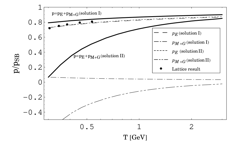
Figure 1: The solutions I and II for the optimal approximant, $p/p_{\mbox{\scriptsize{SB}}}$, as functions of $T$, when $\delta_{G}=\left(\delta_{E}\right)_{\overline{\mbox{\scriptsize{MS}}}}=0$. ($p_{\mbox{\scriptsize{SB}}}$ is the Stefan-Boltzmann pressure.) The optimized long-distance pressure $p_{M+G}$ and the short-distance pressure $p_{E}$ are also separately shown. The circles are the predictions of the lattice calculations.

In Fig. 1, we present the solutions I and II against $T$. The results are normalized by the Stefan-Boltzmann pressure $p_{\mbox{\scriptsize{SB}}}$ (cf. Eq. (21)). Also shown are the optimized long-distance pressure $p_{M+G}$ and the short-distance pressure $p_{E}$. The circles are the predictions of the lattice calculations [11] (see Ref. 9) for details.) From the figures we see that i) for the solution II, $p_{M+G}<0$ and ii) the solution I gives better agreement with the lattice result. From these observations, in the following, we adopt the solution I as the better candidate for the optimal approximant.

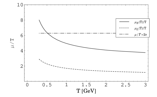
Figure 2: The optimized $\mu_{M+G}$, $\mu_{L}(T)$, and $\mu_{E}$, $\mu_{S}(T)$, for $\delta_{G}=\left(\delta_{E}\right)_{\overline{\mbox{\scriptsize{MS}}}}=0$ as functions of $T$. The dot-dashed lines shows the traditional choice $\mu=2\pi T$.

In Fig. 2 the optimized $\mu_{M+G}$, $\mu_{L}(T)$, and $\mu_{E}$, $\mu_{S}(T)$, are shown against $T$. The dot-dashed lines shows the traditional choice $\mu=2\pi T$. The ratios $\mu_{S}(T)/T$ and $\mu_{L}(T)/T$ decrease monotonically with $T$: The ratio $\mu_{S}(T)/2\pi T$ is larger than 1 at $T=0.3$ GeV, $\simeq 1$ at $T=0.5$ GeV and becomes smaller than 1 for $T>0.5$ GeV. $\mu_{L}(T)$ is smaller than $\mu_{S}(T)$ and $\mu_{L}(T)/\mu_{S}(T)\simeq 0.31\sim 0.36$ in the range shown in the figure. This is in accord with an intuition: The scale $\mu_{E}$ that governs the physics in the hard region, being of $O(T)$, is larger than the scale $\mu_{G+M}$ in the soft region.

Fig. 3 depicts the optimized $\beta_{2}$, $\beta_{2S}(T)$, against $T$. The dashed line shows $\beta_{2}=(\beta_{2})_{\overline{\mbox{\scriptsize{MS}}}}$. $\beta_{2S}(T)$ monotonically decreases with $T$ crossing the $\overline{\mbox{MS}}$ value at $T\simeq 0.5$ GeV. We note that Eq. (5) tells us that increase (decrease) in $\beta_{2}$ acts as increasing (decreasing) $\alpha_{s}$, the same effect as arising from decreasing (increasing) $\mu$. Then, we suspect that, if we fix $\beta_{2}$ to $\left(\beta_{2}\right)_{\overline{\mbox{\scriptsize{MS}}}}$ and vary only $\mu$, we obtain much smaller (larger) optimized $\mu_{E}$ for $T\lesssim 0.5$ ($T\gtrsim 0.5$) GeV. Thus, we expect that the optimized $\mu_{E}$ tends to $2\pi T$. It is amazing to note that, at $T\sim 0.5$ GeV, $\mu_{S}(T)$ and $\beta_{2S}(T)$ are close to the traditional choice $\mu=2\pi T$ and the $\overline{\mbox{MS}}$ value, respectively.

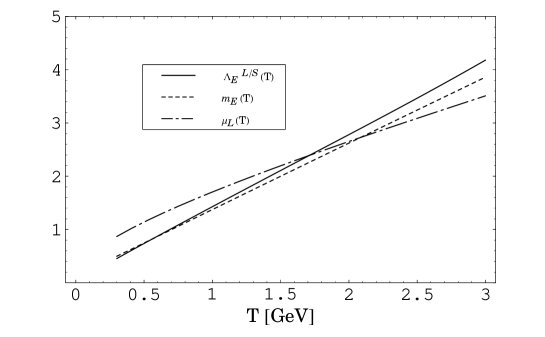
Figure 4: The optimized $\Lambda_{E}$, $\Lambda_{E}^{L/S}(T)$, and $m_{E}$ as functions of $T$. For reference, the optimized $\mu_{M+G}$, $\mu_{L}(T)$, is also shown.

In Fig. 4, we show the optimized $\Lambda_{E}$, $\Lambda_{E}^{L/S}(T)$, and $m_{E}(T)$ against $T$. For reference $\mu_{L}(T)$ in Fig. 2 is also shown again. We see that $\Lambda_{E}^{L/S}(T)\sim m_{E}(T)\sim\mu_{L}(T)\>(<\mu_{S}(T))$. This is not in accord with an intuitive expectation $\mu_{M+G}<\Lambda_{E}<\mu_{E}$. However, as seen at the end of §3, when $\mu_{M+G}$, $\mu_{E}$, and $\beta_{2}$ are fixed to their respective optimized values, the pressure $p$ does not depend on $\Lambda_{E}$.

In Fig. 5, we show the pressure $p$ at $T=0.5$ GeV near the optimized values of $\alpha_{s}^{E}\simeq\alpha_{s}^{S}(T)$, $\alpha_{s}^{M+G}\simeq\alpha_{s}^{L}(T)$, $\beta_{2}\simeq\beta_{2S}(T)$ and $\Lambda_{E}\simeq\Lambda_{E}^{L/S}(T)$. In Fig. 5 (a), we show the behavior of $p$ against $\alpha_{s}^{S}$, when other quantities, $\alpha_{s}^{M+G}$, $\beta_{2}$ and $\Lambda_{E}$ are fixed to the respective optimized values. The arrow indicates the optimized value of $\alpha_{s}^{E}$. Similarly, Figs. 5 (b) and (c) show the dependencies of $p$ on $\alpha_{s}^{M+G}$ and on $\beta_{2}$, respectively. From Fig. 5(c), we see that $p$ depends on $\beta_{2}$ only weakly. As has been repeatedly pointed out, $p$ does not depend on $\Lambda_{E}$, when $\alpha_{s}^{E}$, $\alpha_{s}^{M+G}$ and $\beta_{2}$ are fixed to the respective optimized values.

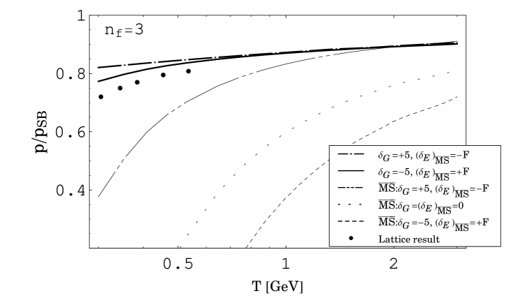
Figure 6: Optimal approximants (the solutions I) for $p/p_{\mbox{\scriptsize{SB}}}$ as functions of $T$ for various values of $\delta_{G}$ and $\left(\delta_{E}\right)_{\overline{\mbox{\scriptsize{MS}}}}$. Within the ranges, (16) and (25), of $(\delta_{G},\left(\delta_{E}\right)_{\overline{\mbox{\scriptsize{MS}}}})$, $(\delta_{G},\left(\delta_{E}\right)_{\overline{\mbox{\scriptsize{MS}}}})=(+5,-F)$, yields the maximum $p/p_{\mbox{\scriptsize{SB}}}$ (dot-dashed line) while $(\delta_{G},\left(\delta_{E}\right)_{\overline{\mbox{\scriptsize{MS}}}})=(-5,+F)$ yields the minimum one (solid line). For comparison, the lattice results and the $\overline{\mbox{MS}}$ results are also shown. Displayed $\overline{\mbox{MS}}$ results are the maximum one ${[}(\delta_{G},\left(\delta_{E}\right)_{\overline{\mbox{\scriptsize{MS}}}})=(+5,-F){]}$, within the ranges (16) and (25), the minimum one ${[}(\delta_{G},\left(\delta_{E}\right)_{\overline{\mbox{\scriptsize{MS}}}})=(-5,+F){]}$ and the one with $\delta_{G}=\left(\delta_{E}\right)_{\overline{\mbox{\scriptsize{MS}}}}=0$.

In Fig. 6, we present the optimal approximants for p, when the unknown constants $\left(\delta_{E}\right)_{\overline{\mbox{\scriptsize{MS}}}}$ and $\delta_{G}$ are varied. Within the ranges, (16) and (25), of the unknown constants, $(\delta_{G},\left(\delta_{E}\right)_{\overline{\mbox{\scriptsize{MS}}}})=(+5,-F)$ yields the maximum $p/p_{\mbox{\scriptsize{SB}}}$, while $(\delta_{G},\left(\delta_{E}\right)_{\overline{\mbox{\scriptsize{MS}}}})=(-5,+F)$ yields the minimum $p/p_{\mbox{\scriptsize{SB}}}$. For comparison, the $\overline{\mbox{MS}}$ results are also shown. From the figure, we see as a bonus that the resultant optimal approximants depend rather weakly on $\delta_{G}$ and $\left(\delta_{E}\right)_{\overline{\mbox{\scriptsize{{MS}}}}}$. Our results are substantially improved when compared to the $\overline{\mbox{MS}}$ results. Taking into account that the lattice results should be taken within an error of $10-15$ %, our results are well compatible with the lattice results.

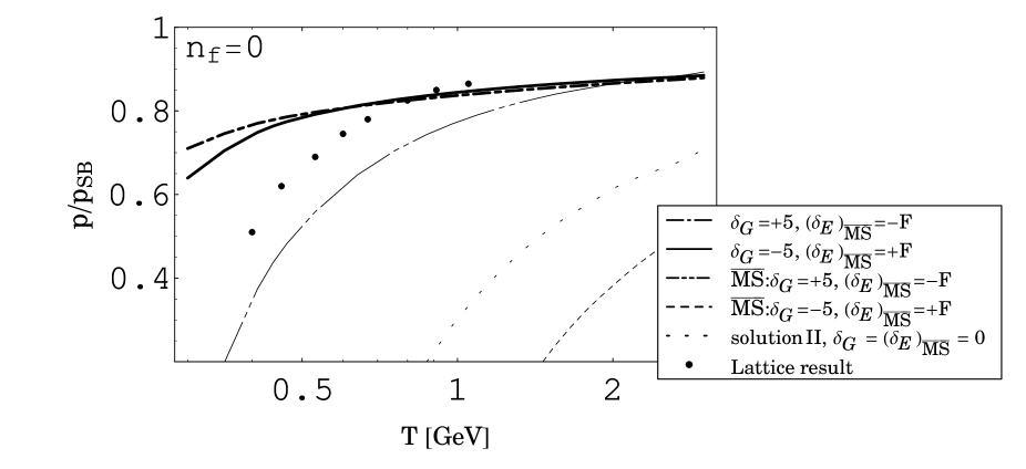
Figure 7: Analogous to Fig. 6 but with $n_{f}=0$. The solution II for $\delta_{G}=\left(\delta_{E}\right)_{\overline{\mbox{\scriptsize{{MS}}}}}=0$ is also shown.

Finally, in Fig. 7, we depicts the optimal approximants (solutions I) for the case of pure glue QCD ($n_{f}=0$). For comparison, the solution II for $\delta_{G}=\left(\delta_{E}\right)_{\overline{\mbox{\scriptsize{MS}}}}=0$ is also shown. Same comments as for the $n_{f}=3$ case applies here. For $\delta_{G}=\left(\delta_{E}\right)_{\overline{\mbox{\scriptsize{MS}}}}=0$, the $\overline{\mbox{MS}}$ result accidentally coincides with the solution II with high precision. Although the results are substantially improved when compared to the $\overline{\mbox{MS}}$ results (except for the case of $(\delta_{G},\left(\delta_{E}\right)_{\overline{\mbox{\scriptsize{MS}}}})=(+5,-F)$), agreement with the lattice results are less than that for the realistic case of $n_{f}=3$.

5 Discussion and Conclusion

The QCD pressure $p$ has been computed within the improved perturbation theory using the $\overline{\mbox{MS}}$ renormalization scheme, up to and including the $O(g^{6}_{s}\ln(1/g_{s}))$ and part of the $O(g^{6}_{s})$ terms. The truncated perturbation series for $p$ does not reconcile with the relatively low $T$ lattice results. As has been mentioned in §1, various approaches are proposed for improving the perturbative pressure $p$. Each approach performs a sort of resummation on the basis of respective philosophy. In this paper we add one more to them.

We have applied the Principles of Minimal Sensitivity (PMS) criterion to $p$. This is not new, but in Ref. 6), among other things, the PMS criterion has already been applied to $p$. However, as has been mentioned in §3, application is not made in a consistent manner. Meanwhile, an important observation is made in Ref. 9): The contributions to $p$ from the hard and soft energy regions, $p_{E}$ and $p_{M+G}$, are separately physical quantities. On the basis of this fact, we have applied the PMS criterion to $p_{E}$ and $p_{M+G}$ separately. For determining the factorization scale $\Lambda_{E}$, which separates hard and soft scales, we also adopt the minimal sensitivity criterion.

We have found that the optimal approximants are significantly improved when compared to the $\overline{\mbox{MS}}$ results. Especially, for the realistic case of $n_{f}=3$, agreement between our approximants and the lattice results is satisfactory. Moreover, we have found that, when compared to the $\overline{\mbox{MS}}$ results, the dependence of the approximants on the unknown terms of $O(g_{s}^{6})$ is rather weak. On the other hand, for the case of $n_{f}=0$, although the results are substantially improved, agreement with the lattice results are poorer than that for the $n_{f}=3$ case.

Further improvement may be expected if we perform the Padé type resummation starting from the optimal approximants obtained here, which is outside the scope of this paper.

Appendix A: Running Couplant

The relation between the three-loop running couplants $\alpha_{s}(\mu_{0},(\beta_{2})_{\overline{\mbox{\scriptsize{MS}}}})$ and
$\alpha_{s}(\mu,\beta_{2})$ is obtained by integrating the following two equations (cf. Eq. (7)),

$$\mu\frac{\partial\alpha_{s}}{\partial\mu} = \beta^{(3)}(\alpha_{s})\,,$$ (A.1)

$$\frac{\partial\alpha_{s}}{\partial\beta_{2}} = \gamma_{2}^{(3)}(\alpha_{s})\,,$$ (A.2)

along a path ${\cal C}$ in a $(\ln\mu,\beta_{2})$-plane, which starts from the point $(\ln\mu_{0},(\beta_{2})_{\overline{\mbox{\scriptsize{MS}}}})$ and arrives at the point $(\ln\mu,\beta_{2})$. Because of the integrability condition $\partial\beta^{(3)}(\alpha_{s})/\partial\beta_{2}=\partial\gamma^{(3)}_{2}(\alpha_{s})/\partial\ln\mu$, one can use any path ${\cal C}$. For convenience, we choose ${\cal C}={\cal C}_{1}\oplus{\cal C}_{2}\oplus{\cal C}_{3}$ with ${\cal C}_{1}=(\ln\mu_{0},(\beta_{2})_{\overline{\mbox{\scriptsize{MS}}}})\to(\ln\mu_{M},(\beta_{2})_{\overline{\mbox{\scriptsize{MS}}}})$, ${\cal C}_{2}=(\ln\mu_{M},(\beta_{2})_{\overline{\mbox{\scriptsize{MS}}}})\to(\ln\mu_{M},\beta_{2})$ and ${\cal C}_{3}=(\ln\mu_{M},\beta_{2})\to(\ln\mu,\beta_{2})$. At the final stage, we take the limit $\mu_{M}\to+\infty$.

Integrating Eq. (A.1) along the path ${\cal C}_{1}$, we obtain

$$\beta_{0}\ln\left(\frac{\mu_{M}}{\mu_{0}}\right) = \frac{1}{\alpha_{sM}}-\frac{1}{\alpha_{s0}}+\frac{\beta_{1}}{\beta_{0}}\ln\left(\frac{\alpha_{sM}}{\alpha_{s0}}\right)-\frac{\beta_{1}}{2\beta_{0}}\ln\left(\frac{\beta_{0}+\beta_{1}\alpha_{sM}+\left(\beta_{2}\right)_{\overline{\mbox{\scriptsize{MS}}}}\alpha_{sM}^{2}}{\beta_{0}+\beta_{1}\alpha_{s0}+\left(\beta_{2}\right)_{\overline{\mbox{\scriptsize{MS}}}}\alpha_{s0}^{2}}\right)$$ (A.3)

$$-\frac{\beta_{1}^{2}-2\beta_{0}\left(\beta_{2}\right)_{\overline{\mbox{\scriptsize{MS}}}}}{2\beta_{0}^{2}}\left[G\left(\alpha_{sM},\left(\beta_{2}\right)_{\overline{\mbox{\scriptsize{MS}}}}\right)-G\left(\alpha_{s0},\left(\beta_{2}\right)_{\overline{\mbox{\scriptsize{MS}}}}\right)\right]\,,$$

where $\alpha_{s0}=\alpha_{s}(\mu_{0},(\beta_{2})_{\overline{\mbox{\scriptsize{MS}}}})$ and $\alpha_{sM}=\alpha_{s}\left(\mu_{M},\left(\beta_{2}\right)_{\overline{\mbox{\scriptsize{MS}}}}\right)$ and

$$G(x,y)=\frac{2\beta_{0}}{\sqrt{4\beta_{0}y-\beta_{1}^{2}}}\arctan\left(\frac{2xy+\beta_{1}}{\sqrt{4\beta_{0}y-\beta_{1}^{2}}}\right)\,.$$

Integration of Eq. (A.1) along the path ${\cal C}_{3}$ yields a similar equation for $\beta_{0}\ln(\mu/\mu_{M})$. Adding this to Eq. (A.3), we obtain the formula for $\beta_{0}\ln(\mu/\mu_{0})$, which includes, among others, $\alpha_{s}\left(\mu_{M},\left(\beta_{2}\right)_{\overline{\mbox{\scriptsize{MS}}}}\right)$ and $\alpha_{s}(\mu_{M},\beta_{2})$. From Eq. (A.2), we see that $\alpha_{s}(\mu_{M},(\beta_{2})_{\overline{\mbox{\scriptsize{MS}}}})=\alpha_{s}(\mu_{M},\beta_{2})+O(\alpha_{s}^{3})$. Substituting this for $\alpha_{s}(\mu_{M},(\beta_{2})_{\overline{\mbox{\scriptsize{MS}}}})$ in the formula obtained above and taking the limit $\mu_{M}\to+\infty$ ($\alpha_{s}(\mu_{M},\beta_{2})\to 0$), we see that the $O(\alpha_{s}^{3})$ term does not survive.

Thus, we finally obtain

$$\beta_{0}\ln\left(\frac{\mu}{\mu_{0}}\right) = \frac{1}{\alpha_{s}}-\frac{1}{\alpha_{s0}}+\frac{\beta_{1}}{\beta_{0}}\ln\left(\frac{\alpha_{s}}{\alpha_{s0}}\right)-\frac{\beta_{1}}{2\beta_{0}}\ln\left(\frac{\beta_{0}+\beta_{1}\alpha_{s}+\beta_{2}\alpha_{s}^{2}}{\beta_{0}+\beta_{1}\alpha_{s0}+\left(\beta_{2}\right)_{\overline{\mbox{\scriptsize{MS}}}}\alpha_{s0}^{2}}\right)$$ (A.4)

$$-\frac{\beta_{1}^{2}-2\beta_{0}\left(\beta_{2}\right)_{\overline{\mbox{\scriptsize{MS}}}}}{2\beta_{0}^{2}}\left[G\left(0,\left(\beta_{2}\right)_{\overline{\mbox{\scriptsize{MS}}}}\right)-G\left(\alpha_{s0},\left(\beta_{2}\right)_{\overline{\mbox{\scriptsize{MS}}}}\right)\right]$$

$$-\frac{\beta_{1}^{2}-2\beta_{0}\beta_{2}}{2\beta_{0}^{2}}[G(\alpha_{s},\beta_{2})-G(0,\beta_{2})]\,,$$

where $\alpha_{s}=\alpha_{s}(\mu,\beta_{2})$.

Figure 3: The optimized $\beta_{2}$, $\beta_{2S}(T)$, as a function of $T$. The dashed line shows $\beta_{2}=(\beta_{2})_{\overline{\mbox{\scriptsize{MS}}}}$.

Figure 5: The pressure $p$ near the optimized values of $\alpha_{s}^{E}$, $\alpha_{s}^{M+G}$ and $\beta_{2}$, when $T=0.5$ Gev. The arrows in Figs. (a), (b) and (c) indicate the optimized values of $\alpha_{s}^{E}$, $\alpha_{s}^{M+G}$ and $\beta_{2}$, respectively. Details are given in the text.

References

- [1] P. Arnold and C. Zhai, Phys. Rev. D 50, 7603 (1994); ibid. 51, 1906 (1995); C. Zhai and B. Kastening, ibid. 52, 7232 (1995); E. Braaten and A. Nieto, Phys. Rev. Lett. 76, 1417 (1996); Phys. Rev. D 53, 3421 (1996).
- [2] K. Kajantie, M. Laine, K. Rummukainen, and Y. Schröder, Phys. Rev. D 67, 105008 (2003).
- [3] A. Peshier, B. Kämpfer, O. P. Pavlenko, and G. Soff, Phys. Rev. D 54, 2399 (1996); P. Lévai and U. Heinz, Phys. Rev. C 57, 1879 (1998).
- [4] J.-P. Blaizot , E. Iancu, and A. Rebhan, Phys. Lett. B470, 181 (1999); Phys. Rev. Lett. 83, 2906 (1999); A. Peshier, Phys. Rev. D 63, 105004 (2001).
- [5] F. Karsch, A. Patkós, and P. Petreczky, Phys. Lett. B401, 69 (1997); J. O. Andersen and M. Strickland, Phys. Rev. D 64, 105012 (2001).
- [6] J.-P. Blaizot , E. Iancu, and A. Rebhan, Phys. Rev. D 68, 025011 (2003).
- [7] J. O. Andersen, E. Braaten, and M. Strickland, Phys. Rev. D 61, 014017 (2000); ibid. 61, 074016 (2000); J. O. Andersen, E. Petitgirard, and M. Strickland, ibid. 70, 045001 (2004).
- [8] B. Kastening, Phys. Rev. D 56, 8107 (1997); T. Hatsuda, ibid. 56, 8111 (1997).
- [9] G. Cvetic̆ and R. Kögerler, Phys. Rev. D 70, 114016 (2004); ibid. 66, 105009 (2002).
- [10] P. M. Stevenson, Phys. Rev. D 23, 2916 (1981).
- [11] F. Karsch, E. Laermann, and A. Peikert, Phys. Lett. B478, 447 (2000); F. Karsch, Nucl. Phys. A698, 199 (2002).