We derive the analytic continuation of the Mellin moments of deep inelastic structure functions at the next-to-next-to-leading order accuracy.

1 Introduction

Deep inelastic (lepton-hadron) scattering (DIS) is one of the best studied reactions now. It provides unique information about the structure of the hadrons and tests one of the most important predictions of perturbative QCD, the scale evolution of the structure functions (SF) [1]-[3].

The increasing accuracy of the DIS experiments demands more accurate theoretical predictions. Very recently the calculations of the 3-loop corrections to anomalous dimensions (AD) of Wilson operators have been performed in [4, 5] that leads to complete theoretical information needed to analyze inclusive DIS reactions at the next-to-next-to-leading order (NNLO) accuracy.

The results have been presented in the Bjorken $x$-space for the corresponding splitting functions and also in the momentum space (i.e. in $n$-space) for the anomalous dimensions themselves. Although the $x$-space results have been done in complete form, the results for the anomalous dimensions have been presented in the form of nested sums, which are correct only for even or odd values of moments and cannot be used, for example, to determine directly the exact values of various sum rules, which correspond in the nonsinglet case to the Mellin moments of structure functions at $n=1$.

Of course, the sum rules can be extracted directly by integration of the $x$-space results for the splitting functions (see, for example, [6]-[8]). However, it is convenient to have a proper representations for the SF Mellin moments, where the sum rules values can be obtained automatically at $n=1$.

Despite the sum rules, the correct $n$-space representations are important also to reconstruct the structure functions and/or parton distributions from their corresponding moments. In general, for the back Mellin transformation someone should know the Mellin moments for the complex $n$ values.

To study the structure functions at intermediate $x$ values, sometimes there are important only the integer values of the Mellin moments. It is the case, for example, for programs to fit DIS experimental data, which are based on the Bernstein and Jacobi polynomials (see [9] and [10, 11], respectively). The programs are based on the exact solution of the DGLAP evolution equations [12] in the momentum space and on the reconstruction of the DIS structure functions at the end of evolution with help of the orthogonal polynomials (see, for example, [13],[14] and [11], [15]-[17] for the Bernstein and Jacobi polynomials, respectively).

This procedure is simpler to compare with the numerical solution of the DGLAP equations in $x$-space, which is used usually in global fits of experimental data (see, for example, [18] and references therein). The simplicity leads to possibility to use only partial information about the DIS coefficient functions and/or anomalous dimensions. For example, the first NNLO analysis of $F_{2}$ and $F_{3}$ structure functions have been obtained in [16] and [17] just after the first several even and odd moments of the nonsinglet anomalous dimensions have been calculated in [19].

To have the analytic continuation it is important also to study a similarity between the DGLAP [12] and BFKL [20] equations in the framework of ${\mathcal{N}}=4$ Supersymmetric Yang-Mills (SYM) theory (see [21]). The analytic structure of the BFKL kernel [22] in this model gives the possibility to predict the eigenvalues of AD matrix at the first three orders of perturbation theory (see Refs. [23], [21] and [24], respectively, and discussions therein). At the first two orders the predictions have been checked by direct calculations in [25].

Following to the studies [26]-[29], it is possible to show that at small $x$ values the $Q^{2}$-evolution of DIS structure functions is described (see [30]) by the behavior of their moments with the “number” $n=1+\delta$ in the case of Regge-type asymptotics of SF, i.e., for example, $F_{2}(x)\stackrel{{\scriptstyle x\to 0}}{{\sim}}x^{-\delta}$. In this case the continuation of the SF moments to real $n$ numbers is already needed.

The analytical continuation has been already obtained in [31, 28] (see also some similar studies in [32]), for a quite simple set of the nested sums $S_{-a,b,c,...}(n)$ (hereafter $a,b,c,...$ are integer and positive) :

$$S_{-a,b,c,...}(n)~{}=~{}\sum^{n}_{k=1}\frac{(-1)^{k}}{k^{a}}\,S_{b,c,...}(k),~{}~{}$$ (1)

where

$$S_{b,c,...}(n)~{}=~{}\sum^{n}_{k=1}\frac{1}{k^{b}}\,S_{c,...}(k),~{}~{}S_{d}(n)~{}=~{}\sum^{n}_{k=1}\frac{1}{k^{d}}.$$ (2)

Such nested sums contribute to the NLO corrections to the anomalous dimensions and coefficient functions (see [3, 33, 31, 34]). At the NNLO level, the QCD anomalous dimensions and coefficient functions [4, 5, 35, 36] contain more complicated nested sums $S_{\pm a,\pm b,\pm c,...}(n)$ and their continuation is the main subject of the study.

We note that the set of the nested sums is not fully independent: there are a lot of relations between the nested sums (see, for example, [37] and references therein) and, as the basic ones, we can use for the NNLO anomalous dimensions only ones in Eq. (1) and the additional sum $S_{a,-b,c,...}(n)$. Thus, really it is necessary to apply the results of [31, 28] and to study only the sums $S_{a,-b,c,...}(n)$.

Note, however, that the form of the NNLO anomalous dimensions are quite cumbersome and the new representation containing the nested sums (1) and $S_{a,-b,c,...}(n)$ will be long, too. So, it is better to keep the original Moch-Vermaseren-Vogt (MVV) representations and to give the analytic continuation for each nested sum of the MVV results.

Thus, the purpose of this study is the extension of the procedure of the analytic continuation given in [31, 28] for the more complicated nested sums $S_{\pm a,\pm b,\pm c,...}(n)$, that needs to $n$-space representations for anomalous dimensions and coefficient functions, which should be correct for arbitrary $n$ values. Moreover, after continuation the $n$-space representations should have the form which is very close to the original one in [4, 5, 35, 36]. As a by product of the study we present the results for $n=1$ which are related with QCD sum rules.

The structure of the paper is a following. Section 2 contains the general information about the properties of DIS structure functions and about method to extract the results for coefficient functions and anomalous dimensions. In section 3 we reproduce the basic steps of the analytic continuation [31, 28]. Section 4 contains the results of the analytic continuation for all needed nested sums $S_{\pm a,\pm b,\pm c,...}(n)$. In sections 5 and 6 there are some examples of the application of the analytic continuated results. Conclusion contains a summary of our results. Appendices A and B contain the basic steps of the procedure of the analytic continuation of the nested sums to the integer and real/complex arguments, respectively.

2 Basic formulae

The optical theorem relates the DIS structure functions to the forward scattering amplitude of photon-nucleon scattering, $T_{\mu\nu}$, which has a time-ordered the product of two local electromagnetic currents, $j_{\mu}(x)$ and $j_{\nu}(z)$. After Fourier transformation to momentum space, the standard perturbative theory can be applied. The operator product expansion allows to expand this current product around the light-cone $(x-z)^{2}\sim 0$ into a series of local composite operators $O_{\mu_{1},...,\mu_{n}}$ of leading twist and spin $n$. The anomalous dimensions on matrix elements $<h|O_{\mu_{1},...,\mu_{n}}|h>=p_{\mu_{1},...,\mu_{n}}A_{n}(p^{2}/\mu^{2})$ of these operators govern the scale evolution of the structure functions, while the coefficient functions multiplying these matrix elements are calculable in perturbative QCD.

Thus, for the scalar structure functions $T_{i}$ $(i=2,L,3)$ of the forward scattering amplitude $T_{\mu\nu}$ we have

$$T_{i}(Q^{2}) = \sum_{n=0}^{\infty}\frac{1}{x^{n}}T_{i,n}(Q^{2}),$$

$$T_{i,n}(Q^{2}) = \sum_{k=NS,q,g}C^{k}_{i,n}(Q^{2}/\mu^{2},\alpha_{s})A^{k}_{n}(\mu^{2}),~{}~{}~{}~{}(i=2,3,L).$$ (3)

The Wilson operators $A^{k}_{n}(\mu^{2})$ denote the spin-averaged hadronic matrix elements and $C_{i}$ are the coefficient functions and the sum extends over the flavor non-singlet and singlet quark and gluon contributions.

In this way the Mellin moments of DIS structure functions can naturally be written in the parameters of the operator product expansion (here and below our $F_{3}$ structure function is equal to standard $xF_{3}$ function)

$$\frac{1+(-1)^{n}}{2}\,\int^{1}_{0}dxx^{n-2}F_{i}(x,Q^{2})~{}=~{}\sum_{k=NS,q,g}C^{k}_{i,n}(Q^{2}/\mu^{2},\alpha_{s})A^{k}_{n}(\mu^{2})~{}~{}~{}~{}(i=2,3,L)$$ (4)

for $F^{e(\mu)p}_{2,L}(x,Q^{2})$ in the electron(muon)-proton scattering and for $F^{\nu p+\overline{\nu}p}_{2}(x,Q^{2})$ and
$F^{\nu p-\overline{\nu}p}_{3}(x,Q^{2})$ in the (anti-)neutrino-proton scattering and

$$\frac{1-(-1)^{n}}{2}\,\int^{1}_{0}dxx^{n-2}F_{i}(x,Q^{2})=C^{NS}_{i,n}(Q^{2}/\mu^{2},\alpha_{s})A^{NS}_{n}(\mu^{2})~{}~{}~{}~{}(i=2,3)$$ (5)

for $F^{\nu p-\overline{\nu}p}_{2}(x,Q^{2})$ and $F^{\nu p+\overline{\nu}p}_{3}(x,Q^{2})$ in the (anti-)neutrino-proton scattering.

The difference in Eqs. (4) and (5) comes from the relations $F^{e(\mu)p}_{2,L}(-x)=F^{e(\mu)p}_{2,L}(x)$, $F^{\overline{\nu}p}_{2}(-x)=-F^{\nu p}_{2}(x)$ and $F^{\overline{\nu}p}_{3}(-x)=F^{\nu p}_{3}(x)$ based on the charge symmetry (see [39] and references therein).

From Eqs. (4) and (5) one can see that only even and odd moments of the structure functions can be calculated from the odd (even) coefficients of the expansion of the corresponding functions $T_{2}$, $T_{L}$ and $xT_{3}$.

Thus, when we used $x$-space splitting functions coming in the forward scattering amplitude for full $x$-range, we neglect possible terms $\varphi(x)\pm\varphi(-x)$. This trivial analytic continuation in $x$-space leads at the lowest order of perturbation theory to similar trivial analytic continuation in $n$-space: we apply our results obtained at even or odd values to all integer one and after trivial extension to all real and/or complex $n$ values (see subsection 3.1). The nontrivial case comes at $n$-space starting at NLO approximation when nonplanar configurations start to contribute. The configurations lead to nonalternative nested sums which should be accurate continued to integer, real and/or complex results starting from even or odd ones.

Of course, after integration of the corresponding splitting-functions we obtain automatically this analytic continuation (see the review [40] and discussion therein). However, it is useful to have a procedure which allows to obtain directly the $n$-space results, completely extended to integer, real and/or complex results.

The coefficient functions and the anomalous dimensions are independent of a particular hadronic matrix element, so that it is standard to calculate partonic structure functions with external quarks and gluons in perturbation theory. In practice, this procedure reduces to the task of calculating the $n^{th}$ moment of all 4-point diagrams that contribute to $T_{\mu\nu}$ at a given order in perturbation theory (see [31, 34]).

To show this, it is better to use the Chetyrkin et al. “gluing” method [41]. The method allows to extract the contribution to coefficient function from a diagram by gluing its gluon legs by the additional propagator having the specific form: $q^{\mu_{1},...,\mu_{n}}/q^{2\alpha}$, where $q$ is gluon momentum and $\alpha$ is a special parameter.

Figure 1: The diagrams contributing to $T_{\mu\nu}$ for a gluon target. They should be multiplied by a factor of 2 because of the opposite direction of the fermion loop. The diagram (a) should be also doubled because of crossing symmetry.

As an example, we consider the diagrams on Fig. 1, which contribute to gluon parts of the coefficient functions and the anomalous dimensions.

The diagram (b) is less complicated nonplanar diagram, which contributes to coefficient functions. After gluing, the diagram obtains the new line containing $q^{\mu_{1},...,\mu_{n}}$.

The scalar Feynman integral having same topology has the following form ($k_{1}-k_{2}\equiv q$), when $\alpha=1$,

$$\int d^{D}k_{1}d^{D}k_{2}\frac{(k_{1}-k_{2})^{\mu_{1}}...(k_{1}-k_{2})^{\mu_{n}}}{k_{1}^{2}k_{2}^{2}(p-k_{1})^{2}(p-k_{2})^{2}(k_{1}-k_{2})^{2}}~{}=~{}\hat{N}\,I_{2}(n)\frac{p^{\mu_{1},...,\mu_{n}}}{{(p^{2})}^{5-D}}\,,$$ (6)

where $\hat{N}$ is a normalization factor and $D=4-2\epsilon$ is a space dimension.

When $D=4$, we have

$$I_{2}(n)~{}=~{}\delta^{0}_{n}\cdot 6\zeta(3)-\frac{1+(-1)^{n}}{n(n+1)}\,(1-\delta^{0}_{n})\,4S_{-2}(n),$$ (7)

where $\delta^{0}_{n}$ is the Kroneker symbol.

The example demonstrates the fact that the sum $S_{-1}(n)$ does not contribute to coefficient functions. The results for anomalous dimensions support the property. The absence of $S_{-1}(n)$ and also $\zeta(2)$ in results for coefficient functions and anomalous dimensions is sometimes very important result. For example, it helps very much in reconstruction of the eigenvalues of the NLO and NNLO anomalous dimensions of ${\mathcal{N}}=4$ Supersymmetric Yang-Mills theory (see [21] and [24], respectively). Moreover, the property can be a cross-check of the various calculations.

Note that $I_{2}(n)=0$ for odd $n$ values. It is easy to see from the symmetry property $k_{1}\leftrightarrow k_{2}$ of the Feynman integral (6) and up-down symmetry of gluing diagram on Fig. 1.

The zero values of the scalar coefficients $T_{i,n}(Q^{2})$ $(i=2,L,3)$ is the usual property of forward scattering amplitude $T_{\mu\nu}$.

As an example, we consider the diagrams on Fig. 1. Indeed, after gluing, the diagram (b) has the new line containing $q^{\mu_{1},...,\mu_{n}}$ and, from the symmetry $q\leftrightarrow-q$, the result for the diagram is zero for odd $n$ values.

The contribution of the diagram (a) is not zero but it is exactly cancelled at odd $n$ values by the contribution of its charge conjugated diagram. Indeed, the charge conjugated diagram coincides with the diagram (a) on Fig. 1 excepting gluons which propagate to opposite direction. Then, after gluing, the sum of the diagram (a) and its charge conjugated diagram contains the gluon propagator with numerator $\sim(1+(-1)^{n})q^{\mu_{1},...,\mu_{n}}$ and it is zero for odd $n$ values.

Thus, the analytic continuation is an important operation for DIS structure function because, using the procedure [31, 34] we calculate really another quantity: the forward scattering amplitude, and later we apply the obtained results for moments of the DIS structure functions. When, someone calculates a process directly, the analytic continuation is not so important property. For example, in the calculation of Feynman integrals with massive propagators it is convenient to use the back mass expansion [44], where the coefficients contain the considered nested sums. For the expansion, it is possible to use both: the original nested sums and/or its analytic continuation. The results do not depend of a concrete choice.

3 Procedure of analytic continuation

Here we would like to consider the analytic continuation procedure for the nested sums $S_{a,b,...}(n)$ Eq. (2) and $S_{-a,b,...}(n)$ Eq. (1). We will follow to the studies of Refs. [31, 28].

1. Consider the procedure of analytic continuation for the sums $S_{a}(n)$ and $S_{a,b,...}(n)$. Their form (2) is very convenient for the integer $n$ values and we should find representations which are useful for real/complex values of their argument.

1a. As the first example, let us to study the well known function:

$$S_{a}(n)~{}=~{}\sum^{n}_{j=1}\frac{1}{j^{a}}$$

for real and/or complex $n$ values.

Considering firstly the case $a\geq 2$, we have

$$S_{a}(n)~{}=~{}\biggl{[}\sum^{\infty}_{j=1}-\sum^{\infty}_{j=n}\biggr{]}\frac{1}{j^{a}}~{}=~{}S_{a}(\infty)-\sum^{\infty}_{l=0}\frac{1}{(l+n+1)^{a}}~{}\equiv~{}S_{a}(\infty)-\Psi_{a}(n+1),$$ (8)

where

$$S_{a}(\infty)~{}=~{}\zeta(a),~{}~{}~{}\Psi_{a}(n+1)~{}=~{}\frac{(-1)^{a}}{(a-1)!}\Psi^{(a-1)}(n+1),$$ (9)

$\zeta(a)$ is the Riemann zeta functions and $\Psi^{(a)}(n)$ is $a$-time derivative of the Euler $\Psi$-function, which is well known for any real and/or complex values of $n$.

For $a=1$ case the Eq. (8) transforms to

$$S_{1}(n)~{}=~{}\Psi(n+1)-\Psi(1)\,.$$ (10)

One can see that the basic step of analytic continuation is moving the variable $n$ from the upper limit of the sum to the sum argument. It is the basic step of our consideration here and below.

1b. Let us to continue with the function

$$S_{a,b,...}(n)~{}=~{}\sum^{n}_{j=1}\frac{1}{j^{a}}S_{b,...}(j)\,.$$

Repeating above analysis, we have got

$$S_{a,b,...}(n) = \biggl{[}\sum^{\infty}_{j=1}-\sum^{\infty}_{j=n}\biggr{]}\frac{1}{j^{a}}S_{b,...}(j)~{}=~{}S_{a,b,...}(\infty)-\sum^{\infty}_{l=0}\frac{1}{(l+n+1)^{a}}S_{b,...}(l+n+1)$$ (11)

$$= S_{a,b,...}(\infty)-\Psi_{a,b,...}(n+1),$$

where the function

$$\Psi_{a,b,...}(n+1)~{}=~{}\sum^{\infty}_{l=0}\frac{1}{(l+n+1)^{a}}S_{b,...}(l+n+1)$$

is also defined for any real and/or complex $n$ values.

From definition (2) we have that

$$S_{a,b}(\infty) = \zeta(a,b)+\zeta(a+b),$$

$$S_{a,b,c}(\infty) = \zeta(a,b,c)+\zeta(a+b,c)+\zeta(a,b+c)+\zeta(a+b+c),$$

$$S_{a,b,c,d}(\infty) = \zeta(a,b,c,d)+\zeta(a+b,c,d)+\zeta(a,b+c,d)+\zeta(a,b,c+d)$$ (12)

$$+ \zeta(a+b+c,d)+\zeta(a+b,c+d)+\zeta(a,b+c+d)+\zeta(a+b+c+d),$$

where $\zeta(a,b,c,d,...)$ are Eulier-Zagier alternative sums [45].

Note that sometimes (see, for example, [44]) the another definition of the nested sums $\tilde{S}_{\pm a,b,...}(n)$ is used, where

$$\tilde{S}_{\pm a,b,...}(n)~{}=~{}\sum^{n}_{k=1}\frac{(\pm 1)^{k}}{k^{a}}\,\tilde{S}_{b,...}(k-1),~{}~{}\tilde{S}_{\pm b}(n)~{}=~{}S_{\pm b}(n)~{}=~{}\sum^{n}_{k=1}\frac{(\pm 1)^{k}}{k^{b}}$$ (13)

and

$$\tilde{S}_{\pm a,b,...}(\infty) = \zeta(\pm a,b,...),$$ (14)

where $\zeta(\pm a,\pm b,\pm c,\pm d,...)$ are Eulier-Zagier nonalternative sums [45], when there is at least one negative argument.

The Eq. (12) comes from the one (14) and the relation between the nested sums $\tilde{S}_{\pm a,b,...}(n)$ and $S_{\pm a,b,...}(n)$:

$$S_{\pm a,b}(n) = \tilde{S}_{\pm a,b}(n)+\tilde{S}_{\pm(a+b)}(n),$$

$$S_{\pm a,b,c}(n) = \tilde{S}_{\pm a,b,c}(n)+\tilde{S}_{\pm(a+b),c}(n)+\tilde{S}_{\pm a,b+c}(n)+\tilde{S}_{\pm(a+b+c)}(n),$$

$$S_{\pm a,b,c,d}(n) = \tilde{S}_{\pm a,b,c,d}(n)+\tilde{S}_{\pm(a+b),c,d}(n)+\tilde{S}_{\pm a,b+c,d}(n)+\tilde{S}_{\pm a,b,c+d}(n)$$ (15)

$$+ \tilde{S}_{\pm(a+b+c),d}(n)+\tilde{S}_{\pm(a+b),c+d}(n)+\tilde{S}_{\pm a,b+c+d}(n)+\tilde{S}_{\pm(a+b+c+d)}(n).$$

2. Now we consider the procedure of analytic continuation for the sums $S_{-a}(n)$ and $S_{-a,b,...}(n)$, which come in consideration of the non-planar Feynman diagrams of forward scattering (see, for example, the Eqs. (6) and (7), the diagram (b) in Fig. 1 and discussions in Section 2).

2a. Let us firstly to consider the functions

$$S_{-a}(n)~{}=~{}\sum^{n}_{j=1}\frac{(-1)^{j}}{j^{a}}~{}=~{}-1+\frac{1}{2^{a}}-\frac{1}{3^{a}}+\frac{1}{4^{a}}-\frac{1}{5^{a}}+...~{},$$

which have the smooth behavior only for even or odd parts but not for all integer $n$ values, because there is a term $(-1)^{j}$. Indeed, we have the two different functions for even and odd $n$ values (see Fig. 2). Thus, we should determine firstly these two different functions for all integer $n$ values and later for real and complex ones. The functions, which have been analytically continuated from even and odd $n$ values, will be marked as $\overline{S}^{+}_{-a}(n)$ and $\overline{S}^{-}_{-a}(n)$, respectively.

Figure 2: The circles are represented the sums $S_{-2}(n)$ and $S_{-3}(n)$. The triangles show results for $\overline{S}_{-2}^{+}(n)$ and $\overline{S}_{-3}^{+}(n)$.

Let us to start with $\overline{S}^{+}_{-a}(n)$, which should be determine at its odd $n$ values. The consideration of $\overline{S}^{-}_{-a}(n)$ will be done in the following subsection.

By analogy with the subsection 1a, we have got

$$S_{-a}(n) = \biggl{[}\sum^{\infty}_{j=1}-\sum^{\infty}_{j=n}\biggr{]}\frac{(-1)^{j}}{j^{a}}~{}=~{}S_{-a}(\infty)-\sum^{\infty}_{l=0}\frac{(-1)^{l+n+1}}{(l+n+1)^{a}}$$ (16)

$$\equiv S_{-a}(\infty)-(-1)^{n}\Psi_{-a}(n+1),$$

where

$$S_{-1}(\infty) = \ln 2,~{}~{}S_{-a}(\infty)~{}=~{}\zeta(-a)~{}=~{}\left(2^{1-a}-1\right)\zeta(a),$$

$$\Psi_{-a}(n+1) = \sum^{\infty}_{l=0}\frac{(-1)^{l+1}}{(l+n+1)^{a}}~{}=~{}\frac{(-1)^{a}}{(a-1)!}\beta^{(a-1)}(n+1)$$ (17)

and $\beta^{(a)}(n)$ is $a$-time derivative of the $\beta(z)$-function:

$$\beta(z)=\frac{1}{2}\left[\Psi\left(\frac{1+z}{2}\right)-\Psi\left(\frac{z}{2}\right)\right],~{}~{}~{}\beta^{(a)}(z)=\frac{1}{2^{(a+1)}}\left[\Psi^{(a)}\left(\frac{1+z}{2}\right)-\Psi^{(a)}\left(\frac{z}{2}\right)\right],$$

which are well known for any real and/or complex values of its argument.

It is clearly seen that the nonsmooth $n$-dependence of the $S_{-a}(n)$ function is indicated as the term $(-1)^{n}$ in front of the smooth function $\Psi_{-a}(n+1)$. Then, the sum

$$(-1)^{n}S_{a}(n)~{}-~{}(-1)^{n}S_{-a}(\infty)=-\Psi_{-a}(n+1)$$

is smooth on $n$, and, thus, the function

$$\overline{S}^{+}_{-a}(n)~{}=~{}(-1)^{n}S_{-a}(n)~{}+~{}(1-(-1)^{n})S_{-a}(\infty)$$ (18)

is our needed result, because it is smooth on $n$ and coincides with the initial one $S_{-a}(n)$ for even $n$.

The results are presented on Fig. 2, where the functions $\overline{S}^{+}_{-2}(n)$ and $\overline{S}^{+}_{-3}(n)$ demonstrate their smooth $n$ behavior.

Note that

$$\overline{S}^{+}_{-a}(n)~{}=~{}S_{-a}(\infty)-\Psi_{-a}(n+1)$$ (19)

and, thus, it can be applied for real and/or complex $n$ values.

2b. By analogy with the previous subsection it is possible to show, that the continuation of the function $S_{-a}(n)$ from the odd $n$ values to all integer $n$ ones leads to the new function $\overline{S}^{-}_{-a}(n)$, which can be obtained replacing the factor $(-1)^{n}$ to the one $(-1)^{n+1}$ in the r.h.s. of Eqs. (18) and (19), i.e.

$$\overline{S}^{-}_{-a}(n)~{}=~{}(-1)^{n+1}S_{-a}(n)~{}+~{}(1-(-1)^{n+1})S_{-a}(\infty)~{}=~{}2S_{-a}(\infty)-\overline{S}^{+}_{-a}(n).$$ (20)

Note that the analytic continuation to the real and/or complex $n$-values gives

$$\overline{S}^{-}_{-a}(n)~{}=~{}S_{-a}(\infty)+\Psi_{-a}(n+1)$$ (21)

and, thus, the analytic continuated function $\overline{S}^{-}_{-a}(n)$ can be defined for real and/or complex $n$ values.

2c. By analogy with the above analysis for $S_{-a}(n)$ we able to consider the function $S_{-a,b,...}(n)$. We have got for its analytic continuation $\overline{S}^{+}_{-a,b,...}(n)$ as

$$\overline{S}^{+}_{-a,b,...}(n)~{}=~{}(-1)^{n}S_{-a,b,...}(n)~{}+~{}(1-(-1)^{n})S_{-a,b,...}(\infty),$$ (22)

which is defined for real and/or complex $n$ values, because

$$\overline{S}^{+}_{-a,b,...}(n)~{}=~{}S_{-a,b,...}(\infty)-\Psi_{-a,b,...}(n+1),$$ (23)

where

$$\Psi_{-a,b,...}(n+1)=\sum^{\infty}_{l=0}\frac{(-1)^{l+1}}{(l+n+1)^{a}}S_{b,...}(l+n+1).$$ (24)

In agreement with the analysis in the subsection 2b the analytic continuation $\overline{S}^{-}_{-a,b,...}(n)$ can be obtained similar to previous results: it is coincides with the Eq. (22) with the replacement $(-1)^{n}\to(-1)^{n+1}$, i.e.

$$\overline{S}^{-}_{-a,b,...}(n) = (-1)^{n+1}S_{-a,b,...}(n)~{}+~{}(1-(-1)^{n+1})S_{-a,b,...}(\infty),$$ (25)

$$= 2S_{-a,b,...}(\infty)-\overline{S}^{+}_{-a,b,...}(n)$$

and can be defined for real and/or complex $n$ values.

Indeed, for the analytic continuations $\overline{S}^{\pm}_{-a,b,...}(n)$ from even and odd $n$ values, respectively, to real and/or complex $n$ values, we have

$$\overline{S}^{\pm}_{-a,b,...}(n)~{}=~{}S_{-a,b,...}(\infty)\mp\Psi_{-a,b,...}(n+1).$$ (26)

Note that the functions $\overline{S}^{+}_{-a}(n)$ and $\overline{S}^{-}_{-a}(n)$ and also $\overline{S}^{+}_{-a,b,...}(n)$ and $\overline{S}^{-}_{-a,b,...}(n)$ are not independent each other (see Eqs. (21) and (25)).

From definition (1) we have that

$$S_{-a,b}(\infty)~{}=~{}\zeta(-a,b)+\zeta(-(a+b)),$$

$$S_{-a,b,c}(\infty)~{}=~{}\zeta(-a,b,c)+\zeta(-(a+b),c)+\zeta(-a,b+c)+\zeta(-(a+b+c)),$$

$$S_{-a,b,c,d}(\infty)~{}=~{}\zeta(-a,b,c,d)+\zeta(-(a+b),c,d)+\zeta(-a,b+c,d)+\zeta(-a,b,c+d)$$

$$\vspace{1cm}+\zeta(-(a+b+c),d)+\zeta(-(a+b),c+d)+\zeta(-a,b+c+d)+\zeta(-(a+b+c+d)).$$ (27)

2d. The functions $S_{-a}(n)$ and $S_{-a,b,...}(n)$ are related to the other popular ones (see [48, 26, 27]):

$$\tilde{S}(n)~{}=~{}S_{-2,1}(n),$$

$$S_{l}^{{}^{\prime}}(\frac{1}{2}n)~{}\equiv~{}S_{l}(\mbox{integer part of}\,\,\frac{n}{2})~{}=~{}2^{l-1}\Bigl{[}S_{l}(n)+S_{-l}(n)\Bigr{]}.$$

In agreement with the previous studies, these functions can be continuated from even to all integer $n$ values. They have the following form (see the second paper in [11])

$$\overline{S}^{{}^{\prime}+}_{2}(\frac{1}{2}n)~{}=~{}2S_{2}(n)+2\overline{S}^{+}_{-2}(n)~{}=~{}(-1)^{n}S^{{}^{\prime}}_{2}(n)+(1-(-1)^{n})\Bigl{[}2S_{2}(n)-\zeta(2)\Bigr{]},$$

$$\overline{S}^{{}^{\prime}+}_{3}(\frac{1}{2}n)~{}=~{}4S_{2}(n)+4\overline{S}^{+}_{-2}(n)~{}=~{}(-1)^{n}S^{{}^{\prime}}_{3}(n)+(1-(-1)^{n})\Bigl{[}4S_{2}(n)-3\zeta(3)\Bigr{]},$$

$$\overline{\tilde{S}}^{+}(n)~{}=~{}\overline{S}_{-2,1}^{+}(n)~{}=~{}(-1)^{n}\tilde{S}(n)-(1-(-1)^{n})\frac{5}{8}\zeta(3).$$ (28)

The continuation from odd to all integer $n$ values can be obtained by the replacement $(-1)^{n}\to(-1)^{n+1}$ in the r.h.s. of above equations.

The Eq. (28) and the replacement $(-1)^{n}\to(-1)^{n+1}$ in their r.h.s. correspond, respectively, to the “$+$” and “$-$” prescriptions (18), (20), (22) and (25).

4 More complicated cases

At the NLO approximations only the nonsmooth functions $S_{-a}(n)$ and $S_{-a,b,...}(n)$ contribute to the anomalous dimensions [26, 27] and the longitudinal coefficient functions [46]. At NNLO level the new functions

$$S_{a,-b,c,...}(n),~{}S_{-a,-b,c,...}(n),~{}S_{a,-b,-c,...}(n),~{}S_{-a,b,-c,...}(n),~{}S_{a,b,-c,...}(n)$$

start to play a role. In principle, the results of [4, 5] can be represented in the form where only the one new function $S_{a,-b,c,...}(n)$ contributes.

However, the original form of representations of the NNLO anomalous dimensions in [4, 5] seems to be most compact one and, so, it is better to keep it. In this case we should find the analytic continuations for all above sums.

Moreover, we consider also the sum $S_{-a,-b,-c,...}(n)$, which does not contribute to the NNLO corrections to the anomalous dimensions. However, it can contribute to future results [47] for the coefficient functions at NNLO level.

The derivation of the formulae is done in Appendix A. The final results for the analytic continuation from even $n$-values to integer ones has the form

$$\overline{S}^{+}_{-a,-b,...}(n) = S_{-a,-b,...}(n)~{}+~{}(1-(-1)^{n})S_{-b,...}(\infty)\,\biggl{[}S_{-a}(\infty)-S_{-a}(n)\biggr{]},$$ (29)

$$\overline{S}^{+}_{a,-b,...}(n) = (-1)^{n}S_{a,-b,...}(n)~{}+~{}(1-(-1)^{n})\biggl{[}S_{a,-b,...}(\infty)$$ (30)

$$-S_{-b,...}(\infty)\Bigl{(}S_{a}(\infty)-S_{a}(n)\Bigr{)}\biggr{]},$$

$$\overline{S}^{+}_{a,-b,-c,...}(n) = S_{a,-b,-c,...}(n)~{}+~{}(1-(-1)^{n})S_{-c,...}(\infty)\biggl{[}S_{a,-b}(\infty)-S_{a,-b}(n)$$ (31)

$$-S_{-b}(\infty)\Bigr{(}S_{a}(\infty)-S_{a}(n)\Bigr{)}\biggr{]},$$

$$\overline{S}^{+}_{-a,b,-c,...}(n) = S_{-a,b,-c,...}(n)~{}+~{}(1-(-1)^{n})\Biggl{[}\biggl{(}S_{b,-c,...}(\infty)-S_{b}(\infty)S_{-c,...}(\infty)\biggr{)}$$ (32)

$$\times\Bigl{(}S_{-a}(\infty)-S_{-a}(n)\Bigr{)}~{}+~{}S_{-c,...}(\infty)\biggr{(}S_{-a,b}(\infty)-S_{-a,b}(n)\biggr{)}\Biggr{]},$$

$$\overline{S}^{+}_{a,b,-c,...}(n) = (-1)^{n}S_{a,b,-c,...}(n)~{}+~{}(1-(-1)^{n})\Biggl{[}S_{a,b,-c,...}(\infty)$$ (33)

$$-\biggl{(}S_{b,-c,...}(\infty)-S_{b}(\infty)S_{-c,...}(\infty)\biggr{)}\Bigl{(}S_{a}(\infty)-S_{a}(n)\Bigr{)}$$

$$-S_{-c,...}(\infty)\biggr{(}S_{a,b}(\infty)-S_{a,b}(n)\biggr{)}\Biggr{]},$$

$$\overline{S}^{+}_{-a,-b,-c,...}(n) = (-1)^{n}S_{-a,-b,-c,...}(n)~{}+~{}(1-(-1)^{n})\Biggl{[}S_{-a,-b,-c,...}(\infty)$$ (34)

$$\hskip-42.67912pt-S_{-c,...}(\infty)\biggl{(}S_{-a,-b}(\infty)-S_{-a,-b}(n)-S_{-b}(\infty)\Bigl{(}S_{-a}(\infty)-S_{-a}(n)\Bigr{)}\biggr{)}\Biggr{]}.$$

We can see that the formulae are similar to ones presented in the previous section but they have little more complicated form.

As it was before, the analytic continuation from odd $n$ values to the integer ones can be done by replacement all terms $(-1)^{n}$ by ones $(-1)^{n+1}$, i.e.

$$\overline{S}^{-}_{-a,-b,...}(n) = S_{-a,-b,...}(n)~{}+~{}(1-(-1)^{n+1})S_{-b,...}(\infty)\,\biggl{[}S_{-a}(\infty)-S_{-a}(n)\biggr{]},$$ (35)

$$\overline{S}^{-}_{a,-b,...}(n) = (-1)^{n+1}S_{a,-b,...}(n)~{}+~{}(1-(-1)^{n+1})\biggl{[}S_{a,-b,...}(\infty)$$ (36)

$$-S_{-b,...}(\infty)\Bigl{(}S_{a}(\infty)-S_{a}(n)\Bigr{)}\biggr{]},$$

$$\overline{S}^{-}_{a,-b,-c,...}(n) = S_{a,-b,-c,...}(n)~{}+~{}(1-(-1)^{n+1})S_{-c,...}(\infty)\biggl{[}S_{a,-b}(\infty)-S_{a,-b}(n)$$ (37)

$$-S_{-b}(\infty)\Bigr{(}S_{a}(\infty)-S_{a}(n)\Bigr{)}\biggr{]},$$

$$\overline{S}^{-}_{-a,b,-c,...}(n) = S_{-a,b,-c,...}(n)~{}+~{}(1-(-1)^{n+1})\Biggl{[}\biggl{(}S_{b,-c,...}(\infty)-S_{b}(\infty)S_{-c,...}(\infty)\biggr{)}$$ (38)

$$\times\Bigl{(}S_{-a}(\infty)-S_{-a}(n)\Bigr{)}~{}+~{}S_{-c,...}(\infty)\biggr{(}S_{-a,b}(\infty)-S_{-a,b}(n)\biggr{)}\Biggr{]},$$

$$\overline{S}^{-}_{a,b,-c,...}(n) = (-1)^{n+1}S_{a,b,-c,...}(n)~{}+~{}(1-(-1)^{n+1})\Biggl{[}S_{a,b,-c,...}(\infty)$$ (39)

$$-\biggl{(}S_{b,-c,...}(\infty)-S_{b}(\infty)S_{-c,...}(\infty)\biggr{)}\Bigl{(}S_{a}(\infty)-S_{a}(n)\Bigr{)}$$

$$-S_{-c,...}(\infty)\biggr{(}S_{a,b}(\infty)-S_{a,b}(n)\biggr{)}\Biggr{]},$$

$$\overline{S}^{-}_{-a,-b,-c,...}(n) = (-1)^{n+1}S_{-a,-b,-c,...}(n)~{}+~{}(1-(-1)^{n+1})\Biggl{[}S_{-a,-b,-c,...}(\infty)$$ (40)

$$\hskip-42.67912pt-S_{-c,...}(\infty)\biggl{(}S_{-a,-b}(\infty)-S_{-a,-b}(n)-S_{-b}(\infty)\Bigl{(}S_{-a}(\infty)-S_{-a}(n)\Bigr{)}\biggr{)}\Biggr{]}.$$

As it was shown in the previous section, the “$+$” and “$-$” forms of analytic continuations are not independent from each other. Indeed, we have

$$\overline{S}^{-}_{-a,-b,...}(n) = \overline{S}^{+}_{-a,-b,...}(n)\ +\ 2\,(-1)^{n}\,S_{-b,...}(\infty)\biggl{[}S_{-a}(\infty)-S_{-a}(n)\biggr{]}$$ (41)

$$= \overline{S}^{+}_{-a,-b,...}(n)\ +\ 2\,S_{-b,...}(\infty)\biggl{[}S_{-a}(\infty)-\overline{S}^{+}_{-a}(n)\biggr{]},$$

$$\overline{S}^{-}_{a,-b,...}(n) = 2\,\biggl{[}S_{a,-b,...}(\infty)-S_{-b,...}(\infty)\Bigl{(}S_{a}(\infty)-S_{a}(n)\Bigr{)}\biggr{]}~{}-~{}\overline{S}^{+}_{a,-b,...}(n),$$ (42)

$$\overline{S}^{-}_{a,-b,-c,...}(n) = \overline{S}^{+}_{a,-b,-c,...}(n)\ +\ 2\,(-1)^{n}\,S_{-c,...}(\infty)\biggl{[}S_{a,-b}(\infty)-S_{a,-b}(n)$$ (43)

$$-S_{-b}(\infty)\Bigr{(}S_{a}(\infty)-S_{a}(n)\Bigr{)}\biggr{]}~{}=~{}\overline{S}^{+}_{a,-b,-c,...}(n)\ +\ 2\,S_{-c,...}(\infty)$$

$$\times\biggl{[}S_{a,-b}(\infty)-\overline{S}^{+}_{a,-b}(n)-S_{-b}(\infty)\Bigr{(}S_{a}(\infty)-S_{a}(n)\Bigr{)}\biggr{]},$$

$$\overline{S}^{-}_{-a,b,-c,...}(n) = \overline{S}^{+}_{-a,b,-c,...}(n)\ +\ 2\,(-1)^{n}\,\Biggl{[}\biggl{(}S_{b,-c,...}(\infty)-S_{b}(\infty)S_{-c,...}(\infty)\biggr{)}$$ (44)

$$\times\Bigl{(}S_{-a}(\infty)-S_{-a}(n)\Bigr{)}~{}+~{}S_{-c,...}(\infty)\biggr{(}S_{-a,b}(\infty)-S_{-a,b}(n)\biggr{)}\Biggr{]}$$

$$= \overline{S}^{+}_{-a,b,-c,...}(n)\ +\ 2\,\Biggl{[}\biggl{(}S_{b,-c,...}(\infty)-S_{b}(\infty)S_{-c,...}(\infty)\biggr{)}$$

$$\times\Bigl{(}S_{-a}(\infty)-\overline{S}^{+}_{-a}(n)\Bigr{)}~{}+~{}S_{-c,...}(\infty)\biggr{(}S_{-a,b}(\infty)-\overline{S}^{+}_{-a,b}(n)\biggr{)}\Biggr{]},$$

$$\overline{S}^{-}_{a,b,-c,...}(n) = 2\,\Biggl{[}S_{a,b,-c,...}(\infty)~{}-~{}\biggl{(}S_{b,-c,...}(\infty)-S_{b}(\infty)S_{-c,...}(\infty)\biggr{)}\Bigl{(}S_{a}(\infty)-S_{a}(n)\Bigr{)}$$ (45)

$$-S_{-c,...}(\infty)\biggr{(}S_{a,b}(\infty)-S_{a,b}(n)\biggr{)}\Biggr{]}-\overline{S}^{+}_{a,b,-c,...}(n),$$

$$\overline{S}^{-}_{-a,-b,-c,...}(n) = 2\,\Biggl{[}S_{-a,-b,-c,...}(\infty)-S_{-c,...}(\infty)\biggl{(}S_{-a,-b}(\infty)-S_{-a,-b}(n)$$ (46)

$$-S_{-b}(\infty)\Bigl{(}S_{-a}(\infty)-S_{-a}(n)\Bigr{)}\biggr{)}\Biggr{]}-\overline{S}^{+}_{-a,-b,-c,...}(n)$$

$$= 2\,\Biggl{[}S_{-a,-b,-c,...}(\infty)-S_{-c,...}(\infty)\biggl{(}S_{-a,-b}(\infty)-\overline{S}^{+}_{-a,-b}(n)$$

$$-S_{-b}(\infty)\Bigl{(}S_{-a}(\infty)-\overline{S}^{+}_{-a}(n)\Bigr{)}\biggr{)}\Biggr{]}-\overline{S}^{+}_{-a,-b,-c,...}(n).$$

Similar to Eq. (25), the relations between the “$+$” and “$-$” forms of analytic continuations have smooth $n$-dependence.

The analytic continuation to real and/or complex $n$ values can be easy obtained from above formulae. It has the form (see Appendix B for details):

$$\overline{S}_{-a,-b,...}^{+}(n) = S_{-a,-b,...}(\infty)-\Psi_{a,-b,...}(n+1)$$ (47)

$$+ S_{-b,...}(\infty)\Bigl{[}\Psi_{a}(n+1)-\Psi_{-a}(n+1)\Bigr{]},$$

$$\overline{S}_{a,-b,...}^{+}(n) = S_{a,-b,...}(\infty)-\Psi_{-a,-b,...}(n+1)$$ (48)

$$+ S_{-b,...}(\infty)\Bigl{[}\Psi_{-a}(n+1)-\Psi_{a}(n+1)\Bigr{]},$$

$$\overline{S}_{a,-b,-c,...}^{+}(n) = S_{a,-b,-c,...}(\infty)-\Psi_{a,-b,-c,...}(n+1)$$ (49)

$$+ S_{-c,...}(\infty)\biggl{[}\Psi_{-a,-b}(n+1)-\Psi_{a,-b}(n+1)$$

$$- S_{-b}(\infty)\Bigl{(}\Psi_{a}(n+1)-\Psi_{-a}(n+1)\Bigr{)}\biggr{]},$$

$$\overline{S}_{-a,b,-c,...}^{+}(n) = S_{-a,b,-c,...}(\infty)-\Psi_{a,b,-c,...}(n+1)$$ (50)

$$+ \Bigl{[}S_{b,-c,...}(\infty)-S_{b}(\infty)S_{-c,...}(\infty)\Bigr{]}\Bigl{(}\Psi_{a}(n+1)-\Psi_{-a}(n+1)\Bigr{)}$$

$$+ S_{-c,...}(\infty)\Bigl{(}\Psi_{a,b}(n+1)-\Psi_{-a,b}(n+1)\Bigr{)},$$

$$\overline{S}_{a,b,-c,...}^{+}(n) = S_{a,b,-c,...}(\infty)-\Psi_{-a,b,-c,...}(n+1)$$ (51)

$$+ \Bigl{[}S_{b,-c,...}(\infty)-S_{b}(\infty)S_{-c,...}(\infty)\Bigr{]}\Bigl{(}\Psi_{-a}(n+1)-\Psi_{a}(n+1)\Bigr{)}$$

$$+ S_{-c,...}(\infty)\Bigl{(}\Psi_{-a,b}(n+1)-\Psi_{a,b}(n+1)\Bigr{)},$$

$$\overline{S}_{-a,-b,-c,...}^{+}(n) = S_{-a,-b,-c,...}(\infty)-\Psi_{-a,-b,-c,...}(n+1)$$ (52)

$$+ S_{-c,...}(\infty)\biggl{[}\Psi_{-a,-b}(n+1)-\Psi_{a,-b}(n+1)$$

$$+ S_{-b}(\infty)\Bigl{(}\Psi_{a}(n+1)-\Psi_{-a}(n+1)\Bigr{)}\biggr{]},$$

where

$$\Psi_{a,-b,...}(n+1) = \sum_{l=0}^{\infty}\frac{1}{(l+n+1)^{a}}\overline{S}_{-b,...}^{+}(l+n+1),$$ (53)

$$\Psi_{-a,-b,...}(n+1) = \sum_{l=0}^{\infty}\frac{(-1)^{l+1}}{(l+n+1)^{a}}\overline{S}_{-b,...}^{+}(l+n+1),$$ (54)

$$\Psi_{a,-b,-c,...}(n+1) = \sum_{l=0}^{\infty}\frac{1}{(l+n+1)^{a}}\overline{S}_{-b,-c,...}^{+}(l+n+1),$$ (55)

$$\Psi_{a,b,-c,...}(n+1) = \sum_{l=0}^{\infty}\frac{1}{(l+n+1)^{a}}\overline{S}_{b,-c...}^{+}(l+n+1),$$ (56)

$$\Psi_{-a,b,-c,...}(n+1) = \sum_{l=0}^{\infty}\frac{(-1)^{l+1}}{(l+n+1)^{a}}\overline{S}_{b,-c,...}^{+}(l+n+1),$$ (57)

$$\Psi_{-a,-b,-c,...}(n+1) = \sum_{l=0}^{\infty}\frac{(-1)^{l+1}}{(l+n+1)^{a}}\overline{S}_{-b,-c,...}^{+}(l+n+1).$$ (58)

So, now the functions $\overline{S}_{-a,-b,...}^{+}(n)$, $\overline{S}_{a,-b,...}^{+}(n)$, $\overline{S}_{a,-b,-c,...}^{+}(n)$, $\overline{S}_{-a,-b,-c,...}^{+}(n)$, $\overline{S}_{-a,b,-c,...}^{+}(n)$ and $\overline{S}_{a,b,-c,...}^{+}(n)$ are well defined for the real and/or complex $n$ values.

The results for the analytic continuation to real and/or complex $n$ values of the corresponding functions $\overline{S}_{-a,-b,...}^{-}(n)$, $\overline{S}_{a,-b,...}^{-}(n)$, $\overline{S}_{a,-b,-c,...}^{-}(n)$, $\overline{S}_{-a,-b,-c,...}^{-}(n)$, $\overline{S}_{-a,b,-c,...}^{-}(n)$ and $\overline{S}_{a,b,-c,...}^{-}(n)$ can be found taking together Eqs. (41)-(46) and (47)-(58).

5 Simple example

As some examples we will study analytic continuation of the nonsinglet parts of NLO and NNLO anomalous dimensions and NNLO Wilson coefficient functions. The NLO nonsinglet anomalous dimension $\gamma^{(1),\pm}_{NS}(n)$ will be considered in this section and other variables will be studied in the following one.

Here we will follow to the form of $\gamma^{(1)\pm}_{NS}$ given in perfect Yndurain book [48]:

$$\gamma^{(1),\pm}_{NS}(n)~{}=~{}\frac{64}{9}\Bigl{[}A_{1}(n)~{}+~{}A_{2}(n)~{}\pm~{}A_{3}(n)\Bigr{]},$$ (59)

where

$$A_{1}(n) = S_{3}(n)~{}-~{}4S_{2}(n)\Bigl{[}2S_{1}(n)-\frac{1}{n(n+1)}+\frac{21}{8}\Bigr{]}$$ (60)

$$+ S_{1}(n)\Bigl{[}\frac{67}{2}+\frac{4(2n+1)}{n^{2}(n+1)^{2}}\Bigr{]}~{}-~{}\frac{63}{16}~{}-~{}\frac{151n^{4}+260n^{3}+96n^{2}+3n+10}{4n^{3}(n+1)^{3}}$$

$$+ f\Bigl{[}S_{2}(n)-\frac{5}{3}S_{1}(n)+\frac{11n^{2}+5n-3}{6n^{2}(n+1)^{2}}+\frac{1}{8}\Bigr{]},$$

$$A_{2}(n) = S_{-3}(n)-2S_{-2,1}(n)+S_{-2}(n)\Bigl{[}2S_{1}(n)-\frac{1}{n(n+1)}\Bigr{]},$$ (61)

$$A_{3}(n) = \frac{2n^{2}+2n+1}{2n^{3}(n+1)^{3}}$$ (62)

and $f$ is the number of active quarks.

Formally, the difference between the anomalous dimensions $\gamma^{(1),+}_{NS}$ and $\gamma^{(1),-}_{NS}$ is proportional to function $A_{3}(n)$. After the analytic continuation from even and odd $n$ values for the AD $\gamma^{(1),+}_{NS}$ and $\gamma^{(1),-}_{NS}$, respectively, the situation changes essentially.

Indeed, in agreement with the previous section to extend the results (59) to integer, real and/or complex $n$ values we can use “$+$” and “$-$” prescriptions (18)-(27) for the anomalous dimensions $\gamma^{(1),+}_{NS}$ and $\gamma^{(1),-}_{NS}$, respectively,

Then, we have the analytically continuated anomalous dimensions in the form

$$\gamma^{(1),\pm}_{NS}(n)~{}=~{}\frac{64}{9}\Bigl{[}A_{1}(n)~{}+~{}\overline{A}_{2}^{\pm}(n)~{}\pm~{}A_{3}(n)\Bigr{]},$$ (63)

where

$$\overline{A}_{2}^{\pm}(n)~{}=~{}\overline{S}_{-3}^{\pm}(n)-2\overline{S}_{-2,1}^{\pm}(n)+\overline{S}_{-2}^{\pm}(n)\Bigl{[}2S_{1}(n)-\frac{1}{n(n+1)}\Bigr{]}.$$ (64)

1. It is useful to see the difference between anomalous dimensions $\gamma^{(1)-}_{NS}$ and $\gamma^{(1)+}_{NS}$ :

$$\gamma^{(1)-}_{NS}~{}-~{}\gamma^{(1)+}_{NS}~{}=~{}\frac{64}{9}\Bigl{[}\hat{A}_{2}(n)~{}-~{}2A_{3}(n)\Bigr{]},$$ (65)

where

$$\hat{A}_{2}(n)~{}=~{}\overline{A}_{2}^{-}(n)-\overline{A}_{2}^{+}(n)~{}=~{}\hat{S}_{-3}(n)-2\hat{S}_{-2,1}(n)-\hat{S}_{-2}(n)\Bigl{[}2S_{1}(n)-\frac{1}{n(n+1)}\Bigr{]}$$ (66)

and

$$\hat{S}_{-a}(n) = \overline{S}_{-a}^{-}(n)-\overline{S}_{-a}^{+}(n)~{}=~{}2\Bigl{(}S_{-a}(\infty)-\overline{S}_{-a}^{+}(n)\Bigr{)}~{}=~{}2(-1)^{n}\Bigl{(}S_{-a}(\infty)-S_{-a}(n)\Bigr{)},$$

$$\hat{S}_{-a,b}(n) = \overline{S}_{-a,b}^{-}(n)-\overline{S}_{-a,b}^{+}(n)~{}=~{}2\Bigl{(}S_{-a,b}(\infty)-\overline{S}_{-a,b}^{+}(n)\Bigr{)}$$ (67)

$$= 2(-1)^{n}\Bigl{(}S_{-a,b}(\infty)-S_{-a,b}(n)\Bigr{)}.$$

For the several first $n$ values the results for anomalous dimensions $\gamma^{(1)-}_{NS}$ and $\gamma^{(1)+}_{NS}$ and their difference are give in the Table 1. One can see, that the ratio of $(\gamma^{(1)+}_{NS}-\gamma^{(1)-}_{NS})/\gamma^{(1)+}_{NS}$, which is equal to 1 at $n=1$, is very small already started with $n\geq 2$.

Table 1: the results for anomalous dimensions $\gamma^{(1)-}_{NS}$ and $\gamma^{(1)+}_{NS}$ and their difference at the first four even $n$ values.

$n$	2	4	6	8
$\gamma^{(1)+}_{NS}$	77.70	133.25	164.26	186.68
$\gamma^{(1)+}_{NS}-\gamma^{(1)-}_{NS}$	1.335 $\cdot 10^{-1}$	4.6$\cdot 10^{-3}$	4$\cdot 10^{-4}$	7$\cdot 10^{-5}$
$\frac{\gamma^{(1)+}_{NS}-\gamma^{(1)-}_{NS}}{\gamma^{(1)+}_{NS}}$	1.87$\cdot 10^{-3}$	3.9$\cdot 10^{-5}$	3$\cdot 10^{-6}$	4$\cdot 10^{-7}$

Considering $1/n$ expansion (see [26, 27]), which is the very good approximation starting with $n=4$, we have:

$$\hat{A}_{2}(n)~{}=~{}\frac{2}{n^{4}}\left(1-\frac{2}{n}+\frac{13}{2n^{2}}\right)+O\left(\frac{1}{n^{7}}\right),~{}~{}~{}A_{3}(n)~{}=~{}\frac{1}{n^{4}}\left(1-\frac{2}{n}+\frac{7}{2n^{2}}\right)+O\left(\frac{1}{n^{7}}\right)$$ (68)

and, thus,

$$\gamma^{(1)-}_{NS}~{}-~{}\gamma^{(1)+}_{NS}~{}=~{}\frac{128}{3}\frac{1}{n^{6}}+O\left(\frac{1}{n^{7}}\right)$$ (69)

It is possible to show the similar property for the NNLO anomalous dimensions, i.e. $(\gamma^{(2)+}_{NS}(n)-\gamma^{(2)-}_{NS}(n))/\gamma^{(2)+}_{NS}(n)\ll 1$ for $n\geq 2$. The property was important for fits of experimental data of $xF_{3}$ structure functions at NNLO approximation (see first three papers in [17]). At that time, the results for the anomalous dimension $\gamma^{(2)-}_{NS}(n)$ have been unknown and it has been replaced by $\gamma^{(2)+}_{NS}(n)$.

2. It is interesting to see the values of so-called Adler and Gottfried sum rules, $I_{3}^{-}$ and $I_{2}^{+}$, respectively, which have the following form at the first three orders of perturbation theory ($l=2,3$):

$$I_{l}^{\pm} = N_{l}^{\pm}\,C_{l}^{\pm}(\overline{\alpha}_{s}(Q^{2}))\,A^{\pm}(\overline{\alpha}_{s}(Q^{2})),$$

$$C_{l}^{\pm}(\overline{\alpha}_{s}(Q^{2})) = 1+\overline{\alpha}_{s}(Q^{2})\,B_{l,NS}^{(1)}(n=1)+\overline{\alpha}_{s}^{2}(Q^{2})\,B_{l,NS}^{(2),\pm}(n=1)+O\Bigl{(}\overline{\alpha}_{s}^{3}(Q^{2})\Bigr{)},$$

$$A^{\pm}(\overline{\alpha}_{s}(Q^{2})) = 1+\overline{\alpha}_{s}(Q^{2})d_{1}^{\pm}+\overline{\alpha}_{s}^{2}(Q^{2})\biggl{[}d_{2}^{\pm}+\Bigl{(}d_{1}^{\pm}-b_{1}\Bigl{)}\,d_{1}^{\pm}\biggr{]}+O\Bigl{(}\overline{\alpha}_{s}^{3}(Q^{2})\Bigr{)},$$ (70)

where $N_{l}^{\pm}$ are normalization constants, $C_{l}^{\pm}(\overline{\alpha}_{s}(Q^{2}))$ are coefficient functions at $n=1$, $A^{\pm}(\overline{\alpha}_{s}(Q^{2}))$ are expansions of the corresponding renormalization exponents and $\overline{\alpha}_{s}(Q^{2})$ is QCD coupling constant. Note that

$$N_{2}^{+}~{}=~{}\frac{1}{3},~{}~{}~{}N_{3}^{-}~{}=~{}2,~{}~{}~{}d_{i}^{\pm}~{}=~{}\frac{\gamma^{(i),\pm}_{NS}(n=1)}{2\beta_{0}},~{}~{}~{}b_{i}~{}=~{}\frac{\beta_{i}}{\beta_{0}}$$ (71)

and $\beta_{i}$ are several first coefficient in expansion of QCD $\beta$-function on $\overline{\alpha}_{s}$. We put also $\gamma^{(0)}_{NS}(n=1)=0$ and use $B_{l,NS}^{(1)}=B_{l,NS}^{(1),+}=B_{l,NS}^{(1),-}$, because only planar diagrams contribute to NLO coefficient functions and, thus, the coefficient $B_{l,NS}^{(1)}$ has the same form at even and odd $n$ values.

Considering Eqs. (60)-(64), we obtain

$$A_{1}(n=1) = \frac{13}{16},~{}~{}~{}A_{3}(n=1)~{}=~{}\frac{5}{16},$$

$$\overline{A}_{2}^{-}(n=1) = -\frac{1}{2},~{}~{}~{}\overline{A}_{2}^{+}(n=1)~{}=~{}\frac{1}{2}+\zeta(3)-\frac{3}{2}\zeta(2).$$ (72)

and, thus, we have (in agreement with [6]-[8])

$$\gamma^{-}(n=1)~{}=~{}0,~{}~{}~{}\gamma^{+}(n=1)~{}=~{}\frac{8}{9}\,\Bigl{[}13+8\zeta(3)-12\zeta(2)\Bigr{]}.$$ (73)

From Eqs. (73) we see that at NLO approximation

$$I_{3}^{-} = N_{3}^{-}~{}=~{}2,$$

$$I_{2}^{+} = N_{2}^{+}\left(1+\frac{\gamma^{(i),\pm}_{NS}(n=1)}{2\beta_{0}}\overline{\alpha}_{s}(Q^{2})\right)=\frac{1}{3}\left(1+\frac{4(13+8\zeta(3)-12\zeta(2))}{3(11-2f)}\overline{\alpha}_{s}(Q^{2})\right),$$ (74)

i.e. the Adler sum rule is exact and Gottfried one is violated in perturbation theory.

Note, that the term $\zeta(2)$ cannot be obtained in calculation of the propagator-type diagrams and, thus, it cannot contribute to functions $T_{i,n}(Q^{2})$ $(i=2,L,3)$. So, its appearance in the results for the anomalous dimension $\gamma^{+}(n=1)$ is exactly the result of the analytic continuation.

6 Other examples

The Ref. [35] contains the $x$- and $n$-dependencies for full set of the NLO anomalous dimensions and NNLO coefficient functions. One can see that all results can be represented through the functions $S_{a,b,...}(n\pm k)$ and $\overline{S}^{+}_{-a,b,...}(n\pm k)$ (or $\overline{S}^{-}_{-a,b,...}(n\pm k)$). In this new representation all terms proportional to the factor $(-1)^{n}$ will be cancelled and the structure of the results will be simplified.

Taking, for example, the results for the nonsinglet parts of the NLO anomalous dimensions and NNLO coefficient functions, we have

$$\gamma^{(1),+}_{NS}(n=1) = \frac{8}{3}(C_{A}-2C_{F})\,\Bigl{[}13+8\zeta(3)-12\zeta(2)\Bigr{]},$$ (75)

$$B_{2,NS}^{(2),\pm}(n=1) = (C_{A}C_{F}-2C_{F}^{2})\,\left[\frac{141}{64}-\frac{21}{8}\zeta(2)+\frac{45}{8}\zeta(3)-6\zeta(4)\right]$$ (76)

$$\approx -0.615732,$$

where $C_{A}=N$, $C_{F}=(N^{2}-1)/(2N)$ for $SU(N)$ gauge group and $T_{F}=f/2$.

The result (75) is completely coincide with above one (73). The result (76) is exactly coincides with one from Ref. [8], obtained by integration of the corresponding splitting-functions.

As it was noted already in Introduction, the NNLO corrections to the anomalous dimensions have been recently calculated in [4] and [5]. The results have been done in the $x$- and $n$-spaces. In the last case, the results have been presented only for even and for add $n$ values, respectively, for $C$-symmetric and $C$-antisymmetric functions.

Using the analytic continuation done before we can represent the [4] and [5] results in the form which is correct for arbitrary $n$ values.

As it has been shown above, to do analytic continuation for the results of $\gamma^{(2),+}_{NS}(n)$ and $\gamma^{(2),-}_{NS}(n)$ from even and odd $n$ values, respectively, we should perform the following replacement in Eqs. (3.5)-(3.9) of [4]:

$$S_{-a}(n) \to \overline{S}^{\pm}_{-a}(n),~{}~{}~{}~{}~{}S_{-a,b,...}(n)~{}\to~{}\overline{S}^{\pm}_{-a,b,...}(n),$$

$$S_{-a}(n\pm 1) \equiv N_{\pm}S_{-a,b}(n)~{}\to~{}\overline{S}^{\mp}_{-a}(n\pm 1)~{}\equiv~{}N_{\pm}\overline{S}^{\pm}_{-a}(n),$$

$$S_{-a,b,...}(n\pm 1) \equiv N_{\pm}S_{-a,b,...}(n)~{}\to~{}\overline{S}^{\mp}_{-a,b,...}(n\pm 1)~{}\equiv~{}N_{\pm}\overline{S}^{\pm}_{-a,b,...}(n),$$ (77)

because $n+1$ is odd (even) if $n$ is even (odd).

In the singlet case where there are additional shifts $n\to n+m$ $(m>1)$, the analytic continuation should be completed by more general formulae

$$S_{-a}(n\pm 2k) \equiv N_{\pm 2k}S_{-a}(n)~{}\to~{}\overline{S}^{\pm}_{-a}(n\pm 2k)~{}\equiv~{}N_{\pm 2k}\overline{S}^{\pm}_{-a}(n),$$

$$S_{A,B,C,...}(n\pm 2k) \equiv N_{\pm 2k}S_{A,B,C,...}(n)~{}\to~{}\overline{S}^{\pm}_{A,B,C,...}(n\pm 2k)~{}\equiv~{}N_{\pm 2k}\overline{S}^{\pm}_{A,B,C,...}(n),$$

$$S_{-a}(n\pm 2k+1) \equiv N_{\pm(2k+1)}S_{-a}(n)~{}\to~{}\overline{S}^{\mp}_{-a}(n\pm 2k+1)~{}\equiv~{}N_{\pm(2k+1)}\overline{S}^{\mp}_{-a}(n),$$

$$S_{A,B,C,...}(n\pm 2k+1) \equiv N_{\pm(2k+1)}S_{A,B,C,...}(n)~{}\to$$ (78)

$$\ \to\ \overline{S}^{\mp}_{A,B,C,...}(n\pm 2k+1)\ \equiv\ N_{\pm(2k+1)}\overline{S}^{\mp}_{A,B,C,...}(n),$$

where, at least, one of indices $A$, $B$ or $C$ should be negative.

Thus, the results are correct now at arbitrary $n$ values and changed very little to compare with original ones in [4] and [5].

For example, for the anomalous dimension $\gamma^{(2),+}_{NS}(n)$ we have the following results at $n=1$:

$$\gamma^{(2),+}_{NS}(n=1) = (C_{F}^{2}-C_{A}C_{F}/2)\,\biggl{\{}C_{F}\biggl{[}290-248\zeta(2)+656\zeta(3)-1488\zeta(4)+832\zeta(5)$$ (79)

$$+192\zeta(2)\zeta(3)\biggr{]}+C_{A}\biggl{[}\frac{1081}{9}+\frac{980}{3}\zeta(2)-\frac{12856}{9}\zeta(3)+\frac{4232}{3}\zeta(4)-448\zeta(5)$$

$$-192\zeta(2)\zeta(3)\biggr{]}+2T_{F}\biggl{[}-\frac{304}{9}-\frac{176}{3}\zeta(2)+\frac{1792}{9}\zeta(3)+\frac{272}{3}\zeta(4)\biggr{]}\biggr{\}}$$

$$\approx 161.713785-2.429260\,f\,,$$

which is exactly coincides with one of Ref. [8], obtained by integration of the corresponding splitting-functions.

7 Conclusion

As a conclusion we would like to stress that we presented here the analytic continuation of the nested sums $N_{\pm m}S_{\pm a,\pm b,\pm c,...}(n)$, that is important for $n$-space representation of the moments of the DIS structure functions. Our results have quite compact form and change only little the original form of the MVV representations for anomalous dimensions.

Indeed, these nested sums contributing to the coefficient functions and anomalous dimensions for $C$-symmetric and $C$-antisymmetric structure functions should be replaced, respectively, by their analytic continuations $N_{\pm m}\overline{S}^{+}_{\pm a,\pm b,\pm c,...}(n)$ and $N_{\pm m}\overline{S}^{-}_{\pm a,\pm b,\pm c,...}(n)$ (see Eq. (78)).

We hope that the analytic continuation will be useful for presentation of the future results for the NNLO corrections to coefficient functions. For example, the results for the 3-loop coefficient functions of the longitudinal structure function will be available in the nearest future [47]: its compact parameterizations have been already published very recently [49].

The analytic continuation will be important for new fits of experimental data with help of the orthogonal polynomials. The usage of the results allows to avoid the numerical integration of the splitting functions and to improve the DGLAP evolution procedure in the fitting program.

The results of the analytic continuation allows also to extend to NNLO accuracy the analysis of small $x$ behavior of gluon density, $F_{2}(x,Q^{2})$ and $F_{L}(x,Q^{2})$ structure functions, done in [50], [51] and [52, 53], respectively.

Acknowledgments.

We are grateful to A.L. Kataev, L.N. Lipatov and S. Moch for useful discussions and comments.

This work was supported by the Alexander von Humboldt fellowship (A.V. K.), the RFBR grants 04-02-17094, RSGSS-1124.2003.2 (V.N. V.).

8 Appendix A

Here we derive the analytic continuation of the nested sums

$$S_{a,-b,c,...}(n),~{}S_{-a,-b,c,...}(n),~{}S_{a,-b,-c,...}(n),~{}S_{-a,b,-c,...}(n),~{}S_{a,b,-c,...}(n),~{}S_{-a,-b,-c,...}(n)$$

from the even $n$ values to the integer ones. The similar procedure can be done for the analytic continuation from the odd $n$ values and also to real and/or complex $n$ values (see Section 4 and Appendix B).

To simplify all formulae in the Appendix we define

$$S_{A,B,C,...}(\infty)\equiv Z_{A,B,C,...},$$ (A1)

where the symbols $A,B$ and $C$ may have positive and negative values.

1. It is better to start with the case $S_{a,-b}(n)$, where there are only two indexes $a$ and $b$ and, respectively, there are very simple relations between different functions. The more general case $S_{a,-b,c,...}(n)$ will be considered below in the subsection 3.

Because there is a transformation

$$S_{a,-b}(n)~{}=~{}S_{a}(n)S_{-b}(n)+S_{-(a+b)}(n)-S_{-b,a}(n),$$ (A2)

we can use for the r.h.s. of (A2) the results of (18) and (22) obtained in  [31, 28].

Then, we have for analytical continuation $\overline{S}_{a,-b}^{+}(n)$

$$\overline{S}^{+}_{a,-b}(n)~{}=~{}S_{a}(n)\overline{S}_{-b}^{+}(n)+\overline{S}_{-(a+b)}^{+}(n)-\overline{S}_{-b,a}^{+}(n),$$ (A3)

where the functions in the r.h.s. of (A3) are defined by Eqs. (18) and (22). Using the relation (A2) for the r.h.s. of (A3) we can easily obtain

$$\overline{S}^{+}_{a,-b}(n) = (-1)^{n}\biggl{[}S_{a}(n)S_{-b}(n)+S_{-(a+b)}(n)-S_{-b,a}(n)\biggr{]}$$ (A4)

$$+ (1-(-1)^{n})\biggl{[}S_{a}(n)Z_{-b}+Z_{-(a+b)}-Z_{-b,a}\biggr{]}$$

$$= (-1)^{n}S_{a,-b}(n)+(1-(-1)^{n})\biggl{[}Z_{a,-b}-Z_{-b}\Bigl{(}Z_{a}-S_{a}(n)\Bigr{)}\biggr{]}.$$

Thus, we see the additional term $\sim(Z_{a}-S_{a}(n))$ in the r.h.s. of (A4) to compare with the results of (18) and (22).

2. Consider now the sum $S_{-a,-b,...}(n)$:

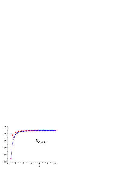
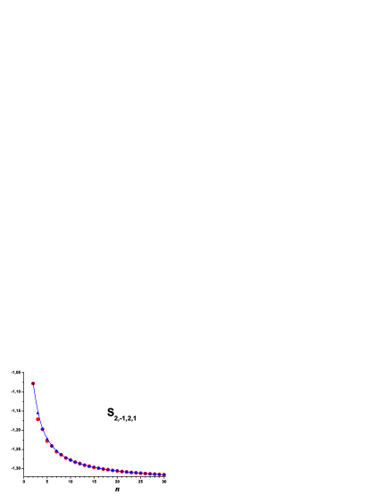
Figure 3: As in Fig. 2 but for the sums $S_{-3,-1,1,1}(n)$ and $S_{2,-1,2,1}(n)$.

$$S_{-a,-b,...}(n)~{}=~{}\sum_{m=1}^{n}\frac{(-1)^{m}}{m^{a}}S_{-b,...}(m).$$ (A5)

To demonstrate the nonsmooth behavior of such type of the nested sums, we show the sum $S_{-3,-1,1,1}(n)$ in Fig. 3.

Using the Eq. (22), we can express the function $(-1)^{m}S_{-b,...}(m)$ in the r.h.s. of (A5) as a combination of the smooth function $\overline{S}_{-b,...}^{+}(m)$ and some simpler functions and, thus, we have

$$S_{-a,-b,...}(n) = \sum_{m=1}^{n}\frac{1}{m^{a}}\biggl{[}\overline{S}^{+}_{-b,...}(m)-(1-(-1)^{m})Z_{-b,...}\biggr{]}$$ (A6)

$$= \sum_{m=1}^{n}\frac{1}{m^{a}}\overline{S}^{+}_{-b,...}(m)+Z_{-b,...}\biggl{[}S_{-a}(n)-S_{a}(n)\biggr{]}.$$

One can see that only one function $S_{-a}(n)$ is nonsmooth one in the r.h.s. of (A6).

Then, we have for the analytical continuation of $S_{-a,-b,...}(n)$:

$$\overline{S}^{+}_{-a,-b,...}(n)~{}=~{}\sum_{m=1}^{n}\frac{1}{m^{a}}\overline{S}^{+}_{-b,...}(m)+Z_{-b,...}\biggl{[}\overline{S}^{+}_{-a}(n)-S_{a}(n)\biggr{]}.$$ (A7)

Taking the difference of Eqs. (A6) and (A7), we obtain

$$\overline{S}^{+}_{-a,-b,...}(n)-S_{-a,-b,...}(n) = Z_{-b,...}\biggl{[}\overline{S}^{+}_{-a}(n)-S_{-a}(n)\biggr{]}$$ (A8)

$$= (1-(-1)^{n})Z_{-b,...}\biggl{[}Z_{-a}-S_{-a}(n)\biggr{]}.$$

From definitions (1) and (2) (by analogy with Eqs. (12) and (27)) we have that

$$Z_{-a,-b}~{}=~{}\zeta(-a,-b)+\zeta(a+b),$$

$$Z_{-a,-b,c}~{}=~{}\zeta(-a,-b,c)+\zeta(a+b,c)+\zeta(-a,-(b+c))+\zeta(a+b+c),$$

$$Z_{-a,-b,c,d}~{}=~{}\zeta(-a,-b,c,d)+\zeta(a+b,c,d)+\zeta(-a,-(b+c),d)+\zeta(-a,-b,c+d)$$

$$\vspace{1cm}+\zeta(a+b+c,d)+\zeta(a+b,c+d)+\zeta(-a,-(b+c+d))+\zeta(a+b+c+d).$$ (A9)

The results for $S_{-3,-1,1,1}(n)$ are presented in Fig. 3, where the function $\overline{S}^{+}_{-3,-1,1,1}(n)$ demonstrates its smooth $n$ behavior.

3. Now consider the sum $S_{a,-b,...}(n)$, which coincide in the case of two subscripts with one studied already in the subsection 1.

To demonstrate the nonsmooth behavior of such type of the nested sums, we show the sum $S_{2,-1,2,1}(n)$ in Fig. 3.

By analogy with the previous subsection we can represent the function $S_{a,-b,...}(n)$ to the form

$$S_{a,-b,...}(n)~{}=~{}\sum_{m=1}^{n}\frac{1}{m^{a}}S_{-b,...}(m)~{}=~{}\sum_{m=1}^{n}\frac{(-1)^{m}}{m^{a}}(-1)^{m}S_{-b,...}(m).$$ (A10)

Using the Eq. (22) we can express the function $(-1)^{m}S_{-b,...}(m)$ as a combination of the smooth function $\overline{S}_{-b,...}^{+}(m)$ and some simpler functions

$$S_{a,-b,...}(n) = \sum_{m=1}^{n}\frac{(-1)^{m}}{m^{a}}\biggl{[}\overline{S}^{+}_{-b,...}(m)-(1-(-1)^{m})Z_{-b,...}\biggr{]}$$ (A11)

$$= \sum_{m=1}^{n}\frac{(-1)^{m}}{m^{a}}\overline{S}^{+}_{-b,...}(m)+Z_{-b,...}\biggl{[}S_{a}(n)-S_{-a}(n)\biggr{]}.$$

One can see that the function $S_{-a}(n)$ is nonsmooth. Moreover, the first term in the r.h.s. contains the smooth function $\overline{S}_{-b,...}^{+}(m)$ and, thus, it can be continuated to odd $n$ values by analogy with the Eq. (22).

Then, we have the analytical continuation of $S_{a,-b,...}(n)$ as

$$\overline{S}^{+}_{a,-b,...}(n) = (-1)^{n}\sum_{m=1}^{n}\frac{(-1)^{m}}{m^{a}}\overline{S}^{+}_{-b,...}(m)+(1-(-1)^{n})\sum_{m=1}^{\infty}\frac{(-1)^{m}}{m^{a}}\overline{S}^{+}_{-b,...}(m)$$ (A12)

$$+ Z_{-b,...}\biggl{[}S_{a}(n)-\overline{S}^{+}_{-a}(n)\biggr{]}.$$

Using Eqs. (18) and (22) to represent the functions $\overline{S}^{+}_{-a}(n)$ and $\overline{S}^{+}_{-b,...}(m)$ as combinations of $S_{-a}(n)$, $Z_{-a}$, $S_{-b,...}(m)$ and $Z_{-b,...}$, we have the final result

$$\overline{S}^{+}_{a,-b,...}(n)~{}=~{}(-1)^{n}S_{a,-b,...}(n)+(1-(-1)^{n})\biggl{[}Z_{a,-b,...}-Z_{-b,...}\Bigl{(}Z_{a}-S_{a}(n)\Bigr{)}\biggr{]}.$$ (A13)

From definitions (1) and (2) we have that

$$Z_{a,-b}~{}=~{}\zeta(a,-b)+\zeta(-(a+b)),$$

$$Z_{a,-b,c}~{}=~{}\zeta(a,-b,c)+\zeta(-(a+b),c)+\zeta(a,-(b+c))+\zeta(-(a+b+c)),$$

$$Z_{a,-b,c,d}~{}=~{}\zeta(a,-b,c,d)+\zeta(-(a+b),c,d)+\zeta(a,-(b+c),d)+\zeta(-(a+b+c),d)$$

$$\vspace{1cm}+\zeta(a,-b,c+d)+\zeta(-(a+b),c+d)+\zeta(a,-(b+c+d))+\zeta(-(a+b+c+d)).$$ (A14)

One can see that the results coincide with the Eq. (A4) in the case of two subscripts.

The results for $S_{2,-1,2,1}(n)$ are presented in Fig. 3, where the function $\overline{S}^{+}_{2,-1,2,1}(n)$ demonstrates its smooth $n$ behavior.

4. Consider the sum $S_{a,-b,-c,...}(n)$. By analogy with the subsection 2 we have

$$S_{a,-b,-c,...}(n)~{}=~{}\sum_{m=1}^{n}\frac{1}{m^{a}}S_{-b,-c,...}(m).$$ (A15)

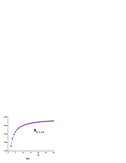
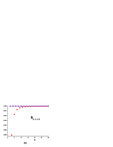
Figure 4: The circles are represented the sum $S_{2,-1,-1,3}(n)$ and the difference $\overline{S}_{2,-1,-1,3}^{+}(n)-S_{2,-1,-1,3}(n)$ (in the parts (a) and (b), respectively).

Using the Eq. (A8), we can express the function $S_{-b,-c,...}(m)$ as a combination of the smooth function $\overline{S}_{-b,-c,...}^{+}(m)$ and some simpler functions:

$$S_{a,-b,-c,...}(n) = \sum_{m=1}^{n}\frac{1}{m^{a}}\biggl{[}\overline{S}^{+}_{-b,-c,...}(m)-(1-(-1)^{m})Z_{-c,...}\Bigl{[}Z_{-b}-S_{-b}(m)\Bigr{]}\biggr{]}$$ (A16)

$$~{}=~{}\sum_{m=1}^{n}\frac{1}{m^{a}}\overline{S}^{+}_{-b,-c,...}(m)+Z_{-c,...}\biggl{[}Z_{-b}\Bigl{(}S_{-a}(n)-S_{a}(n)\Bigr{)}-S_{-a,-b}(n)+S_{a,-b}(n)\biggr{]}.$$

One can see that only the functions $S_{-a}(n)$, $S_{-a,-b}(n)$ and $S_{a,-b}(n)$ are nonsmooth one.

Then, we have for the analytical continuation of $S_{a,-b,-c,...}(n)$:

$$\overline{S}^{+}_{a,-b,-c,...}(n) = \sum_{m=1}^{n}\frac{1}{m^{a}}\overline{S}^{+}_{-b,-c...}(m)+Z_{-c,...}\biggl{[}Z_{-b}\Bigl{(}\overline{S}_{-a}^{+}(n)-S_{a}(n)\Bigr{)}$$ (A17)

$$- \overline{S}^{+}_{-a,-b}(n)+\overline{S}^{+}_{a,-b}(n)\biggr{]}.$$

Taking the difference of Eqs. (A16) and (A17), we obtain

$$\overline{S}^{+}_{a,-b,-c,...}(n) - S_{a,-b,-c,...}(n)~{}=~{}Z_{-c,...}\biggl{[}Z_{-b}\Bigl{(}\overline{S}_{-a}^{+}(n)-S_{-a}(n)\bigr{)}$$ (A18)

$$- \Bigl{(}\overline{S}^{+}_{-a,-b}(n)-S_{-a,-b}(n)\Bigr{)}+\Bigl{(}\overline{S}^{+}_{a,-b}(n)-S_{a,-b}(n)\Bigr{)}\biggr{]}$$

$$= (1-(-1)^{n})Z_{-c,...}\biggl{[}Z_{a,-b}-S_{a,-b}(n)-Z_{-b}\Bigr{(}Z_{a}-S_{a}(n)\Bigr{)}\biggr{]}.$$

From definitions (1) and (2) we have that

$$Z_{a,-b,-c}~{}=~{}\zeta(a,-b,-c)+\zeta(-(a+b),-c)+\zeta(a,b+c)+\zeta(a+b+c),$$

$$Z_{a,-b,-c,d}~{}=~{}\zeta(a,-b,-c,d)+\zeta(-(a+b),-c,d)+\zeta(a,b+c,d)+\zeta(a,-b,-(c+d))$$

$$\vspace{1cm}+\zeta(a+b+c,d)+\zeta(-(a+b),-(c+d))+\zeta(a,b+c+d)+\zeta(a+b+c+d).$$ (A19)

As an example, we show the sum $S_{2,-1,-1,3}(n)$ in Fig. 4(a). For the nested sums, where the first index $a$ is positive, the difference between two function, which are generated at even and odd $n$ values, are not so strong (see also, for example, the nested sums $S_{-3,-1,1,1}(n)$ and $S_{2,-1,-1,3}(n)$ in Fig. 3).

To demonstrate the effect of the analytic continuation, we show in Fig. 4(b) (by circles) the difference between $S_{2,-1,-1,3}(n)$ and the function, which is approximated from even $n$ values to integer ones. We see the effect of the difference at the odd $n$ values (essentially at $n=3,5,7$). After the analytic continuation, the difference become to be zero, that it is shown by triangles in Fig. 4(b).

5. Consider the sum $S_{-a,b,-c,...}(n)$. To demonstrate the nonsmooth behavior of such type of the nested sums, we show the sum $S_{-2,1,-2,1,1}(n)$ in Fig.  5.

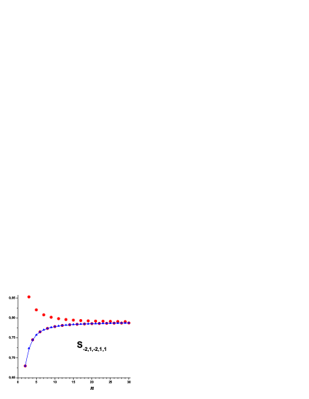
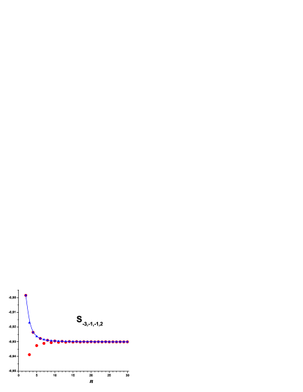
Figure 5: As in Fig. 2 but for the sum $S_{-2,1,-2,1,1}(n)$ and $S_{-3,-1,-1,2}(n)$.

By analogy with the subsections 2 and 4 we have

$$S_{-a,b,-c,...}(n)~{}=~{}\sum_{m=1}^{n}\frac{(-1)^{m}}{m^{a}}S_{b,-c,...}(m).$$ (A20)

Using the Eq. (A13), we can express the function $(-1)^{m}S_{b,-c,...}(m)$ as a combination of the smooth function $\overline{S}_{b,-c,...}^{+}(m)$ and some simpler functions:

$$S_{-a,b,-c,...}(n) = \sum_{m=1}^{n}\frac{1}{m^{a}}\biggl{[}\overline{S}^{+}_{b,-c,...}(m)-(1-(-1)^{m})\biggl{(}Z_{b,-c,...}-Z_{-c,...}\Bigl{[}Z_{b}-S_{b}(m)\Bigr{]}\biggr{)}\biggr{]}$$ (A21)

$$= \sum_{m=1}^{n}\frac{1}{m^{a}}\overline{S}^{+}_{b,-c,...}(m)+\biggl{(}Z_{b,-c,...}-Z_{b}Z_{-c,...}\biggr{)}\Bigl{[}S_{-a}(n)-S_{a}(n)\Bigr{]}$$

$$+ Z_{-c,...}\biggr{[}S_{-a,b}(n)-S_{a,b}(n)\biggr{]}.$$

One can see that only the functions $S_{-a}(n)$ and $S_{-a,b}(n)$ are nonsmooth one.

Then, we have for the analytical continuation of $S_{-a,b,-c,...}(n)$:

$$\overline{S}^{+}_{-a,b,-c,...}(n) = \sum_{m=1}^{n}\frac{1}{m^{a}}\overline{S}^{+}_{b,-c...}(m)+\biggl{(}Z_{b,-c,...}-Z_{b}Z_{-c,...}\biggr{)}\Bigl{[}\overline{S}^{+}_{-a}(n)-S_{a}(n)\Bigr{]}$$ (A22)

$$+ Z_{-c,...}\biggr{[}\overline{S}^{+}_{-a,b}(n)-S_{a,b}(n)\biggr{]}.$$

Taking the difference of Eqs. (A21) and (A22), we obtain

$$\overline{S}^{+}_{-a,b,-c,...}(n) - S_{-a,b,-c,...}(n)~{}=~{}\biggl{(}Z_{b,-c,...}-Z_{b}Z_{-c,...}\biggr{)}\Bigl{[}\overline{S}^{+}_{-a}(n)-S_{-a}(n)\Bigr{]}$$ (A23)

$$+ Z_{-c,...}\biggr{[}\overline{S}^{+}_{-a,b}(n)-S_{-a,b}(n)\biggr{]}$$

$$~{}=~{}(1-(-1)^{n})\Biggl{(}\biggl{[}Z_{b,-c,...}-Z_{b}Z_{-c,...}\biggr{]}\Bigl{[}Z_{-a}-S_{-a}(n)\Bigr{]}+Z_{-c,...}\biggr{[}Z_{-a,b}-S_{-a,b}(n)\biggr{]}\Biggr{)}.$$

From definitions (1) and (2) we have that

$$\ \ Z_{-a,b,-c}=\zeta(-a,b,-c)+\zeta(-(a+b),-c)+\zeta(-a,-(b+c))+\zeta(a+b+c),$$

$$\ \ Z_{-a,b,-c,d}=\zeta(-a,b,-c,d)+\zeta(-(a+b),-c,d)+\zeta(-a,-(b+c),d)+\zeta(-a,b,-(c+d))$$

$$\ \ \vspace{1cm}+\zeta(a+b+c,d)+\zeta(-(a+b),-(c+d))+\zeta(-a,-(b+c+d))+\zeta(a+b+c+d).$$ (A24)

The results for $S_{-2,1,-2,1,1}(n)$ are presented in Fig. 5, where the function $\overline{S}^{+}_{-2,1,-2,1,1}(n)$ demonstrates its smooth $n$ behavior.

6. Consider the sum $S_{a,b,-c,...}(n)$

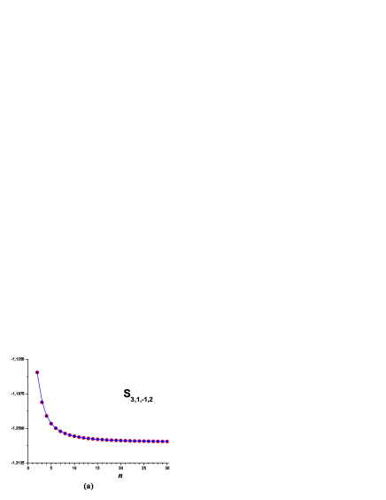
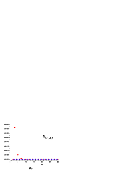
Figure 6: As in Fig. 4 but for the sum $S_{3,1,-1,2}(n)$.

By analogy with the subsections 3 and 5 we have

$$S_{a,b,-c,...}(n)~{}=~{}\sum_{m=1}^{n}\frac{1}{m^{a}}S_{b,-c,...}(m)~{}=~{}\sum_{m=1}^{n}\frac{(-1)^{m}}{m^{a}}(-1)^{m}S_{b,-c,...}(m).$$ (A25)

Using the Eq. (A13), we can express the function $(-1)^{m}S_{b,-c,...}(m)$ as a combination of the smooth function $\overline{S}_{b,-c,...}^{+}(m)$ and some simpler functions:

$$S_{a,b,-c,...}(n) = \sum_{m=1}^{n}\frac{(-1)^{m}}{m^{a}}\biggl{[}\overline{S}^{+}_{b,-c,...}(m)-(1-(-1)^{m})\biggl{(}Z_{b,-c,...}-Z_{-c,...}\Bigl{[}Z_{b}-S_{b}(m)\Bigr{]}\biggr{)}\biggr{]}$$ (A26)

$$= \sum_{m=1}^{n}\frac{(-1)^{m}}{m^{a}}\overline{S}^{+}_{b,-c,...}(m)+\biggl{(}Z_{b,-c,...}-Z_{b}Z_{-c,...}\biggr{)}\Bigl{[}S_{a}(n)-S_{-a}(n)\Bigr{]}$$

$$+ Z_{-c,...}\biggr{[}S_{a,b}(n)-S_{-a,b}(n)\biggr{]}.$$

One can see that the functions $S_{-a}(n)$ and $S_{-a,b}(n)$ are nonsmooth one. Moreover, the first term in the r.h.s. contains the smooth function $\overline{S}_{b,-c,...}^{+}(m)$ and, thus, can be continuated by analogy with the Eq. (A13).

Then, we have for the analytical continuation of $S_{a,b,-c,...}(n)$:

$$\overline{S}^{+}_{a,b,-c,...}(n) = (-1)^{n}\sum_{m=1}^{n}\frac{(-1)^{m}}{m^{a}}\overline{S}^{+}_{b,-c...}(m)+(1-(-1)^{n})\sum_{m=1}^{\infty}\frac{(-1)^{m}}{m^{a}}\overline{S}^{+}_{b,-c...}(m)$$ (A27)

$$-\biggl{(}Z_{b,-c,...}-Z_{b}Z_{-c,...}\biggr{)}\Bigl{[}\overline{S}^{+}_{-a}(n)-S_{a}(n)\Bigr{]}-Z_{-c,...}\biggr{[}\overline{S}^{+}_{-a,b}(n)-S_{a,b}(n)\biggr{]}.$$

Using Eqs. (18), (22) and (A13) to represent the functions $\overline{S}^{+}_{-a}(n)$, $\overline{S}^{+}_{-a,b,...}(n)$ and $\overline{S}^{+}_{b,-c,...}(m)$ as combinations of $S_{-a}(n)$, $Z_{-a}$, $S_{-a,b,...}(n)$, $Z_{-a,b,...}$, $S_{b,-c,...}(m)$ and $Z_{b,-c,...}$.

After some algebra we have the final result

$$\overline{S}^{+}_{a,b,-c,...}(n) = (-1)^{n}S_{a,b,-c,...}(n)~{}+~{}(1-(-1)^{n})\Biggl{(}Z_{a,b,-c,...}$$ (A28)

$$- \biggl{[}Z_{b,-c,...}-Z_{b}Z_{-c,...}\biggr{]}\Bigl{[}Z_{a}-S_{a}(n)\Bigr{]}-Z_{-c,...}\biggr{[}Z_{a,b}-S_{a,b}(n)\biggr{]}\Biggr{)}.$$

From definitions (1) and (2) we have that

$$Z_{a,b,-c}~{}=~{}\zeta(a,b,-c)+\zeta(a+b,-c)+\zeta(a,-(b+c))+\zeta(-(a+b+c)),$$

$$Z_{a,b,-c,d}~{}=~{}\zeta(a,b,-c,d)+\zeta(a+b,-c,d)+\zeta(a,-(b+c),d)+\zeta(-(a+b+c),d)$$

$$\vspace{1cm}+\zeta(a,b,-(c+d))+\zeta(a+b,-(c+d))+\zeta(a,-(b+c+d))+\zeta(-(a+b+c+d)).$$ (A29)

As an example, we show the sum $S_{3,1,-1,2}(n)$ in Fig. 6(a). By analogy with the subsection 4, to demonstrate the effect of the analytic continuation, we show in Fig. 6(b) (by circles) the difference between $S_{3,1,-1,2}(n)$ and the function, which is approximated from even $n$ values to integer ones. We see the effect of the difference at the odd $n$ values (essentially at $n=3,5,7$). After the analytic continuation, the difference become to be zero, that it is shown by triangles in Fig. 6(b).

7. As a last one we consider the sum $S_{-a,-b,-c,...}(n)$. To demonstrate the nonsmooth behavior of such type of the nested sums, we show the sum $S_{-3,1,-1,2}(n)$ in Fig.  5.

By analogy with the subsections 2 and 4 we have

$$S_{-a,-b,-c,...}(n)~{}=~{}\sum_{m=1}^{n}\frac{(-1)^{m}}{m^{a}}S_{-b,-c,...}(m).$$ (A30)

Using the Eq. (A8), we can express the function $S_{-b,-c,...}(m)$ as a combination of the smooth function $\overline{S}_{-b,-c,...}^{+}(m)$ and some simpler functions:

$$S_{-a,-b,-c,...}(n) = \sum_{m=1}^{n}\frac{(-1)^{m}}{m^{a}}\biggl{[}\overline{S}^{+}_{-b,-c,...}(m)-(1-(-1)^{m})Z_{-c,...}\Bigl{[}Z_{-b}-S_{-b}(m)\Bigr{]}\biggr{]}$$ (A31)

$$~{}=~{}\sum_{m=1}^{n}\frac{(-1)^{m}}{m^{a}}\overline{S}^{+}_{-b,-c,...}(m)+Z_{-c,...}\biggl{[}Z_{-b}\Bigl{(}S_{a}(n)-S_{-a}(n)\Bigr{)}+S_{-a,-b}(n)-S_{a,-b}(n)\biggr{]}.$$

One can see that the functions $S_{-a}(n)$, $S_{-a,-b}(n)$ and $S_{a,-b}(n)$ are nonsmooth. Moreover, the first term in the r.h.s. contains the smooth function $\overline{S}_{-b,-c,...}^{+}(m)$ and, thus, can be continuated by analogy with the Eq. (A8).

Then, we have for the analytical continuation of $S_{a,-b,-c,...}(n)$:

$$\overline{S}^{+}_{-a,-b,-c,...}(n) = (-1)^{n}\sum_{m=1}^{n}\frac{(-1)^{m}}{m^{a}}\overline{S}^{+}_{-b,-c,...}(m)+(1-(-1)^{n})\sum_{m=1}^{\infty}\frac{(-1)^{m}}{m^{a}}\overline{S}^{+}_{-b,-c,...}(m)$$ (A32)

$$- Z_{-c,...}\biggl{[}Z_{-b}\Bigl{(}\overline{S}_{-a}^{+}(n)-S_{a}(n)\Bigr{)}-\overline{S}^{+}_{-a,-b}(n)+\overline{S}^{+}_{a,-b}(n)\biggr{]}.$$

Using Eqs. (18), (22) and (A8) to represent the functions $\overline{S}^{+}_{-a}(n)$, $\overline{S}^{+}_{a,-b}(n)$ and $\overline{S}^{+}_{-b,-c,...}(m)$ as combinations of $S_{-a}(n)$, $Z_{-a}$, $S_{-b,...}(m)$ and $Z_{-b,...}$, we have the final result

$$\overline{S}^{+}_{-a,-b,-c,...}(n)\ =\ (-1)^{n}S_{-a,-b,-c,...}(n)$$

$$\ -\ (1-(-1)^{n})Z_{-c,...}\biggl{[}Z_{-a,-b}-S_{-a,-b}(n)-Z_{-b}\Bigr{(}Z_{-a}-S_{-a}(n)\Bigr{)}\biggr{]}.$$ (A33)

From definitions (1) and (2) we have that

$$Z_{-a,-b,-c}~{}=~{}\zeta(-a,-b,-c)+\zeta(a+b,-c)+\zeta(a,b+c)+\zeta(-(a+b+c)),$$

$$Z_{-a,-b,-c,d}~{}=~{}\zeta(-a,-b,-c,d)+\zeta(a+b,-c,d)+\zeta(-a,b+c,d)+\zeta(-a,-b,-(c+d))$$

$$\vspace{1cm}\,+\,\zeta(-(a+b+c),d)\!+\!\zeta(a+b,-(c+d))\!+\!\zeta(-a,-b+c+d)\!+\!\zeta(-(a+b+c+d)).$$ (A34)

The results for $S_{-3,1,-1,2}(n)$ are presented in Fig. 5, where the function $\overline{S}^{+}_{-3,1,-1,2}(n)$ demonstrates its smooth $n$ behavior.

9 Appendix B

Here we derive the analytic continuation of the nested sums

$$S_{a,-b,c,...}(n),~{}S_{-a,-b,c,...}(n),~{}S_{a,-b,-c,...}(n),~{}S_{-a,b,-c,...}(n),~{}S_{a,b,-c,...}(n),~{}S_{-a,-b,-c,...}(n)$$

from the even $n$ values to the real and/or complex $n$ values (the final results are presented in Section 4). As it was in Appendix A we will use here the definition (A1).

1. Consider firstly the sum $S_{-a,-b,...}(n)$. Using Eq. (A7) we rewrite the first term at the r.h.s. as follows

$$\sum_{m=1}^{n}\frac{1}{m^{a}}\overline{S}_{-b,...}^{+}(m)~{}=~{}\biggl{[}\sum_{m=1}^{\infty}-\sum_{m=n+1}^{\infty}\biggr{]}\frac{1}{m^{a}}\overline{S}_{-b,...}^{+}(m).$$ (B1)

The first term at the r.h.s. of (B1) is equal to

$$\sum_{m=1}^{\infty}\frac{1}{m^{a}}\overline{S}_{-b,...}^{+}(m)~{}=~{}Z_{-a,-b,...}+Z_{-b,...}\Bigl{[}Z_{a}-Z_{-a}\Bigr{]}.$$ (B2)

The second term can be defined as

$$\sum_{m=n+1}^{\infty}\frac{1}{m^{a}}\overline{S}_{-b,...}^{+}(m)~{}=~{}\sum_{l=0}^{\infty}\frac{1}{(l+n+1)^{a}}\overline{S}_{-b,...}^{+}(l+n+1)~{}\equiv~{}\Psi_{a,-b,...}(n+1),$$ (B3)

where the function $\Psi_{a,-b,...}(n+1)$ is well defined for the real and/or complex $n$ values.

Taking together Eqs. (19), (A7) and (B1)-(B3), we obtain the following result

$$\overline{S}_{-a,-b,...}^{+}(n)~{}=~{}Z_{-a,-b,...}-\Psi_{a,-b,...}(n+1)+Z_{-b,...}\Bigl{[}\Psi_{a}(n+1)-\Psi_{-a}(n+1)\Bigr{]},$$ (B4)

i.e. now the function $\overline{S}_{-a,-b,...}^{+}(n)$ contains objects well defined for the real and/or complex $n$ values.

2. Consider now the sum $S_{a,-b,...}(n)$. By analogy with the previous subsection, we rewrite the first term at the r.h.s. of Eq. (A12) as follows

$$\sum_{m=1}^{n}\frac{(-1)^{m}}{m^{a}}\overline{S}_{-b,...}^{+}(m)~{}=~{}\sum_{m=1}^{\infty}\frac{(-1)^{m}}{m^{a}}\overline{S}_{-b,...}^{+}(m)-\sum_{l=0}^{\infty}\frac{(-1)^{n+l+1}}{(l+n+1)^{a}}\overline{S}_{-b,...}^{+}(l+n+1)$$

$$=~{}Z_{a,-b,...}+Z_{-b,...}\Bigl{[}Z_{-a}-Z_{a}\Bigr{]}-(-1)^{n}\,\Psi_{-a,-b,...}(n+1).$$ (B5)

Taking together Eqs. (19), (A12) and (B5), we obtain the following result

$$\overline{S}_{a,-b,...}^{+}(n)~{}=~{}Z_{a,-b,...}-\Psi_{-a,-b,...}(n+1)+Z_{-b,...}\Bigl{[}\Psi_{-a}(n+1)-\Psi_{a}(n+1)\Bigr{]},$$ (B6)

i.e. now the function $\overline{S}_{a,-b,...}^{+}(n)$ is well defined for the real and/or complex $n$ values.

3. Consider the sums $S_{a,-b,-c,...}(n)$, $S_{-a,b,-c,...}(n)$, $S_{a,b,-c,...}(n)$ and $S_{-a,-b,-c,...}(n)$. By analogy with the previous subsections, the first term at the r.h.s. of Eqs. (A17), (A22), (A27) and (A32) can be represented in the following form, respectively,

$$\sum_{m=1}^{n}\frac{1}{m^{a}}\overline{S}_{-b,-c,...}^{+}(m)~{}=~{}\sum_{m=1}^{\infty}\frac{1}{m^{a}}\overline{S}_{-b,-c,...}^{+}(m)-\sum_{l=0}^{\infty}\frac{1}{(l+n+1)^{a}}\overline{S}_{-b,-c...}^{+}(l+n+1)$$

$$\qquad=~{}Z_{a,-b,-c,...}+Z_{-c,...}\biggr{[}Z_{-b}\Bigl{(}Z_{a}-Z_{-a}\Bigr{)}-Z_{a,-b}+Z_{-a,-b}\biggr{]}-\Psi_{a,-b,-c...}(n+1),$$ (B7)

$$\sum_{m=1}^{n}\frac{1}{m^{a}}\overline{S}_{b,-c,...}^{+}(m)\ =\ \sum_{m=1}^{\infty}\frac{1}{m^{a}}\overline{S}_{b,-c,...}^{+}(m)-\sum_{l=0}^{\infty}\frac{1}{(l+n+1)^{a}}\overline{S}_{b,-c...}^{+}(l+n+1)$$

$$\qquad=\ Z_{-a,b,-c,...}+\Bigl{[}Z_{b,-c,...}-Z_{b}Z_{-c,...}\Bigr{]}\Bigl{(}Z_{a}-Z_{-a}\Bigr{)}+Z_{-c,...}\Bigl{(}Z_{a,b}-Z_{-a,b}\Bigr{)}$$

$$\qquad-\ \Psi_{a,b,-c...}(n+1),$$ (B8)

$$\sum_{m=1}^{n}\frac{(-1)^{m}}{m^{a}}\overline{S}_{b,-c...}^{+}(m)~{}=~{}\sum_{m=1}^{\infty}\frac{(-1)^{m}}{m^{a}}\overline{S}_{b,-c,...}^{+}(m)-\sum_{l=0}^{\infty}\frac{(-1)^{n+l+1}}{(l+n+1)^{a}}\overline{S}_{b,-c,...}^{+}(l+n+1)$$

$$\qquad=\ Z_{a,b,-c,...}+\Bigl{[}Z_{b,-c,...}-Z_{b}Z_{-c,...}\Bigr{]}\Bigl{(}Z_{-a}-Z_{a}\Bigr{)}+Z_{-c,...}\Bigl{(}Z_{-a,b}-Z_{a,b}\Bigr{)}$$

$$\qquad-\ \Psi_{-a,b,-c...}(n+1).$$ (B9)

$$\sum_{m=1}^{n}\frac{(-1)^{m}}{m^{a}}\overline{S}_{-b,-c,...}^{+}(m)~{}=~{}\sum_{m=1}^{\infty}\frac{(-1)^{m}}{m^{a}}\overline{S}_{-b,-c,...}^{+}(m)-\sum_{l=0}^{\infty}\frac{(-1)^{l+n+1}}{(l+n+1)^{a}}\overline{S}_{-b,-c...}^{+}(l+n+1)$$

$$\qquad=~{}Z_{-a,-b,-c,...}+Z_{-c,...}\biggr{[}Z_{-b}\Bigl{(}Z_{-a}-Z_{a}\Bigr{)}+Z_{a,-b}-Z_{-a,-b}\biggr{]}-\Psi_{-a,-b,-c...}(n+1),$$ (B10)

Taking together Eqs. (19), (A17), (A22), (A27), (A32) and (B7)-(B10), we obtain the following results

$$\ \ \overline{S}_{a,-b,-c,...}^{+}(n)=Z_{a,-b,-c,...}-\Psi_{a,-b,-c,...}(n+1)~{}+~{}Z_{-c,...}\biggl{[}\Psi_{a,-b}(n+1)-\Psi_{-a,-b}(n+1)$$

$$\qquad-Z_{-b}\Bigl{(}\Psi_{a}(n+1)-\Psi_{-a}(n+1)\Bigr{)}\biggr{]},$$ (B11)

$$\ \ \overline{S}_{-a,b,-c,...}^{+}(n)=Z_{-a,b,-c,...}-\Psi_{a,b,-c,...}(n+1)~{}+~{}\Bigl{[}Z_{b,-c,...}-Z_{b}Z_{-c,...}\Bigr{]}$$

$$\qquad\times\Bigl{(}\Psi_{a}(n+1)-\Psi_{-a}(n+1)\Bigr{)}~{}+~{}Z_{-c,...}\Bigl{(}\Psi_{a,b}(n+1)-\Psi_{-a,b}(n+1)\Bigr{)},$$ (B12)

$$\ \ \overline{S}_{a,b,-c,...}^{+}(n)=Z_{a,b,-c,...}-\Psi_{-a,b,-c,...}(n+1)~{}+~{}\Bigl{[}Z_{b,-c,...}-Z_{b}Z_{-c,...}\Bigr{]}$$

$$\qquad\times\Bigl{(}\Psi_{-a}(n+1)-\Psi_{a}(n+1)\Bigr{)}~{}+~{}Z_{-c,...}\Bigl{(}\Psi_{-a,b}(n+1)-\Psi_{a,b}(n+1)\Bigr{)},$$ (B13)

$$\ \ \overline{S}_{-a,-b,-c,...}^{+}(n)=Z_{-a,-b,-c,...}-\Psi_{-a,-b,-c,...}(n+1)~{}+~{}Z_{-c,...}\biggl{[}\Psi_{-a,-b}(n+1)-\Psi_{a,-b}(n+1)$$

$$\qquad+Z_{-b}\Bigl{(}\Psi_{a}(n+1)-\Psi_{-a}(n+1)\Bigr{)}\biggr{]},$$ (B14)

i.e. now the functions $\overline{S}_{a,-b,-c,...}^{+}(n)$, $\overline{S}_{-a,b,-c,...}^{+}(n)$, $\overline{S}_{a,b,-c,...}^{+}(n)$ and $\overline{S}_{-a,-b,-c,...}^{+}(n)$ are well defined for the real and/or complex $n$ values.

References

[1] D.J. Gross and F. Wilczek, Phys. Rev. D8 (1973) 3633.
[2] W.A. Bardeen, A.J. Buras, D. Duke and T. Muta,
Phys. Rev. D18 (1978) 3998.
[3]
E.G. Floratos, D.A. Ross and C.T. Sachrajda, Nucl. Phys. B129 (1977) 66;
[Erratum-ibid. B139 (1978) 545];
E.G. Floratos, D.A. Ross and C.T. Sachrajda, Nucl. Phys. B152 (1979) 493;
A. Gonzalez-Arroyo, C. Lopez and F.J. Yndurain, Nucl. Phys. B153 (1979) 161;
A. Gonzalez-Arroyo and C. Lopez, Nucl. Phys. B166 (1980) 429;
E.G. Floratos, C. Kounnas and R. Lacage, Nucl. Phys. B192 (1981) 417;
G. Curci, W. Furmanski and R. Petronzio, Nucl. Phys. B175 (1980) 27;
W. Furmanski and R. Petronzio, Phys. Lett. B97 (1980) 437;
R. Hamberg and W. L. van Neerven, Nucl. Phys. B379 (1992) 143;
R.K. Ellis and W. Vogelsang, hep-ph/9602356.
[4] S. Moch, J.A. M. Vermaseren and A. Vogt,
Nucl. Phys. B688 (2004) 101.
[5] A. Vogt, S. Moch and J.A. M. Vermaseren,
Nucl. Phys. B691 (2004) 129.
[6]
D.A. Ross and C.T. Sachrajda, Nucl. Phys. B149 (1979) 497.
[7] A.L. Kataev and G. Parente, Phys. Lett. B566 (2003) 120.
[8] D.J. Broadhurst, A.L. Kataev and C.J. Maxwell,
Phys. Lett. B590 (2004) 76;
talk given at 32nd International Conference on High-Energy Physics (ICHEP 04),
Beijing, China, 16-22 Aug 2004 (hep-ph/0410058);
A.L. Kataev, talk at Workshop on Hadron Structure and QCD: From Low to High
Energies (HSQCD 2004), St. Petersburg, Repino, Russia, 18-22 May 2004
(hep-ph/0412369).
[9]
F.J. Yndurain, Phys. Lett. B74 (1978) 68.
[10]
G. Parisi and N. Sourlas, Nucl. Phys. B151 (1979) 421;
I.S. Barker, C.B. Langensiepen and G. Shaw,
Nucl. Phys. B186 (1981) 61;
I.S. Barker, B.R. Martin and G. Shaw,
Z. Phys. C19 (1983) 147;
I.S. Barker and B.R. Martin,
Z. Phys. C24 (1984) 255.
[11]
V.G. Krivokhizhin,
S.P. Kurlovich, V.V. Sanadze, I.A. Savin, A.V. Sidorov and
N.B. Skachkov, Z. Phys. C36 (1987) 51:
V.G. Krivokhizhin, S.P. Kurlovich, R. Lednicky, S. Nemechek,
V.V. Sanadze, I.A. Savin, A.V. Sidorov and N.B. Skachkov, Z. Phys. C48 (1990) 347.
[12]
V.N. Gribov and L.N. Lipatov, Sov. J. Nucl. Phys. bf 15 (1972) 438;
V.N. Gribov and L.N. Lipatov, Sov. J. Nucl. Phys. bf 15 (1972) 675;
L.N. Lipatov, Sov. J. Nucl. Phys. 20 (1975) 94;
G. Altarelli and G. Parisi, Nucl. Phys. B126 (1977) 298;
Yu.L. Dokshitzer, Sov. Phys. JETP 46 (1977) 641.
[13]
B. Escobles, M.J. Herrero, C. Lopez and
F.J. Yndurain, Nucl. Phys. B242 (1984) 329;
D. I. Kazakov and A. V. Kotikov,
Yad. Fiz. 46 (1987) 1767.
[14]
J. Santiago and F.J. Yndurain, Nucl. Phys. B563 (1999) 45;
B611 (2001) 447.
[15]
V.I. Vovk, Z. Phys. C47 (1990) 57;
A.V. Kotikov, G. Parente and J. Sanchez Guillen, Z. Phys. C58 (1993) 465;
V.G. Krivokhijine and A.V. Kotikov, hep-ph/0108224.
[16]
G. Parente, A.V. Kotikov and V.G. Krivokhizhin,
Phys. Lett. B333 (1994) 190.
[17]
A.L. Kataev, A.V. Kotikov, G. Parente and A.V. Sidorov,
Phys. Lett. B388 (1996) 179;
Phys. Lett. B417 (1998) 374;
Nucl. Phys. Proc. Suppl. 64 (1998) 138;
A.L. Kataev, G. Parente and A.V. Sidorov,
Nucl. Phys. B573 (2000) 405.
[18] A.D. Martin, R.G. Roberts, W.J. Stirling and R.S. Thorne,
Phys. Lett. B531 (2002) 216;
M. Glueck, E. Reya and A. Vogt,
Eur. Phys. J. C5 (1998) 461;
M. Gluck, C. Pisano, E. Reya, preprint DO-TH-2004-13 (hep-ph/0412049);
CTEQ Collab., J. Pumplin et al., JHEP 0207 (2002) 012.
[19]
S.A. Larin, T. van Ritbergen and J.A.M. Vermaseren,
Nucl. Phys. B427 (1994) 41;
S.A. Larin, P. Nogueira, T. van Ritbergen and J.A.M. Vermaseren,
Nucl. Phys. B492 (1997) 338;
A. Retey and J.A.M. Vermaseren,
Nucl. Phys. B604 (2001) 281.
[20]
L.N. Lipatov, Sov. J. Nucl. Phys. 23 (1976) 338;
V.S. Fadin, E.A. Kuraev and L. N. Lipatov, Phys. Lett. B 60 (1975) 50;
E.A. Kuraev, L.N. Lipatov and V. S. Fadin, Sov. Phys. JETP 44 (1976) 443;
E.A. Kuraev, L.N. Lipatov and V. S. Fadin, Sov. Phys. JETP 45 (1977) 199;
I.I. Balitsky and L.N. Lipatov, Sov. J. Nucl. Phys. 28 (1978) 822;
I.I. Balitsky and L.N. Lipatov, JETP Lett. 30 (1979) 355.
[23] L.N. Lipatov, Perspectives in Hadronic Physics, in:
Proc. of the ICTP conf. (World Scientific, Singapore, 1997);
L.N. Lipatov, in: Proc. of the Int. Workshop on very
high multiplicity physics, Dubna, 2000, pp.159-176;
L.N. Lipatov, Nucl. Phys. Proc. Suppl. 99A (2001) 175.
[24]
A.V. Kotikov, L.N. Lipatov, A.I. Onishchenko and V.N. Velizhanin,
Phys. Lett. B595 (2004) 521.
[25]
A.V. Kotikov, L.N. Lipatov and V.N. Velizhanin,
Phys. Lett. B557 (2003) 114.
[26]
F. Martin, Phys. Rev. D19 (1979) 1382;
C. Lopez and F.I. Yndurain,
Nucl. Phys. B171 (1980) 231.
[27]
C. Lopez and F.I. Yndurain,
Nucl. Phys. B183 (1981) 157.
[32] M. Gluck, E. Reya and A. Vogt, Z. Phys. C53
(1992) 651;
J. Blumlein, Comput. Phys. Commun. 133 (2000) 76.
[33] W.A. Bardeen, A.J. Buras, D.W. Duke and T. Muta,
Phys. Rev. D18 (1978) 3998;
G. Altarelli, R.K. Ellis and G. Martinelli, Nucl. Phys. B157 (1979) 461.
[34] D.I. Kazakov and A.V. Kotikov,
Theor. Math. Phys. 73 (1987) 1264;
A.V. Kotikov,
Theor. Math. Phys. 78 (1989) 134;
in Proceeding of the
XVth International Workshop ”High Energy Physics and Quantum Field Theory”,
Tver, September 2000
(hep-ph/0102177).
[35]
S. Moch and J.A.M. Vermaseren, Nucl. Phys. B573 (2000) 853.
[36]
S. Moch, J.A.M. Vermaseren and A. Vogt, Nucl. Phys. B646 (2002) 181.
[37] J. Blumlein,
Comput. Phys. Commun. 159 (2004) 19.
[38]
K.G. Chetyrkin, A.L. Kataev and F.V. Tkachov,
Nucl. Phys. B174 (1980) 345;
A.V. Kotikov,
Phys. Lett. B375 (1996) 240.
[39]
A. Buras, Rev. Mod. Phys. 52 (1980) 199.
[40] G. Altarelli, Phys. Rept. 81 (1982) 1.
[41]
K.G. Chetyrkin, F.V. Tkachov and S.G. Gorishnii,
Phys. Lett. B119 (1982) 407.
[43]
S. Moch and J.A.M. Vermaseren,
Nucl. Phys. Proc. Suppl. 86 (2000) 78; 89 (2000) 131, 137;
A. Vogt, S. Moch and J.A.M. Vermaseren, Nucl. Phys. Proc.
Suppl. 135 (2004) 137; talk at 12th International Workshop on Deep
Inelastic Scattering (DIS 2004), Strbske Pleso, Slovakia, 14-18 Apr 2004
and at the 11th International Conference in Quantum Chromodynamics (QCD 04),
Montpellier, France, 5-9 Jul 2004 (hep-ph/0407321).
[44] J. Fleischer, A.V. Kotikov and O.L. Veretin,
Phys. Lett. B417 (1998) 163;
Nucl. Phys. B547 (1999) 343;
Acta Phys. Polon. B29 (1998) 2611.
[45]
J.M. Borwein and R. Girgensohn, Electron. J. Combinations 3 (1996)
R23 (Appendix by D.J. Broadhurst);
J.M. Borwein, D.M. Bradley and D.J. Broadhurst,
arXiv:hep-th/9611004;
J.M. Borwein, D.J. Broadhurst and J. Kamnitzer, Exper. Math. 10
(2001) 25.
[46] D.I. Kazakov and A.V. Kotikov,
Phys. Lett. B291 (1992) 171.
[47] S. Moch, J.A.M. Vermaseren and A. Vogt,
paper in preparation.
[48] F.J. Yndurain, Quantum Chromodymanics. Introduction
to the Theory of Quarks and Gluons., Springer-Verlag (1983) New York.
[49] S. Moch, J.A.M. Vermaseren and A. Vogt,
Phys. Lett. B606 (2005) 123.
[50]
A.V. Kotikov, JETP Lett. 59 (1994) 667.
A.V. Kotikov and G. Parente,
Phys. Lett. B379 (1996) 195.
[51] A.V. Kotikov and G. Parente,
Nucl. Phys. B549 (1999) 242;
J. Exp. Theor. Phys. 97 (2003) 859;
A.Yu. Illarionov, A.V. Kotikov and G. Parente, hep-ph/0402173.
[52]
A.V. Kotikov, JETP Lett. 59 (1994) 1; Phys. Lett. B338 (1994) 349.
[53]
A.V. Kotikov, J. Exp. Theor. Phys. 80 (1995) 979;
A.V. Kotikov and G. Parente, J. Exp. Theor. Phys. 85 (1997) 17;
Mod. Phys. Lett. A12 (1997) 963.