Abstract

We consider emission of a photon by an electron in the field of a strong laser wave. A probability of this process for circularly or linearly polarized laser photons and for arbitrary polarization of all other particles is calculated. We obtain the complete set of functions which describe such a probability in a compact invariant form. Besides, we discuss in some detail the polarization effects in the kinematics relevant to the problem of $e\to\gamma$ conversion at $\gamma\gamma$ and $\gamma e$ colliders.

1 Introduction

The analysis of polarization effects in the Compton scattering

$$e(p)+\gamma(k)\to e(p^{\prime})+\gamma(k^{\prime})$$ (1)

is now included in text-books (see, for example, [1], §87). Nevertheless, the complete results for the cross sections with both initial and final particles polarized has been obtained only recently (see [2, 3, 4] and the literature therein). One interesting application of the process (1) is the collision of an ultra-relativistic electron with a beam of polarized laser photons. In this case the Compton effect is the basic process for obtaining of high-energy photons for contemporary experiments in nuclear physics and for future $\gamma\gamma$ and $\gamma e$ colliders [5]. The importance of the particle polarization is clearly seen from the fact that in comparison with the unpolarized case the number of final photons with maximum energy is nearly doubled when the helicities of the initial electron and photon are opposite [3].

With the growth of the laser field intensity, an electron starts to interact coherently with $n$ laser photons,

$$e(q)+n\,\gamma_{L}(k)\to e(q^{\prime})+\gamma(k^{\prime})\,,$$ (2)

thus the Compton scattering becomes non-linear. Such a process with absorption of $n=1,\,2,\,3,\,4$ linearly polarized laser photons was observed in the recent experiment at SLAC [6]. The polarization properties of the process (2) are important for future $\gamma\gamma$ and $\gamma e$ colliders (see [7, 8] and the literature therein). The non-linear Compton scattering must be taken into account in simulations of the processes in a conversion region of these colliders. For comprehensive simulation, including processes of multiple electron scattering, one has to know not only the differential cross section of the non-linear Compton scattering with a given number of the absorbed laser photons $n$, but energy, angles and polarization of final photons and electrons as well. The method of calculation for such cross sections was developed by Nikishov and Ritus [9]. It is based on the exact solution of the Dirac equation in the field of the external electromagnetic plane wave. Some particular polarization properties of this process were considered in [9]–[14] and have already been included in the existing simulation codes [13, 15].

In the paper [16] we presented the complete description of the non-linear Compton scattering for the case of circularly or linearly polarized laser photons and arbitrary polarization of all other particles. Besides, we derived (i) the approximate formulae relevant for the problem of $e\to\gamma$ conversion; (ii) the polarization of the final photons and electrons averaged over their azimuthal angles; (iii) the limiting cases of the small and large energies of the final photons; (iv) some numerical results obtained for the range of parameters close to those in the existing TESLA project [17]. Here we present the short review of the results obtained in [16].

We use the system of units in which $c=1$, $\hbar=1$. In what follows, we will often consider the non-linear Compton scattering in the frame of reference in which a high-energy electron performs a head-on collision with laser photons, i.e. in which ${\bf p}\,\parallel\,(-{\bf k})$. We call this the “collider system”. (For the case of non-head-on collision of the initial particles see  [16].)

2 Kinematics

Let us consider the interaction of an electron with a monochromatic plane wave. The corresponding electric and magnetic fields are ${\bf E}$ and ${\bf B}$, a frequency is $\omega$, and let $F$ be the root-mean-squared field strength, $F^{2}=\langle{\bf B}^{2}\rangle=\langle{\bf E}^{2}\rangle$ and $n_{\rm L}$ be the density of photons in the laser wave. The parameter describing the intensity of the laser field (the parameter of non-linearity) is defined as

$$\xi^{2}=\left({eF\over m\omega}\right)^{2}={4\pi\alpha\over m^{2}\,\omega}\,n_{\rm L}\,,$$ (3)

where $e$ and $m$ are the electron charge and the mass.

From the classical point of view, the oscillated electron emits harmonics with frequencies $n\,\omega$, where $n=1,\;2,\;\dots$ Their intensities at small $\xi^{2}$ are proportional to $({\bf E}^{2})^{n}\propto\xi^{2n}$, the polarization properties of these harmonics depend on the polarizations of the laser wave and the initial electron. From the quantum point of view, this radiation can be described as the non-linear Compton scattering with absorption of $n$ laser photons. When describing such a scattering, one has to take into account that in a field of the laser wave the 4-momenta $p$ and $p^{\prime}$ of the free initial and final electrons are replaced by the 4-quasi-momenta $q$ and $q^{\prime}$,

$$q=p+\xi^{2}{m^{2}\over 2pk}\,k\,,\;\;q^{\prime}=p^{\prime}+\xi^{2}{m^{2}\over 2p^{\prime}k}\,k\,,\;\;q^{2}=(q^{\prime})^{2}=(1+\xi^{2})\,m^{2}\,.$$ (4)

As a result, we deal with the reaction (2) for which the conservation law reads

$$q+n\,k=q^{\prime}+k^{\prime}\,.$$ (5)

Since $qk=pk$, it is convenient to use the same invariant variables as for the linear Compton scattering (compare [3]):

$$x={2pk\over m^{2}}\approx{4E\omega\over m^{2}}\,,\;\;\;y\;={kk^{\prime}\over pk}\approx{\omega^{\prime}\over E}\leq y_{n}={nx\over 1+nx+\xi^{2}}\,.$$ (6)

The invariant description of the polarization properties of both the initial and the final photons can be performed in the standard way (see [1], §87). We define a pair of unit 4-vectors

$$e^{(1)} = {N\over\sqrt{-N^{2}}}\,,\;\;\;e^{(2)}={P\over\sqrt{-P^{2}}}\,,$$ (7)

$$N^{\mu} = \varepsilon^{\mu\alpha\beta\gamma}P_{\alpha}(k^{\prime}-n\,k)_{\beta}K_{\gamma}\,,\;\;P_{\alpha}=(q+q^{\prime})_{\alpha}-{(q+q^{\prime})K\over K^{2}}\,K_{\alpha}\,,\;\;\;K_{\alpha}=n\,k_{\alpha}+k^{\prime}_{\alpha}\,.$$

The 4-vectors $e^{(1)}$ and $e^{(2)}$ are orthogonal to each other and to the 4-vectors $k$ and $k^{\prime}$, therefore, they are fixed with respect to the scattering plane of the process.

Let $\xi_{j}$ be the Stokes parameters for the initial photon which are defined with respect to 4-vectors $e^{(1)}$ and $e^{(2)}$. As for the polarization of the final photon, it is necessary to distinguish the polarization $\xi_{j}^{(f)}$ of the final photon as resulting from the scattering process itself from the detected polarization $\xi^{\prime}_{j}$ which enters the effective cross section and which essentially represents the properties of the detector as selecting one or other polarization of the final photon (for detail see [1], §65). Both these Stokes parameters, $\xi_{j}^{(f)}$ and $\xi^{\prime}_{j}$, are also defined with respect to the 4-vectors $e^{(1)}$ and $e^{(2)}$.

Let $\zeta$ be the polarization vector of the initial electrons. As with the final photon, it is necessary to distinguish the polarization $\zeta$^(f) of the final electron as such from the polarization $\zeta$^′ that is selected by the detector. The vectors $\zeta$ and $\zeta$^′ enter the effective cross section. They also determine the electron-spin 4-vectors $a$ and $a^{\prime}$.

Now we have to define invariants which describe the polarization properties of the initial and the final electrons. For the linear Compton scattering, the relatively simple description was obtained in  [2] using invariants which have a simple meaning in the center-of-mass system. However, this frame of reference is not convenient for the description of the non-linear Compton scattering, since it has actually to vary with the change of the number of the absorbed laser photons $n$.

Since $ap=a^{\prime}p^{\prime}=0$, we can decompose the electron polarization 4-vectors over three convenient unit 4-vectors $e_{j}$ and $e_{j}^{\prime}$, $j=1,\,2,\,3$, projections on which determine polarization properties of the electrons. Our choice is based on the experience obtained in [4] and [14]:

$$e_{1} = e^{(1)}\,,\;\;\;e_{2}=-e^{(2)}-{\sqrt{-P^{2}}\over m^{2}x}k\,,\;\;\;\;\;\;\;\;\;e_{3}={1\over m}\left(p-{2\over x}k\right);$$ (8)

$$e^{\prime}_{1} = e^{(1)}\,,\;\;\;e^{\prime}_{2}=-e^{(2)}-{\sqrt{-P^{2}}\over m^{2}x(1-y)}k\,,\;\;e^{\prime}_{3}={1\over m}\left(p^{\prime}-{2\over x(1-y)}k\right).$$

These vectors satisfy the conditions

$$e_{i}e_{j}=-\delta_{ij}\;,\;\;\;e_{j}p=0\;;\;\;\;e^{\prime}_{i}e^{\prime}_{j}=-\delta_{ij}\;,\;\;\;e^{\prime}_{j}p^{\prime}=0\,.$$ (9)

It allows us to represent the 4-vectors $a$ and $a^{\prime}$ in the following covariant form: $a=\sum_{j=1}^{3}\zeta_{j}e_{j}$,
$a^{\prime}=\sum_{j=1}^{3}\zeta^{\prime}_{j}e^{\prime}_{j}$, where

$$\zeta_{j}=-ae_{j}\,,\;\;\;\zeta^{\prime}_{j}=-a^{\prime}e^{\prime}_{j}\,.$$ (10)

3 Cross section in the invariant form

The usual notion of the cross section is not applicable for the reaction (2) and usually its description is given in terms of the probability of the process per second $\dot{W}^{(n)}$. However, for the procedure of simulation in the conversion region as well as for the simple comparison with the linear case, it is useful to introduce the “effective cross section” given by the definition

$$d\sigma^{(n)}={d\dot{W}^{(n)}\over j}\,,\;\;j={(q\,k)\over q_{0}\,\omega}\,n_{\rm L}={m^{2}\,x\over 2q_{0}\omega}\,n_{\rm L}\,,$$ (11)

where $j$ is the flux density of colliding particles. Contrary to the usual cross section, this effective cross section does depend on the laser beam intensity, i.e. on the parameter $\xi^{2}$. The total effective cross section is defined as the sum over harmonics, corresponding to the reaction (2) with a given number $n$ of the absorbed laser photons:

$$d\sigma=\sum\limits_{n}d\sigma^{(n)}\,.$$ (12)

The effective differential cross section can be presented in the following invariant form:

$$d\sigma(\mbox{\boldmath$\zeta$},\,\mbox{\boldmath$\xi$},\,\mbox{\boldmath$\zeta$}^{\prime},\,\mbox{\boldmath$\xi$}^{\prime})={r_{e}^{2}\over 4x}\;\sum_{n}F^{(n)}\;d\Gamma_{n}\,,\;\;d\Gamma_{n}=\delta(q+n\,k-q^{\prime}-k^{\prime})\;{d^{3}k^{\prime}\over\omega^{\prime}}{d^{3}q^{\prime}\over q_{0}^{\prime}}\,,$$ (13)

where $r_{e}=\alpha/m$ is the classical electron radius, and

$$F^{(n)}=F_{0}^{(n)}+\sum^{3}_{j=1}\left(F_{j}^{(n)}\xi^{\prime}_{j}\;+\;G_{j}^{(n)}\zeta^{\prime}_{j}\right)+\sum^{3}_{i,j=1}H_{ij}^{(n)}\,\zeta^{\prime}_{i}\,\xi^{\prime}_{j}\,.$$ (14)

In the collider system

$$d\Gamma_{n}=dy\,d\varphi\,,$$ (15)

where $\varphi$ is the azimuthal angle of the final photon. The function $F_{0}^{(n)}$ describes the total cross section for a given harmonic $n$, summed over spin states of the final particles:

$$\sigma^{(n)}(\mbox{\boldmath$\zeta$},\,\mbox{\boldmath$\xi$})={r_{e}^{2}\over x}\;\int F_{0}^{(n)}\,d\Gamma_{n}\,.$$ (16)

The terms $F_{j}^{(n)}\xi^{\prime}_{j}$ and $G_{j}^{(n)}\zeta^{\prime}_{j}$ in (14) describe the polarization of the final photons and the final electrons, respectively. The last terms $H_{ij}^{(n)}\zeta^{\prime}_{i}\,\xi^{\prime}_{j}$ stand for the correlation of the final particles’ polarizations.

From (13), (14) one can deduce the polarization of the final photon $\xi_{j}^{(f)}$ and electron $\zeta^{(f)}_{j}$ resulting from the scattering process itself. According to the usual rules (see [1], §65), we obtain the following expression for the Stokes parameters of the final photon (summed over polarization states of the final electron):

$$\xi_{j}^{(f)}={F_{j}\over F_{0}}\,,\;\;F_{0}=\sum_{n}F_{0}^{(n)}\,,\;\;F_{j}=\sum_{n}F_{j}^{(n)}\,;\;\;j=1,\,2,\,3\,.$$ (17)

The polarization of the final electron (summed over polarization states of the final photon) is given by invariants

$$\zeta_{j}^{(f)}={G_{j}\over F_{0}}\,,\;\;G_{j}=\sum_{n}G_{j}^{(n)}\,.$$ (18)

In the similar way, the polarization properties for a given harmonic $n$ are described by

$$\xi_{j}^{(n)(f)}={F_{j}^{(n)}\over F_{0}^{(n)}}\,,\;\;\zeta_{j}^{(n)(f)}={G_{j}^{(n)}\over F_{0}^{(n)}}\,.$$ (19)

As an example, we present here the functions $F_{0,1,2,3}$ for the circularly polarized laser photons. In this case the electromagnetic laser field is described by the 4-potential

$$A_{\mu}(x)={m\over e}\,\xi\;\left[e_{\mu}^{(1)}\,\cos{(kx)}+P_{c}\,e_{\mu}^{(2)}\,\sin{(kx)}\right]\,,$$ (20)

where the unit vectors $e_{\mu}^{(1,2)}$ are given in (7) and $P_{c}$ is the degree of the circular polarization of the laser wave or the initial photon helicity. We have calculated the coefficients $F_{j}^{(n)},\,G_{j}^{(n)}$ and $H_{ij}^{(n)}$ using the standard technique presented in [1], §101. The necessary traces have been calculated using the package MATHEMATICA. In the considered case of the 100 % circularly polarized ($P_{c}=\pm 1$) laser beam, almost all dependence on the non-linearity parameter $\xi^{2}$ accumulates in three functions:

$$f_{n} \equiv f_{n}(z_{n})=J_{n-1}^{2}(z_{n})+J_{n+1}^{2}(z_{n})-2J_{n}^{2}(z_{n})\,,$$

$$g_{n} \equiv g_{n}(z_{n})=\frac{4n^{2}J_{n}^{2}(z_{n})}{z_{n}^{2}}\,,$$ (21)

$$h_{n} \equiv h_{n}(z_{n})=J_{n-1}^{2}(z_{n})-J_{n+1}^{2}(z_{n})\,,$$

where $J_{n}(z)$ is the Bessel function. The functions (21) depend on $x$, $y$ and $\xi^{2}$ via the single argument

$$z_{n}={\xi\over\sqrt{1+\xi^{2}}}\;n\,s_{n}\,,$$ (22)

where

$$s_{n}=2\sqrt{r_{n}(1-r_{n})},\;\;c_{n}=1-2r_{n}\,,\;\;r_{n}={y\,(1+\xi^{2})\over(1-y)\,nx}\,.$$ (23)

For the small value of this argument one has

$$f_{n}=g_{n}=h_{n}=\frac{(z_{n}/2)^{2(n-1)}}{[(n-1)!]^{2}}\;\;\mbox{ at}\;\;z_{n}\to 0\,,$$ (24)

in particular,

$$f_{1}=g_{1}=h_{1}=1\;\;\mbox{ at}\;\;z_{1}=0\,.$$ (25)

The results of our calculations are the following. The function $F_{0}^{(n)}$, related to the total cross section (16), reads

$$F_{0}^{(n)}=\left({1\over 1-y}+1-y\right)\,f_{n}-{s_{n}^{2}\over 1+\xi^{2}}\,g_{n}-\left[{ys_{n}\over\sqrt{1+\xi^{2}}}\,\zeta_{2}-{y(2-y)\over 1-y}\,c_{n}\,\zeta_{3}\right]\,h_{n}\,P_{c}\,.$$ (26)

The polarization of the final photons $\xi_{j}^{(f)}$ is given by Eq. (17) where

$$F_{1}^{(n)} = {y\over 1-y}{s_{n}\over\sqrt{1+\xi^{2}}}\,h_{n}P_{c}\,\zeta_{1}\,,$$ (27)

$$F_{2}^{(n)} = \left({1\over 1-y}+1-y\right)\,c_{n}h_{n}P_{c}-{ys_{n}c_{n}\over\sqrt{1+\xi^{2}}}\,g_{n}\,\zeta_{2}+y\left({2-y\over 1-y}\,f_{n}-{s^{2}_{n}\over 1+\xi^{2}}\,g_{n}\right)\zeta_{3}\,,$$

$$F_{3}^{(n)} = 2(f_{n}-g_{n})+s^{2}_{n}(1+\Delta)\,g_{n}-{y\over 1-y}{s_{n}\over\sqrt{1+\xi^{2}}}\,h_{n}P_{c}\,\zeta_{2}$$

and $\Delta=\xi^{2}/(1+\xi^{2})$. Note that our results for $F_{0}^{(n)}$ and $F_{2}^{(n)}$ coincide with that ones in the literature, whereas the results for $F_{1}^{(n)}$ and $F_{3}^{(n)}$ are new.

4 Examples and discussion

In this section we give some examples which illustrate the dependence of the differential cross sections and the polarizations on the final photon energy. We restrict ourselves to properties of the high-energy photon beam which are of most importance for the future $\gamma\gamma$ and $\gamma e$ colliders. It is expected (see, for example, the TESLA project [17]) that in the conversion region of these colliders, an electron with the energy $E=250$ GeV performs a head–on collisions with laser photons having the energy $\omega\approx 1$ eV per a single photon. The parameters used below are close to those in the TESLA project. In particular,

$$x\approx 4E\omega/m^{2}=4.8\,,$$

and the non-linearity parameter $\xi^{2}$ (3) is chosen either the same as in the TESLA project, $\xi^{2}=0.3$, or larger by one order of magnitude, $\xi^{2}=3$, just to illustrate the tendencies. In figures below we use notation

$$\sigma_{0}=\pi r_{e}^{2}\approx 2.5\cdot 10^{-25}\;\;\mbox{cm}^{2}\,.$$

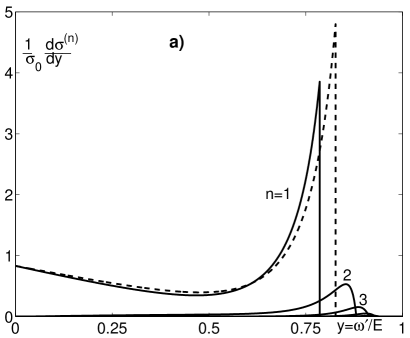
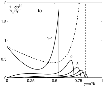
Figure 1: Energy spectra of final photons for different harmonics $n$ at $\zeta_{3}\,P_{c}=-1$ and: (a) $\xi^{2}=0.3$;   (b) $\xi^{2}=3$. The dashed curves correspond to $\xi^{2}=0$.

The case of the circularly polarized laser photons (Fig. 1).

The spectra of the few first harmonics are shown in Fig. 1 for the case of “a good polarization”, when helicities of the laser photon and the initial electron are opposite, $\zeta_{3}P_{c}=-1$. At a small intensity of the laser wave ($\xi^{2}=0.3$, Fig. 1a) the main contribution is given by photons of the first harmonic and the probability for generation of the higher harmonics is small. However, with the growth of the non-linearity parameter ($\xi^{2}=3$, Fig. 1b), the maximum energy for the first harmonic decreases and the peak of this harmonic at $y=y_{1}$ decreases as well. As for the higher harmonics, with the rise of $\xi^{2}$ (Fig. 1b) we see an increase of the yield of photons with energies higher than the maximum energy of the first harmonic. As a result, the total spectrum becomes considerable wider.

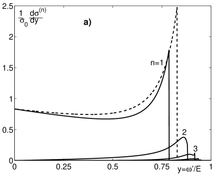
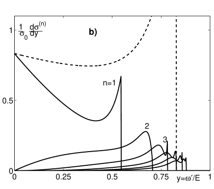
Figure 2: Energy spectra of final photons for different harmonics $n$ in the case of the linearly polarized laser photons and: (a) $\xi^{2}=0.3$;   (b) $\xi^{2}=3$. The dashed curves correspond to $\xi^{2}=0$.

The case of the linearly polarized laser photons (Figs. 2, 3, 4).

The spectra of the first few harmonics for this case are shown in Fig. 2. They differ considerably from those for the case of the circularly polarized laser photons shown in Fig. 1. First of all, in the considered case the spectra do not depend on the polarization of the initial electrons. The maximum of the spectrum for the first harmonic at $y=y_{1}$ now is about two times smaller than that on Fig. 1. Besides, the harmonics with $n>1$ do not vanish at $y=y_{n}$ contrary to such harmonics on Fig. 1.

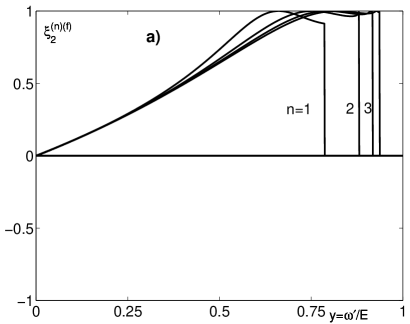
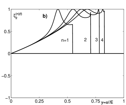
Figure 3: The mean helicity $\xi_{2}^{(n)(f)}$ of the final photons for different harmonics $n$ versus the final photon energy $\omega^{\prime}$ at $\zeta_{3}=1$ and: (a) $\xi^{2}=0.3$;   (b) $\xi^{2}=3$. The laser photons are linearly polarized. The scattering plane is parallel to the direction of the laser photon polarization.

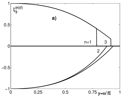
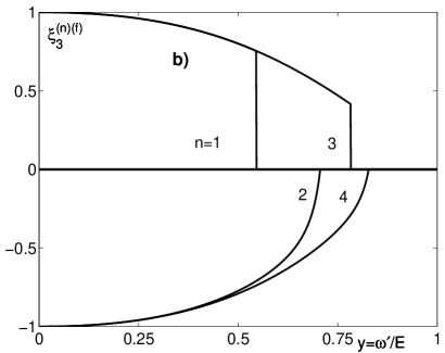
Figure 4: The Stokes parameters $\xi_{3}^{(n)(f)}$ of the final photons for different harmonics $n$ versus the final photon energy $\omega^{\prime}$ at $\zeta_{3}=1$ and: (a) $\xi^{2}=0.3$;   (b) $\xi^{2}=3$. The laser photons are linearly polarized. The scattering plane is perpendicular to the direction of the laser photon polarization. The Stokes parameter $\xi_{1}^{(n)(f)}=0$ in this case.

For the first few harmonics the mean helicities of the final photons, $\xi_{2}^{(n)(f)}$, are shown at $\zeta_{3}=1$ in Fig. 3a for $\xi^{2}=0.3$ and in Fig. 3b for $\xi^{2}=3$. We would like to direct attention to the surprising fact that each harmonic is almost 100% circularly polarized near the high-energy part of the spectrum. The curves on Fig. 3 are given for the azimuthal angle $\varphi=0$, for other values of $\varphi$ these curves would look a bit different, but not too much.

The degree of linear polarization of the final photons is not large in the high-energy part of the spectrum, but it becomes rather high in the middle and the low part of the spectrum; see Fig. 4. Certainly, the direction of this polarization depends on the azimuthal angle $\varphi$, as the result the linear polarization averaged over $\varphi$ is substantially smaller than one on Fig. 4. Nevertheless, the non-trivial effects, related to the high degree of linear polarization present at a certain $\varphi$, do exist. For example, it was shown [18] that for linear Compton scattering this feature leads to an important effect for the luminosity of $\gamma\gamma$ collisions.

References

- [1] V.B. Berestetskii, E.M. Lifshitz, L.P. Pitaevskii, Quantum electrodynamics, Nauka, Moscow, 1989
- [2] A.G. Grozin, Proceedings of Joint Inter. Workshop on High Energy Physics and Quantum Field Theory (Zvenigorod), ed. by B.B. Levtchenko, Moscow State Univ., Moscow, 1994, p. 60
- [3] I.F. Ginzburg, G.L. Kotkin, S.L. Panfil, V.G. Serbo, Yad. Fiz. 38 (1983) 1021; I.F. Ginzburg, G.L. Kotkin, S.L. Panfil, V.G. Serbo, V.I. Telnov, Nucl. Instr. Meth. 219 (1984) 5
- [4] G.L. Kotkin, S.I. Polityko, V.G. Serbo, Nucl. Instr. Meth. A 405 (1998). 30
- [5] I.F. Ginzburg, G.L. Kotkin, V.G. Serbo, V.I. Telnov, Nucl. Instr. Meth. 205 (1983) 47
- [6] C. Bula, K. McDonald et al., Phys. Rev. Lett. 76 (1996) 3116
- [7] I.F. Ginzburg, G.L. Kotkin, S.I. Polityko, Sov. Nucl. Phys. 40 (1984) 1495
- [8] M. Galynskii, E. Kuraev, M. Levchuk, V. Telnov, Nucl. Instrum. Meth. A 472 (2001) 267
- [9] A.I. Nikishov, V.I. Ritus, Zh. Eksp. Teor. Fiz. 46 (1964) 776; Trudy FIAN v. 111 (1979) (Proceedings of the Lebedev Institute, in Russian).
- [10] Ya.T. Grinchishin, M.P. Rekalo, Yad. Fiz. 40 (1984) 181
- [11] M.V. Galynskii, S.M. Sikach, Sov. Phys. JETP 74 (1992) 441 (in English)
- [12] Yu.S. Tsai, Phys. Rev. D 48 (1993) 96
- [13] K. Yokoya, CAIN2e Users Manual. The latest version is available from ftp://lcdev.kek.jp/pub/Yokoya/cain235/CainMan235.pdf.
- [14] E. Bol’shedvorsky, S. Polityko, A. Misaki, Prog. Theor. Phys. 104 (2000) 769
- [15] V.I. Telnov, Nucl. Instr. Meth. A355 (1995)
- [16] D.Yu. Ivanov, G.L. Kotkin, V.G. Serbo. Eur. Phys. J. C 36 (2004) 127
- [17] R. Brinkmann et al., Nucl. Instr. Meth. A 406 (1998) 13
- [18] S. Petrosyan, V. Serbo, V. Telnov, Nontrivial effects in linear polarization at photon colliders. ECFA Study “Physics and Detectors for a Linear Collider ” (November 13—16, 2003, Montpellier, France).