Two-flavor condensates in chiral dynamics: temperature and isospin density effects.

Abstract

Isospin density and thermal corrections for several condensates are discussed, at the one-loop level, in the frame of chiral dynamics with pionic degrees of freedom. The evolution of such objects give an additional insight into the condensed-pion phase transition, that occurs basically when $|\mu_{\mbox{\tiny I}}|>m_{\pi}$, being $|\mu_{\mbox{\tiny I}}|$ the isospin chemical potential. Calculations are done in both phases, showing a good agreement with lattice results for such condensates.

This paper is an extension of our previous analysis of pion dynamics, according to chiral perturbation theory, in the presence of isospin chemical potential and temperature. In the first article Loewe:2002tw we discussed the evolution of the masses and decay constants from the perspective of the first phase ($|\mu_{\mbox{\tiny I}}|<m_{\pi}$). In the second paper Loewe:2004mu , we proposed a scheme of calculation in the second phase for the pion masses ($|\mu_{\mbox{\tiny I}}|>m_{\pi}$). The method allowed us to explore the regions where the chemical potential is close to the phase transition point ($|\mu_{\mbox{\tiny I}}|\gtrsim m_{\pi}$) and also where $|\mu_{\mbox{\tiny I}}|\gg m_{\pi}$. The validity of this approach is restricted to values of $\mu_{\mbox{\tiny I}}$ less than the $\eta$ or $\rho$ masses.

Here we would like to address the thermal and density behavior of several condensates that can be buit in this frame, as well as the validity of the Gell-Mann–Oakes–Renner (GMOR) relation, completing in this way the discussion of the pion properties. We compare our results with those obtained through lattice measurements.

This analysis is relevant since some of these condensates are sharp signals for the occurrence of the phase transition, i.e., phenomenological order parameters. Natural scenarios where this dynamics can play a role are in the core of neutron stars (especially during the cooling period), possible asymmetries in the pion multiplicity in the central rapidity region at RHIC or ALICE, etc.

As in the previous articles, we introduce the chemical potential following Kogut:1999iv ; Kogut:2000ek . Even though, these articles deal with QCD with two colors rather than QCD with three colors, it is clear that both problems are intimately related. The introduction of in-medium processes via isospin chemical potential has been studied at zero temperature Son:2000xc ; Kogut:2001id in both phases ($|\mu_{\mbox{\tiny I}}|\lessgtr m_{\pi}$) at tree level.

Different approaches, such as Lattice QCD Kogut:2002tm ; Kogut:2002zg ; Kogut:2001if ; Kogut:2002cm , Ladder QCD Barducci:2003un and Nambu-Jona-Lasinio model based analysis Toublan:2003tt ; Frank:2003ve ; Barducci:2004tt ; Barducci:2004nc ; He:2005sp have confirmed the appearance of an interesting and non-trivial phase structure as function of temperature and chemical potentials, in particular isospin, chemical potential.

I Chiral Lagrangian

In the low-energy description where only pion degrees of freedom are relevant, the most general chiral invariant lagrangian at the second order, ${\cal O}(p^{2})$, according to an expansion in powers of the external momentum is given by

$${\cal L}_{2} = \frac{f^{2}}{4}Tr\left[(D_{\mu}U)^{\dagger}D^{\mu}U+U^{\dagger}\chi+\chi^{\dagger}U\right]$$ (1)

with

$$D_{\mu}U = \partial_{\mu}U-i[v_{\mu},U]-i\{a_{\mu},U\},$$ (2)

$$\chi = 2B(s+ip),$$ (3)

$$U = \bar{U}^{\mbox{\tiny$1/2$}}(e^{i\pi^{a}\tau^{a}/f})\bar{U}^{\mbox{\tiny$1/2$}},$$ (4)

$s=s^{0}(x)+s^{a}(x)\tau^{a}$, $p=p^{0}(x)+p^{a}(x)\tau^{a}$, $v_{\mu}=\frac{1}{2}v_{\mu}^{a}(x)\tau^{a}$ and $a_{\mu}=\frac{1}{2}a_{\mu}^{a}(x)\tau^{a}$ being the scalar, pseudo-scalar, vector and axial-vector external sources, respectively, where $\tau^{a}$ are the Pauli matrices. $\bar{U}$ is the vacuum expectation value of the field $U$. $M=diag(m_{u},m_{d})$ is the quark mass matrix and $B$ in the previous equation is an arbitrary constant which will be fixed when the mass is identified setting $(m_{u}+m_{d})B=m^{2}$, where $m$ denotes the bare (tree-level) pion mass. We will use $m_{\pi}$ to denote the pion masses after renormalization.

The most general ${\cal O}(p^{4})$ chiral lagrangian has the form

$${\cal L}_{4} = \textstyle{\frac{1}{4}}l_{1}\left(Tr\left[(D_{\mu}U)^{\dagger}D^{\mu}U\right]\right)^{2}$$ (5)

$$+\textstyle{\frac{1}{4}}l_{2}Tr\left[(D_{\mu}U)^{\dagger}D_{\nu}U\right]Tr\left[(D^{\mu}U)^{\dagger}D^{\nu}U\right]$$

$$+\textstyle{\frac{1}{16}}(l_{3}+l_{4})\left(Tr\left[\chi U^{\dagger}+U\chi^{\dagger}\right]\right)^{2}$$

$$+\textstyle{\frac{1}{8}}l_{4}Tr\left[(D_{\mu}U)^{\dagger}D^{\mu}U\right]Tr\left[\chi U^{\dagger}+U\chi^{\dagger}\right]$$

$$+l_{5}Tr\left[\big{(}L_{\mu\nu}U+UR_{\mu\nu}\big{)}\big{(}U^{\dagger}L^{\mu\nu}+R^{\mu\nu}U^{\dagger}\big{)}\right]$$

$$+l_{6}Tr\left[iL_{\mu\nu}D^{\mu}U(D^{\nu}U)^{\dagger}+iR_{\mu\nu}(D^{\mu}U)^{\dagger}D^{\nu}U\right]$$

$$-\textstyle{\frac{1}{16}}l_{7}\left(Tr\left[\chi U^{\dagger}-U\chi^{\dagger}\right]\right)^{2}+\textstyle{\frac{1}{4}}(\tilde{h}_{1}+\tilde{h}_{3})Tr[\chi^{\dagger}\chi]$$

$$-\textstyle{\frac{1}{8}}(\tilde{h}_{1}-\tilde{h}_{3})Tr\left[\left(\chi-Tr[\chi]\right)^{2}+\left(\chi^{\dagger}-Tr[\chi^{\dagger}]\right)^{2}\right]$$

$$-2\tilde{h}_{2}Tr\left[L_{\mu\nu}L^{\mu\nu}+R_{\mu\nu}R^{\mu\nu}\right],$$

The $l_{i}$ are the original Gasser and Leutwyler coupling constants Gasser:1983yg for an $SU(2)$ Lagrangian, and the $\tilde{h}_{i}$ constants are couplings to pure external fields, and their values are model dependent. They have to be determined experimentally and are also tabulated in several articles and books. This Lagrangian includes the chemical potentials in the covariant derivatives and in the expectation value of the $\bar{U}$ matrix. The constants $l_{i}$ include divergent corrections which allow to cancel the divergences from loops corrections constructed from the ${\cal L}_{2}$ Lagrangian

$$l_{i}(\Lambda)=\frac{\gamma_{i}}{32\pi^{2}}\left[\bar{l}_{i}-\lambda+\ln\left(\frac{m^{2}}{\Lambda^{2}}\right)\right]$$ (6)

with the $\overline{ms}$ pole

$$\lambda=\frac{2}{4-d}+\ln 4\pi+\Gamma^{\prime}(1)+1.$$ (7)

The $\tilde{h}_{i}$ constants do not include divergent terms.

For $|\mu_{\mbox{\tiny$I$}}|>m$ there is a symmetry breaking. The vacuum expectation value that minimizes the potential, calculated in Kogut:2001id , is

$$\bar{U} = \textstyle{\frac{m^{2}}{\mu_{\mbox{\tiny$I$}}^{2}}}+i[\tau_{1}\cos\phi+\tau_{2}\sin\phi]\sqrt{1-\textstyle{\frac{m^{4}}{\mu_{\mbox{\tiny$I$}}^{4}}}}$$ (8)

$$\equiv c+i\tilde{\tau}_{1}s,$$

where $c\equiv\frac{m^{2}}{\mu_{\mbox{\tiny$I$}}^{2}}$, $s\equiv\sqrt{1-\textstyle{\frac{m^{4}}{\mu_{\mbox{\tiny$I$}}^{4}}}}$. From now on, we will use a tilde to refer to any vector rotated in a $\phi$ angle

$$\tilde{v}_{1} = v_{1}\cos\phi+v_{2}\sin\phi$$

$$\tilde{v}_{2} = -v_{1}\sin\phi+v_{2}\cos\phi.$$ (9)

For our purposes it is enough to keep the ${\cal L}_{2,2}$ terms of the lagrangian to construct the Dolan-Jackiw propagators (DJp) which are the same as the ones we used in the previous articles, both in the first and in the second phase, respectively Loewe:2002tw ; Loewe:2004mu

In both phases the $\pi_{0}$ propagator will be the same, because it is always diagonal

$$D_{DJ}(p)_{00}=\frac{i}{p^{2}-m^{2}+i\epsilon}+2\pi n_{B}(|p_{0}|)\delta(p^{2}-m^{2})$$ (10)

In the first phase, where the charged pions do not mix, the thermal propagators are

$$D_{DJ}(p)_{+-}=\frac{i}{(p+\mu_{\mbox{\tiny I}}u)^{2}-m^{2}+i\epsilon}\\ +2\pi n_{B}(|p_{0}|)\delta\big{(}(p+\mu_{\mbox{\tiny I}}u)^{2}-m^{2}\big{)}$$ (11)

and $D_{DJ}(p)_{-+}=D_{DJ}(-p)_{+-}$.Those propagators refer to the fields $\pi_{+}$ and $\pi_{-}$. In the second phase, where the charged pion fields become mixed, the propagators have a non-trivial matrix structure (see Loewe:2004mu ). By scaling all the parameters and variables with $|\mu_{\mbox{\tiny I}}|$, it is possible to make an expansion in terms of an appropriate smallness parameter in powers of $s^{n}$ when $|\mu_{\mbox{\tiny I}}|\gtrsim m$ and $c^{n}$ when $|\mu_{\mbox{\tiny I}}|\gg m$, where $s$ and $c$ are defined in eq. (8). A similar expansion criteria was proposed earlier by Splittorff, Toublan and Verbaarschot Splittorff:2001fy ; Splittorff:2002xn . In this case we will use the lowest order term in the expansion and a negative isospin chemical potential $\mu_{\mbox{\tiny I}}=-|\mu_{\mbox{\tiny I}}|$, as in the case of neutron stars.

The DJp in the region where $|\mu_{\mbox{\tiny I}}|\gtrsim m$ are the same as in eq. (11) plus corrections of ${\cal O}(s^{2})$ referring to the fields $\tilde{\pi}_{+}$ and $\tilde{\pi}_{-}$. The other propagators $D_{DJ}(p)_{++}=D_{DJ}(p)_{--}$ are of order $s^{2}$.

In the case where $|\mu_{\mbox{\tiny I}}|\gg m$, it is better to work with the fields $\tilde{\pi}_{1}$ and $\tilde{\pi}_{2}$ instead of $\tilde{\pi}_{\pm}$. The DJp for the $\tilde{\pi}_{1}$ field is the same as the the $\pi_{0}$ propagator plus higher corrections: $D_{DJ}(p)_{11}=D_{DJ}(p)_{00}+\mu_{\mbox{\tiny I}}^{-2}{\cal O}(c^{2})$. For the $\tilde{\pi}_{2}$ propagator we have

$$D_{DJ}(p)_{22}=\frac{i}{p^{2}+i\epsilon}+2\pi n_{B}(|p_{0}|)\delta(p^{2})+\mu_{\mbox{\tiny I}}^{-2}{\cal O}(c^{2}),$$ (12)

The last propagator we will introduce is the mixed $\tilde{\pi}_{1}\tilde{\pi}_{2}$ propagator, which will be used in the loop calculation for the axial-charge density condensate

$$D_{DJ}(p)_{12} = -2ic\frac{p_{0}}{|\mu_{\mbox{\tiny I}}|}\bigg{\{}\frac{i}{p^{2}-\mu_{\mbox{\tiny I}}^{2}+i\epsilon}-\frac{i}{p^{2}+i\epsilon}$$ (13)

$$+2\pi n_{B}(|p_{0}|)\big{[}\delta(p^{2}-\mu_{\mbox{\tiny I}}^{2})-\delta(p^{2})\big{]}\bigg{\}}$$

$$+\mu_{\mbox{\tiny I}}^{-2}{\cal O}(c^{3}).$$

As in the case of the $\pi_{\pm}$ propagators, which are anti-diagonal in the propagator matrix, we have $D_{DJ}(p)_{21}=D_{DJ}(-p)_{12}$. The other possible propagators are zero in both phases: $D_{DJ}(p)_{3,a\neq 3}\equiv 0$

II Condensates

The different condensates can be constructed taking appropriate functional derivatives with respect to the external sources in the extended chiral lagrangian. In this way we will consider the following currents

$$V_{\mu}^{a}=\frac{\delta S}{\delta v_{\mu}^{a}} ={\textstyle{\frac{1}{2}}}\bar{q}\gamma_{\mu}\tau^{a}q, A_{\mu}^{a}=\frac{\delta S_{\chi}}{\delta a_{\mu}^{a}} ={\textstyle{\frac{1}{2}}}\bar{q}\gamma_{\mu}\gamma_{5}\tau^{a}q,$$

$$J_{p}^{0}=\frac{\delta S_{\chi}}{\delta p^{0}} =\bar{q}\gamma_{5}q, J_{p}^{a}=\frac{\delta S_{\chi}}{\delta p^{a}} =\bar{q}\gamma_{5}\tau^{a}q,$$

$$-J_{s}^{0}=\frac{\delta S_{\chi}}{\delta s^{0}} =-\bar{q}q, -J_{s}^{a}=\frac{\delta S_{\chi}}{\delta s^{a}} =-\bar{q}\tau^{a}q,$$ (14)

where $S_{\chi}(s,p,v,a)$ is the action of our extended chiral lagrangian. After computing the different currents, the introduction of isospin chemical potential for massive states is achieved by taking the following values of the external sources: $s=M$, $v_{\mu}=\frac{1}{2}\mu_{\mbox{\tiny I}}\tau_{3}u_{\mu}$ and $a_{\mu}=p=0$, where $M$ is the quark-mass matrix and $u_{\mu}$ is the fourth velocity.

The vacuum expectation values of these objects are precisely the condensates we would like to analyze. Only some of these condensates will behave in a non-trivial way with respect to $\mu_{\mbox{\tiny I}}$ and $T$. Here we will compute the one-loop corrections to these condensates in the two phases.

The resulting currents are sorted in powers of momentum: $J=J_{(1)}+J_{(3)}+\dots$. Expanding then in powers of fields, the effective current will be of the form $J_{{\mbox{\tiny$eff$}}}=J_{(1,0)}+J_{(1,1)}+J_{(1,2)}+J_{(3,0)}$. The notation $J_{n,m}$ refers to the power counting of $P^{n}$ (momentum powers) and $\pi^{m}$ (field powers). In this case the term $J_{(1,1)}$ is not necessary since the vaccum expectation value of a single pion field vanishes: $\langle\!\langle 0|\pi^{a}|0\rangle\!\rangle\equiv 0$. We refer $|0\rangle\!\rangle$ to the thermal vacuum or “populated” vacuum.

By considering $S_{2}$ and $S_{4}$, it is not difficult to realize that $\langle\!\langle 0|J_{p}^{0}|0\rangle\!\rangle\equiv 0$ in both phases. For the case of $\langle\!\langle 0|J_{s}^{a}|0\rangle\!\rangle$ we find, as expected, the result by Gasser and Leutwyler Gasser:1983yg

$$\langle\!\langle 0|J_{s}^{a}|0\rangle\!\rangle=\langle\!\langle 0|\bar{u}u-\bar{d}d|0\rangle\!\rangle\delta^{a3}=4m^{2}B\epsilon_{ud}\tilde{h}_{3}\delta^{a3},$$ (15)

which depends only on the ${\cal L}_{4}$ coefficients. So, at the tree level, this quantity vanishes. $\epsilon_{ud}\equiv(m_{u}-m_{d})/(m_{u}+m_{d})$ is a small quantity. The important thing is that this condensate does not depend on temperature and/or isospin chemical potential, and therefore it does not play the role of an order parameter for the phase transition.

III First phase: $|\mu_{\mbox{\tiny I}}|<m$

In this phase the only non-vanishing condensates are the chiral condensate and the isospin number density. The other condensates (pion condensate and axial charge density) vanish due to the trivial structure of the vacuum in this phase where parity is conserved.

III.1 Chiral condensate.

The chiral condensate is the natural order parameter associated the chiral symmetry breaking. It corresponds to the non-vanishing vacuum expectation value of the scalar current

$$\langle\!\langle\sigma\rangle\!\rangle\equiv\langle\!\langle 0|\bar{q}q|0\rangle\!\rangle=\langle\!\langle 0|J_{s}^{0}|0\rangle\!\rangle.$$ (16)

The components of the effective current relevant for radiative calculations are

$$J_{s(1,0)} = -2Bf^{2},$$

$$J_{s(1,2)} = B[\pi_{0}^{2}+2|\pi|^{2}],$$

$$J_{s(3,0)} = -4Bm^{2}(l_{3}+l_{4}+\tilde{h}_{1}),$$ (17)

where $|\pi|^{2}\equiv\pi_{+}\pi_{-}$. Using the fact that

$$\langle\!\langle 0|\pi_{a}(x)\pi_{b}(x)|0\rangle\!\rangle=\langle\!\langle 0|T\pi_{a}(x)\pi_{b}(y)|0\rangle\!\rangle_{y=x},$$ (18)

the corrected chiral condensate turns out to be

$$\langle\!\langle\sigma\rangle\!\rangle=-2Bf^{2}\big{\{}1-\alpha\big{[}\textstyle{\frac{1}{2}}\bar{l}_{3}-2\bar{l}_{4}-32\pi^{2}\tilde{h}_{1}+2I_{0}+4I\big{]}\big{\}},$$ (19)

where the divergences were removed by the ${\cal L}_{4}$ counterterms and $I$, $I_{0}$ are integral functions of $T$ and $\mu_{\mbox{\tiny I}}$, which are tabulated in the appendix.

The constant $\tilde{h}_{1}$, as was said before, is model dependent. From the G-MOR relation at finite temperature and zero chemical potential

$$m_{\pi}^{2}f_{\pi}^{2}=-\textstyle{\frac{1}{2}}(m_{u}+m_{d})\langle\!\langle\sigma\rangle\!\rangle,$$ (20)

and using the results for the evolution of the chiral condensate in the previous equation as well as the $m_{\pi}(T)$ and $f_{\pi}(T)$ given in Loewe:2002tw (and also in other papers) we can see that the G-MOR relation remains valid if we neglect the term $\epsilon_{ud}^{2}l_{7}\sim 0$ that appears in the $\pi_{0}$ mass corrections, and take $\tilde{h}_{1}=0$. If we take into account higher corrections to the G-MOR relation at finite temperature, the $\tilde{h}_{1}$ can be associated with the continuum threshold that appears in the sum-rules approach Dominguez:1996kf .

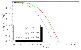
Figure 1: Quark condensate as a function of the temperature and the isospin chemical potential

Figure 1 shows the chiral condensate at finite temperature and isospin chemical potential. It is interesting to remark that the chiral condensate vanishes also, almost linearly with the baryonic density Peng:2003nq .

The introduction of isospin chemical potential breaks the degeneracy of the thermal evolution of the pion masses and decay constants Loewe:2002tw . This suggests considering the G-MOR relation in terms of the average value for the masses and decay constants. In fact, using our results from the above quoted paper we find that

$$\overline{m}_{\pi}^{2}\overline{f}_{\pi}^{2}=-\textstyle{\frac{1}{2}}(m_{u}+m_{d})\langle\!\langle\sigma\rangle\!\rangle.$$ (21)

where

$$\overline{m}_{\pi} \equiv \textstyle{\frac{1}{3}}\left(m_{\pi^{+}}+m_{\pi^{-}}+m_{\pi^{0}}\right),$$ (22)

$$\overline{f}_{\pi} \equiv \textstyle{\frac{1}{3}}\left(f_{\pi^{+}}+f_{\pi^{-}}+f_{\pi^{0}}\right).$$ (23)

With this prescription for the G-MOR relation, we can consider $\tilde{h}_{1}=\frac{1}{3}\epsilon_{ud}^{2}l_{7}\sim 0$.

III.2 Isospin number density.

The isospin number density condensate gives us information about the baryon number difference between $u$ and $d$ quarks in the thermal or populated vacuum. The isospin number density is defined as the 0-Lorentz component and third-isospin component of the vector current

$$\langle\!\langle n_{I}\rangle\!\rangle\equiv\langle\!\langle 0|\textstyle{\frac{1}{2}}q^{\dagger}\tau^{3}q|0\rangle\!\rangle=\langle\!\langle 0|V_{0}^{3}|0\rangle\!\rangle.$$ (24)

We need to calculate the expectation value of the vector current in the vacuum. We will see that the only non-vanishing component of the vector current in the vacuum is the isospin number density. In fact, by considering the expansion of the vector current and using the fact that $\langle\!\langle 0|\pi_{a}|0\rangle\!\rangle=0$ and $\langle\!\langle 0|\pi_{a\neq 3}\pi_{3}|0\rangle\!\rangle=0$ we find in the first phase case

$$\langle\!\langle 0|\bm{V}_{(1,2)\mu}|0\rangle\!\rangle=\langle\!\langle 0|-i(\pi_{\mbox{\tiny$+$}}\partial_{\mu}\pi_{\mbox{\tiny$-$}}-\pi_{\mbox{\tiny$-$}}\partial_{\mu}\pi_{\mbox{\tiny$+$}})\\ +2\mu_{\mbox{\tiny I}}|\pi|^{2}u_{\mu}|0\rangle\!\rangle{\bf e}_{3}.$$ (25)

This means that the isospin-number density depends on temperature only through thermal insertions in loop corrections, and therefore, vanishes for $T=0$ or $|\mu_{\mbox{\tiny I}}|=0$. Using the fact that

$$\langle\!\langle 0|\pi^{a}(x)\partial\pi^{b}(x)|0\rangle\!\rangle=\Big{[}\partial_{y}\langle\!\langle 0|T\pi^{a}(x)\pi^{b}(y)|0\rangle\!\rangle\Big{]}_{y=x},$$ (26)

we find that the vacuum expectation value of the vector current is oriented in the ${\bf e}_{3}$ direction and proportional to the fourth velocity: $\langle\!\langle 0|\bm{V}_{\mu}|0\rangle\!\rangle=\langle\!\langle n_{I}\rangle\!\rangle u_{\mu}{\bf e}_{3}$. The isospin number density condensate is then.

$$\langle\!\langle n_{I}\rangle\!\rangle=8mf^{2}\alpha\epsilon(\mu_{\mbox{\tiny I}})J,$$ (27)

where $J$ is a function of $T,\mu_{\mbox{\tiny I}}$ defined in the Appendix. A finite value of this condensate requires a finite value for both, $\mu_{\mbox{\tiny I}}$ and $T$, as can be seen in fig. 2

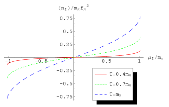
Figure 2: Isospin-number density condensate as a function of the isospin chemical potential for different values of the temperature.

IV Second phase: $|\mu_{\mbox{\tiny I}}|\gtrsim m$

In this phase, due to the non trivial vacuum expectation value of the $U$ fields mentioned in eq. (8), a condensation of pions, in this case of negative pion, occurs, giving rise to a superfluid phase. The apparition of two new condensates, the pion condensate and the axial-charge density condensate will break parity.

As we mentioned before in section I, we can expand the loop corrections in this region as a series of powers of $s^{2}=1-\frac{m^{4}}{\mu_{\mbox{\tiny I}}^{4}}$. The condensates will have the shape

$$\langle\!\langle J\rangle\!\rangle=\langle J\rangle\bigg{\{}\eta(s)+\alpha^{\prime}\sum_{n=0}\sigma_{n}(T/|\mu_{\mbox{\tiny I}}|)s^{2n}\bigg{\}}$$ (28)

IV.1 Chiral condensate

Following the same procedure we used in the case of the first phase, the non-vanishing components of the chiral condensate at order $s^{0}$ are

$$J_{s(1,0)} = -2Bf^{2}c,$$ (29)

$$J_{s(1,2)} = Bc\big{[}\pi_{0}^{2}+2|\tilde{\pi}|^{2}\big{]},$$ (30)

$$J_{s(3,0)} = -4B\mu_{\mbox{\tiny I}}^{2}c[l_{3}+l_{4}+\tilde{h}_{1}+{\cal O}(s^{2})].$$ (31)

The term $c$ must be kept because it is a global constant.

The resulting chiral condensate at finite temperature and isospin chemical potential is then

$$\langle\!\langle\sigma\rangle\!\rangle=-2Bf^{2}c\big{\{}1+\alpha^{\prime}\big{[}-\textstyle{\frac{1}{2}}\bar{l}_{3}+2\bar{l}_{4}-2I^{\prime}_{0}-4I^{\prime}\big{]}\big{\}}.$$ (32)

In Fig. 3, we can see the transition of the chiral condensate from the first phase to the second phase. Now, the chiral condensate in the second phase tends to decrease abruptly with the chemical potential. This effect is enhanced by temperature. Keeping in mind the previous section, we can set the constant $\tilde{h}_{1}\sim 0$ if the G-MOR relation is valid.

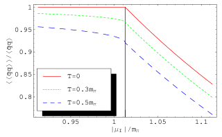
Figure 3: Chiral condensate as a function of the isospin chemical potential for different values of the temperature. The vertical line denotes the transition point between the two phases.

IV.2 Isospin-number density.

The non-vanishing components of the condensed vector current at order $s^{0}$ in the loop corrections are

$$\langle\!\langle 0|\bm{V}_{\mu}|0\rangle\!\rangle_{(1,0)} = -f^{2}|\mu_{\mbox{\tiny I}}|s^{2}u_{\mu}{\bf e}_{3},$$ (33)

$$\langle\!\langle 0|\bm{V}_{\mu}|0\rangle\!\rangle_{(1,2)} = \langle\!\langle 0|-i(\tilde{\pi}_{1}\partial_{\mu}\tilde{\pi}_{2}-\tilde{\pi}_{2}\partial_{\mu}\tilde{\pi}_{1})$$ (34)

$$-2|\mu_{\mbox{\tiny I}}||\tilde{\pi}|^{2}u_{\mu}+|\mu_{\mbox{\tiny I}}|^{3}{\cal O}(s^{2})|0\rangle\!\rangle{\bf e}_{3}.$$

Like in the firs phase, the vacuum expectation value of the vector current will be oriented as $\langle\!\langle 0|\bm{V}_{\mu}|0\rangle\!\rangle=\langle\!\langle n_{I}\rangle\!\rangle u_{\mu}{\bf e}_{3}$. The isospin number density condensate at finite temperature and chemical potential is then

$$\langle\!\langle n_{I}\rangle\!\rangle=-|\mu_{\mbox{\tiny I}}|f^{2}\big{\{}s^{2}+8\alpha^{\prime}J^{\prime}\big{\}}.$$ (35)

In fig. 4, we can see the transition of the isospin number density from the first phase to the second phase. Like the chiral condensate, in the second phase $\langle\!\langle n_{I}\rangle\!\rangle$ tends to decrease abruptly with the chemical potential. Once again this effect is enhanced by temperature.

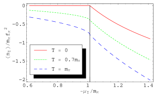
Figure 4: Isospin number density as a function of the isospin chemical potential for different values of the temperature.

IV.3 Pion condensate.

Now, in the second phase, the pion condensate is finite and provides us important information about the condensed phase. The pion condensate is defined as

$$\langle\!\langle\pi^{a}\rangle\!\rangle\equiv\langle\!\langle 0|i\bar{q}\gamma_{5}\tau^{a}q|0\rangle\!\rangle=\langle\!\langle 0|J_{p}^{a}|0\rangle\!\rangle,$$ (36)

and carry the same quantum numbers of the pion field. The non-vanishing components of the pion condensates are

$$\bm{J}_{p(1,0)} = -2Bf^{2}s\tilde{\bf e}_{1},$$ (37)

$$\bm{J}_{p(1,2)} = Bs\big{[}\pi_{0}^{2}+2|\pi|^{2}\big{]}\tilde{\bf e}_{1},$$ (38)

$$\bm{J}_{p(3,0)} = -4B\mu_{\mbox{\tiny I}}^{2}s[l_{3}+l_{4}+{\cal O}(s^{2})]\tilde{\bf e}_{1}.$$ (39)

As we did for the chiral condensate, we must keep the term $s$, since it is a global factor. We can see that the pion condensate is oriented in the direction $\tilde{\bf e}_{1}$, i.e., $\langle\!\langle\bm{\pi}\rangle\!\rangle=\langle\!\langle\tilde{\pi}_{1}\rangle\!\rangle\tilde{\bf e}_{1}$.

Proceeding in the same way as we did with the other condensates, the pion condensate at finite temperature and isospin chemical potential is

$$\langle\!\langle\tilde{\pi}_{1}\rangle\!\rangle=2Bf^{2}s\{1+\alpha^{\prime}[-\textstyle{\frac{1}{2}}\bar{l}_{3}+2\bar{l}_{4}-2I^{\prime}_{0}-4I^{\prime}]\}.$$ (40)

It is important to recall that the pion condensates, like the chiral condensate, give an information about the quarks condensed in the vacuum; in this case the pion condensate is a mixture of $\bar{u}\gamma_{5}d$ and $\bar{d}\gamma_{5}u$. Although related, do not confuse the pion condensate with the number density of condensed pions.

Note that this result is basically the same as the chiral condensate (except the global factors $s$ and $-c$) if we neglect the term $\tilde{h}_{1}$. Then the chiral condensate and pion condensate satisfy the relation

$$s\langle\!\langle\sigma\rangle\!\rangle+c\langle\!\langle\tilde{\pi}_{1}\rangle\!\rangle=0.$$ (41)

We will see that this relation is valid in the limit when $|\mu_{\mbox{\tiny I}}|\gg m$.

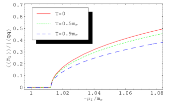
Figure 5: Pion condensate as a function of the isospin chemical potential for different values of the temperature. The vertical line denotes the transition point between the two phases.

Fig. 5 shows the behavior of the pion condensate as function of $\mu_{\mbox{\tiny I}}$ for different values of $T$. If we compare with fig. 3, we can see that the chiral condensate diminishes with the chemical potential in a similar rate as the pion condensate increases, according to eq. (41). This suggests that the quarks in the chiral condensate may mix together to form a mixed $u$-$d$ pseudo-scalar Cooper-pairs state. Because of the thermal bath, both chiral and pion condensates decrease as a function of $T$, as expected, due to the increase of the $\pi^{-}$ mass in the thermal bath.

IV.4 Axial-isospin charge density (AICD) condensate

The second phase supports also another condensate, the axial-isospin charge density condensate, defined as

$$\langle\!\langle{\cal Q}_{A}^{a}\rangle\!\rangle=\langle\!\langle 0|\textstyle{\frac{1}{2}}q^{\dagger}\gamma_{5}\tau^{a}q|0\rangle\!\rangle=\langle\!\langle 0|A_{0}^{a}|0\rangle\!\rangle$$ (42)

The non-vanishing components of the effective axial current, according to the chiral approach, in the vacuum at the lowest order in the $s$ expansion are

$$\langle\!\langle 0|\bm{A}_{\mu(1,0)}|0\rangle\!\rangle = f^{2}|\mu_{\mbox{\tiny I}}|cs\tilde{\bf e}_{2},$$ (43)

$$\langle\!\langle 0|\bm{A}_{\mu(1,2)}|0\rangle\!\rangle = -|\mu_{\mbox{\tiny I}}|cs\langle\!\langle 0|\frac{i}{|\mu_{\mbox{\tiny I}}|}(\tilde{\pi}_{+}\partial_{\mu}\tilde{\pi}_{-}-\tilde{\pi}_{-}\partial_{\mu}\tilde{\pi}_{+})$$ (44)

$$\quad+\pi_{0}^{2}+3|\pi|^{2}+\mu_{\mbox{\tiny I}}^{2}{\cal O}(s^{2})|0\rangle\!\rangle\tilde{\bf e}_{2},$$

$$\langle\!\langle 0|\bm{A}_{\mu(3,0)}|0\rangle\!\rangle = |\mu_{\mbox{\tiny I}}|^{3}cs[2l_{4}+{\cal O}(s^{2})].$$ (45)

Note that this axial-charge density is oriented in the $\tilde{\bf e}_{2}$ direction:$\langle\!\langle 0|\bm{A}_{\mu}|0\rangle\!\rangle=\langle\!\langle{\cal\tilde{Q}}_{A}^{2}\rangle\!\rangle u_{\mu}\tilde{\bf e}_{2}$, perpendicular to the orientation of the pion condensate and also with respect to the Vector-current vacuum expectation value. The three previous condensates are a basis in the isospin $SU(2)$ space. The AICD condensate is then

$$\langle\!\langle{\cal\tilde{Q}}_{A}^{2}\rangle\!\rangle=f^{2}cs[1+\alpha^{\prime}(2\bar{l}_{4}-4I^{\prime}-4I^{\prime}_{0}-8J^{\prime})].$$ (46)

Fig. 6 shows the behavior of the AICD condensate as function of temperature and $\mu_{\mbox{\tiny I}}$. Note that at a certain critical temperature, for growing values of $\mu_{\mbox{\tiny I}}$, the AICD condensate changes its sign. We would like to remark that this object seems to be a very interesting order parameter for the phase transition into the pion superfluid phase. Perhaps lattice measurements could confirm this point.

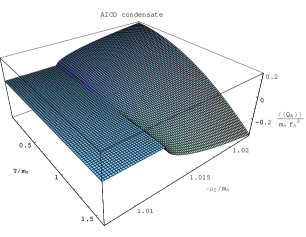
Figure 6: Axial-Isospin charge density condensate, scaled with $m_{\pi}f_{\pi}^{2}$, plotted in the neighborhood of the phase transition as function of temperature and isospin chemical potential, scaled both with $m_{\pi}$.

V Second phase: $|\mu_{\mbox{\tiny I}}|\gg m$

When $|\mu_{\mbox{\tiny I}}|\gg m$, the natural expansion parameter is $c=\frac{m^{2}}{\mu_{\mbox{\tiny I}}^{2}}$. So the different objects will be expressed as power series of the form

$$\langle\!\langle J\rangle\!\rangle=\langle J\rangle\bigg{\{}\eta(c)+\alpha^{\prime}\sum_{n=0}\big{[}\sigma_{n}(T/|\mu_{\mbox{\tiny I}}|)+\sigma^{\mbox{\tiny log }}_{n}\ln{c}\big{]}c^{n}\bigg{\}}.$$ (47)

The main difference between the previous equation and eq. (28) is the presence of logarithms since loop corrections give rise to terms of the form $\lambda-\ln(\mu_{\mbox{\tiny I}}^{2}/\Lambda^{2})$, which cancel with the terms $\lambda-\ln(m^{2}/\Lambda^{2})$ coming from the $l_{i}$ coupling constants. These logarithms turn out to be extremely important for the behavior of the condensates in this region.

V.1 Chiral condensate

The non-vanishing components of the chiral condensate, neglecting higher corrections of order $c^{2}$, are

$$\langle\!\langle 0|J_{s}|0\rangle\!\rangle_{(1,0)} = -2Bf^{2}c,$$ (48)

$$\langle\!\langle 0|J_{s}|0\rangle\!\rangle_{(1,2)} = Bc\langle\!\langle 0|\pi_{0}^{2}+\tilde{\pi}_{1}^{2}+\tilde{\pi}_{2}^{2}|0\rangle\!\rangle,$$ (49)

$$\langle\!\langle 0|J_{s}|0\rangle\!\rangle_{(3,0)} = -2B\mu_{\mbox{\tiny I}}^{2}c[l_{4}+2\tilde{h}_{1}+{\cal O}(c^{2})],$$ (50)

keeping the global term $c$. Following the same procedure as in the previous chapters, the chiral condensate at finite temperature and isospin chemical potential is

$$\langle\!\langle\sigma\rangle\!\rangle=-2Bf^{2}c\bigg{\{}1+\alpha^{\prime}\bigg{[}\bar{l}_{4}+32\pi^{2}\tilde{h}_{1}\\ +2\ln c-4I^{\prime}_{0}-\textstyle{\frac{2}{3}}\left(\textstyle{\frac{\pi T}{\mu_{\mbox{\tiny I}}}}\right)^{2}\bigg{]}\bigg{\}}.$$ (51)

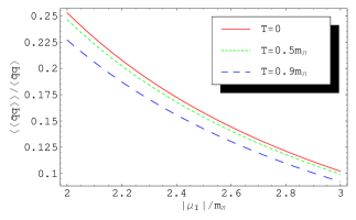
Figure 7: Chiral condensate as a function of the isospin chemical potential for different values of the temperature for high values of the chemical potential.

Fig. 7 shows the chiral condensate behavior at finite temperature for high values of the chemical potential. It has a decreasing behavior as function of both parameters.

V.2 Isospin number density.

The non-vanishing components of the vector current, within the thermal vacuum, neglecting higher corrections of order $c^{2}$, are

$$\langle\!\langle 0|\bm{V}_{\mu}|0\rangle\!\rangle_{(1,0)} = -|\mu_{\mbox{\tiny I}}|f^{2}s^{2}u_{\mu}{\bf e}_{3},$$ (52)

$$\langle\!\langle 0|\bm{V}_{\mu}|0\rangle\!\rangle_{(1,2)} = |\mu_{\mbox{\tiny I}}|s^{2}\langle\!\langle 0|\pi_{0}^{2}+\tilde{\pi}_{1}^{2}+\mu_{\mbox{\tiny I}}^{2}{\cal O}(c^{2})|0\rangle\!\rangle u_{\mu}{\bf e}_{3},$$

$$\langle\!\langle 0|\bm{V}_{\mu}|0\rangle\!\rangle_{(3,0)} = -4|\mu_{\mbox{\tiny I}}|^{3}s^{2}\big{[}l_{1}+l_{2}+{\cal O}(c^{2})\big{]}u_{\mu}{\bf e}_{3}.$$ (54)

The isospin number density is then

$$\langle\!\langle n_{I}\rangle\!\rangle=-|\mu_{\mbox{\tiny I}}|f^{2}s^{2}\left\{1+2\alpha^{\prime}\left[\textstyle{\frac{1}{3}}\bar{l}_{1}+\textstyle{\frac{2}{3}}\bar{l}_{2}+2\ln c-4I^{\prime}_{0}\right]\right\}.$$ (55)

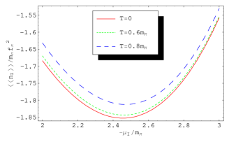
Figure 8: Isospin-number density as a function of the isospin chemical potential at different values of the temperature in the high chemical potential limit.

Fig. 8 shows the isospin number density for different temperatures and high values of the isospin chemical potential. Due to the logarithmic term, it starts to grow again with the chemical potential. As in the case of the $\pi^{+}$ mass in this high chemical potential limit, it grows with temperature, in contrast to the $|\mu_{\mbox{\tiny I}}|\sim m$ case. A crossover of the different temperature lines must occur somewhere in the intermediate region of the chemical potential. At this point, however, we must proceed with care since two loop corrections could provide us with other logarithmic terms that may change the shape of this curve. In the previous case, close to the phase transition point, we do not have such difficulties to deal with.

V.3 Pion condensate

The non-vanishing components of the pseudo-scalar current, within the thermal vacuum and neglecting higher corrections of order $c^{2}$, are

$$\bm{J}_{p(1,0)} = 2Bf^{2}s\tilde{\bf e}_{1},$$ (56)

$$\bm{J}_{p(1,2)} = -Bs\big{[}\pi_{0}^{2}+\tilde{\pi}_{1}^{2}+\tilde{\pi}_{2}^{2}\big{]}\tilde{\bf e}_{1},$$ (57)

$$\bm{J}_{p(3,0)} = 2\mu_{\mbox{\tiny I}}^{2}Bs\big{[}l_{4}+{\cal O}(c^{2})\big{]}\tilde{\bf e}_{1}.$$ (58)

The pion condensate is then

$$\langle\!\langle\tilde{\pi}_{1}\rangle\!\rangle=2Bf^{2}s\bigg{\{}1+\alpha^{\prime}\bigg{[}\bar{l}_{4}+2\ln c-4I^{\prime}_{0}-\left(\textstyle{\frac{\pi T}{\mu_{\mbox{\tiny I}}}}\right)^{2}\bigg{]}\bigg{\}}.$$ (59)

Fig. 9 shows the pion condensate at finite temperature and high values of the chemical potential. Like the isospin number density, it has a deflection and starts to decrease, due to the logarithmic terms. Again in this case, we must be careful since as in the isospin number density evolution, new important logarithmic terms, from two-loop calculations, could also change the bending as well as the general shape of our one-loop result. Comparing with equation (51), if we neglect the term $\tilde{h}_{1}$, the pion condensate and the chiral condensate follow the relation $s\langle\!\langle\sigma\rangle\!\rangle+c\langle\!\langle\tilde{\pi}_{1}\rangle\!\rangle=0$, as was the case in the region $|\mu_{\mbox{\tiny I}}|\gtrsim m$.

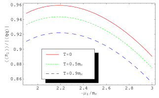
Figure 9: Pion condensate as a function of the isospin chemical potential for different temperatures in the limit of high chemical potential.

V.4 AICD condensate

The axial-vector current components, neglecting higher terms in the expansion in terms of $c^{n}$ are

$$\bm{A}_{\mu(1,0)} = f^{2}|\mu_{\mbox{\tiny I}}|csu_{\mu}\tilde{\bf e}_{2},$$ (60)

$$\bm{A}_{\mu(1,2)} = |\mu_{\mbox{\tiny I}}|cs\bigg{[}\frac{1}{|\mu_{\mbox{\tiny I}}|c}(\tilde{\pi}_{1}\partial_{\mu}\tilde{\pi}_{2}-\tilde{\pi}_{2}\partial_{\mu}\tilde{\pi}_{1})$$ (61)

$$\hskip 62.59596pt-\pi_{0}^{2}-2\tilde{\pi}_{1}^{2}-\tilde{\pi}_{2}^{2}\bigg{]}\tilde{\bf e}_{2}$$

$$\bm{A}_{\mu(3,0)} = |\mu_{\mbox{\tiny I}}|^{3}cs2\big{[}l_{1}+l_{2}+{\cal O}(c^{2})\big{]}u_{\mu}\tilde{\bf e}_{2},$$ (62)

where we keep the term $cs$ as a global factor. In this case we use also the propagator $D_{DJ}(p)_{12}$ which is of order $c$. The factor $1/c$ in eq. (61) cancels the other term $c$ of the propagator, so our result is still of ${\cal O}(c^{0})$. As int the case $|\mu_{\mbox{\tiny I}}|\gtrsim m$, the AICD condensate will be oriented in the $u_{\mu}\tilde{\bf e}_{3}$ direction. The AICD condensate is then

$$\langle\!\langle{\cal\tilde{Q}}_{A}^{2}\rangle\!\rangle=f^{2}cs\bigg{\{}1+\alpha^{\prime}\bigg{[}\textstyle{\frac{2}{3}}\bar{l}_{1}+\textstyle{\frac{4}{3}}\bar{l}_{2}+2\ln c-\textstyle{\frac{1}{2}}\\ -12I^{\prime}_{0}+I^{\prime}_{1}-\textstyle{\frac{2}{3}}\left(\textstyle{\frac{\pi T}{\mu_{\mbox{\tiny I}}}}\right)^{2}-\textstyle{\frac{32}{15}}\left(\textstyle{\frac{\pi T}{\mu_{\mbox{\tiny I}}}}\right)^{4}\bigg{]}\bigg{\}}.$$ (63)

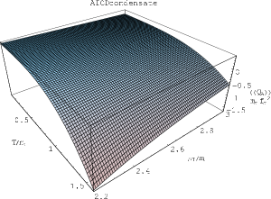
Figure 10: Axial-Isospin charge density condensate, scaled with $m_{\pi}f_{\pi}^{2}$, plotted for high values of $\mu_{\mbox{\tiny I}}$, as function of temperature and isospin chemical potential, scaled both with $m_{\pi}$.

Fig. 10 shows the behavior of the AICD condensate for high values of $\mu_{\mbox{\tiny I}}$. Due to the logarithmic term, the condensate for high $T$ values starts to grow again as function of $\mu_{\mbox{\tiny I}}$.

VI Final comments and summary

It is interesting to remark that our pion condensate behaves as the diquark condensate, according to the lattice QCD analysis, as function of temperature and isospin chemical potential Kogut:2002tm ; Kogut:2002zg . This condensate starts to rise as soon as we go into the second phase, close to the phase transition point Kogut:2001if ; Kogut:2002cm . However, for bigger values of $\mu_{\mbox{\tiny I}}$ it decreases, in agreement with our analytical results which show a decreasing behavior as $\sim\ln 1/\mu_{\mbox{\tiny I}}^{2}$. The lattice analysis has confirmed also the relation between the chiral condensate and the pion condensate according to eq. (41). The chiral condensate and the isospin number density also agree with the lattice results.

We would like to emphasize that the G-MOR relation (at least in the first phase) remains valid if we write it in terms of the average values of the pion masses and decay constants. Also the relation $s\langle\!\langle\sigma\rangle\!\rangle+c\langle\!\langle\tilde{\pi}_{1}\rangle\!\rangle=0$ is confirmed lattice results Kogut:2002cm .

Finally, we think that the realization of condensates as a basis in the isospin space in the second phase ($\langle\!\langle\bm{A}_{0}\rangle\!\rangle$, $\langle\!\langle\bm{V}_{0}\rangle\!\rangle$, $\langle\!\langle\bm{J}_{p}\rangle\!\rangle$ are all perpendicular) is a very interesting phenomenon. One-loop thermal corrections do not destroy this property, which remains valid when $|\mu_{\mbox{\tiny I}}|\gtrsim m$ as well as when $|\mu_{\mbox{\tiny I}}|\gg m$.

Acknowledgements

The work of M.L. and C.V. have been supported by Fondecyt (Chile) under grant No.1010976.

APPENDIX

The functions involved in the radiative corrections in the first phase are

$$\alpha\! = \!(m/4\pi f)^{2}$$

$$I = \int_{1}^{\infty}\!\!\!dx\sqrt{x^{2}-1}[n_{B}(mx-|\mu_{\mbox{\tiny I}}|)+n_{B}(mx+|\mu_{\mbox{\tiny I}}|)]$$

$$J\! = \!\int_{1}^{\infty}\!\!\!dxx\sqrt{x^{2}-1}[n_{B}(mx-|\mu_{\mbox{\tiny I}}|)-n_{B}(mx+|\mu_{\mbox{\tiny I}}|)]$$

$$I_{n}\! = \!\int_{1}^{\infty}\!\!\!dxx^{2n}\sqrt{x^{2}-1}~{}2n_{B}(mx)$$

being $\alpha$ the perturbative parameter. These integrals do not depend on the chemical potential sign, and grow with both, temperature and chemical potential.

In the case of the second phase, we denote the same functions with a prime: $\alpha^{\prime}$, $I^{\prime}$, $J^{\prime}$, $I^{\prime}_{n}$ which are the same functions, but with $|\mu_{\mbox{\tiny I}}|$ instead of $m$.

$$\alpha^{\prime}\! = \!\!(\mu_{\mbox{\tiny I}}/4\pi f)^{2}$$

$$I^{\prime}\! = \!\!\int_{1}^{\infty}\!\!\!dx\sqrt{x^{2}-1}\big{[}n_{B}\big{(}|\mu_{\mbox{\tiny I}}|(x\!-\!1)\big{)}+n_{B}\big{(}|\mu_{\mbox{\tiny I}}|(x\!+\!1)\big{)}\big{]}$$

$$J^{\prime}\! = \!\!\int_{1}^{\infty}\!\!\!dxx\sqrt{x^{2}-1}\big{[}n_{B}\big{(}|\mu_{\mbox{\tiny I}}|(x\!-\!1)\big{)}-n_{B}\big{(}|\mu_{\mbox{\tiny I}}|(x\!+\!1)\big{)}\big{]}$$

$$I^{\prime}_{n}\! = \!\!\int_{1}^{\infty}\!\!\!dxx^{2n}\sqrt{x^{2}-1}~{}2n_{B}(|\mu_{\mbox{\tiny I}}|x).$$

These integrals are also growing functions of the temperature but decrease with the chemical potential.

References

• (1) M. Loewe and C. Villavicencio, Phys. Rev. D67, 074034 (2003), hep-ph/0212275.
• (2) M. Loewe and C. Villavicencio, Phys. Rev. D70, 074005 (2004), hep-ph/0404232.
• (3) J. B. Kogut, M. A. Stephanov, and D. Toublan, Phys. Lett. B464, 183 (1999), hep-ph/9906346.
• (4) J. B. Kogut, M. A. Stephanov, D. Toublan, J. J. M. Verbaarschot, and A. Zhitnitsky, Nucl. Phys. B582, 477 (2000), hep-ph/0001171.
• (5) D. T. Son and M. A. Stephanov, Phys. Rev. Lett. 86, 592 (2001), hep-ph/0005225.
• (6) J. B. Kogut and D. Toublan, Phys. Rev. D64, 034007 (2001), hep-ph/0103271.
• (7) J. B. Kogut and D. K. Sinclair, Phys. Rev. D66, 014508 (2002), hep-lat/0201017.
• (8) J. B. Kogut and D. K. Sinclair, Phys. Rev. D66, 034505 (2002), hep-lat/0202028.
• (9) J. B. Kogut, D. Toublan, and D. K. Sinclair, Phys. Lett. B514, 77 (2001), hep-lat/0104010.
• (10) J. B. Kogut, D. Toublan, and D. K. Sinclair, Nucl. Phys. B642, 181 (2002), hep-lat/0205019.
• (11) A. Barducci, G. Pettini, L. Ravagli, and R. Casalbuoni, Phys. Lett. B564, 217 (2003), hep-ph/0304019.
• (12) D. Toublan and J. B. Kogut, Phys. Lett. B564, 212 (2003), hep-ph/0301183.
• (13) M. Frank, M. Buballa, and M. Oertel, Phys. Lett. B562, 221 (2003), hep-ph/0303109.
• (14) A. Barducci, R. Casalbuoni, G. Pettini, and L. Ravagli, Phys. Rev. D69, 096004 (2004), hep-ph/0402104.
• (15) A. Barducci, R. Casalbuoni, G. Pettini, and L. Ravagli, Phys. Rev. D71, 016011 (2005), hep-ph/0410250.
• (16) L. He and P. Zhuang, (2005), hep-ph/0501024.
• (17) J. Gasser and H. Leutwyler, Ann. Phys. 158, 142 (1984).
• (18) K. Splittorff, D. Toublan, and J. J. M. Verbaarschot, Nucl. Phys. B620, 290 (2002), hep-ph/0108040.
• (19) K. Splittorff, D. Toublan, and J. J. M. Verbaarschot, Nucl. Phys. B639, 524 (2002), hep-ph/0204076.
• (20) C. A. Dominguez, M. S. Fetea, and M. Loewe, Phys. Lett. B387, 151 (1996), hep-ph/9608396.
• (21) G. X. Peng, M. Loewe, U. Lombardo, and X. J. Wen, Nucl. Phys. B (Proc. Suppl). 133, 259 (2004), hep-ph/0309304.