Displacement Operator Formalism for Renormalization
and Gauge Dependence to All Orders

Abstract

We present a new method for determining the renormalization of Green functions to all orders in perturbation theory, which we call the displacement operator formalism, or the $D$-formalism, in short. This formalism exploits the fact that the renormalized Green functions may be calculated by displacing by an infinite amount the renormalized fields and parameters of the theory with respect to the unrenormalized ones. With the help of this formalism, we are able to obtain the precise form of the deformations induced to the Nielsen identities after renormalization, and thus derive the exact dependence of the renormalized Green functions on the renormalized gauge-fixing parameter to all orders. As a particular non-trivial example, we calculate the gauge-dependence of $\tan\beta$ at two loops in the framework of an Abelian Higgs model, using a gauge-fixing scheme that preserves the Higgs-boson low-energy theorem for off-shell Green functions. Various possible applications and future directions are briefly discussed.

I Introduction

Renormalization is of central importance in quantum field theory Schwinger:1948iu ; Feynman:1948fi ; Dyson:1949bp ; Bogoliubov:1957gp ; Hepp:1966eg ; Zimmermann:1969jj ; Symanzik:1970rt ; Epstein:1973gw ; 'tHooft:1972fi ; 'tHooft:1971fh ; Lee:1974zg ; Becchi:1974md , and its consistent implementation has been crucial for the advent and success of gauge theories in general, and of the Standard Model of strong and electroweak interactions in particular. Despite half a century of practice, however, renormalization remains a delicate procedure, mainly because it interferes non-trivially with the fundamental symmetries encoded in the Lagrangian defining the theory. The subtleties involved manifest themselves at almost every step, ranging from the necessity to employ regularization methods respecting all relevant symmetries, the need for renormalization schemes that do not spoil the important constraints imposed by the symmetries on the Green functions of the theory, all the way to the practical, book-keeping challenges appearing when the renormalization is carried out in higher order calculations.

In this paper we develop a new formalism, which we call the Displacement Operator Formalism, or the $D$-formalism, in short. The $D$-formalism enables one to systematically organize and explicitly compute the counterterms (CTs) involved in the renormalization procedure, to all orders in perturbation theory. The central observation, leading to this new formulation, is that the effect of renormalizing any given Green function may be expressed in terms of ultraviolet (UV) infinite displacements caused by the renormalization on both the fields and the parameters of the theory. Specifically, these UV infinite displacements, or shifts, quantify the difference between fields and parameters before and after renormalization. For example, in the case of a theory with a scalar field $\phi$, and two parameters, the coupling constant $\lambda$ and the squared mass $m^{2}$, the corresponding UV infinite shifts $\delta\phi$, $\delta\lambda$, and $\delta m^{2}$ are given by $\delta\phi=(Z_{\phi}^{\frac{1}{2}}-1)\phi_{\mathrm{R}}$, $\delta\lambda=(Z_{\lambda}-1)\lambda_{\mathrm{R}}$, and $\delta m^{2}=(Z_{m^{2}}-1)\,m^{2}_{R}$, where the renormalization constants are defined, as usual, through $\phi=Z_{\phi}^{\frac{1}{2}}\phi_{\mathrm{R}}$, $\lambda=Z_{\lambda}\lambda_{\mathrm{R}}$, and $m^{2}=Z_{m^{2}}\,m^{2}_{\rm R}$. Evidently, in this formulation, dynamical fields and parameters are treated on a completely equal footing.

In order to systematically expose the way in which these shifts implement the renormalization at the level of Green functions, one introduces the displacement operator $D$, a differential operator given by $D=\delta\phi\frac{\partial}{\partial\phi_{\mathrm{R}}}+\delta\lambda\frac{\partial}{\partial\lambda_{\mathrm{R}}}+\delta m^{2}\frac{\partial}{\partial m_{\mathrm{R}}^{2}}$. It turns out (see section II for details) that the net renormalization effect is captured to all orders by the exponentiation of the $D$ operator. Thus, the renormalized ($n$-point) Green functions $\Gamma_{\phi^{n}}^{\mathrm{R}}$ are eventually obtained from the bare ones, $\Gamma_{\phi^{n}}$, through the master equation $\phi^{n}_{\mathrm{R}}\Gamma_{\phi^{n}}^{\mathrm{R}}=\langle e^{D}(\phi^{n}_{\mathrm{R}}\Gamma_{\phi^{n}})\rangle$, where the brackets $\langle\dots\rangle$ means that the corresponding shifts, implicit in the $D$ operator, are to be replaced by their expressions in terms of the renormalization constants given above, after the end of the differentiation procedure.

It is important to appreciate at this point the inherent non-perturbative nature of the above formulation, manifesting itself through the exponentiation of the $D$ operator. Perturbative results (at arbitrary order) may be recovered as a special case through an appropriate order-by-order expansion of the above master formula, whose validity however is not restricted to the confines of perturbation theory. This is to be contrasted with other well-known renormalization methods (as, for example, the “algebraic approach” Piguet:1995er ; Kraus:1997bi ; Grassi:1999tp ), which are formulated at the perturbative level.

One of the main advantages of this formulation is the ability it offers in determining unambiguously the CTs to any given order in perturbation theory. Specifically, the contributions of the CTs are automatically obtained through the straightforward application of the $D$ operator on the unrenormalized Green functions, without having to resort to any additional arguments whatsoever. This last point is best appreciated in the context of complicated non-Abelian gauge theories, or special gauge-fixing schemes, where keeping track of the CTs can be not only logistically demanding, but at times also conceptually subtle. For example, possible ambiguities related to the gauge-fixing parameter (GFP) renormalization, endemic in sophisticated quantization schemes such as the Background Field Method (BFM) Dewitt:ub ; 'tHooft:vy ; Abbott:1980hw ; Capper:1982tf ; Abbott:zw are automatically resolved (see section III). As we will see in detail in the main body of the paper, the fact that the $D$-formalism correctly incorporates the action of the CTs is clearly reflected in the absence of overlapping divergences from the resulting expressions.

An important property of the $D$-formalism is that it reproduces exactly the usual diagrammatic representation of the CTs, if one acts with the $D$ operator on the Feynman graphs determining the given Green function before the integration over the virtual loop momenta is carried out. If one instead acts with $D$ after the momentum integration has been performed one loses this direct diagrammatic interpretation, but recovers the same final answer for the renormalized Green function. This last point becomes particularly relevant in the case of gauge theories, where one of the parameters that undergoes renormalization is the GFP, to be denoted by $\xi$. This, in turn, will introduce in the $D$ operator a term of the form $\delta\xi\frac{\partial}{\partial\xi_{\mathrm{R}}}$, which must act on the corresponding Green function. Clearly, for this to become possible the dependence of the Green function on $\xi$ must be kept arbitrary, that is, one may not choose a convenient value for $\xi$, like for example $\xi=1$. Evidently, if one were to first carry out the momentum integration and then differentiate, one would be faced with the book-keeping complications of computing with an arbitrary $\xi$. If, instead, one opts for the action of $D$ on the Green function before the loop integration, the straightforward use of the chain rule for the strings of tree-level propagators (and possibly vertices), and a subsequent choice of, say, $\xi=1$, is completely equivalent to the conventional approach of computing at a fixed gauge. Obviously, one may choose either one of the two procedures, i.e., integrate before or after the action of $D$, depending on the specific problem at hand, a fact which exemplifies the versatility of the new formalism.

Perhaps one of the most powerful features of the $D$-formalism consists in the fact that it provides a handle on the structure and organization of the CTs to all orders in perturbation theory. In particular, it furnishes the exact form of the deformations induced due to the renormalization procedure to any type of relations or constraints which are valid at the level of unrenormalized Green functions. Such deformations will arise in general if the symmetries (global or local) enforcing the relations in question involve static parameters, which cannot admit kinetic terms compatible with those symmetries. A well-known example of such a type of relation is the so-called Nielsen identities (NI) Nielsen:1975ph , which, by virtue of the extended Becchi–Rouet–Stora ($e$BRS) symmetry Kluberg-Stern:1974rs ; Piguet:1984js , control the GFP-dependence of bare Green function in a completely algebraic way. The NI are very useful in unveilling in their full generality the patterns of gauge cancellations taking place inside gauge independent quantities, such as $S$-matrix elements Becchi:1974md ; Aitchison:1983ns . Contrary to the case of the usual BRS symmetry Becchi:1976nq , however, where only dynamical fields are involved, the $e$BRS symmetry involves also static parameters ($\xi$, $\eta$) which cannot be promoted to dynamical variables without violating this latter symmetry. Consequently, the NI are affected non-trivially by the ensuing renormalization, which deforms them in a complicated way Gambino:1999ai . As we will see in detail in section IV, the straightforward application of the $D$-formalism yields, for the first time, the deformation of the NI in a closed, and, in principle, calculable form. This is a clear improvement over the existing attempts in the literature, where the deformations are formally accounted for, and their generic structure and properties inferred, but, to the best of our knowledge, no well-defined operational procedure for their systematic computation has been spelled out thus far.

The paper is organized as follows: In section II we introduce the $D$-formalism in the context of a scalar $\phi^{4}$ theory, and explain its most characteristic features. The generalization of this formalism to more complicated field theories is presented, and a general master equation valid for any Green function is derived. In section III we apply the $D$-formalism to the case of known examples, in order to familiarize the reader with its use. In particular, we study the two-loop renormalization for the cases of $\phi^{4}$, QED, and QCD formulated in the BFM, and demonstrate how all necessary CTs are unambiguously generated through the straightforward application of the $D$ operator. Section IV contains the first highly non-trivial application of the $D$-formalism, namely the derivation of the deformation induced to the NI by the renormalization procedure. First, we review the derivation of the NI, and introduce a consistent graphical representation. Then, by means of the $D$-formalism, we obtain for the first time the NI deformation in a precise, closed form, presented in Equation (IV), which is a central result of this paper.

In section V we revisit the Abelian Higgs model Kastening:1993zn , and study its quantization in the special class of gauges which preserve the Higgs-boson Low Energy Theorem (HLET) Ellis:1975ap ; Shifman:1978zn ; Shifman:1979eb ; Vainshtein:1980ea ; Dawson:1989yh beyond the tree-level. The reason for turning to this model is three-fold. First, it has a rich structure, most notably two different GFPs, thus providing an ideal testing ground for the newly introduced formalism. Second, in theories with spontaneous symmetry breaking (SSB), the HLET is of central importance, and together with the Slavnov-Taylor identities Slavnov:1972fg and NI, severely constrains the form of the Green functions of the theory. By quantizing the model using the HLET-preserving gauges Pilaftsis:1997fe we allow for the consistent implementation of a very special renormalization condition for the Higgs vacuum expectation value (VEV) $v$. Specifically, if the gauge fixing does not preserve the HLET, as is, for example, the case of the ordinary $R_{\xi}$ gauges Fujikawa:fe , the renormalization of $v$ is not multiplicative in terms of the Higgs-boson wave function renormalization $Z_{H}$, but necessitates an additional (divergent) shift, $\Delta v$, i.e., $v=Z_{H}^{\frac{1}{2}}(v_{\mathrm{R}}+\Delta v)$ Bohm:1986rj ; Chankowski:1991md . Instead, in the HLET-preserving gauges, only the Higgs wavefunction $Z_{H}$ is needed to renormalize $v$, while the shift $\Delta v$ is finite ($\Delta v$ vanishes in the $\overline{\rm MS}$ scheme MSbar ). Being able to renormalize $v$ only by means of $Z_{H}$ is essential in the study of the gauge-(in)dependence of $\tan\beta$ in the context of the HLET-preserving gauges, appearing in the next section, as well as the definition of effective charges for the Higgs sector of the theory Papavassiliou:1997fn . Third, by including fermions in the model, we set up the stage for the calculations that will be presented in the next section.

In section VI we address the issue of the gauge-dependence of the $\tan\beta$, one of the most important parameters appearing in multi-Higgs models Gunion:1989we ; Haber:1978jt . We show by means of explicit two-loop calculations that the condition of having a vanishing $\Delta v$ does not guarantee the GFP-independence of $\tan\beta$, because the difference of the corresponding anomalous dimensions displays an explicit dependence on the GFP. This is to be contrasted to what happens in the context of the usual (non-HLET-preserving) $R_{\xi}$ gauges, where the corresponding difference is GFP-independent, but the GFP-dependence enters again into $\tan\beta$ through the non-vanishing $\Delta v$ Yamada:2001ck ; Freitas:2002um . In the calculations presented in this section we make extensive use of the $D$-formalism, which, together with the HLET, simplifies substantially the algebra involved. Our conclusions and outlook are discussed in section VII. Finally, in an Appendix we list the Feynman rules for the Abelian Higgs model, together with a collection of results needed for several of the calculations appearing in this article.

II The displacement operator formalism

In this section we present the derivation of the aforementioned $D$-formalism. For this pourpose it is sufficient to consider a simple scalar $\lambda\phi^{4}$ theory; the generalization to more involved field theories (such as gauge theories) is straightforward, and will be done at the end of this section.

Let then $\Gamma_{\phi^{n}}$ be a bare, one-particle irreducible (1PI) $n$-point Green function. After carrying out the renormalization programme, in $d=4-\epsilon$ dimensions, one will have that

$$\phi^{n}\Gamma_{\phi^{n}}(\lambda,m^{2};\mu,\epsilon)\ =\ \phi^{n}_{\mathrm{R}}\Gamma_{\phi^{n}}^{\mathrm{R}}(\lambda_{\mathrm{R}},m_{\mathrm{R}}^{2};\mu)\;,$$ (1)

where $\lambda,m^{2},\phi$ (respectively $\lambda_{\mathrm{R}},m_{\mathrm{R}}^{2},\phi_{\mathrm{R}}$) are the bare (respectively renormalized) parameters and dynamical field of the theory at hand footnote1 ,

$$\phi=Z_{\phi}^{\frac{1}{2}}\phi_{\mathrm{R}},\qquad\lambda=Z_{\lambda}\lambda_{\mathrm{R}},\qquad m^{2}=Z_{m^{2}}m_{\mathrm{R}}^{2},$$ (2)

and $\Gamma_{\phi^{n}}^{\mathrm{R}}(\lambda_{\mathrm{R}};\mu)$ represents the renormalized $n$-legs Green function. Note that our definition of the bare parameters $\phi$ and $\lambda$ does not include their naive dimensional scalings, namely $\mu^{-\epsilon/2}$ and $\mu^{\epsilon}$, respectively. Then, we may rewrite the left-hand side (LHS) of (1) as

$$\phi^{n}\Gamma_{\phi^{n}}(\lambda,m^{2};\mu,\epsilon)\ =\ (\phi_{\mathrm{R}}+\delta\phi)^{n}\Gamma_{\phi^{n}}(\lambda_{\mathrm{R}}+\delta\lambda,m_{\mathrm{R}}^{2}+\delta m^{2};\mu,\epsilon)\;,$$ (3)

where the parameter shifts

$$\delta\phi=(Z_{\phi}^{\frac{1}{2}}-1)\phi_{\mathrm{R}},\qquad\delta\lambda=(Z_{\lambda}-1)\lambda_{\mathrm{R}},\qquad\delta m^{2}=(Z_{m^{2}}-1)m_{\mathrm{R}}^{2},$$ (4)

quantify the difference of the renormalized quantities with respect to the corresponding unrenormalized ones in a given renormalization scheme R. Notice that our formulation of renormalization treats fields and couplings on equal footing, i.e., as independent fundamental parameters of the theory.

Our next step is to use a Taylor expansion to trade the combinations $\phi_{\mathrm{R}}+\delta\phi$, $\lambda_{\mathrm{R}}+\delta\lambda$, and $m_{\mathrm{R}}^{2}+\delta m^{2}$, for the renormalized parameters $\phi_{\mathrm{R}}$, $\lambda_{\mathrm{R}}$, and $m_{\mathrm{R}}$. To this end, it is natural to introduce the differential displacement operator

$$D\ =\ \delta\phi\frac{\partial}{\partial\phi_{\mathrm{R}}}+\delta\lambda\frac{\partial}{\partial\lambda_{\mathrm{R}}}+\delta m^{2}\frac{\partial}{\partial m_{\mathrm{R}}^{2}}\;,$$ (5)

in which the shifts are treated as independent parameters, and only at the very end of all the manipulations they will be replaced by their actual values in terms of the renormalization constants $Z_{\phi}(\lambda_{\mathrm{R}},m_{\mathrm{R}}^{2};\epsilon)$, $Z_{\lambda}(\lambda_{\mathrm{R}},m_{\mathrm{R}}^{2};\epsilon)$, and $Z_{m^{2}}(\lambda_{\mathrm{R}},m_{\mathrm{R}}^{2};\epsilon)$. It is then not difficult to derive the following (all-order) master equation

$$(\phi_{\mathrm{R}}+\delta\phi)^{n}\,\Gamma_{\phi^{n}}(\lambda_{\mathrm{R}}+\delta\lambda,m_{\mathrm{R}}^{2}+\delta m^{2};\mu,\epsilon)\ =\ \Big{<}\,e^{D}\,\phi^{n}_{\mathrm{R}}\,\Gamma_{\phi^{n}}(\lambda_{\mathrm{R}},m_{\mathrm{R}}^{2};\mu,\epsilon)\,\Big{>}\;,$$ (6)

or equivalently

$$\phi^{n}_{\mathrm{R}}\,\Gamma_{\phi^{n}}^{\mathrm{R}}(\lambda_{\mathrm{R}},m_{\mathrm{R}}^{2};\mu)\ =\ \Big{<}\,e^{D}\,\phi^{n}_{\mathrm{R}}\,\Gamma_{\phi^{n}}(\lambda_{\mathrm{R}},m_{\mathrm{R}}^{2};\mu,\epsilon)\,\Big{>}\;,$$ (7)

where $\langle\dots\rangle$ means that the CT parameters $\delta\phi$, $\delta\lambda$, and $\delta m^{2}$ are to be set to their actual values according to (4) after the action of the $D$ operator. The expression (7), being an all-order result, can now be expanded to any given order in perturbation theory. This means that not only $\Gamma_{\phi^{n}}$ should be expanded starting from tree level, but, accordingly, also the shifts $\delta\phi$, $\delta\lambda$ and $\delta m^{2}$, together with the displacement operator $D$ (in the latter case the expansion starts at the one-loop level, since the tree level shifts are, of course, zero).

1Now, since the shifts are treated as independent parameters, the displacement operator at different perturbative orders commute, and one can use the ordinary Taylor expansion for the exponentiation of $D$; up to three loops, one then gets

$$e^{D}\ =\ 1\>+\>D^{(1)}\>+\>\Big{(}D^{(2)}+\frac{1}{2}D^{(1)\,2}\Big{)}\>+\>\Big{(}D^{(3)}+D^{(2)}D^{(1)}+\frac{1}{6}D^{(1)\,3}\Big{)}\>+\>\dots,$$ (8)

with

$$D^{(n)}\ =\ \delta\phi^{(n)}\frac{\partial}{\partial\phi_{\mathrm{R}}}+\delta\lambda^{(n)}\frac{\partial}{\partial\lambda_{\mathrm{R}}}+\delta m^{2\,(n)}\frac{\partial}{\partial m_{\mathrm{R}}^{2}}\ .$$ (9)

The parameter shifts $\delta\phi^{(n)}$, $\delta\lambda^{(n)}$, and $\delta m^{2\,(n)}$ are loop-wise defined as follows:

$$\delta\phi^{(n)}\ =\ Z^{\frac{1}{2}\,(n)}_{\phi}\,\phi_{\rm R}\,,\qquad\delta\lambda^{(n)}\ =\ Z^{(n)}_{\lambda}\,\lambda_{\rm R}\,,\qquad\delta m^{2\,(n)}\ =\ Z^{(n)}_{m^{2}}\,m^{2}_{\rm R}\;.$$ (10)

By acting with the operator $e^{D}$ on the 1PI correlation functions $\phi^{n}_{\mathrm{R}}\Gamma_{\phi^{n}}(\lambda_{\mathrm{R}},m_{\mathrm{R}}^{2};\mu,\epsilon)$, we can easily determine the expressions for the renormalized correlation functions $\phi^{n}_{\mathrm{R}}\Gamma_{\phi^{n}}^{\mathrm{R}}(\lambda_{\mathrm{R}},m_{\mathrm{R}}^{2};\mu)$ at the one-, two- and three-loop level, which read

$$\phi^{n}_{\mathrm{R}}\Gamma_{\phi^{n}}^{\mathrm{R}(1)}(\lambda_{\mathrm{R}},m_{\mathrm{R}}^{2};\mu) = \Big{<}\,D^{(1)}\phi^{n}_{\mathrm{R}}\Gamma_{\phi^{n}}^{(0)}(\lambda_{\mathrm{R}},m_{\mathrm{R}}^{2};\mu)\,\Big{>}\>+\>\phi^{n}_{\mathrm{R}}\Gamma_{\phi^{n}}^{(1)}(\lambda_{\mathrm{R}},m_{\mathrm{R}}^{2};\mu,\epsilon)\;,$$

$$\phi^{n}_{\mathrm{R}}\Gamma_{\phi^{n}}^{\mathrm{R}(2)}(\lambda_{\mathrm{R}},m_{\mathrm{R}}^{2};\mu) = \Big{<}\,\Big{(}D^{(2)}+\frac{1}{2}D^{(1)\,2}\Big{)}\,\phi^{n}_{\mathrm{R}}\Gamma_{\phi^{n}}^{(0)}(\lambda_{\mathrm{R}},m_{\mathrm{R}}^{2};\mu)\>+\>D^{(1)}\phi^{n}_{\mathrm{R}}\Gamma_{\phi^{n}}^{(1)}(\lambda_{\mathrm{R}},m_{\mathrm{R}}^{2};\mu,\epsilon)\,\Big{>}$$

$$+\,\phi^{n}_{\mathrm{R}}\Gamma_{\phi^{n}}^{(2)}(\lambda_{\mathrm{R}},m_{\mathrm{R}}^{2};\mu,\epsilon)\;,$$

$$\phi^{n}_{\mathrm{R}}\Gamma_{\phi^{n}}^{\mathrm{R}(3)}(\lambda_{\mathrm{R}},m_{\mathrm{R}}^{2};\mu) = \Big{<}\,\Big{(}\,D^{(3)}+D^{(2)}D^{(1)}+\frac{1}{6}D^{(1)\,3}\,\Big{)}\phi^{n}_{\mathrm{R}}\Gamma_{\phi^{n}}^{(0)}(\lambda_{\mathrm{R}},m_{\mathrm{R}}^{2};\mu)$$ (11)

$$+\,\Big{(}D^{(2)}+\frac{1}{2}D^{(1)\,2}\Big{)}\,\phi^{n}_{\mathrm{R}}\Gamma_{\phi^{n}}^{(1)}(\lambda_{\mathrm{R}},m_{\mathrm{R}}^{2};\mu,\epsilon)\>+\>D^{(1)}\phi^{n}_{\mathrm{R}}\Gamma_{\phi^{n}}^{(2)}(\lambda_{\mathrm{R}},m_{\mathrm{R}}^{2};\mu,\epsilon)\,\Big{>}$$

$$+\,\phi^{n}_{\mathrm{R}}\Gamma_{\phi^{n}}^{(3)}(\lambda_{\mathrm{R}},m_{\mathrm{R}}^{2};\mu,\epsilon)\;.$$

It is easy to generalize the above formalism to more complicated theories, such as gauge theories (with or without SSB). Let us consider a field theory, where the dynamical degrees of freedom, e.g., scalar, spinor or vector fields, are all denoted by $\phi_{i}$, while the static parameters of the theory, such as couplings, masses, VEVs of fields, and GFPs, are collectively represented by $x$. Correspondingly, let us assume that the dynamical and static parameters renormalize multiplicatively as follows:

$$\phi_{i}=Z^{\frac{1}{2}}_{\phi_{i}}\phi_{i\mathrm{R}},\qquad x=Z_{x}x_{\mathrm{R}}.$$ (12)

For such a theory, the displacement operator $D$ will be given by footnote2

$$D=\sum_{i}\delta\phi_{i}\frac{\partial}{\partial\phi_{i\mathrm{R}}}+\sum_{x}\delta x\frac{\partial}{\partial x_{\mathrm{R}}}\ ,$$ (13)

where the CT shifts are defined according to the loop-wise expansion

$$\delta\phi_{i}\ =\ (Z^{\frac{1}{2}}_{\phi_{i}}-1)\phi_{i\mathrm{R}}\ =\ \sum_{n=1}^{\infty}Z^{\frac{1}{2}\,(n)}_{\phi_{i}}\,\phi_{iR}\,,\qquad\delta x\ =\ (Z_{x}-1)x_{\mathrm{R}}\ =\ \sum_{n=1}^{\infty}\,Z^{(n)}_{x}\,x_{R}\;.$$ (14)

Then, given any 1PI Green function $\Gamma_{\prod_{i}\phi_{i}^{n_{i}}}$, it will renormalize according to the formula

$$\prod_{i}\,\phi_{i\mathrm{R}}^{n_{i}}\,\Gamma_{\prod_{i}\phi_{i}^{n_{i}}}^{\mathrm{R}}(x_{\mathrm{R}};\mu)\ =\ \Big{<}\,e^{D}\,\prod_{i}\,\phi_{i{\rm R}}^{n_{i}}\,\Gamma_{\prod_{i}\phi_{i}^{n_{i}}}(x_{\mathrm{R}};\mu,\epsilon)\,\Big{>}\;.$$ (15)

Equation (15) is the master formula of the $D$-formalism and one of the major results of this paper. An immediate consequence of the $D$-formalism is the renormalization-scheme independence of the LHS of (15). Specifically, if R and R^′ denote two arbitrary renormalization schemes, the renormalization-scheme independence of the bare parameters, i.e., $\phi_{i}=\phi_{i{\rm R}}+\delta\phi^{{\rm(R)}}_{i}=\phi_{i{\rm R^{\prime}}}+\delta\phi^{\rm(R^{\prime})}_{i}$ and $x=x_{\rm R}+\delta x^{\rm(R)}=x_{\rm R^{\prime}}+\delta x^{({\rm R^{\prime}})}$, implies that

$$\prod_{i}\phi_{i\mathrm{R}}^{n_{i}}\Gamma_{\prod_{i}\phi_{i}^{n_{i}}}^{\mathrm{R}}(x_{\mathrm{R}};\mu)=\prod_{i}\phi_{i\mathrm{R}^{\prime}}^{n_{i}}\Gamma_{\prod_{i}\phi_{i}^{n_{i}}}^{\mathrm{R}^{\prime}}(x_{\mathrm{R}^{\prime}};\mu).$$ (16)

Thus, we may employ the $D$-formalism to go from the scheme R to the scheme R^′, and so generally establish the precise relation between the respective 1PI Green functions evaluated in two different renormalization schemes.

III Examples

To get acquainted with this new renormalization method, in this section we are going to reproduce known results, and clarify the connection between the $D$ operator and the conventional renormalization procedure.

III.1 The case of $\lambda\phi^{4}$

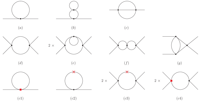
Figure 1: One and two-loop propagator and vertex corrections in the $\lambda\phi^{4}$ theory. Dots represents $\phi^{4}$ vertices, while crosses and squares represent the one-loop propagator and vertex counterterms respectively. Crossing diagrams are not shown.

Let us start by first considering the usual $\lambda\phi^{4}$ theory defined by

$${\cal L}\ =\ \frac{1}{2}(\partial^{\mu}\phi)(\partial_{\mu}\phi)\>-\>\frac{1}{2}m^{2}\phi^{2}\>+\>\frac{\lambda}{4!}\phi^{4}\;.$$ (17)

At the one-loop level, the first equation of (II) gives the usual renormalization prescription in the MS scheme,

$$Z^{(1)}_{\phi} = 2Z^{\frac{1}{2}\,(1)}_{\phi}$$

$$= i\frac{\partial}{\partial p^{2}}\overline{\Gamma_{\phi^{2}}^{(1)}(\lambda_{\mathrm{R}},m_{\mathrm{R}}^{2};\mu,\epsilon)}_{|_{p^{2}=0}}\;,$$

$$Z^{(1)}_{\lambda} = \frac{i}{\lambda_{\mathrm{R}}}\overline{\Gamma_{\phi^{4}}^{(1)}(\lambda_{\mathrm{R}},m_{\mathrm{R}}^{2};\mu,\epsilon)}\;,$$

$$Z^{(1)}_{\phi}+Z^{(1)}_{m^{2}} = -\frac{i}{m_{\mathrm{R}}^{2}}\overline{\Gamma_{\phi^{2}}^{(1)}(\lambda_{\mathrm{R}},m_{\mathrm{R}}^{2};\mu,\epsilon)}_{|_{p^{2}=0}}\;,$$ (18)

where the “bars” indicate that only the infinite part of the corresponding bare Green function should be considered. A straightforward calculation of the one-loop diagrams of Fig. 1 (with $d=4-\epsilon$) gives then

$$Z^{(1)}_{\phi}=0\,,\qquad Z^{(1)}_{m^{2}}=-\frac{1}{(4\pi)^{2}\epsilon}\lambda\,,\qquad Z^{(1)}_{\lambda}=-\frac{1}{(4\pi)^{2}\epsilon}3\lambda\;.$$ (19)

More interesting is the two-loop case, for which the second equation in (II) gives

$$Z^{(2)}_{\phi} = 2Z^{\frac{1}{2}\,(2)}_{\phi}\>+\>\left(Z^{\frac{1}{2}\,(1)}_{\phi}\right)^{2}\$$

$$= i\frac{\partial}{\partial p^{2}}\left[\ \overline{D^{(1)}\Gamma_{\phi^{2}}^{(1)}(\lambda_{\mathrm{R}},m_{\mathrm{R}}^{2};\mu,\epsilon)}+\overline{\Gamma_{\phi^{2}}^{(2)}(\lambda_{\mathrm{R}},m_{\mathrm{R}}^{2};\mu,\epsilon)}\ \right]_{|_{p^{2}=0}},$$

$$Z^{(2)}_{\lambda}+Z^{(2)}_{\phi}+Z^{(1)2}_{\phi}+2Z^{(1)}_{\phi}Z^{(1)}_{\lambda} = \frac{i}{\lambda_{\mathrm{R}}}\left[\ \overline{D^{(1)}\Gamma_{\phi^{4}}^{(1)}(\lambda_{\mathrm{R}},m_{\mathrm{R}}^{2};\mu,\epsilon)}+\overline{\Gamma_{\phi^{4}}^{(2)}(\lambda_{\mathrm{R}},m_{\mathrm{R}}^{2};\mu,\epsilon)}\ \right],$$

$$Z^{(2)}_{m^{2}}+Z^{(2)}_{\phi}+Z^{(1)}_{\phi}Z^{(1)}_{m^{2}} = -\frac{i}{m_{\mathrm{R}}^{2}}\left[\ \overline{D^{(1)}\Gamma_{\phi^{2}}^{(1)}(\lambda_{\mathrm{R}},m_{\mathrm{R}}^{2};\mu,\epsilon)}+\overline{\Gamma_{\phi^{2}}^{(2)}(\lambda_{\mathrm{R}},m_{\mathrm{R}}^{2};\mu,\epsilon)}\ \right]_{|_{p^{2}=0}},$$

where $D^{(1)}$ is now the displacement operator after the one-loop parameters shift has been substituted, i.e.,

$$D^{(1)}\ =\ Z^{(1)}_{\lambda}\lambda_{\mathrm{R}}\frac{\partial}{\partial\lambda_{\mathrm{R}}}\>+\>Z^{(1)}_{m^{2}}m_{\mathrm{R}}^{2}\frac{\partial}{\partial m_{\mathrm{R}}^{2}}\>+\>\frac{n}{2}Z^{(1)}_{\phi}\;,$$ (21)

with $n$ is the number of external $\phi$ legs. Notice that these equations tell us a rather non-trivial fact, i.e., that the combination in square brackets on the right-hand side (RHS) is free of overlapping divergences. This is quite striking, since in the calculation of the two loop Green function $\Gamma_{\phi^{n}}^{(2)}$ only 1PI bare diagrams must be considered (see Fig. 1 again) and no two-loop CT diagram has to be taken into account. Evidently, the $D^{(1)}$ operator, when applied to the lower order (one-loop) $\Gamma^{(1)}_{\phi^{n}}$, will generate the necessary CT at the two-loop order.

Since the $D$ operator and the integration over virtual momenta commute, one has two possibilities: first carry out the integration and then apply $D$, or, vice versa, first apply $D$ and then integrate. These two approaches have both advantages and disantvantages. In the first case, the main advantage is that all explicit references to CTs is removed, and one needs to compute 1PI irreducible diagrams only (no CT diagrams). The disadvantage is related to the fact that, since the $D$ operator involves differentiation with respect to all parameters of the theory that undergo renormalization, we need to maintain the explicit dependence of the various Green functions on them. This is particularly relevant in the case of gauge theories, where one would be faced with the complication of computing diagrams keeping the GFP $\xi$ arbitrary footnote3 . In the second case, instead, one will algebraically generate the CTs and recover the conventional formulation. Of course, after applying the $D$ operator, one can work at a fixed $\xi$ (say, $\xi=1$). To see how the CT diagrams get generated by the displacement operator, observe that the one-loop CT to be added to the Lagrangian are given by

$$\delta c_{1}=\frac{i}{(4\pi)^{2}\epsilon}\lambda m^{2},\qquad\delta c_{2}=-\frac{i}{(4\pi)^{2}\epsilon}3\lambda^{2},$$ (22)

which are related to the renormalization of the operators $\phi^{2}$ and $\phi^{4}$, respectively. Then, by applying the $D$ operator on the bare one-loop 1PI diagrams $(a)$ and $(d)$ of Fig. 1, it is easy to see that

$$D^{(1)}\Gamma_{\phi^{2}}^{(1)} = -i\delta c_{1}\frac{\lambda}{2}\int\!\frac{d^{d}k}{(2\pi)^{d}}\frac{1}{(k^{2}-m^{2})^{2}}+i\delta c_{2}\frac{1}{2}\int\!\frac{d^{d}k}{(2\pi)^{d}}\frac{1}{k^{2}-m^{2}}$$

$$= (c1)+(c2),$$

$$D^{(1)}\Gamma_{\phi^{4}}^{(1)} = 3i\delta c_{1}\lambda^{2}\int\!\frac{d^{d}k}{(2\pi)^{d}}\frac{1}{(k^{2}-m^{2})^{3}}-3i\delta c_{2}\lambda\int\!\frac{d^{d}k}{(2\pi)^{d}}\frac{1}{(k^{2}-m^{2})^{2}}$$ (23)

$$= (c3)+(c4).$$

Therefore, irrespectively of the order, one will get the results

$$Z^{(2)}_{\phi}=-\frac{1}{(4\pi)^{4}}\frac{\lambda^{2}}{12\epsilon},\quad Z^{(2)}_{m^{2}}=-\frac{1}{(4\pi)^{4}}\lambda^{2}\left(\frac{2}{\epsilon^{2}}-\frac{5}{12\epsilon}\right),\quad Z^{(2)}_{\lambda}=-\frac{1}{(4\pi)^{4}}\lambda^{2}\left(\frac{9}{\epsilon^{2}}-\frac{35}{12\epsilon}\right).$$

III.2 Massless QED

We turn to the case of QED, where for simplicity the electron mass is considered to be zero to all orders. In this case the one-loop $D$ operator of the photon vacuum polarization, assumes the form

$$D^{(1)}\ =\ Z^{(1)}_{e}e_{R}\frac{\partial}{\partial e_{R}}+Z^{(1)}_{\xi}\xi_{R}\frac{\partial}{\partial\xi_{R}}+Z^{(1)}_{A}\;,$$ (25)

where $e$ is the QED coupling, and $Z^{(1)}_{e}$, $Z^{(1)}_{A}$ and $Z^{(1)}_{\xi}$ are, respectively, the one loop coupling, wave-function, and GFP renormalization constants. It is then straightforward to establish that the action of the operator $D^{(1)}$ on the one-loop photon vacuum polarization $\Gamma_{A_{\mu}A_{\nu}}^{(1)}$ vanishes. To begin with, the vacuum polarization is independent of the GFP to all orders. In addition, the Abelian gauge symmetry of the theory gives rise to the fundamental Ward identity

$$q^{\mu}\Gamma^{0}_{\mu}(p,p+q)=S_{0}^{-1}(p+q)-S_{0}^{-1}(p)\;,$$ (26)

where $\Gamma^{0}_{\mu}$ and $S_{0}(k)$ are the unrenormalized (all-order) photon-electron vertex (with an $e$ factored out) and electron propagator, respectively. The requirement that the renormalized vertex $\Gamma_{\mu}=Z_{1}\Gamma^{0}_{\mu}$ and the renormalized self-energy $S=Z_{f}^{-1}S_{0}$ satisfy the same identity imposes the equality $Z_{1}=Z_{f}$, from which follows immediately that $Z_{e}=Z_{A}^{-1/2}$, and therefore, after expanding perturbatively, $2Z^{(1)}_{e}+Z^{(1)}_{A}=0$. Then, using that, to the given order,

$$e_{R}\frac{\partial}{\partial e_{R}}\Gamma_{A_{\mu}A_{\nu}}^{(1)}\ =\ 2\Gamma_{A_{\mu}A_{\nu}}^{(1)}\;,$$ (27)

we find immediately that $D^{(1)}\Gamma_{A_{\mu}A_{\nu}}^{(1)}=0$. Evidently, the action of $D^{(1)}$ produces no two-loop CT contributions. This is consistent with the fact that the standard CT graphs (first row in Fig. 2) add up to zero, again by virtue of the aforementioned Ward identity (see for example Itzykson:1980rh ).

At higher orders, the renormalization of the photon vacuum polarization requires CTs that originate from two-loop and higher-order self-energy graphs. Likewise, it is not difficult to show that, on account of the relation $Z_{e}=Z^{-1/2}_{A}$, the CTs from one-loop graphs vanish identically to all orders. In QED with massive quarks and leptons, mass CTs from all lower-order vacuum graphs, including one-loop graphs, contribute to the renormalization of the photon vacuum polarization. In this case, the $D$-formalism is a very practical method to reliably calculate such effects.

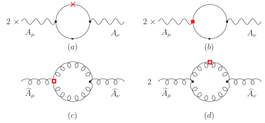
Figure 2: One-loop CTs for massless QED [($a$) and ($b$)], and pure Yang-Mills theory in the background field type of gauges [($c$) and ($d$)]. In the latter case we only draw gauge-fixing term insertions resulting from the renormalization of the GFP.

III.3 Gluon self-energy in the Background Field Method

We next turn to the case of quark-less QCD, formulated in the BFM, and apply the $D$-formalism to study the structure of the two-loop CTs appearing in the calculation of the background gluon self-energy, to be denoted by $\Gamma_{\widehat{A}_{\mu}\widehat{A}_{\nu}}$. The BFM is a special gauge-fixing procedure, which preserves the symmetry of the action under ordinary gauge transformations with respect to the background (classical) gauge field $\widehat{A}^{a}_{\mu}$, while the quantum gauge fields $A^{a}_{\mu}$ appearing in the loops transform homogeneously under the gauge group Weinberg:kr . As a result, the $n$-point functions $\langle 0|T\left[\widehat{A}^{a_{1}}_{\mu_{1}}(x_{1})\widehat{A}^{a_{2}}_{\mu_{2}}(x_{2})\dots\widehat{A}^{a_{n}}_{\mu_{n}}(x_{n})\right]|0\rangle$ satisfy naive, QED-like Ward identities, instead of the Slavnov–Taylor identities valid in the usual covariant quantization. Notice also that the $n$-point functions depend explicitly on the quantum GFP $\xi_{Q}$.

In this case, the one-loop $D$ operator for the (background) gluon vacuum polarization is given by

$$D^{(1)}\ =\ Z^{(1)}_{g}g_{R}\frac{\partial}{\partial g_{R}}\>+\>Z^{(1)}_{\xi_{Q}}\xi_{Q}\frac{\partial}{\partial\xi_{Q}}\>+\>Z^{(1)}_{\widehat{A}}\;,$$ (28)

Here and in the following, $\xi_{Q}$ stands for the renormalized GFP associated with the quantum gauge field $A^{a}_{\mu}(x)$. Because of the aforementioned background gauge symmetry, $Z_{g}$ and $Z_{\widehat{A}}$ satisfy to all orders the QED-like relation $Z_{g}\ =\ Z_{\widehat{A}}^{-1/2}$, from which follows that the first and third term of $D^{(1)}$ cancel against each other, as happens for the photon vacuum polarization. Therefore, $D^{(1)}$ reduces to

$$D^{(1)}\ =\ Z^{(1)}_{\xi_{Q}}\xi_{Q}\frac{\partial}{\partial\xi_{Q}}.$$ (29)

On the other hand notice that, contrary to the case of the photon vacuum polarization, the background gluon self-energy $\Gamma_{\widehat{A}_{\mu}\widehat{A}_{\nu}}$ depends explicitly on $\xi_{Q}$. This dependence stems not only from the tree-level (quantum) gluon propagator appearing in the loop,

$$\Delta_{\mu\nu}^{[0]}(k)\ =\ -\frac{i}{k^{2}}\left[\ g_{\mu\nu}-(1-\xi_{Q})\frac{k_{\mu}k_{\nu}}{k^{2}}\right],$$ (30)

as happens in the case of the covariant gauges, but in addition from the tree-level vertices between a background gluon $\widehat{A}^{a}_{\mu}(p)$ and two quantum gluons $A^{b}_{\nu}(q)$ and $A^{c}_{\lambda}(k)$,

$$\Gamma^{abc}_{\mu\nu\rho}(p,q,k)\ =\ gf^{abc}\left[g_{\mu\rho}\left(p-k-\xi_{Q}^{-1}q\right)_{\nu}+g_{\nu\rho}\left(k-q\right)_{\mu}+g_{\mu\nu}\left(q-p+\xi_{Q}^{-1}k\right)_{\rho}\right]\;,$$ (31)

which, unlike the usual case, also depend on $\xi_{Q}$. Finally, as a consequence of the non-renormalization of the longitudinal part of the gluon self-energy to all orders, we know that $Z_{\xi_{Q}}=Z_{A}$ Capper:1982tf , where $Z_{A}$ is the wave-function renormalization of the quantum gluons; it coincides with the one computed in the covariant gauges. Thus, at one-loop (recall that in our conventions $d=4-\epsilon$)

$$Z_{\xi_{Q}}^{(1)}\ =\ \frac{g^{2}C_{A}}{(4\pi)^{2}}\left(\frac{13}{3}-\xi_{Q}\right)\frac{1}{\epsilon}\;.$$ (32)

Therefore the action of $D^{(1)}$ will be non-trivial, and will generate automatically all necessary two-loop CTs (Fig. 2 second row). Notice that this is in complete accordance with the fact that the only CTs appearing in the classic two-loop calculation of Abbott:1980hw are precisely related to the gauge-fixing. The advantage of the $D$-formalism in this respect is that the presence of such CTs does not have to be deduced, but is given directly from the very form of the $D$ operator.

In order to verify that the action of $D^{(1)}$ on $\Gamma_{\widehat{A}_{\mu}\widehat{A}_{\nu}}^{(1)}$ generates indeed the two-loop CT contributions, one may follow two equivalent ways. First, one may differentiate directly on the Feynman diagram determining $\Gamma_{\widehat{A}_{\mu}\widehat{A}_{\nu}}^{(1)}$, taking into account the dependence of the propagators and vertices on $\xi_{Q}$, as shown above, and setting eventually $\xi_{Q}=1$. Thus, one generates immediately the Feynman graphs appearing in the second row of Fig. 2.

The second, more algebraic way, is to actually act with the $D^{(1)}$ of (29) on the expression that one obtains for $\Gamma_{\widehat{A}_{\mu}\widehat{A}_{\nu}}^{(1)}$ after the loop integration, and verify that it is actually equal to the sum of the CT diagrams, whose individual expressions, calculated at $\xi_{Q}=1$, are listed in the Table 1 of Abbott:1980hw [where the two diagrams ($c$) and ($d$) are called ($l$) and ($m$) respectively]. The latter sum reads

$$(c)+(d)\ =\ \frac{g^{4}C_{A}^{2}}{(4\pi)^{4}}\delta^{ab}\Bigg{(}q^{2}g_{\mu\nu}-q_{\mu}q_{\nu}\Bigg{)}\frac{20}{3}\frac{1}{\epsilon}\ .$$ (33)

In doing so, note that, as is well known, the $\xi_{Q}$-dependent part, $\tilde{\Gamma}_{\widehat{A}_{\mu}\widehat{A}_{\nu}}^{(1)}$, is finite, and is given by Papavassiliou:1994yi

$$\tilde{\Gamma}_{\widehat{A}_{\mu}^{a}\widehat{A}_{\nu}^{b}}^{(1)}(q)\ =\ \frac{g^{2}C_{A}}{(4\pi)^{2}}\delta^{ab}\Bigg{(}q^{2}g_{\mu\nu}-q_{\mu}q_{\nu}\Bigg{)}\frac{(\xi_{Q}-1)(7+\xi_{Q})}{4}\ .$$ (34)

At this point, acting with $D^{(1)}$ on $\tilde{\Gamma}_{\widehat{A}_{\mu}\widehat{A}_{\nu}}^{(1)}$ of (34), and setting afterwards $\xi_{Q}=1$, we immediately recover the result of (33), as announced.

IV Deformations of the Nielsen Identities

One of the main advantages of the $D$-formalism is that it allows to obtain complete control over the deformations, caused by renormalization, on the NI, which describe the GFP dependence of the bare Green functions.

To be specific, let us consider the Abelian Higgs-Kibble model in the symmetric phase, described by the Lagrangian (see also Appendix A)

$${\cal L}\ =\ {\cal L}_{\rm I}\>+\>{\cal L}_{\rm GF}\>+\>{\cal L}_{\rm FP}\;.$$ (35)

Here, ${\cal L}_{\rm I}$ is the $U(1)$ invariant term

$${\cal L}_{\rm I}\ =\ -\frac{1}{4}F^{\mu\nu}F_{\mu\nu}+\left(D_{\mu}\Phi\right)^{*}\left(D^{\mu}\Phi\right)-m^{2}\Phi^{*}\Phi-\lambda\left(\Phi^{*}\Phi\right)^{2},$$ (36)

with

$$F_{\mu\nu}=\partial_{\mu}A_{\nu}-\partial_{\nu}A_{\mu}\;,\qquad D_{\mu}=\partial_{\mu}-igYA_{\mu}\;,\qquad\Phi=\frac{1}{\sqrt{2}}(H+iG)\;,$$ (37)

and the hypercharge assignment $Y_{\Phi}=1$. The generic gauge-fixing and Faddeev-Popov ghost terms are given by

$${\cal L}_{\rm GF} = \frac{\xi}{2}B^{2}+BF\;,$$

$${\cal L}_{\rm FP} = -\bar{c}(sF)\;,$$ (38)

where $B$ is an auxiliary non propagating field (which can be eliminated through its equations of motion), $F$ is the gauge-fixing function, and $s$ is the BRS operator, giving rise to the following field transformations

$$sA_{\mu}=\partial_{\mu}c,\qquad sH=-gcG, \qquad sG=gcH,$$

$$sc=0,\qquad s\bar{c}=B, \qquad sB=0,$$ (39)

with $s$ nilpotent. Evidently, ${\cal L}$ is BRS invariant.

Let us now promote the constant $\xi$ to a (static) field, and introduce an associate anticommuting BRS source $\eta$ (with $\eta^{2}=0$) footnote4 through the transformations

$$s\xi=\eta\,,\qquad s\eta=0\;.$$ (40)

The BRS invariance of the original Lagrangian ${\cal L}$ is then lost, unless we add to it the term

$${\cal L}_{\rm N}\ =\ \frac{1}{2}\eta\bar{c}B\;,$$ (41)

which couples the $\eta$ source to the other fields. With the Lagrangian term ${\cal L}_{\rm N}$ included, it can be easily checked that the so-quantized Lagrangian,

$${\cal L}\ =\ {\cal L}_{\rm I}\>+\>{\cal L}_{\rm GF}\>+\>{\cal L}_{\rm FP}\>+\>{\cal L}_{\rm N}\;,$$ (42)

is invariant under the extended BRS ($e$BRS) transformations given by (39) and (40). If we integrate out the auxiliary field $B$, we find

$$B=-\frac{1}{\xi}F-\frac{1}{2}\eta\bar{c},\qquad{\cal L}_{\rm GF}=-\frac{1}{2\xi}F^{2},\qquad{\cal L}_{\rm N}=-\frac{1}{2\xi}\eta\bar{c}F.$$ (43)

In this case, however, the $e$BRS transformation of the antighost $\bar{c}$ is not nilpotent, because one has

$$s^{2}\bar{c}\ =\ \frac{1}{\xi}\left(-sF+\frac{1}{2\xi}\eta F\right),$$ (44)

where the term in parenthesis is precisely the antighost field equation of motion. Hence, in this case, the $e$BRS algebra closes on-shell.

The extended Slavnov–Taylor identities one obtains from the $e$BRS invariant Lagrangian are precisely the NI. Specifically, assuming that the $B$ field has been integrated out, the generating functional for connected Green functions of our model can be written as

$$e^{iZ} = \int\![dA_{\mu}][dc][d\bar{c}][dH][dG]\,\exp\bigg{\{}i\int\!d^{4}x\,\Big{[}{\cal L}+J_{A}^{\mu}A_{\mu}+J_{c}c+J_{\bar{c}}\bar{c}+J_{H}H+J_{G}G$$ (45)

$$+K_{H}(sH)+K_{G}(sG)+K_{\bar{c}}(s\bar{c})\Big{]}\bigg{\}}\,,$$

where the $e$BRS sources $K$ (sometimes called the antifields) have been included only for fields transforming non linearly under the algebra of (39) and (40). Notice that the antighost source $K_{\bar{c}}$ must be included, since the $B$ field has been integrated out [and therefore $\bar{c}$ transforms non-linearly under $e$BRS, see (43)]. Observe that, given a field $\Phi$, its corresponding BRS source $K_{\Phi}$ obeys opposite statistic, and has ghost charge $Q_{\mathrm{FP}}(K_{\Phi})=-Q_{\mathrm{FP}}(\Phi)-1$; therefore one has $Q_{\mathrm{FP}}(K_{A_{\mu}},K_{H},K_{G},K_{\bar{c}})=\{-1,-1,-1,0\}$ (that $K_{\bar{c}}$ has no ghost charge is evident from the fact that it couples to $s\bar{c}=B$ and the action must have zero ghost charge).

Thus, eventually the statement of $e$BRS invariance implies the following Slavnov–Taylor identity:

$$Z[J_{A}^{\mu},J_{c},J_{\bar{c}},J_{H},J_{G},K_{\bar{c}},K_{H},K_{G};\xi,\eta]$$ (46)

$$=\ Z[J_{A}^{\mu},J_{c}-\omega\partial_{\mu}J_{A}^{\mu},J_{\bar{c}},J_{H},J_{G},K_{\bar{c}}+\omega J_{\bar{c}},K_{H}+\omega J_{H},K_{G}+\omega J_{G};\xi-\omega\eta,\eta]\;,\qquad$$

which, after a Taylor expansion in $\omega$ (with $\omega^{2}=0$), reduces to the (all-order) NI

$$J_{A}^{\mu}\partial_{\mu}\frac{\delta Z}{\delta J_{c}}+J_{\bar{c}}\frac{\delta Z}{\delta K_{\bar{c}}}+J_{H}\frac{\delta Z}{\delta K_{H}}+J_{G}\frac{\delta Z}{\delta K_{G}}-\eta\partial_{\xi}Z\ =\ 0\;.$$ (47)

Denoting by $\varphi$ all the fields of our model, i.e., $\varphi=\{A_{\mu},c,\bar{c},H,G\}$, one can express the previous Slavnov–Taylor identities in terms of the effective action ${\rm I}\Gamma[\varphi_{\rm cl},K_{\varphi};\xi,\eta]$, given by the Legendre transform

$${\rm I}\Gamma[\varphi_{\rm cl},K_{\varphi};\xi,\eta]\ =\ Z[J_{\varphi},K_{\varphi};\xi,\eta]\>-\>\int d^{4}xJ_{\varphi}\varphi_{\rm cl}\;,$$ (48)

with $\varphi_{\rm cl}=\delta Z/\delta J_{\varphi}$. Taking into account the relations

$$\frac{\delta{\rm I}\Gamma}{\delta\varphi_{\rm cl}}=-J_{\varphi}\,,\qquad\frac{\delta{\rm I}\Gamma}{\delta K_{\varphi}}=\frac{\delta Z}{\delta K_{\varphi}}\ ,\qquad\partial_{\xi}{\rm I}\Gamma=\partial_{\xi}Z\;,$$ (49)

we obtain

$$\frac{\delta{\rm I}\Gamma}{\delta A^{\mu}_{\rm cl}}\partial_{\mu}c_{\rm cl}+\frac{\delta{\rm I}\Gamma}{\delta\bar{c}_{\rm cl}}\frac{\delta{\rm I}\Gamma}{\delta K_{\bar{c}}}+\frac{\delta{\rm I}\Gamma}{\delta H_{\rm cl}}\frac{\delta{\rm I}\Gamma}{\delta K_{H}}+\frac{\delta{\rm I}\Gamma}{\delta G_{\rm cl}}\frac{\delta{\rm I}\Gamma}{\delta K_{G}}+\eta\partial_{\xi}{\rm I}\Gamma\ =\ 0\;.$$ (50)

Finally, after differentiating with respect to $\eta$ and setting $\eta$ afterwards to zero (with $\eta^{2}=0$), we obtain the NI in its final form

$$\partial_{\xi}{\rm I}\Gamma\Big{|}_{\eta=0}\ =\ -\,\partial_{\eta}\left(\,\frac{\delta{\rm I}\Gamma}{\delta A^{\mu}_{\rm cl}}\partial_{\mu}c_{\rm cl}\>+\>\frac{\delta{\rm I}\Gamma}{\delta\bar{c}_{\rm cl}}\frac{\delta{\rm I}\Gamma}{\delta K_{\bar{c}}}\>+\>\frac{\delta{\rm I}\Gamma}{\delta H_{\rm cl}}\frac{\delta{\rm I}\Gamma}{\delta K_{H}}\>+\>\frac{\delta{\rm I}\Gamma}{\delta G_{\rm cl}}\frac{\delta{\rm I}\Gamma}{\delta K_{G}}\,\right)\;.$$ (51)

Introducing the so-called Slavnov–Taylor operator ${\cal S}_{{\rm I}\Gamma}$, the NI (51) is often written down as

$$\partial_{\xi}{\rm I}\Gamma\Big{|}_{\eta=0}\ =\ {\cal S}_{{\rm I}\Gamma}\,\Big{[}\,\partial_{\eta}{\rm I}\Gamma\,\Big{]}\;,$$ (52)

where we have used that $[{\cal S}_{{\rm I}\Gamma}\,,\,\partial_{\eta}]=0$. It is now easy to see that, due to ghost charge conservation, the first term on the RHS of (51) becomes relevant only when one is calculating the gauge-dependence of ghost Green functions. For instance, it contributes a term $-\partial_{\mu}\Gamma_{\bar{c}\eta A_{\mu}}$ for the NI of the ghost self-energy $\Gamma_{c\bar{c}}$.

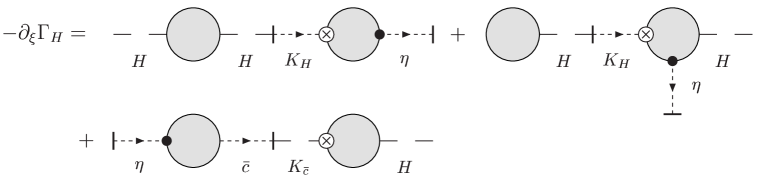
Figure 3: Graphic representation of the NI (in this case the one for the tadpole). Notice that the arrows indicate the flow of the ghost charge. The last term is absent to all orders in the $R_{\xi}$ gauge.

A graphical representation of the NI can be obtained as follows. The $\eta$ coupling can be represented by a heavy dot attached to a dotted line with an arrow that indicates the flow of the ghost charge. Likewise, the coupling of the BRS sources $K_{H}$ and $K_{G}$ should by represented by a $\otimes$ symbol attached to an arrowed dotted line. On the other hand, the coupling of $K_{\bar{c}}$ should be represented by $\otimes$ attached to a dashed line without an arrow, since $K_{\bar{c}}$ has no ghost charge. In this way, a consistent graphical picture conveying information of the flow of the ghost charge emerges. For example, the NI for the Higgs tadpole, that reads (assuming $CP$ conservation)

$$-\partial_{\xi}\Gamma_{H}\ \equiv\ -{\cal S}_{{\rm I}\Gamma}\Big{[}\,\partial_{\eta}\Gamma_{H}\,\Big{]}\ =\ \Gamma_{HH}\Gamma_{\eta K_{H}}+\Gamma_{H}\Gamma_{\eta K_{H}H}+\Gamma_{\eta\bar{c}}\Gamma_{K_{\bar{c}}H}\;,$$ (53)

can be represented as in Fig. 3. It can be explicitly checked that the last term on the RHS of (53) is zero to all orders in perturbation theory in the conventional $R_{\xi}$ gauge-fixing scheme.

As already mentioned in the Introduction, unlike the Slavnov–Taylor identities which are derived from the BRS invariance of the theory, the NI are obtained from the $e$BRS symmetry; therefore they will not remain unmodified by the process of renormalization, but they will be deformed. In what follows, we are going to determine a closed expression for the deformation of the NI under renormalization, by applying the $D$-formalism.

Let us therefore denote by $x$ the parameters of the theory (coupling, masses, etc.) except of the GFP $\xi$, and with $\phi_{i}$ the fields $A_{\mu},H,$ and $G$, with renormalization relations given by (12). To elucidate our points, we will initially consider Green functions involving $n$ fields of one type, say $\phi$, and then we will generalize our results to Green functions involving different types of fields. Based on the basic formulæ (6) and (7) of the $D$-formalism, we can now study the response of the renormalized Green functions to a variation $\Delta\xi_{\mathrm{R}}$ of the renormalized GFP $\xi_{\mathrm{R}}$, i.e.,

$$\phi^{n}_{\mathrm{R}}\Gamma^{\mathrm{R}}_{\phi^{n}}(x_{\mathrm{R}},\xi_{\mathrm{R}}+\Delta\xi_{\mathrm{R}};\mu)-\phi^{n}_{\mathrm{R}}\Gamma^{\mathrm{R}}_{\phi^{n}}(x_{\mathrm{R}},\xi_{\mathrm{R}};\mu)\ =\ \phi^{n}_{\mathrm{R}}\Delta\xi_{\mathrm{R}}\partial_{\xi_{\mathrm{R}}}\Gamma^{\mathrm{R}}_{\phi^{n}}(x_{\mathrm{R}},\xi_{\mathrm{R}};\mu)\ +\ {\cal{O}}(\Delta\xi_{\mathrm{R}}^{2})\,.$$ (54)

In stating (54), we have assumed that the renormalized fields and parameters $\phi_{\rm R}$ and $x_{\rm R}$ are GFP-independent in a given renormalization scheme R. In fact, this is the case, if the renormalized parameters are evaluated from renormalization conditions that are manifestly GFP independent, e.g., from physical observables, such as $S$-matrix elements, or from gauge-invariant operators, within a good regularization scheme that preserves the Slavnov–Taylor identities. In general, the GFP independence of the renormalized parameters in a specific scheme can be determined in two ways: (i) by showing that the corresponding CTs are GFP-independent; (ii) by comparing it to another gauge-invariant scheme, such as the $\overline{\rm MS}$ MSbar or the pole-mass scheme Stuart:1991xk ; Sirlin:1991fd . An exception to the above are the renormalized field $\phi_{\rm R}$ and its VEV $v_{\rm R}$. These parameters are GFP-independent, but their respective renormalizations $Z_{\phi}^{\frac{1}{2}}$ and $Z_{v}$ are in general GFP-dependent, even within the $\overline{\rm MS}$ scheme. Thus, although we will initially assume that $\phi_{\rm R}$ and $x_{\rm R}$ are GFP-independent, we will also comment on the modifications that should be considered, if $x_{\rm R}$ were depending on $\xi_{\rm R}$.

Let us concentrate on the LHS of (54), and more precisely on its first term. From (1), we will have that

$$\phi^{n}_{\mathrm{R}}\Gamma^{\mathrm{R}}_{\phi^{n}}(x_{\mathrm{R}},\xi_{\mathrm{R}}+\Delta\xi_{\mathrm{R}};\mu) = \Big{(}\phi_{\mathrm{R}}+\delta\phi(\xi_{\mathrm{R}}+\Delta\xi_{\mathrm{R}})\Big{)}^{n}$$ (55)

$$\times\,\Gamma_{\phi^{n}}\Big{(}x_{\mathrm{R}}+\delta x(\xi_{\mathrm{R}}+\Delta\xi_{\mathrm{R}}),\xi_{\mathrm{R}}+\Delta\xi_{\mathrm{R}}+\delta\xi(\xi_{\mathrm{R}}+\Delta\xi_{\mathrm{R}});\mu,\epsilon\Big{)}$$

$$= \Big{(}\phi_{\mathrm{R}}+\delta\phi(\xi_{\mathrm{R}})\Big{)}^{n}\;\Gamma_{\phi^{n}}\Big{(}x_{\mathrm{R}}+\delta x(\xi_{\mathrm{R}}),\xi_{\mathrm{R}}+\delta\xi(\xi_{\mathrm{R}});\mu,\epsilon\Big{)}$$

$$+\,\Delta\xi_{\mathrm{R}}\Big{(}\phi_{\mathrm{R}}+\delta\phi(\xi_{\mathrm{R}})\Big{)}^{n}\Big{[}\,n\Big{(}\phi_{\mathrm{R}}+\delta\phi(\xi_{\mathrm{R}})\Big{)}^{-1}\Big{(}\partial_{\xi_{\mathrm{R}}}\delta\phi(\xi_{\mathrm{R}})\Big{)}$$

$$+\,\Big{(}\partial_{\xi_{\mathrm{R}}}\delta x(\xi_{\mathrm{R}})\Big{)}\partial_{x_{\mathrm{R}}+\delta x}\>+\>\Big{(}1+\partial_{\xi_{\mathrm{R}}}\delta\xi(\xi_{\mathrm{R}})\Big{)}\partial_{\xi_{\mathrm{R}}+\delta\xi}\Big{]}$$

$$\times\,\Gamma_{\phi^{n}}\Big{(}x_{\mathrm{R}}+\delta x(\xi_{\mathrm{R}}),\xi_{\mathrm{R}}+\delta\xi(\xi_{\mathrm{R}});\mu,\epsilon\Big{)}\ +\ {\cal{O}}(\Delta\xi_{\mathrm{R}}^{2})\;.$$

Substituting for the shifts their expressions in terms of renormalization constants [cf. (14)], and then inserting the result back into (55), we obtain for the RHS of (54) that

$$\phi^{n}_{\mathrm{R}}\partial_{\xi_{\mathrm{R}}}\Gamma^{\mathrm{R}}_{\phi^{n}}(x_{\mathrm{R}},\xi_{\mathrm{R}};\mu)\! = \!\phi^{n}\,\Big{[}\partial_{\xi_{\mathrm{R}}}(Z_{\xi}\xi_{\mathrm{R}})\Big{]}\,\partial_{\xi}\Gamma_{\phi^{n}}(x,\xi;\mu,\epsilon)\,+\,Z_{\phi}^{\frac{n}{2}}\phi^{n}_{\mathrm{R}}\Big{(}\partial_{\xi_{\mathrm{R}}}Z_{x}\Big{)}\,x_{\rm R}\,\partial_{x}\Gamma_{\phi^{n}}(x,\xi;\mu,\epsilon)$$ (56)

$$+\,n\phi^{n}_{\mathrm{R}}\,\Big{(}\partial_{\xi_{\mathrm{R}}}\ln Z_{\phi}^{\frac{1}{2}}\Big{)}\,\Gamma^{\mathrm{R}}_{\phi^{n}}(x_{\mathrm{R}},\xi_{\mathrm{R}};\mu)\;,$$

which is equivalent to the identity

$$\partial_{\xi_{\mathrm{R}}}\Gamma^{\mathrm{R}}_{\phi^{n}}(x_{\mathrm{R}},\xi_{\mathrm{R}};\mu) = Z_{\phi}^{\frac{n}{2}}\Big{[}\partial_{\xi_{\mathrm{R}}}(Z_{\xi}\xi_{\mathrm{R}})\Big{]}\partial_{\xi}\Gamma_{\phi^{n}}(x,\xi;\mu,\epsilon)\,+\,Z_{\phi}^{\frac{n}{2}}\Big{(}\partial_{\xi_{\mathrm{R}}}Z_{x}\Big{)}x_{\rm R}\partial_{x}\Gamma_{\phi^{n}}(x,\xi;\mu,\epsilon)$$ (57)

$$+\,n\,\Big{(}\partial_{\xi_{\mathrm{R}}}\ln Z_{\phi}^{\frac{1}{2}}\Big{)}\,\Gamma^{\mathrm{R}}_{\phi^{n}}(x_{\mathrm{R}},\xi_{\mathrm{R}};\mu)\;.$$

Finally, including $\xi$ in the parameters $x$, we may cast (57) into the slightly more compact form:

$$\partial_{\xi_{\mathrm{R}}}\Gamma^{\mathrm{R}}_{\phi^{n}}(x_{\mathrm{R}};\mu) = Z_{\phi}^{\frac{n}{2}}Z_{\xi}\partial_{\xi}\Gamma_{\phi^{n}}(x;\mu,\epsilon)\>+\>Z_{\phi}^{\frac{n}{2}}\,\Big{(}\partial_{\xi_{\mathrm{R}}}Z_{x}\Big{)}\,x_{\rm R}\,\partial_{x}\Gamma_{\phi^{n}}(x;\mu,\epsilon)$$ (58)

$$+\,n\,\Big{(}\partial_{\xi_{\mathrm{R}}}\ln Z_{\phi}^{\frac{1}{2}}\Big{)}\,\Gamma^{\mathrm{R}}_{\phi^{n}}(x_{\mathrm{R}};\mu)\;.$$

A similar line of arguments can be followed, if $x_{\rm R}$ depends on $\xi_{\rm R}$. In this case, the factor $(\partial_{\xi_{\mathrm{R}}}Z_{x})x_{\rm R}$ contained in the second term on the RHS of (58) should be replaced with $\partial_{\xi_{\mathrm{R}}}(Z_{x}x_{\rm R})$, for $x_{\rm R}\neq\xi_{\rm R}$.

We may now rely on the $D$-formalism to express the RHS of (58) entirely in terms of renormalized parameters. In this way, we obtain the deformed NI

$$\partial_{\xi_{\mathrm{R}}}\Gamma^{\mathrm{R}}_{\phi^{n}}(x_{\mathrm{R}};\mu) = Z_{\phi}^{\frac{n}{2}}Z_{\xi}\>\Big{<}\,e^{D}\,{\cal S}_{{\rm I}\Gamma}\Big{[}\,\partial_{\eta}\Gamma_{\phi^{n}}(x_{\rm R};\mu,\eta,\epsilon)\,\Big{]}\,\Big{>}$$

$$+\,Z_{\phi}^{\frac{n}{2}}\,\Big{(}\partial_{\xi_{\mathrm{R}}}Z_{x}\Big{)}\,x_{\rm R}\,\>\Big{<}\,e^{D}\,\partial_{x_{\rm R}}\Gamma_{\phi^{n}}(x_{\rm R};\mu,\epsilon)\,\Big{>}\>+\>n\,\Big{(}\partial_{\xi_{\mathrm{R}}}\ln Z_{\phi}^{\frac{1}{2}}\Big{)}\,\Gamma^{\mathrm{R}}_{\phi^{n}}(x_{\mathrm{R}};\mu)\;.$$

Notice that, up to an overall constant, only the first term on the RHS of (IV) can be related to the undeformed, unrenormalized NI (52), where the 1PI Green functions involved are evaluated with renormalized parameters. The appearance of the other terms is a consequence of the renormalization process. We emphasize that, unlike earlier formal treatments Gambino:1999ai , Equation (IV) furnishes for the first time the precise closed and, in principle, calculable expression for the deformations of the NI.

It is interesting to remark that even the action of the operator $e^{D}$ present in the first term on the RHS of (IV) gives rise to further deformations. To make this last point more explicit, we first observe that the action of the $D$ operator in (IV) is actually equivalent to the action of a reduced operator $\widetilde{D}$, without the field derivatives, i.e., $\widetilde{D}=D-\sum_{i}\delta\phi_{i}\,\partial/\partial\phi_{i{\rm R}}$. Making use of this last observation, we decompose $e^{D}$, or equivalently $e^{\widetilde{D}}$, as $e^{\widetilde{D}}=1+(e^{\widetilde{D}}-1)$. Subsequently, noticing that the operators $\widetilde{D}$ and ${\cal S}_{{\rm I}\Gamma}$ commute, i.e., $[\widetilde{D}\,,{\cal S}_{{\rm I}\Gamma}]=0$, the first term on the RHS of (IV) can be rewritten, up to the multiplicative factors $Z_{\phi}^{\frac{n}{2}}Z_{\xi}$, as

$$\Big{<}\,e^{D}\,{\cal S}_{{\rm I}\Gamma}\Big{[}\,\partial_{\eta}\Gamma_{\phi^{n}}(x_{\rm R};\mu,\eta,\epsilon)\,\Big{]}\,\Big{>} = \Big{<}\,{\cal S}_{{\rm I}\Gamma}\Big{[}\,\partial_{\eta}\Gamma_{\phi^{n}}(x_{\rm R};\mu,\eta,\epsilon)\,\Big{]}\,\Big{>}$$ (60)

$$+\>\Big{<}\,{\cal S}_{{\rm I}\Gamma}\Big{[}\,(e^{\widetilde{D}}-1)\,\partial_{\eta}\Gamma_{\phi^{n}}(x_{\rm R};\mu,\eta,\epsilon)\,\Big{]}\,\Big{>}\;.$$

Thus, only the first term can be expressed in terms of the undeformed, unrenormalized NI of (52), whereas the second one is an additive deformation of the NI that results in from a BRS variation of another function Gambino:1999ai .

The generalization of (IV) to Green functions involving different types of fields is straightforward footnote5 , and reads

$$\partial_{\xi_{\mathrm{R}}}\Gamma^{\mathrm{R}}_{\prod_{i}\phi^{n_{i}}_{i}}(x_{\mathrm{R}};\mu) = \prod_{i}Z_{\phi_{i}}^{\frac{n_{i}}{2}}Z_{\xi}\,\Big{<}\,e^{D}\,{\cal S}_{{\rm I}\Gamma}\Big{[}\,\partial_{\eta}\,\Gamma_{\prod_{i}\phi^{n_{i}}_{i}}(x_{\rm R};\mu,\eta,\epsilon)\,\Big{]}\,\Big{>}$$

$$+\>\prod_{i}Z_{\phi_{i}}^{\frac{n_{i}}{2}}\sum_{x}\Big{(}\partial_{\xi_{\mathrm{R}}}Z_{x}\Big{)}\,x_{\rm R}\>\Big{<}\,e^{D}\,\partial_{x_{\rm R}}\Gamma_{\prod_{i}\phi^{n_{i}}_{i}}(x_{\rm R};\mu,\epsilon)\,\Big{>}$$

$$+\>\sum_{i}n_{i}\Big{(}\partial_{\xi_{\mathrm{R}}}\ln Z_{\phi_{i}}^{\frac{1}{2}}\Big{)}\Gamma^{\mathrm{R}}_{\prod_{i}\phi^{n_{i}}_{i}}(x_{\mathrm{R}};\mu)\;.$$

In order to get a feel on the structure of Equation (IV), let us apply it to the lowest non-trivial order. Expanding consistently, according to the $D$-formalism, we obtain the following one-loop result:

$$\partial_{\xi_{\mathrm{R}}}\Gamma^{\mathrm{R}\,(1)}_{\prod_{i}\phi^{n_{i}}_{i}}(x_{\mathrm{R}};\mu) = \partial_{\xi_{\mathrm{R}}}\Gamma^{(1)}_{\prod_{i}\phi^{n_{i}}_{i}}(x_{\rm R};\mu,\epsilon)+\sum_{i}\frac{n_{i}}{2}\left(\partial_{\xi_{\mathrm{R}}}Z^{(1)}_{\phi_{i}}\right)\Gamma^{\mathrm{R}\,(0)}_{\prod_{i}\phi^{n_{i}}_{i}}(x_{\mathrm{R}})$$ (62)

$$+\Big{(}\sum_{i}\frac{n_{i}}{2}Z^{(1)}_{\phi_{i}}+Z^{(1)}_{\xi}+\sum_{x}Z^{(1)}_{x}x_{\rm R}\partial_{x_{\rm R}}\Big{)}\partial_{\xi_{\mathrm{R}}}\Gamma^{(0)}_{\prod_{i}\phi^{n_{i}}_{i}}(x_{\rm R})$$

$$+\sum_{x}\left(\partial_{\xi_{\mathrm{R}}}Z^{(1)}_{x}\right)x_{\rm R}\partial_{x_{\rm R}}\Gamma^{(0)}_{\prod_{i}\phi^{n_{i}}_{i}}(x_{\rm R})\;,$$

where the first term is the one-loop NI of (51), with the simple replacement of bare parameters by renormalized ones.

A further simplification of the formulae above occurs in a gauge-invariant renormalization scheme, such as the $\overline{\mathrm{MS}}$ scheme. In this case, all terms proportional to $\partial_{\xi_{\mathrm{R}}}Z_{x}$, for which $x$ is related to a gauge-invariant operator (e.g., a gauge-coupling constant or a gauge-invariant mass parameter), will drop out from the RHS of (IV), as their multiplicative renormalization constants will be $\xi_{\rm R}$-independent.

V The Abelian Higgs model in the HLET-preserving gauges

In this section we will discuss the Abelian Higgs model quantized in the type of gauges that preserve the Higgs-boson Low Energy Theorem (HLET). The Lagrangian defining the model is given by

$${\cal L}\ =\ {\cal L}_{\rm I}\>+\>{\cal L}_{\rm GF}\>+\>{\cal L}_{\rm FP}\;.$$ (63)

Here ${\cal L}_{\rm I}$ is the gauge-invariant part of the Lagrangian

$${\cal L}_{\rm I} = -\frac{1}{4}F^{\mu\nu}F_{\mu\nu}+\left(D_{\mu}\Phi\right)^{*}\left(D^{\mu}\Phi\right)-m^{2}\Phi^{*}\Phi-\lambda\left(\Phi^{*}\Phi\right)^{2}$$ (64)

$$+\,\sum_{i}\bar{f}_{i}^{L}(i\gamma^{\mu}D_{\mu})f_{i}^{L}+\sum_{i}\bar{f}^{R}_{i}(i\gamma^{\mu}\partial_{\mu})f^{R}_{i}$$

$$-\,\sqrt{2}h_{1}\bar{f}^{L}_{1}\Phi f^{R}_{1}-\sqrt{2}h_{2}\bar{f}^{L}_{2}\Phi^{*}f^{R}_{2}-\sqrt{2}h_{1}\bar{f}^{R}_{1}\Phi^{*}f^{L}_{1}-\sqrt{2}h_{2}\bar{f}^{R}_{2}\Phi f^{L}_{2}\ .$$

In (64), $F_{\mu\nu}=\partial_{\mu}A_{\nu}-\partial_{\nu}A_{\mu}$ is the $U(1)_{Y}$ Field strength tensor, $D_{\mu}=\partial_{\mu}-igYA_{\mu}$ is the corresponding covariant derivative, and

$$\Phi\ =\ \frac{1}{\sqrt{2}}\;\Big{(}\,v\,+\,H\,+\,iG\Big{)}$$ (65)

is the complex Abelian Higgs field, composed from the two real fields $H$ and $G$, where $\langle\Phi\rangle=v/\sqrt{2}$ is its VEV that signifies the spontaneous symmetry breaking of $U(1)_{Y}$. The hypercharge quantum numbers of the different fields are assigned according to $Y_{\Phi}=1$, $Y_{1}^{L}=-Y_{2}^{L}=1$, and $Y_{1}^{R}=Y_{2}^{R}=0$. For simplicity, we finally assume that the Yukawa couplings $h_{i}$ are real.

For the gauge-fixing term ${\cal L}_{\rm GF}$ in (63), we will adopt the one introduced in Kastening:1993zn ; Pilaftsis:1997fe , i.e.,

$${\cal L}_{\rm GF} = -\frac{\sigma}{2\xi}[\partial_{\mu}A^{\mu}+\xi g\,{\rm Im}(\Phi^{2})]^{2}$$ (66)

$$= -\frac{\sigma}{2\xi}\Big{[}\partial_{\mu}A^{\mu}\>+\>\xi g(v+H)\,G\,\Big{]}^{2}\,,$$

which in turn induces the Faddeev–Popov ghost term

$${\cal L}_{\rm FP} = -\bar{c}\left[\partial^{2}+2g^{2}\xi\,{\rm Re}(\Phi^{2})\right]c$$ (67)

$$= -\bar{c}\,\Big{\{}\partial^{2}+g^{2}\xi\Big{[}(v+H)^{2}-G^{2}\Big{]}\Big{\}}\,c\;.$$

Notice the presence of the two GFPs, $\xi$ and $\sigma$. The gauge-fixing scheme described by ${\cal L}_{\rm GF}$ and the BRS-induced ghost term ${\cal L}_{\rm FP}$ (which will be referred to as the $\overline{R_{\xi}}$ scheme), in addition to the technical advantages mentioned in Kastening:1993zn , belong to the special class of schemes which respect the so-called HLET Ellis:1975ap ; Shifman:1978zn ; Shifman:1979eb ; Vainshtein:1980ea ; Dawson:1989yh for off-shell unrenormalized Green functions beyond the tree level Pilaftsis:1997fe (see also our discussion below). The reason is that the complete Lagrangian, including the gauge-fixing and ghost sectors, is invariant under the translational transformation Pilaftsis:1997fe :

$$H\ \to\ H\>+\>a\,,\qquad v\ \to\ v\>-\>a\,.$$ (68)

For example, the conventional ${\rm R_{\xi}}$ gauge, described by the gauge-fixing term,

$${\cal L}_{\rm R_{\xi}}\ =\ \frac{1}{2\xi}\;\Big{[}\,\partial_{\mu}A^{\mu}\>+\>\frac{1}{\sqrt{2}}\,\xi gv\,{\rm Im}(\Phi)\,\Big{]}^{2}\,,$$ (69)

violates this translational symmetry (68) due to its explicit dependence on $v$. As a consequence of this violation, the HLET given below by (72) is no longer valid beyond the tree level.

The translational symmetry (68) is sufficient to show the validity of the HLET to all orders. As a result of this symmetry, the entire effective action ${\rm I}\Gamma[H,v]$ (where we suppress all other fields and parameters) satisfies the identity

$${\rm I}\Gamma[H,v]\ =\ {\rm I}\Gamma[H+a,v-a],$$ (70)

which immediately implies the translational Ward identity

$$\frac{\delta{\rm I}\Gamma}{\delta H}\ =\ \frac{\partial{\rm I}\Gamma}{\partial v}\ .$$ (71)

In general, upon $n$ functional differentiations with respect to the field $H$, we obtain the HLET for off-shell (unrenormalized) $n$-point 1PI Green functions $\Gamma_{H^{n}}$:

$$\Gamma_{H^{n+1}}\ =\ \frac{\partial\Gamma_{H^{n}}}{\partial v}\ .$$ (72)

In the above formula, the Higgs-boson insertion in $\Gamma_{H^{n+1}}$ is evaluated at zero momentum. This result should be contrasted with the one obtained in the $R_{\xi}$ gauge, in which the HLET described by the relation (72) will be grossly violated by gauge-mediated quantum effects Pilaftsis:1997fe .

The translational identity (71) has an immediate consequence on the way the Higgs VEV is renormalized. The most general way of renormalizing $v$ is given by Bohm:1986rj ; Chankowski:1991md

$$v\ =\ Z_{v}v_{\mathrm{R}}\ =\ Z_{H}^{\frac{1}{2}}(v_{\mathrm{R}}+\Delta v)\;.$$ (73)

It should be remembered that $\Delta v$ differs from $\delta v$ defined previously in (14), since $\delta v=(Z_{v}-1)\,v_{\rm R}$. The quantity $\Delta v$ may be split into two parts: one part that contains the divergent contribution proportional to $1/\epsilon$, to be denoted by $\Delta v|_{\rm div}$, and a finite, renormalization-scheme dependent piece, to be denoted by $\Delta v|_{\rm fin}$, i.e., $\Delta v=\Delta v|_{\rm div}+\Delta v|_{\rm fin}$. The crucial point is that if the HLET is exact, then one must have that $\Delta v|_{\rm div}=0$. To prove this, we observe that the Higgs tadpole $\Gamma_{H}$ and the effective potential $\Gamma$, by virtue of (71), satisfy the equality $\Gamma_{H}=\partial_{v}\Gamma$. Given that $\Gamma_{H}^{\mathrm{R}}=Z_{H}^{\frac{1}{2}}\Gamma_{H}$, we find

$$\Gamma_{H}^{\mathrm{R}}\ =\ Z_{H}^{\frac{1}{2}}\partial_{v}\Gamma\ =\ Z_{H}^{\frac{1}{2}}Z_{v}^{-1}\partial_{v_{\mathrm{R}}}\Gamma\ =\ Z_{H}^{\frac{1}{2}}Z_{v}^{-1}\partial_{v_{\mathrm{R}}}\Gamma^{\mathrm{R}}\;,$$ (74)

where in the last step we have used the fact that $\Gamma(x;\mu,\epsilon)=\Gamma^{\mathrm{R}}(x_{\mathrm{R}};\mu)$. Therefore we get the condition

$$Z_{H}^{\frac{1}{2}}Z_{v}^{-1}\ =\ c_{\rm fin}\;,$$ (75)

where $c_{\rm fin}$ is an UV finite constant. In perturbation theory, this finite constant may be decomposed as $c_{\rm fin}=1+\delta c_{\rm fin}$, where $\delta c_{\rm fin}$ is a higher-order scheme dependence. In the $\overline{\rm MS}$ scheme, the multiplicative renormalization constants have no UV finite pieces, so that one would get unavoidably $c_{\rm fin}=1$, with $\delta c_{\rm fin}=0$, and therefore $Z_{H}^{\frac{1}{2}}=Z_{v}$, which is equivalent to $\Delta v|_{\rm div}=0$ to all orders, with $v=Z_{H}^{\frac{1}{2}}v_{\mathrm{R}}$. In other renormalization schemes, one needs to impose that (72) holds true after renormalization, so that again $c_{\rm fin}=1$; this can be done without intrinsic inconsistencies in the HLET preserving gauges, by imposing that $Z_{H}^{\frac{1}{2}}=Z_{v}$, even for the UV finite pieces.

In the remainder of the section, we will present the Lagrangian of the Abelian Higgs model, after the SSB of $U(1)_{Y}$. This will enable us to set up the stage for the two-loop calculations related to the issue of gauge dependence of $\tan\beta$, which will be discussed in the next section. The full Lagrangian of the $U(1)_{Y}$ model after SSB may be written down as a sum of four terms:

$${\cal L}_{0} = -\frac{1}{4}\lambda v^{4}-\frac{1}{2}m^{2}v^{2}\;,$$

$${\cal L}_{1} = -(\lambda v^{3}+m^{2}v)H\;,$$

$${\cal L}^{\sigma}_{2} = \frac{1}{2}(\partial_{\mu}H)^{2}-\frac{1}{2}(3\lambda v^{2}+m^{2})H^{2}+\frac{1}{2}(\partial_{\mu}G)^{2}-\frac{1}{2}[(\lambda+\sigma\xi g^{2})v^{2}+m^{2}]G^{2}$$

$$-\,\frac{1}{4}F_{\mu\nu}F^{\mu\nu}-\frac{\sigma}{2\xi}(\partial_{\mu}A^{\mu})^{2}+\frac{1}{2}g^{2}v^{2}A_{\mu}A^{\mu}-(\sigma-1)gvG(\partial_{\mu}A^{\mu})$$

$$+\,\partial_{\mu}\bar{c}\partial^{\mu}c-\xi g^{2}v^{2}\bar{c}c+\sum_{i}\bar{f}_{i}(i\gamma^{\mu}\partial_{\mu}-h_{i}v)f_{i}\;,$$

$${\cal L}^{\sigma}_{3,4} = -\frac{1}{4}\lambda H^{4}-\lambda vH^{3}-\frac{1}{2}(\lambda+\sigma\xi g^{2})H^{2}G^{2}-(\lambda+\sigma\xi g^{2})vHG^{2}-\frac{1}{4}\lambda G^{4}$$ (76)

$$+\,g^{2}vHA_{\mu}A^{\mu}+\frac{1}{2}g^{2}H^{2}A_{\mu}A^{\mu}+\frac{1}{2}g^{2}G^{2}A_{\mu}A^{\mu}+(\sigma+1)gGA_{\mu}(\partial^{\mu}H)$$

$$+\,(\sigma-1)gHA_{\mu}(\partial^{\mu}G)-2\xi g^{2}vH\bar{c}c-\xi g^{2}H^{2}\bar{c}c+\xi g^{2}G^{2}\bar{c}c$$

$$+\,gA^{\mu}\sum_{i}\bar{f}_{i}Y^{L}_{i}\gamma_{\mu}P_{L}f_{i}-\sum_{i}h_{i}\bar{f}_{i}Hf_{i}-\sum_{i}Y^{L}_{i}h_{i}\bar{f}_{i}\gamma_{5}Gf_{i}\;,$$

where all the fields and parameters are bare. Observe that $\sigma=1$ is the only value that avoids the appearance of mixed propagators between the would-be Goldstone boson $G$ and the gauge boson $A_{\mu}$. We will therefore renormalize the model by imposing the latter condition on the renormalized GFP $\sigma_{\rm R}$, i.e., $\sigma_{\mathrm{R}}=1$. This condition becomes rather subtle at two loops, and especially when the $D$ operator is applied after integration, in which case one needs to keep the (one loop) full dependence on $\sigma$ in all the quantities under study. However, as we already mentioned, our calculational task may considerably be simplified if the $D$-formalism is applied before the integration of the loop momenta.

In the HLET-preserving gauges, the propagators take on the following form:

$$D_{H}(k)\ =\ \frac{i}{k^{2}-m^{2}_{H}}\ , \ D_{G}(k)\ =\ \frac{i}{k^{2}-m^{2}_{G}}\ ,$$

$$D_{c}(k)\ =\ \frac{i}{k^{2}-m^{2}_{c}}\ ,\ \Delta_{\mu\nu}(k)\ =\ \frac{i}{k^{2}-m^{2}_{A}}\left[\,-g_{\mu\nu}+\left(1-\frac{\xi}{\sigma}\right)\frac{k_{\mu}k_{\nu}}{k^{2}-\frac{1}{\sigma}m^{2}_{c}}\right]\ ,$$

$$S_{i}(k)\ =\ \frac{i}{k/-m_{i}}\ ,\quad$$ (77)

where the particle masses are related to the independent parameters of the theory through

$$m^{2}_{A} = g^{2}v^{2}\,,\qquad m^{2}_{H}\ =\ 3\lambda v^{2}+m^{2}\,,\qquad m^{2}_{G}\ =\ (\lambda+\sigma\xi g^{2})v^{2}+m^{2}\,,$$

$$m^{2}_{c} = \xi m^{2}_{A}\,,\qquad\,m_{i}\ =\ h_{i}v\;.$$ (78)

The complete set of Feynman rules is finally given in Fig. 6 of the Appendix.

VI Gauge dependence of $\tan\beta$ at two loops

In models with two elementary Higgs bosons, $H_{1}$ and $H_{2}$, one of the fundamental parameters is the ratio of their vacuum expectation values, $v_{1}$ and $v_{2}$, respectively Gunion:1989we ; Haber:1978jt . In particular, the quantity usually denoted as $\tan\beta$, is defined at tree-level as $\tan\beta=v_{2}/v_{1}$. When quantum corrections are included $\tan\beta$ develops a non-trivial dependence on the renormalization mass $\mu$, as well as on the unphysical GFP. Given that $\tan\beta$ is extensively used in parametrizing new physics effects in many popular extensions of the Standard Model, such as two-Higgs models and almost all supersymmetric versions, this type of gauge-dependence is an undesirable feature. Various studies have therefore addressed the question under which conditions a gauge-independent definition of the running $\tan\beta$ could become possible Yamada:2001ck ; Freitas:2002um .

In studying these issues, there appears to be a subtle interplay between being able to set $\Delta v|_{div}=0$ and showing that the difference $\gamma_{H_{1}}-\gamma_{H_{2}}$ of the anomalous dimensions is independent of the GFP. In this section we will explore in detail this connection, and demonstrate that, contrary to what one might naively have expected, it is not possible to establish the gauge-independence of $\gamma_{H_{1}}-\gamma_{H_{2}}$, at least not within a conventional field-theoretic framework.

The basic observation which suggests a link between the gauge-independence of $\tan\beta$ and $\Delta v|_{\rm div}=0$ is the following. If $\Delta v_{i}|_{\rm div}=0$, for $i=1,2$, then $v_{i}=Z_{H_{i}}^{\frac{1}{2}}v_{i\mathrm{R}}$, and therefore $\tan\beta$ renormalizes as

$$\tan\beta\ \equiv\ \frac{v_{2}}{v_{1}}\ =\ \frac{Z_{H_{2}}^{\frac{1}{2}}}{Z_{H_{1}}^{\frac{1}{2}}}\ \frac{v_{2\mathrm{R}}}{v_{1\mathrm{R}}}\ =\ \frac{Z_{H_{2}}^{\frac{1}{2}}}{Z_{H_{1}}^{\frac{1}{2}}}\ \tan\beta_{\mathrm{R}}\;.$$ (79)

The renormalization group equation for $\tan\beta_{\mathrm{R}}$ is thus given by

$$\frac{d\tan\beta_{\mathrm{R}}}{dt}\ =\ \Big{(}\gamma_{H_{2}}\>-\>\gamma_{H_{1}}\Big{)}\,\tan\beta_{\mathrm{R}}\;,$$ (80)

where $t=\ln\mu$, and $\gamma_{H_{i}}=-\frac{1}{2}\frac{d}{dt}(\ln Z_{H_{i}})$ is the anomalous dimension of the Higgs field $H_{i}$. If at this point one could show that, in the class of gauges where $\Delta v_{i}|_{\rm div}=0$, the difference $(\gamma_{H_{2}}-\gamma_{H_{1}})$ is GFP-independent, one would have a solution to the problem. The crucial point in this argument is precisely that the two conditions need be satisfied simultaneously. Indeed, having a gauge-fixing scheme where $(\gamma_{H_{2}}-\gamma_{H_{1}})$ is GFP-independent does not imply, by virtue of (80), the GFP-independence of $\tan\beta_{\mathrm{R}}$, unless one could demonstrate that, within the same scheme, one is also able to set $\Delta v_{i}|_{\rm div}=0$; if the latter condition cannot be enforced the renormalization group equation that $\tan\beta_{\mathrm{R}}$ satisfies is simply not that of (80), since the starting assumption is not valid. Satisfying both conditions simultaneously is far from trivial. In fact, as we will see in detail, in the context of both the $R_{\xi}$ and the HLET-preserving $\overline{R_{\xi}}$ gauges, these two conditions cannot be simultaneously met, for different reasons. Specifically, in the $R_{\xi}$ gauges each of the two-loop anomalous dimension $\gamma_{H_{i}}$, consists of two pieces: (i) a gauge dependent ${\cal O}(g^{4})$ polynomial, common to both, and (ii) a gauge independent ${\cal O}(h^{2}g^{2})$, which is different for $H_{1}$ and $H_{2}$. Thus, in taking the difference $(\gamma_{H_{2}}-\gamma_{H_{1}})$, one finds a GFP-independent answer for this quantity Yamada:2001ck . However, since the $R_{\xi}$ gauges are not of the HLET-preserving type, one cannot set $\Delta v_{i}|_{\rm div}=0$, and therefore (80) receives additional (gauge-dependent) contributions. On the other hand, the $\overline{R_{\xi}}$ gauge preserves the HLET by construction, and one may set $\Delta v_{i}|_{\rm div}=0$, thus enforcing the validity of (80); however, as we will see in detail in what follows, the two-loop calculation reveals that, in these latter gauges, $(\gamma_{H_{2}}-\gamma_{H_{1}})$ is in fact GFP-dependent.

In order to demonstrate this, it is actually sufficient to consider the Abelian-Higgs model, despite the fact that it contains only one Higgs field. The rationale is that in the context of $\overline{R_{\xi}}$ gauges the ${\cal O}(h^{2}g^{2})$ contributing to the Higgs boson anomalous dimension turns out to be GFP-dependent. Therefore, given that, in general, each Higgs boson couples differently to the fermions (i.e., the corresponding Yukawa couplings are independent parameters), even if there were a second Higgs boson, this gauge dependence could not in general cancel in the difference $(\gamma_{H_{2}}-\gamma_{H_{1}})$.

In the rest of this section we will prove the gauge dependence of the ${\cal O}(h^{2}g^{2})$ contributions to $\gamma_{H}^{(2)}$. To that end, we will employ two independent, but complementary, approaches. In the first approach we will exploit the validity of the HLET in the $\overline{R_{\xi}}$ gauges in order to eventually obtain the (non-vanishing) first derivative of $Z^{(2)}_{H}$ with respect to $\xi$ from the two-loop effective potential, without actually computing Higgs-boson self-energies. Second, we will explicitly compute $Z^{(2)}_{H}$ from the corresponding two-loop diagrams. Since for determining $Z^{(2)}_{H}$ one needs to consider only the divergent terms proportional to the external momentum $q^{2}$, whereas terms whose dimensionality is saturated by masses do not contribute to $Z^{(2)}_{H}$, one may carry out the calculation in the symmetric phase, when $v=0$. In both approaches we will employ the $D$-formalism developed in the previous sections in order to enforce the necessary cancellations of the overlapping divergences, without explicit reference to CT diagrams.

Let us first write down how the relevant Green functions renormalize. From the second equation of (II), one finds the following relations

$$i\left(Z_{H}Z_{m^{2}}m^{2}_{\mathrm{R}}+Z^{2}_{H}Z_{\lambda}\lambda_{\mathrm{R}}v_{\mathrm{R}}^{2}\right)^{(2)}v_{\mathrm{R}} = \left.\left\{\overline{D^{(1)}\Gamma^{(1)}_{H}(x_{\rm R};\mu,\epsilon)}+\overline{{\Gamma}^{(2)}_{H}(x_{\rm R};\mu,\epsilon)}\right\}\right|_{\sigma_{\rm R}=1},$$

$$i\left(Z_{H}Z_{m^{2}}m^{2}_{\mathrm{R}}+3Z^{2}_{H}Z_{\lambda}\lambda_{\mathrm{R}}v_{\mathrm{R}}^{2}\right)^{(2)} = \left.\left\{\overline{D^{(1)}\Gamma^{(1)}_{H^{2}}(x_{\rm R};\mu,\epsilon)}+\overline{\Gamma^{(2)}_{H^{2}}(x_{\rm R};\mu,\epsilon)}\right\}\right|_{\sigma_{\rm R}=1},$$

$$6i\left(Z^{2}_{H}Z_{\lambda}\right)^{(2)}\lambda_{\mathrm{R}}v_{\mathrm{R}} = \left.\left\{\overline{D^{(1)}\Gamma^{(1)}_{H^{3}}(x_{\rm R};\mu,\epsilon)}+\overline{\Gamma^{(2)}_{H^{3}}(x_{\rm R};\mu,\epsilon)}\right\}\right|_{\sigma_{\rm R}=1},$$

$$6i\left(Z^{2}_{H}Z_{\lambda}\right)^{(2)}\lambda_{\mathrm{R}} = \left.\left\{\overline{D^{(1)}\Gamma^{(1)}_{H^{4}}(x_{\rm R};\mu,\epsilon)}+\overline{\Gamma^{(2)}_{H^{4}}(x_{\rm R};\mu,\epsilon)}\right\}\right|_{\sigma_{\rm R}=1}\;,$$ (81)

where $x_{\rm R}$ collectively denotes all the renormalized parameters of the model, and, according to our definitions, the one-loop displacement operator is given by

$$D^{(1)} = \frac{1}{2}Z^{(1)}_{H}v_{\rm R}\frac{\partial}{\partial v}+Z^{(1)}_{\lambda}\lambda_{\rm R}\frac{\partial}{\partial\lambda_{\rm R}}+Z^{(1)}_{m^{2}}m^{2}_{\rm R}\frac{\partial}{\partial m^{2}_{\rm R}}+Z^{(1)}_{g}g_{\rm R}\frac{\partial}{\partial g_{\rm R}}+Z^{(1)}_{\xi}\xi_{\rm R}\frac{\partial}{\partial\xi_{\rm R}}+Z^{(1)}_{\sigma}\sigma_{\rm R}\frac{\partial}{\partial\sigma_{\rm R}}$$ (82)

$$+ \sum_{i}Z^{(1)}_{h_{i}}h_{i}^{\rm R}\frac{\partial}{\partial h_{i}^{\rm R}}+\frac{n}{2}Z^{(1)}_{H}\;,$$

with $n$ the number of external Higgs legs. We emphasize that the above equations are not independent from each other, since, due to the HLET, they are related by successive differentiation with respect to $v$. Notice also that, on the RHS of (VI), all overlapping divergences should cancel, a fact which furnishes a very stringent check of the entire calculation. From the above equations one can infer the gauge-dependence of the Higgs wave-function renormalization constant at two loops. Specifically, expanding the last equation of (VI), we find

$$2Z^{(2)}_{H}+Z^{(2)}_{\lambda}=-(Z^{(1)}_{H})^{2}-2Z^{(1)}_{H}Z^{(1)}_{\lambda}-\frac{i}{6\lambda}\left.\left\{\overline{D^{(1)}\Gamma^{(1)}_{H^{4}}(x_{\rm R};\mu,\epsilon)}+\overline{\Gamma^{(2)}_{H^{4}}(x_{\rm R};\mu,\epsilon)}\right\}\right|_{\sigma_{\rm R}=1}\;.$$ (83)

Differentiation with respect to $\xi$, taking into account that, in the $\overline{\rm MS}$ scheme that we are using, $Z_{\lambda}$ is GFP independent, yields the following identity

$$-\frac{\partial}{\partial\xi}Z^{(2)}_{H}=(Z^{(1)}_{H}+Z^{(1)}_{\lambda})\frac{\partial}{\partial\xi}Z^{(1)}_{H}+\frac{i}{12\lambda}\frac{\partial}{\partial\xi}\left.\left\{\overline{D^{(1)}{\Gamma}^{(1)}_{H^{4}}(x_{\rm R};\mu,\epsilon)}+\overline{\Gamma^{(2)}_{H^{4}}(x_{\rm R};\mu,\epsilon)}\right\}\right|_{\sigma_{\rm R}=1}\;.$$ (84)

One may easily verify that similar equations can also be obtained starting from any of the first three equations of (VI).

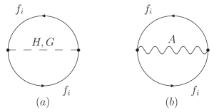
Figure 4: The two loop fermionic contribution to the effective potential. Due to the HLET, differentiation with respect to the Higges VEV $v$ provides the one-, two-, three- and four-Higgs Green functions (at zero momentum).

Due to the HLET, from the diagrams contributing to the effective potential we can extract information about the Higgs tadpole, mass, tri- and quadri-linear couplings, by simply differentiating with respect to $v$. Moreover, since we are interested only in the contributions which depend on the Yukawa couplings, we only need to consider the two-loop fermionic effective potential contributions, shown in Fig. 4. Introducing the integrals

$$K_{ijk} = \mu^{2\epsilon}\int\!\frac{d^{d}k}{(2\pi)^{d}}\int\!\frac{d^{d}\ell}{(2\pi)^{d}}\frac{1}{(k^{2}-m^{2}_{i})(\ell^{2}-m^{2}_{j})[(k+\ell)^{2}-m^{2}_{k}]}$$

$$= -\frac{1}{(4\pi)^{4}}\sum_{n=i,j,k}m^{2}_{n}\left[\frac{2}{\epsilon^{2}}-\frac{2}{\epsilon}\left(\ln\frac{m^{2}_{n}}{\bar{\mu}^{2}}-\frac{3}{2}\right)\right]+\dots,$$

$$L_{ij} = \mu^{2\epsilon}\int\!\frac{d^{d}k}{(2\pi)^{d}}\int\!\frac{d^{d}\ell}{(2\pi)^{d}}\frac{1}{(k^{2}-m^{2}_{i})(\ell^{2}-m^{2}_{j})}$$ (85)

$$= -\frac{1}{(4\pi)^{4}}m_{i}^{2}m_{j}^{2}\left[\frac{4}{\epsilon^{2}}+\frac{2}{\epsilon}\left(2-\ln\frac{m^{2}_{i}}{\bar{\mu}^{2}}-\ln\frac{m^{2}_{j}}{\bar{\mu}^{2}}\right)\right]+\dots,$$

where $\ln\bar{\mu}^{2}=\ln(4\pi\mu^{2})-\gamma_{E}$, and the dots stand for finite parts, one finds

$$(a)|_{H} = -\frac{i}{2}h_{i}^{2}d\Bigg{[}L_{Hf_{i}}-\frac{1}{2}L_{f_{i}f_{i}}+\Bigg{(}2m^{2}_{i}-\frac{1}{2}m^{2}_{H}\Bigg{)}K_{Hf_{i}f_{i}}\Bigg{]},$$

$$(a)|_{G} = -\frac{i}{2}h_{i}^{2}d\Bigg{[}L_{Gf_{i}}-\frac{1}{2}L_{f_{i}f_{i}}-\frac{1}{2}m^{2}_{G}K_{Gf_{i}f_{i}}\Bigg{]},$$

$$(b) = -i\frac{g^{2}}{4}d(d-2)\Bigg{[}L_{Af_{i}}-\frac{1}{2}L_{f_{i}f_{i}}+\Bigg{(}m^{2}_{i}-\frac{1}{2}m^{2}_{A}\Bigg{)}K_{Af_{i}f_{i}}\Bigg{]}$$ (86)

$$+\frac{i}{4}h_{i}^{2}d\left[m^{2}_{A}K_{af_{i}f_{i}}-m^{2}_{c}K_{cf_{i}f_{i}}\right].$$

The contributions to $\overline{\Gamma^{(2)}_{H^{4}}}$ which depend on the Yukawa couplings are simply obtained by differentiating the above expressions four times with respect to $v$. As far as the term $\overline{D^{(1)}\Gamma^{(1)}_{H^{4}}}$ is concerned, one can use the results of Appendix A for the one-loop effective potential and renormalization constants (notice that in this case, one cannot limit one’s attention to the fermionic contributions only, due to the dependence on the Yukawa couplings of the renormalization constants).

The combination of these two terms leads to a massive cancellation, yielding finally

$$\frac{\partial}{\partial\xi}Z^{(2)}_{H,h_{i}}=-\frac{2g^{2}}{(4\pi)^{4}\epsilon}\sum_{i}h^{2}_{i},$$ (87)

thus establishing the GFP-dependence of $Z^{(2)}_{H,h_{i}}$ in the $\overline{R_{\xi}}$ gauges.

As a check for the consistency of the procedure, we can evaluate the full two-loop Higgs wave-function renormalization constant $Z^{(2)}_{H}$ of our model, through the direct calculation of the relevant Feynman diagrams of the Higgs-boson self-energy, shown in Fig. 5. As mentioned earlier, we will calculate in the symmetric phase, $v=0$, keeping only contributions proportional to the Yukawa couplings $h_{i}$

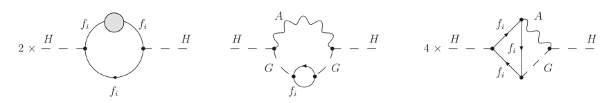
Figure 5: Fermion diagrams contributing $g^{2}\sum_{i}h_{i}^{2}$ terms to the two-loop Higgs wave-function renormalization constant $Z^{(2)}_{H}$ in the symmetric phase.

We will use directly the $D$-formalism to explicitly check that all overlapping divergences cancel, and to get the fermionic contributions to $Z^{(2)}_{H}$ through the formula

$$Z^{(2)}_{H}=\frac{i}{2}\frac{\partial}{\partial p^{2}}\left.\left\{\overline{D^{(1)}\Gamma^{(1)}_{H^{2}}(x_{\rm R};\mu,\epsilon)}+\overline{\Gamma^{(2)}_{H^{2}}(x_{\rm R};\mu,\epsilon)}\right\}\right|_{\sigma_{\rm R}=1,\,p^{2}=0}.$$ (88)

Once again one should keep in mind that $\Gamma^{(1)}_{H^{2}}$ must be calculated at a general value of $\sigma$ (which means that the ($\sigma-1$) part of the $A_{\mu}GH$ vertex will also contribute). The final result is given by

$$\mu^{\epsilon}Z^{(2)}_{H,h_{i}}=\frac{-2g^{2}(\xi+4)\sum_{i}h_{i}^{2}+8\sum_{i}h_{i}^{4}}{(4\pi)^{4}\epsilon}-\frac{8\sum_{i}h_{i}^{4}}{(4\pi)^{4}\epsilon^{2}}\ ,$$ (89)

which coincides with (87) after differentiating with respect to $\xi$. From this expression one can determine the two-loop anomalous dimension of the Higgs field, which is given by Machacek:1983tz

$$\gamma^{(2)}_{H} = -\frac{1}{2}\sum_{n}\rho_{n}x_{n}\frac{\partial}{\partial x_{n}}C_{H}^{1},$$ (90)

where $x_{n}$ denotes collectively the free parameters of the theory, $\rho_{n}\epsilon$ their mass-dimension, and $C^{1}_{H}$ the coefficient of the simple pole of the Higgs 1PI self-energy. Therefore

$$\gamma^{(2)}_{H,h_{i}} = -\frac{1}{2}\left(\lambda\frac{\partial}{\partial\lambda}+\frac{1}{2}g\frac{\partial}{\partial g}+\frac{1}{2}\sum_{i}h_{i}\frac{\partial}{\partial h_{i}}\right)C^{1}_{H,h_{i}}$$ (91)

$$= \frac{2g^{2}(\xi+4)\sum_{i}h_{i}^{2}-8\sum_{i}h_{i}^{4}}{(4\pi)^{4}}\ .$$

Evidently, despite the fact that $\Delta v=0$ exactly, the two-loop running of $\tan\beta$ turns out to be GFP-dependent.

VII Conclusions

We have developed a new formalism for determining the renormalization and the GFP-dependence of Green functions to all orders in perturbation theory. The formalism makes use of the fact that the renormalized Green functions are obtained by displacing both the unrenormalized fields and fundamental parameters of the theory with respect to the renormalized ones. Due to this property, we have called it the displacement operator formalism or, in short, the $D$-formalism. With the help of this formalism the CTs necessary for the renormalization of any Green function can be unambiguously determined, to any given order of perturbation theory. In particular, if one applies the $D$-operator before integrating over the loop momenta, one can systematically generate all the CTs that would have been obtained in the conventional diagrammatic framework. We explicitly demonstrate the full potential of the $D$-formalism by considering several known examples of renormalization of theories up to 2-loops, such as a $\phi^{4}$-theory, QED, and QCD in the BFM $R_{\xi}$ gauge.

One of the great advantages of the $D$-formalism is that it can be used to calculate the precise form of deformation of symmetries, which are modified in the process of renormalization, such as the NI. Hence, the dependence of the renormalized Green functions on the renormalized GFPs can be computed exactly, thereby offering a new method for evaluating the GFP-dependence within a given scheme of renormalization, e.g., the $\overline{\rm MS}$ scheme, the OS scheme, etc. Given that a concrete, closed formula describing the deformation of the NI to all orders exists now, one should be able to conclusively settle various formal issues related to gauge-invariance. Most notably, it would be interesting to revisit the important question of the all-order gauge-invariance of the pole of the unstable particles, together with other topics related to the gauge-invariant formulation of resonant transition amplitudes Papavassiliou:1995fq .

In theories with SSB, in addition to the Slavnov–Taylor identities and the NI, the HLET plays an important role as well. The ordinary $R_{\xi}$ gauge violates the HLET for off-shell 1PI correlation functions. In order to explore the constraints imposed by the HLET we have resorted to a toy field theory with SSB, the Abelian Higgs model, which was quantized using a HLET-preserving gauge. An important consequence of these gauges is that the VEV $v$ of a Higgs field renormalizes multiplicatively by the Higgs wavefunction, so there is no additional UV infinite shift to $v$, i.e. $\Delta v_{\rm div}=0$. Employing the $D$-formalism in the context of a HLET-preserving gauge, we have shown that the fundamental quantity $\tan\beta$, defined in the two-Higgs models, is GFP-dependent at two loops, exactly as happens for the usual $R_{\xi}$ gauge, in which there exist additional UV infinite shifts to the Higgs VEVs. The analysis presented here strongly suggests that the $\tan\beta$ cannot be made gauge-independent within the framework of conventional Green functions, even if the gauge-fixing employed respects all relevant symmetries and constraints, such as the HLET. These results motivate one to explore the possibility of defining $\tan\beta$ at higher orders through the GFP-independent effective Green functions constructed by means of the pinch technique Cornwall:1981zr . In particular, it would be interesting to extend the concept and construction of the Higgs-boson effective charge Papavassiliou:1997fn to the case of multi-Higgs models, and more specifically to supersymmetric theories. We hope to be able to report progress on this subjects in the near future.

The formulation developed in this article presents novel perspectives for the study of several other known topics. Specifically, the $D$-formalism may be used to systematically investigate the renormalization-scheme dependence of 1PI correlation functions. It may also be employed to algebraically determine the restoring terms of a “bad” UV regularizing scheme, i.e., a scheme that does not preserve the Slavnov–Taylor identities. Since it provides all-order information on the renormalization of Green functions under study, it might be useful in controlling the calculation of non-perturbative effects, such as those related to the dynamics of renormalons Lautrup:1977hs .

The $D$-formalism can be straightforwardly extended to systematize the procedure of renormalizing non-renormalizable field theories. In particular, it may be used to organize the infinite series of CTs needed to renormalize such theories. But even in the case of renormalizable perturbative field theories the $D$-formalism can be automated, for example with the aid of a computational package, to reliably compute all the CTs required for the renormalization of 1PI correlation functions at high orders. It would therefore be interesting to explore these new horizons opening up, embarking into a study of the onset of non-perturbative dynamics at very high orders of perturbation theory LeGuillou:1990nq .

Appendix A Feynman rules and renormalization of the Abelian Higgs model

The Feynman rules derived from the Lagrangian density given in (V) are listed in Fig. 6.

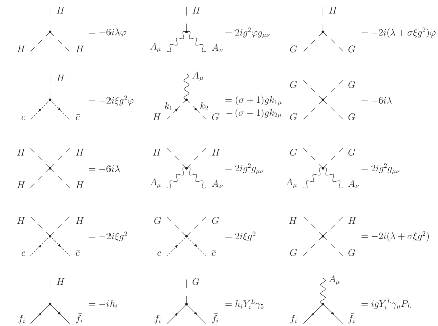
Figure 6: The Feynman rules for the Abelian Higgs model in the HLET type of gauge.

The model can be renormalized with the renormalization condition $\sigma_{\mathrm{R}}=1$, by introducing the following renormalization constants

$$H=Z_{H}^{\frac{1}{2}}H_{\mathrm{R}},\qquad G=Z_{G}^{\frac{1}{2}}G_{\mathrm{R}},\qquad A^{\mu}=Z_{A}^{\frac{1}{2}}A^{\mu}_{\mathrm{R}},\qquad\bar{c}c=Z_{c}\bar{c}_{\mathrm{R}}c_{\mathrm{R}},\qquad v=Z_{H}^{\frac{1}{2}}v_{\mathrm{R}},$$

$$m^{2}=Z_{m^{2}}m^{2}_{\mathrm{R}},\qquad\lambda=Z_{\lambda}\lambda_{\mathrm{R}},\qquad\quad g=Z_{g}g_{\mathrm{R}},\qquad\quad\xi=Z_{\xi}\xi_{\mathrm{R}},\qquad\quad\sigma=Z_{\sigma}\sigma_{\mathrm{R}},$$

$$f^{L}_{i}=(Z_{i}^{L})^{\frac{1}{2}}f^{L}_{i{\rm R}},\qquad f^{R}_{i}=(Z_{i}^{R})^{\frac{1}{2}}f^{R}_{i{\rm R}}\qquad h_{i}=Z_{h_{i}}h^{\mathrm{R}}_{i}\;.$$ (92)

Notice that left and right fermions get renormalized with different renormalization constants.

The determination of the renormalization constant above, is simplified, due to the HLET: for example, the knowledge of the fermion self-energy will automatically imply the knowledge of the Higgs-fermion-fermion vertex through the differentiation of the former with respect to the Higgs vev $v$ (notice that, in this particular case, we would find immediately that this vertex is one-loop finite within the HLET gauges).

In table 1, we report all the divergent parts for the one-loop Green functions of the model.

$\overline{\Gamma}$	$\frac{i}{(4\pi)^{2}\epsilon}\frac{1}{2}\left\{\left(10\lambda^{2}+2\xi g^{2}\lambda+3g^{4}-4\sum_{i}h_{i}^{4}\right)v^{4}+\left(8\lambda+2\xi g^{2}\right)m^{2}v^{2}+2m^{4}\right\}$
$\overline{\Gamma_{H}}$	$\frac{2i}{(4\pi)^{2}\epsilon}\left\{\left(10\lambda^{2}+2\xi g^{2}\lambda+3g^{4}-4\sum_{i}h_{i}^{4}\right)v^{3}+\left(4\lambda+\xi g^{2}\right)m^{2}v\right\}$
$\overline{\Gamma_{H^{2}}}$	$\frac{-i}{(4\pi)^{2}\epsilon}\left\{\left[(6+2\xi)g^{2}-4\sum_{i}h_{i}^{2}\right]q^{2}\right.$
	$\left.-(8\lambda+2\xi g^{2})m^{2}-\left(60\lambda^{2}+12\lambda\xi g^{2}+18g^{4}-24\sum_{i}h_{i}^{4}\right)v^{2}\right\}$
$\overline{\Gamma_{G^{2}}}$	$\frac{i}{(4\pi)^{2}\epsilon}\left\{\left[6(\xi-1)g^{2}+4\sum_{i}h_{i}^{2}\right]q^{2}\right.$
	$+\left.(8\lambda-6\xi g^{2})m^{2}+\left(20\lambda^{2}+4\lambda\xi g^{2}+6g^{4}+6\xi^{2}g^{4}-8\sum_{i}h_{i}^{4}\right)v^{2}\right\}$
$\overline{\Gamma_{A_{\mu}A_{\nu}}}$	$\frac{i}{(4\pi)^{2}\epsilon}\left\{\left[-\frac{10}{3}g^{2}q^{2}-2\left(3g^{2}+\xi g^{2}-2\sum_{i}h_{i}^{2}\right)g^{2}v^{2}\right]g_{\mu\nu}+\frac{16}{3}g^{2}q_{\mu}q_{\nu}\right\}$
$\overline{\Gamma_{A_{\mu}G}}$	$\frac{2}{(4\pi)^{2}\epsilon}\left\{2\lambda+3\xi g^{2}-3g^{2}+2\sum_{i}h_{i}^{2}\right\}gvq_{\mu}$
$\overline{\Gamma_{c\bar{c}}}$	$\frac{i}{(4\pi)^{2}\epsilon}\left\{4\lambda\xi g^{2}+6\xi^{2}g^{4}\right\}v^{2}$
$\overline{\Gamma_{f_{i}\bar{f}_{i}}}$	$\frac{i}{(4\pi)^{2}\epsilon}\left\{q/P_{L}(2g^{2}\xi+2h_{i}^{2})+q/P_{R}(2h_{i}^{2})\right\}$
$\overline{\Gamma_{H^{3}}}$	$\frac{12i}{(4\pi)^{2}\epsilon}\left\{10\lambda^{2}+2\lambda\xi g^{2}+3g^{4}-4\sum_{i}h_{i}^{4}\right\}v$	$\overline{\Gamma_{HA_{\mu}A_{\nu}}}$	$\frac{-4i}{(4\pi)^{2}\epsilon}\left\{3g^{2}+\xi g^{2}-2\sum_{i}h_{i}^{2}\right\}g^{2}vg_{\mu\nu}$
$\overline{\Gamma_{H^{4}}}$	$\frac{12i}{(4\pi)^{2}\epsilon}\left\{10\lambda^{2}+2\lambda\xi g^{2}+3g^{4}-4\sum_{i}h_{i}^{4}\right\}$	$\overline{\Gamma_{H^{2}A_{\mu}A_{\nu}}}$	$\frac{-4i}{(4\pi)^{2}\epsilon}\left\{3g^{2}+\xi g^{2}-2\sum_{i}h_{i}^{2}\right\}g^{2}g_{\mu\nu}$
$\overline{\Gamma_{G^{4}}}$	$\frac{12i}{(4\pi)^{2}\epsilon}\left\{10\lambda^{2}-6\lambda\xi g^{2}+3g^{4}-4\sum_{i}h_{i}^{4}\right\}$	$\overline{\Gamma_{G^{2}A_{\mu}A_{\nu}}}$	$\frac{-4i}{(4\pi)^{2}\epsilon}\left\{3\left(1-\xi\right)g^{2}-2\sum_{i}h_{i}^{2}\right\}g^{2}g_{\mu\nu}$
$\overline{\Gamma_{HG^{2}}}$	$\frac{4i}{(4\pi)^{2}\epsilon}\left\{10\lambda^{2}+2\lambda\xi g^{2}+3g^{4}\right.$	$\overline{\Gamma_{Hc\bar{c}}}$	$\frac{4i}{(4\pi)^{2}\epsilon}\left\{2\lambda\xi g^{2}+3\xi^{2}g^{4}\right\}v$
	$\left.+3\xi^{2}g^{4}-4\sum_{i}h_{i}^{4}\right\}v$
$\overline{\Gamma_{H^{2}G^{2}}}$	$\frac{4i}{(4\pi)^{2}\epsilon}\left\{10\lambda^{2}+2\lambda\xi g^{2}+3g^{4}+3\xi^{2}g^{4}-4\sum_{i}h_{i}^{4}\right\}$	$\overline{\Gamma_{H^{2}c\bar{c}}}$	$\frac{4i}{(4\pi)^{2}\epsilon}\left\{2\lambda\xi g^{2}+3\xi^{2}g^{4}\right\}$
$\overline{\Gamma_{A_{\mu}HG}}$	$\frac{-2g}{(4\pi)^{2}\epsilon}\left\{\left(2\lambda+\xi g^{2}+3g^{2}-2\sum_{i}h_{i}^{2}\right)k_{1\mu}\right.$	$\overline{\Gamma_{G^{2}c\bar{c}}}$	$\frac{-4i}{(4\pi)^{2}\epsilon}\left\{2\lambda\xi g^{2}-\xi^{2}g^{4}\right\}$
	$\left.-\left(2\lambda+3\xi g^{2}-3g^{2}+2\sum_{i}h_{i}^{2}\right)k_{2\mu}\right\}$

Table 1: The one-loop divergent parts of the Green functions of the Abelian Higgs model in the HLET preserving gauge (with $\sigma=1$).

Using these results, one finds

$$\mu^{\epsilon}Z_{H} = 1+\frac{(6+2\xi)g^{2}-4\sum_{i}h_{i}^{2}}{(4\pi)^{2}\epsilon}\ ,$$

$$\mu^{\epsilon}Z_{G} = 1+\frac{(6-6\xi)g^{2}-4\sum_{i}h_{i}^{2}}{(4\pi)^{2}\epsilon}\ ,$$

$$\mu^{\epsilon}Z_{A} = 1+\frac{-\frac{10}{3}g^{2}}{(4\pi)^{2}\epsilon}\ ,$$

$$\mu^{\epsilon}Z_{c} = 1\;,$$

$$\mu^{\epsilon}Z_{i}^{L} = 1+\frac{-2g^{2}\xi-2h_{i}^{2}}{(4\pi)^{2}\epsilon}\ ,$$

$$\mu^{\epsilon}Z_{i}^{R} = 1+\frac{-2h_{i}^{2}}{(4\pi)^{2}\epsilon}\ ,$$

$$Z_{m^{2}} = 1+\frac{(8\lambda-6g^{2}+4\sum_{i}h_{i}^{2})}{(4\pi)^{2}\epsilon}\ ,$$

$$\mu^{-\epsilon}Z_{\lambda} = 1+\frac{20\lambda-12g^{2}+8\sum_{i}h_{i}^{2}+\frac{6}{\lambda}g^{4}-\frac{8}{\lambda}\sum_{i}h_{i}^{4}}{(4\pi)^{2}\epsilon}\ ,$$

$$\mu^{-\frac{\epsilon}{2}}Z_{g} = 1+\frac{\frac{5}{3}g^{2}}{(4\pi)^{2}\epsilon}\ ,$$

$$\mu^{-\frac{\epsilon}{2}}Z_{h_{i}} = 1+\frac{-3g^{2}+2h_{i}^{2}+2\sum_{j=1}^{2}h_{j}^{2}}{(4\pi)^{2}\epsilon}\ ,$$

$$Z_{\xi} = 1+\frac{4\lambda+4\xi g^{2}-\frac{28}{3}g^{2}+4\sum_{i}h_{i}^{2}}{(4\pi)^{2}\epsilon}\ ,$$

$$Z_{\sigma} = 1+\frac{4\lambda+(-6+6\xi)g^{2}+4\sum_{i}h_{i}^{2}}{(4\pi)^{2}\epsilon}\ .$$ (93)

Notice that $Z_{A}^{\frac{1}{2}}Z_{g}=1$ as it should due to the Ward identities of the theory. Combining the divergent parts of the Green functions given in table 1, together with the above renormalization constants, one can explicitly check the validity of the renormalized NI of Eq.(62) at one loop.

The effective potential is particularly useful in the context of the HLET-preserving gauges, furnishing a substantial amount of information with relatively moderate effort Kastening:1993zn . In dimensional regularization, the one-loop effective potential reads

$$V^{(1)} = \frac{i}{4(4\pi^{2})}\Bigg{[}{m^{4}_{H}}\left(\frac{3}{2}-\ln\frac{m^{2}_{H}}{\bar{\mu}^{2}}\right)+{m^{4}_{G}}\left(\frac{3}{2}-\ln\frac{m^{2}_{G}}{\bar{\mu}^{2}}\right)+{m^{4}_{A}}\left(\frac{5}{2}-3\ln\frac{m^{2}_{A}}{\bar{\mu}^{2}}\right)$$ (94)

$$+\,\frac{m^{4}_{c}}{\sigma^{2}}\left(\frac{3}{2}-\ln\frac{m^{2}_{c}}{\sigma^{2}\bar{\mu}^{2}}\right)-2m^{2}_{c}\left(\frac{3}{2}-\ln\frac{m^{2}_{c}}{\bar{\mu}^{2}}\right)-4\sum_{i}m^{4}_{i}\left(1-\ln\frac{m^{2}_{i}}{\bar{\mu}^{2}}\right)\Bigg{]}$$

$$+\>\frac{i}{2(4\pi)^{2}\epsilon}\Bigg{(}m^{4}_{H}+m^{4}_{G}+3m^{4}_{A}+\frac{m_{c}^{4}}{\sigma^{2}}-2m_{c}^{4}-\sum_{i}m^{4}_{i}\Bigg{)}\;,$$

where $\ln\bar{\mu}^{2}=\ln(4\pi\mu^{2})-\gamma_{E}$. As stated earlier it is important to keep explicitly the dependence on $\sigma$, since this will play a crucial role in cancelling the overlapping divergences in our two-loop expressions, when the $D$-formalism is applied after integration.

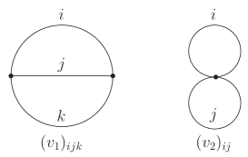
Figure 7: Topologies contributing to the two loop effective potential. $i$, $j$, and $k$ labels all the possible field combinations allowed by the Feynman rules.

At two loops, there are two basic topologies contributing to the effective potential, shown in Fig. 7. It turns out that all these two loop diagrams can be expressed in terms of the integrals $L_{ij}$ and $K_{ijk}$ introduced in Eq.(85). In table 2 we report the results of the (scalar and vector) diagrams.

$(v_{1})_{H^{3}}$	$3iv^{2}\lambda^{2}K_{HHH}$
$(v_{1})_{HG^{2}}$	$iv^{2}(\lambda+\xi g^{2})^{2}K_{HGG}$
$(v_{1})_{Hc\bar{c}}$	$-2iv^{2}\xi^{2}g^{4}K_{Hc\bar{c}}$
$(v_{1})_{HAG}$	$2ig^{2}\left\{m^{2}_{H}K_{HAG}+L_{AG}+\frac{1}{2}\xi L_{Gc}-\frac{1}{2}L_{GA}-\frac{1}{4}(1-\xi)\left[L_{cG}+L_{HG}-L_{cH}\right.\right.$
	$\left.(2m^{2}_{G}-2m^{2}_{H}-m^{2}_{c}-m^{2}_{A})K_{HGc}\right]+\frac{m^{2}_{G}-m^{2}_{H}-m^{2}_{A}}{4m^{2}_{A}}\left[L_{GA}+L_{Hc}-L_{HA}-L_{Gc}\right]$
	$-\frac{(m^{2}_{G}-m^{2}_{H}-m^{2}_{A})^{2}}{4m^{2}_{A}}\left[K_{HGA}-K_{HGc}\right]\big{\}}$
$(v_{1})_{HA^{2}}$	$iv^{2}g^{4}\big{\{}(d-2)K_{HAA}+2\xi K_{HAc}-\frac{1}{2m^{2}_{A}}(1-\xi)[L_{cA}+L_{Hc}-L_{cc}-L_{HA}]+\frac{1}{2}(1-\xi)^{2}K_{Hcc}$
	$+\frac{m^{2}_{H}-2m^{2}_{A}}{4m^{4}_{A}}[L_{AA}+L_{cc}-2L_{Ac}]+\frac{1}{2m^{2}_{A}}(1-\xi)(3m^{2}_{A}-2m^{2}_{H}+m^{2}_{c})\left[K_{HAc}-K_{Hcc}\right]$
	$+\frac{(m^{2}_{H}-2m^{2}_{A})^{2}}{4m^{4}_{A}}\left[K_{HAA}+K_{Hcc}-2K_{HAc}\right]\big{\}}$
$(v_{2})_{H^{2}}$	$i\frac{3\lambda}{4}L_{HH}$	$(v_{2})_{G^{2}}$	$i\frac{3\lambda}{4}L_{GG}$
$(v_{2})_{HG}$	$i\frac{\lambda+\xi g^{2}}{2}L_{HG}$	$(v_{2})_{GA}$	$i\frac{g^{2}}{2}\big{\{}(d-1)L_{GA}+\xi L_{Gc}\big{\}}$
$(v_{2})_{Hc}$	$-i\xi g^{2}L_{Hc}$	$(v_{2})_{Gc}$	$i\xi g^{2}L_{Gc}$

Table 2: Scalar and vector two loop contributions to the effective potential (with $\sigma=1$). The fermionic contributions are given in Eq.(86) of the text.

Using these results in conjunction with Eq.(84), one can obtain the full gauge-dependence of the two-loop Higgs wave-function renormalization and anomalous dimension. Specifically,

$$\frac{\partial}{\partial\xi}Z^{(2)}_{H} = \frac{-2g^{2}\sum_{i}h^{2}_{i}-4\lambda g^{2}-6\xi g^{4}+2g^{4}}{(4\pi)^{4}\epsilon}+\frac{8\lambda g^{2}+24\xi g^{4}}{(4\pi)^{4}\epsilon^{2}},$$

$$\frac{\partial}{\partial\xi}\gamma^{(2)}_{H} = \frac{2g^{2}\sum_{i}h^{2}_{i}+4\lambda g^{2}+6\xi g^{4}-2g^{4}}{(4\pi)^{4}\epsilon}\;.$$ (95)

We end by reporting for completeness the full two-loop Higgs wave function renormalization and anomalous dimension:

$$\mu^{\epsilon}Z^{(2)}_{H} = \frac{-4\lambda-4\lambda\xi g^{2}+(-2+2\xi-3\xi^{2})g^{4}-2\xi g^{2}\sum_{i}h_{i}^{2}-8g^{2}\sum_{i}h_{i}^{2}+8\sum_{i}h_{i}^{4}}{(4\pi)^{4}\epsilon}$$

$$+ \frac{8\lambda\xi g^{2}+(12+12\xi^{2})g^{4}-12g^{2}\sum_{i}h_{i}^{2}-8\sum_{i}h_{i}^{4}}{(4\pi)^{4}\epsilon^{2}},$$

$$\gamma^{(2)}_{H} = \frac{2\lambda+(3\xi^{2}-2\xi+2)g^{4}+4\lambda\xi g^{2}+2g^{2}(\xi+4)\sum_{i}h_{i}^{2}-8\sum_{i}h_{i}^{4}}{(4\pi)^{4}}\;.$$ (96)

References

- (1) J. S. Schwinger, Phys. Rev. 73 (1948) 416; Phys. Rev. 74 (1948) 1439.
- (2) R. P. Feynman, Phys. Rev. 74 (1948) 1430; Rev. Mod. Phys. 20, 367 (1948).
- (3) F. J. Dyson, Phys. Rev. 75 (1949) 486.
- (4) N. N. Bogoliubov and O. S. Parasiuk, Acta Math. 97 (1957) 227.
- (5) K. Hepp, Commun. Math. Phys. 2 (1966) 301.
- (6) W. Zimmermann, Commun. Math. Phys. 15 (1969) 208 [Lect. Notes Phys. 558 (2000) 217]; Annals Phys. 77 (1973) 536 [Lect. Notes Phys. 558 (2000) 244].
- (7) K. Symanzik, Commun. Math. Phys. 18 (1970) 227.
- (8) H. Epstein and V. Glaser, Annales Poincare Phys. Theor. A 19 (1973) 211.
- (9) G. ’t Hooft and M. J. G. Veltman, Nucl. Phys. B 44, 189 (1972).
- (10) G. ’t Hooft, Nucl. Phys. B 33 (1971) 173; Nucl. Phys. B 35, 167 (1971); Nucl. Phys. B 61 (1973) 455.
- (11) B. W. Lee and J. Zinn-Justin, Phys. Rev. D 5 (1972) 3137.
- (12) C. Becchi, A. Rouet and R. Stora, Commun. Math. Phys. 42, 127 (1975).
- (13) O. Piguet and S. P. Sorella, Lect. Notes Phys. M28, 1 (1995).
- (14) E. Kraus, Annals Phys. 262, 155 (1998) [arXiv:hep-th/9709154].
- (15) P. A. Grassi, T. Hurth and M. Steinhauser, Annals Phys. 288, 197 (2001) [arXiv:hep-ph/9907426].
- (16) B. S. Dewitt, Phys. Rev. 162, 1195 (1967).
- (17) G. ’t Hooft, In *Karpacz 1975, Proceedings, Acta Universitatis Wratislaviensis No.368, Vol.1*, Wroclaw 1976, 345-369.
- (18) L. F. Abbott, Nucl. Phys. B 185, 189 (1981).
- (19) D. M. Capper and A. MacLean, Nucl. Phys. B 203, 413 (1982).
- (20) L. F. Abbott, M. T. Grisaru and R. K. Schaefer, Nucl. Phys. B 229, 372 (1983).
- (21) N. K. Nielsen, Nucl. Phys. B 97, 527 (1975).
- (22) H. Kluberg-Stern and J. B. Zuber, Phys. Rev. D 12, 467 (1975); Phys. Rev. D 12, 482 (1975).
- (23) O. Piguet and K. Sibold, Nucl. Phys. B 253, 517 (1985).
- (24) I. J. R. Aitchison and C. M. Fraser, Annals Phys. 156, 1 (1984); D. Johnston, Nucl. Phys. B 253, 687 (1985); Nucl. Phys. B 283, 317 (1987); O. M. Del Cima, D. H. T. Franco and O. Piguet, Nucl. Phys. B 551, 813 (1999); O. M. Del Cima, Phys. Lett. B 457, 307 (1999); J. Bernabeu, J. Papavassiliou and D. Binosi, arXiv:hep-ph/0405288.
- (25) C. Becchi, A. Rouet and R. Stora, Annals Phys. 98, 287 (1976); I. V. Tyutin, LEBEDEV-75-39.
- (26) P. Gambino and P. A. Grassi, Phys. Rev. D 62, 076002 (2000) [arXiv:hep-ph/9907254].
- (27) B. M. Kastening, Phys. Rev. D 51, 265 (1995) [arXiv:hep-ph/9307220].
- (28) J. R. Ellis, M. K. Gaillard and D. V. Nanopoulos, Nucl. Phys. B 106, 292 (1976).
- (29) M. A. Shifman, A. I. Vainshtein and V. I. Zakharov, Phys. Lett. B 78, 443 (1978).
- (30) M. A. Shifman, A. I. Vainshtein, M. B. Voloshin and V. I. Zakharov, Sov. J. Nucl. Phys. 30, 711 (1979) [Yad. Fiz. 30, 1368 (1979)].
- (31) A. I. Vainshtein, V. I. Zakharov and M. A. Shifman, Sov. Phys. Usp. 23 (1980) 429 [Usp. Fiz. Nauk 131 (1980) 537]; M. B. Voloshin, Sov. J. Nucl. Phys. 44, 478 (1986) [Yad. Fiz. 44, 738 (1986)]; M. A. Shifman, Phys. Rept. 209, 341 (1991) [Sov. Phys. Usp. 32, 289 (1989 UFNAA,157,561-598.1989)].
- (32) S. Dawson and H. E. Haber, Int. J. Mod. Phys. A 7, 107 (1992).
- (33) A. A. Slavnov, Theor. Math. Phys. 10, 99 (1972) [Teor. Mat. Fiz. 10, 153 (1972)]; J. C. Taylor, Nucl. Phys. B 33, 436 (1971).
- (34) A. Pilaftsis, Phys. Lett. B 422, 201 (1998) [arXiv:hep-ph/9711420].
- (35) K. Fujikawa, B. W. Lee and A. I. Sanda, Phys. Rev. D 6, 2923 (1972).
- (36) M. Bohm, H. Spiesberger and W. Hollik, Fortsch. Phys. 34 (1986) 687.
- (37) P. H. Chankowski, S. Pokorski and J. Rosiek, Phys. Lett. B 274, 191 (1992); Phys. Lett. B 286, 307 (1992); Nucl. Phys. B 423, 437 (1994) [arXiv:hep-ph/9303309].
- (38) W. Marciano and A. Sirlin, Nucl. Phys. B 88, 86 (1975); W. Bardeen, A.J. Buras, D.W. Duke and T. Muta, Phys. Rev. D 18, 3998 (1978).
- (39) J. Papavassiliou and A. Pilaftsis, Phys. Rev. Lett. 80, 2785 (1998) [arXiv:hep-ph/9710380]; Phys. Rev. D 58, 053002 (1998) [arXiv:hep-ph/9710426].
- (40) J. F. Gunion, H. E. Haber, G. L. Kane and S. Dawson, “The Higgs Hunter’s Guide,” SCIPP-89/13
- (41) H. E. Haber, G. L. Kane and T. Sterling, Nucl. Phys. B 161, 493 (1979); N. G. Deshpande and E. Ma, Phys. Rev. D 18, 2574 (1978); J. F. Donoghue and L. F. Li, Phys. Rev. D 19, 945 (1979); L. F. Abbott, P. Sikivie and M. B. Wise, Phys. Rev. D 21, 1393 (1980); B. McWilliams and L. F. Li, Nucl. Phys. B 179, 62 (1981); J. F. Gunion and H. E. Haber, Nucl. Phys. B 272, 1 (1986) [Erratum-ibid. B 402, 567 (1993)].
- (42) Y. Yamada, Phys. Lett. B 530, 174 (2002) [arXiv:hep-ph/0112251]; arXiv:hep-ph/0210324.
- (43) A. Freitas and D. Stockinger, Phys. Rev. D 66, 095014 (2002) [arXiv:hep-ph/0205281].
- (44) Although it is easy to incorporate in our formalism, we will not consider for simplicity the cosmological constant, which only becomes relevant to the renormalization of vacuum energy graphs.
- (45) If there is mixing between different types of fields , the first term should be replaced by , with .
- (46) Up to two loops, this is not such a serious complication, since one needs the explicit dependence of one-loop diagrams only.
- (47) C. Itzykson and J. B. Zuber, Quantum Field Theory.
- (48) S. Weinberg, The Quantum Theory of Fields (Cambridge University Press, New York, 1996), Vol. II.
- (49) J. Papavassiliou, Phys. Rev. D 51, 856 (1995) [arXiv:hep-ph/9410385].
- (50) In general, there could be more than one GFPs, and correspondingly more than one associate BRS sources need be included to study the dependence of the Green functions on the additional GFPs, see R. Häußling and E. Kraus, Z. Phys. C 75, 739 (1997) [arhiv:hep-th/9608160].
- (51) R. G. Stuart, Phys. Lett. B 262, 113 (1991).
- (52) A. Sirlin, Phys. Rev. Lett. 67, 2127 (1991).
- (53) In the presence of mixing of different fields, the wavefunction renormalizations are to be replaced by matrices of the form .
- (54) M. E. Machacek and M. T. Vaughn, Nucl. Phys. B 222, 83 (1983); Nucl. Phys. B 236, 221 (1984); Nucl. Phys. B 249, 70 (1985).
- (55) J. Papavassiliou and A. Pilaftsis, Phys. Rev. Lett. 75, 3060 (1995) [arXiv:hep-ph/9506417]; Phys. Rev. D 53, 2128 (1996) [arXiv:hep-ph/9507246]; Phys. Rev. D 54, 5315 (1996) [arXiv:hep-ph/9605385].
- (56) J. M. Cornwall, Phys. Rev. D 26, 1453 (1982); J. M. Cornwall and J. Papavassiliou, Phys. Rev. D 40, 3474 (1989); D. Binosi and J. Papavassiliou, Phys. Rev. D 66, 111901 (2002) [arXiv:hep-ph/0208189]; J. Phys. G 30, 203 (2004) [arXiv:hep-ph/0301096]; D. Binosi, J. Phys. G 30, 1021 (2004) [arXiv:hep-ph/0401182].
- (57) B. Lautrup, Phys. Lett. B 69, 109 (1977); G. Parisi, Phys. Lett. B 76, 65 (1978); Nucl. Phys. B 150, 163 (1979); F. David, Nucl. Phys. B 234, 237 (1984); A. H. Mueller, Nucl. Phys. B 250, 327 (1985); V. I. Zakharov, Nucl. Phys. B 385, 452 (1992); D. J. Broadhurst, Z. Phys. C 58, 339 (1993); M. Neubert and C. T. Sachrajda, Nucl. Phys. B 438, 235 (1995) [arXiv:hep-ph/9407394]; M. Dasgupta and B. R. Webber, Phys. Lett. B 382, 273 (1996) [arXiv:hep-ph/9604388]; M. Beneke, Phys. Rept. 317, 1 (1999) [arXiv:hep-ph/9807443].
- (58) See, e.g., J. C . Le Guillou and J. Zinn-Justin, “Large Order Behavior Of Perturbation Theory,” Amsterdam, Netherlands: North-Holland (1990) 580 p., and references therein.
- (59) D. Binosi and L. Theussl, Comput. Phys. Commun. 161, 76 (2004) [arXiv:hep-ph/0309015].