Quarkonium-Hadron Interactions in Perturbative QCD

Abstract

The next to leading order (NLO) quarkonium-hadron cross section is calculated in perturbative QCD. The corresponding leading order (LO) result was performed by Peskin more than 20 years ago using the operator product expansion (OPE). In this work, the calculation is performed using the Bethe-Salpeter amplitude and the factorization formula. The soft divergence appearing in the intermediate stages of the calculations are shown to vanish after adding all possible crossed terms, while the collinear divergences are eliminated by mass factorization. Applying the result to the Upsilon system, one finds that there are large higher order correction near the threshold. The relevance of the present result to the charmonium case is also discussed.

I INTRODUCTION

Twenty five years ago, Peskin peskin , and Bhanot and Peskin Bhanot showed that in the heavy quark limit, the interaction between a hadron and a heavy quark bound state could be described in perturbative QCD, and calculated the dissociation cross section of the quarkonium by a hadron to leading order (LO). According to their calculation, which was based on operator product expansion (OPE), the $J/\psi$ dissociation cross section by a hadron was found to be very small and in the order of $\mu$barn in the threshold region. Later the result was re-derived and the target mass correction calculatedKharzeev94 ; Kharzeev96 ; Arleo ; Oh , but the qualitative result remained the same. Initially, such small cross section strongly supported that the $J/\psi$ suppression seen in relativistic heavy ion collision at SPS was a consequence of QGP(quark gluon plasma) formationKharzeev1 . On the other hand, other approaches, such as the quark exchange model quark-exchange ; barnes1 , the meson exchange model meson-exchange ; Haglin ; Lin ; Oh1 ; Ivanov ; Sibirtsev ; Navarra , the QCD sum rule methodNielsen1 ; Nielsen2 ; Nielsen3 , and other non perturbative methodsDosch99 , predicted a much larger cross section of few mbarn. The discrepancy is particulary large near the threshold region Lee . Although the model calculations themselves have large uncertainties and model dependencies, it is generally believed that such discrepancy exists because the QCD LO calculation, especially near threshold, is valid only for a very large quark mass, larger than that of the bottom quark. However, no systematic analysis has been worked out in this context, as the formalism based on the OPE is quite complicated even in the LO.

A few years ago, Oh, Kim, and Lee Oh used Bethe-Salpeter amplitude and factorization formula to reproduce Peskin’s result on the dissociation cross section. Because this method is relatively simple, it opened the possibility to calculate the higher order correction, which will be carried out in the present work.

There are two types of initial and final states in the NLO calculation. One is $\Phi+q\rightarrow Q+\bar{Q}+q$, and the other is $\Phi+g\rightarrow Q+\bar{Q}+g$, where $\Phi$ is a quarkonium. In the course of the calculations, collinear divergence, infrared divergence, and soft-collinear divergence appear. Infrared divergence disappear after adding the one loop diagram with $Q+\bar{Q}$ final state, while the collinear divergence is eliminated by mass factorization. Dimensional regularization in the $\overline{MS}$ scheme is used throughout this work, including the parton distribution function. The counting scheme, introduced by Peskin, to systematically study heavy bound states is used and applied to NLO. In addition, the large $N_{c}$ limit are taken throughout this work.

In Section 2, the Bethe-salpeter amplitude and the LO calculation are reviewed. In Section 3, the elementary cross section of $\Phi+q\rightarrow Q+\bar{Q}+q$ is calculated and mass factorization is introduced. In Section 4, the calculation for the $\Phi+g\rightarrow Q+\bar{Q}+g$ process is presented. The effective four point vertex is introduced in section 5. It is then shown how the infrared divergences disappear when the relevant crossed terms of Born and one loop correction are included. Mass factorizations in the process $\Phi+g\rightarrow Q+\bar{Q}+g$ are presented separately when the emitted gluons are hard and soft in section 4 and 5 respectively. In Section 6, the result is applied to the upsilon dissociation cross section. Limitations when applied to the charmonium case is also discussed briefly. Appendix A summarizes the 2 and 3-body phase space. Appendix B contains the derivation and the list of angular integration used in the present work. Appendix C gives detailed calculations of $\Phi+g\rightarrow Q+\bar{Q}+g$ diagrams. Appendix D gives some comments about order counting.

II LO ($\Phi+g\rightarrow Q+\bar{Q}$) calculation

Here, the LO result, re-derived by OKLOh using the Bethe-Salpeter amplitude, is presented again for completeness.

The Bethe-Salpeter equation, represented diagrammatically in Fig. (1), is written as

$$\Gamma_{\mu}(p_{1},-p_{2}) = -ig^{2}C_{F}\int\frac{d^{4}K}{(2\pi)^{4}}\gamma^{\alpha}i\Delta(K+p_{1}+p_{2})\Gamma_{\mu}(K+p_{1}+p_{2},K)$$ (1)

$$\times i\Delta(K)\gamma_{\alpha}V(K+p_{2}),$$

where $C_{F}=(N_{c}^{2}-1)/N_{c}$, $i\Delta(K)$ is the quark propagator, and $iV(K)$ the gluon propagator.

Figure 1: The Bethe-Salpeter equation for quarkonium

In the heavy quark limit, the $K_{0}$ contour integration is dominated by the residue at $k_{0}=-m-\vec{K}^{2}/2m+i\varepsilon$ over that at $k_{0}=-q_{0}-m-\vec{K}^{2}/2m+i\varepsilon$. In this limit, $V(K+p_{2})$ becomes three dimensional,

$$V(K+p_{2})|_{K_{0}=-m-\vec{K}^{2}/2m}\simeq\frac{1}{|\vec{K}+\vec{p_{2}}|^{2}}.$$ (2)

If further, $\bar{\phi}_{\mu}(q,\vec{p})$ is defined as,

$$\int\frac{p_{0}}{2\pi}i\Delta(p_{1})\Gamma_{\mu}(p_{1},-p_{2})i\Delta(-p_{2})\equiv\bar{\phi}_{\mu}(q,\vec{p}),$$ (3)

where $q=p_{1}+p_{2}$, $p\equiv(p_{1}-p_{2})/2$, the Bethe-Salpeter equation becomes,

$$\bar{\phi}_{\mu}(q,\vec{p}) = ig^{2}C_{F}\int\frac{dp_{0}}{2\pi}\Delta(p_{1})\bigg{[}\int\frac{d^{3}K}{(2\pi)^{3}}\gamma^{\alpha}\bar{\phi}_{\mu}(q,\vec{K}+\vec{q}/2)\gamma_{\alpha}\frac{1}{|\vec{K}-\vec{p}|^{2}}\bigg{]}\Delta(-p_{2})$$ (4)

$$\simeq -\frac{g^{2}C_{F}}{\epsilon_{o}+\vec{p}^{2}/m}\int\frac{d^{3}K}{(2\pi)^{3}}\frac{1+\gamma^{0}}{2}\gamma^{\alpha}\bar{\phi}_{\mu}(q,\vec{K})\gamma_{\alpha}\frac{1-\gamma^{0}}{2}\frac{1}{|\vec{K}-\vec{p}|^{2}},$$

in the heavy quark limit and in the $q$ rest frame. $\epsilon_{o}=2m-m_{\Phi}$ is the binding energy of the quarkonium. If we assume $\bar{\phi}_{\mu}(q,\vec{p})$ to have a structure of $\frac{1+\gamma^{0}}{2}\gamma_{i}g^{i}_{\mu}\frac{1-\gamma^{0}}{2}\psi(|\vec{p}|)$, the Bethe-Salpeter equation reduces to the nonrelativistic Schr$\ddot{o}$dinger equation for the Coulombic bound state,

$$(\epsilon_{o}+\vec{p}^{2}/m)\psi(|\vec{p}|)=g^{2}C_{F}\int\frac{d^{3}K}{(2\pi)^{3}}\frac{1}{|\vec{K}|^{2}}\psi(|\vec{K}+\vec{p}|),$$ (5)

whose spatial form is,

$$\bigg{[}\frac{1}{2\mu}\nabla^{2}-\frac{g^{2}C_{F}}{4\pi}\frac{1}{r}\bigg{]}\psi(r)=\epsilon\psi(r),$$ (6)

where $\mu=m/2$ is the reduced mass.

At the same time, the Bethe-Salpeter vertex reduces to

$$\Gamma_{\mu}\bigg{(}\frac{q}{2}+p,-\frac{q}{2}+p\bigg{)} = \bigg{(}\epsilon_{o}+\frac{\vec{p}^{2}}{m}\bigg{)}\psi(|\vec{p}|)\sqrt{\frac{m_{\Phi}}{N_{c}}}\frac{1+\gamma^{0}}{2}\gamma_{i}g^{i}_{\mu}\frac{1-\gamma^{0}}{2}.$$ (7)

Fig. (2) is the leading order diagrams for quarkonium dissocation $\Phi+g\rightarrow Q+\bar{Q}$. Among them, the first three diagrams are of the same order in the large $N_{c}$ limit, while the last two diagrams are suppressed by $1/N_{c}$. Such $N_{c}$ countings are easily obtained using the double quark line representation for the gluon lines, since one notes that compared to the first two diagrams, the third diagram has additionally a quark loop and two factors of $g$. This altogether gives a factor of $N_{c}g^{2}$, which scales as $O(1)$ in the large $N_{c}$ limit, as the coupling $g$ scales as $1/(N_{c})^{\frac{1}{2}}$. In contrast, the last two diagrams do not have an additional quark loop while they have the two additional factors of $g$, and hence are suppressed by $1/N_{c}$ compared to the third diagram. Technically, this can be rephrased in terms of color matrices, as the last two diagrams carry the color factor $T^{b}T^{a}T^{b}=-T^{a}/(2N_{c})$ and hence is suppressed by $1/N_{c}$ compared to third diagramOh .

The counting scheme in scales starts from noting that the binding energy $\epsilon_{o}=m(N_{c}g^{2}/16\pi)^{2}\sim O(mg^{4})$. This suggests from Eq. (5) that the three momenta of the heavy quarks are of $O(mg^{2})$. The next important step is to take the external gluon momentum $|\vec{k}|$ and its energy $k^{0}$ to be of $O(mg^{4})$, which are smaller than the typical heavy quark momentum of $O(mg^{2})$ inside the bound state. This is the essence of the factorization in the present approach; namely, the separation scale is taken to be of $O(mg^{4})$ so that the bound state property of $O(mg^{2})$ can be taken into account as Wilson coefficients. Then, from the energy conservation $m_{\Phi}+k_{0}=2m+|\vec{p_{1}}|^{2}/2m+|\vec{p_{2}}|^{2}/2m$, one has peskin ,

$$|\vec{p_{1}}|\sim|\vec{p_{2}}|\sim O(mg^{2}),\ \ \ \ \ k^{0}=|\vec{k}|\sim O(mg^{4}).$$ (8)

Counting in the NLO process $\Phi+q(g)\rightarrow Q+\bar{Q}+q(g)$ are obtained similarly by assuming that the incoming and outgoing parton momentum are of $O(mg^{4})$. That is,

$$|\vec{p_{1}}|\sim|\vec{p_{2}}|\sim O(mg^{2}),\ \ \ \ \ k_{1}^{0}=|\vec{k_{1}}|\sim k_{2}^{0}=|\vec{k_{2}}|\sim O(mg^{4}),$$ (9)

where $k_{1}$ is the incoming quark (gluon) momentum, and $k_{2}$ is the outgoing quark (gluon) momentum. Under this order counting scheme, quark propagators are expanded as below.

$$\Delta(p+k) = \frac{1+\gamma^{0}}{2}\frac{1}{k_{0}+i\varepsilon}+\frac{1+\gamma^{0}}{2}\frac{\vec{p}\cdot\vec{k}}{m(k_{0}+i\varepsilon)^{2}}+\frac{\not{\vec{p}}}{2mk_{0}+i\varepsilon}$$

$$\Delta(p-k) = \frac{1+\gamma^{0}}{2}\frac{-1}{k_{0}-i\varepsilon}+\frac{1+\gamma^{0}}{2}\frac{-\vec{p}\cdot\vec{k}}{m(k_{0}-i\varepsilon)^{2}}+\frac{\not{\vec{p}}}{-2mk_{0}+i\varepsilon}$$

$$\Delta(-p+k) = \frac{1-\gamma^{0}}{2}\frac{-1}{k_{0}-i\varepsilon}+\frac{1-\gamma^{0}}{2}\frac{-\vec{p}\cdot\vec{k}}{m(k_{0}-i\varepsilon)^{2}}+\frac{\not{\vec{p}}}{2mk_{0}-i\varepsilon}$$

$$\Delta(-p-k) = \frac{1-\gamma^{0}}{2}\frac{1}{k_{0}+i\varepsilon}+\frac{1-\gamma^{0}}{2}\frac{\vec{p}\cdot\vec{k}}{m(k_{0}+i\varepsilon)^{2}}+\frac{-\not{\vec{p}}}{2mk_{0}+i\varepsilon}$$ (10)

Here, $p$ is the on-shell momentum of heavy quark. The first term is of $1/mg^{4}$ order, and the next two terms are $1/mg^{2}$ order. The third diagram of Fig. (2) seems to be higher order than previous two diagrams with respect to the coupling $g$. But they are of same order under above counting scheme. Detail is given in Appendix D.

Using the Bethe-Salpeter amplitude Eq. (7) and the heavy quark propagators Eq. (10), the leading order amplitude may be derived as,

Figure 2: Leading order diagrams for $\Phi+g\rightarrow Q+\bar{Q}$. The two lower diagrams are suppressed in large $N_{c}$ limit.

$$M^{\mu\nu}_{LO}=-g\sqrt{\frac{m_{\Phi}}{N_{c}}}\bigg{(}\vec{k_{1}}\cdot\frac{\partial\psi(\vec{p})}{\partial\vec{p}}g^{\nu 0}+k_{10}\frac{\partial\psi(\vec{p})}{\partial p_{j}}g^{\nu j}\bigg{)}g^{\mu i}$$

$$\times\overline{u}(p_{1})\frac{1+\gamma_{0}}{2}\gamma_{i}\frac{1-\gamma_{0}}{2}T^{a}v(p_{2}).$$ (11)

The total cross section then becomes

$$\sigma_{\Phi-g}(\lambda)=\frac{2^{7}g^{2}}{3N_{c}}a_{o}^{2}\frac{\bigg{(}\frac{\lambda}{\epsilon_{o}}-1\bigg{)}^{\frac{3}{2}}}{\bigg{(}\frac{\lambda}{\epsilon_{o}}\bigg{)}^{5}},$$ (12)

where $\lambda=q\cdot k_{1}/m_{\Phi}$, and the quarkonium is assumed to be in the coulombic $1S$ state,

$$\nabla\psi_{1s}(\vec{p})=ia_{o}^{\frac{5}{2}}32\sqrt{\pi}\frac{a_{o}\vec{p}}{(|a_{o}\vec{p}|^{2}+1)^{3}},$$ (13)

and $a_{o}=16\pi/(g^{2}N_{c}m)$ is the Bohr radius. The coupling $g$ and the heavy quark mass $m$ are determined by fitting the measured quarkonium spectrum, such as $\psi$ and $\psi^{\prime}$ for the charmonium states, with those of the coulomb bound states. Details of the derivations are given in ref. Oh .

The hadronic cross section is obtained by folding the partonic cross section with the parton distribution function, using the factorization formula,

$$\sigma_{\Phi\ h}(\lambda)=\int^{1}_{0}dx\sigma_{\Phi-parton}(x\lambda,Q)D_{parton}(x,Q),$$ (14)

where $x$ is the momentum fraction of a parton, and $Q$ is the separation scale. As has been stated earlier, the scale $Q$ is set to be the binding energy, which is of $O(mg^{4})$, then it is natural to include the ‘bound state’ properties obtained from momentum scale of $O(mg^{2})$ in the Wilson coefficient.

At this point, it should be noted that the factorization theorem in Eq.(14) is valid only when the mass of the quark is very large, so that the binding energy of $O(mg^{4})$ becomes larger than the typical hard scale $>1$ GeV. Otherwise, the two standard sets of corrections will not be small. Namely, the higher order correction to the perturbative cross section will not converge and the higher twist effects will not be negligible.

If the heavy quark is not sufficiently heavy, the time scale involved in forming the bound state will not be short enough compared to the typical time scale involved for the bound state to interact with the external partons, and hence, the contributions from multiple gluonic interactions will not be negligible. Such multiple gluonic effects correspond to the higher twist effects. Moreover, even if one calculates the Wilson coefficients for such higher twist effects, nothing much is known about the higher twist distribution functions inside the hadrons, and the corresponding contribution to the hadronic cross sections can not be calculated.

The perturbative cross section of the leading twist also has its own problems when the quark mass is not heavy enough. To begin with, to implement Eq.(14) at the separation scale $Q=\epsilon_{o}$, one needs the parton distribution function $D_{parton}(x,\epsilon)$ defined at that scale. Moreover, the perturbative calculation for the leading order cross section $\sigma_{\Phi-parton}(x\lambda,\epsilon)$ may not be convergent. Nonetheless, all such questions can be answered by the explicit NLO calculation, which will provide an quantitative estimate of the correction to the LO cross section, and also determine the valid energy range of the LO cross section.

The binding energies for both the charmonium and the Upsilon systems are around 0.75 GeV, and the aforementioned corrections are potentially not small. However, by applying our formal NLO calculation to the Upsilon system, we will investigate the convergence and the valid energy range of the leading twist cross section. As for the parton distribution function, we will use the MRST parton distribution function at its minimum scale $Q^{2}=1.25$ GeV², and investigate its uncertainty due to the variation in the scale to larger values.

III NLO process $\Phi+q\rightarrow Q+\bar{Q}+q$

III.1 Collinear divergent elementary cross section

Figure 3: Next to leading order diagram with initial quark $\Phi+q\rightarrow Q+\bar{Q}+q$

.

Fig (3) represents the lowest order diagrams involving the quarks, $\Phi+q\rightarrow Q+\bar{Q}+q$. The invariant matrix element for this process is given by

$$M^{\mu}_{NLO-q} = g\overline{u}(k_{2})\gamma_{\nu}T^{a}u(k_{1})\frac{1}{(k_{1}-k_{2})^{2}}$$ (15)

$$\times-g\sqrt{\frac{m_{\Phi}}{N_{c}}}\bigg{[}(\vec{k_{1}}-\vec{k_{2}})\cdot\frac{\partial\psi(\vec{p})}{\partial\vec{k}}g^{\nu 0}+(k_{10}-k_{20})\frac{\psi(\vec{p})}{\partial p_{j}}g_{j}^{\nu}\bigg{]}$$

$$\times\overline{u}(p_{1})\frac{1+\gamma_{0}}{2}\gamma_{i}g^{\mu i}\frac{1-\gamma_{0}}{2}T^{a}v(p_{2}).$$

The averaged square in D-dimension is

$$\overline{|M|}^{2}_{NLO-q} = \frac{2^{12}}{3}\pi g^{4}m^{2}m_{\Phi}\bigg{(}\frac{\epsilon_{o}}{m}\bigg{)}^{\frac{5}{2}}\frac{k_{10}-k_{20}-\epsilon_{o}}{(k_{10}-k_{20})^{6}}$$ (16)

$$\times\bigg{[}-\frac{1}{2}+\frac{k_{10}^{2}+k_{20}^{2}}{2k_{1}\cdot k_{2}}+(D-4)\frac{(k_{10}-k_{20})^{2}}{4k_{1}\cdot k_{2}}\bigg{]}.$$

It may be modified to the following covariant form,

$$\overline{|M|}_{NLO-q}^{2} = \frac{2^{11}}{3}\pi g^{4}m^{2}(2m_{\Phi})^{6}\bigg{(}\frac{\epsilon_{o}}{m}\bigg{)}^{\frac{5}{2}}\frac{\acute{s}+\acute{u}-2m_{\Phi}\epsilon_{o}}{(\acute{s}+\acute{u})^{6}}$$ (17)

$$\times\bigg{[}-\frac{1}{2}-\frac{\acute{s}^{2}+\acute{u}^{2}}{(2m_{\Phi})^{2}\acute{t}}-(D-4)\frac{(\acute{s}+\acute{u})^{2}}{2\acute{t}}\bigg{]},$$

where $\acute{s}\equiv 2q\cdot k_{1}$, $\acute{u}\equiv-2q\cdot k_{2}$, and $\acute{t}\equiv-2k_{1}\cdot k_{2}$.

The parameterization of the three body phase space follows ref.Beenakker . The initial and final momenta are set to the following,

$$q = (E_{q},0,...,0,0,|\vec{p}|\sin\varphi,|\vec{p}|\cos\varphi-k_{10})$$

$$k_{1} = (k_{10},0,...,0,0,0,k_{10})$$

$$p_{1} = (E_{1},0,...,0,-k_{20}\sin\theta_{1}\sin\theta_{2},-k_{20}\sin\theta_{1}\cos\theta_{2},-k_{20}\cos\theta_{1})$$

$$p_{2} = (E_{2},0,...,0,0,|\vec{p}|\sin\varphi,|\vec{p}|\cos\varphi)$$

$$k_{2} = (k_{20},0,...,0,k_{20}\sin\theta_{1}\sin\theta_{2},k_{20}\sin\theta_{1}\cos\theta_{2},k_{20}\cos\theta_{1}).$$ (18)

The following new invariant variables are introduced,

$$t_{1} \equiv (k_{1}-p_{2})^{2}-m^{2}=-2k_{1}\cdot p_{2}$$

$$u_{1} \equiv (q-p_{2})^{2}-m_{\Phi}^{2}-m^{2}=-2q\cdot p_{2}$$

$$s_{4} \equiv (k_{2}+p_{1})^{2}-m^{2}=2k_{2}\cdot p_{1}=s+t_{1}+u_{1},$$ (19)

where $s=(q+k_{1})^{2}$.

$E_{q},k_{10},E_{1}...$ may be expressed in terms of the invariant variables $s(\acute{s}),t_{1},u_{1},s_{4}$.

$$E_{q} = \frac{s+u_{1}+m_{\Phi}^{2}}{2\sqrt{s_{4}+m^{2}}}$$

$$k_{10} = \frac{s+t_{1}-m_{\Phi}^{2}}{2\sqrt{s_{4}+m^{2}}}$$

$$E_{1} = \frac{s_{4}+2m^{2}}{2\sqrt{s_{4}+m^{2}}}$$

$$E_{2} = -\frac{t_{1}+u_{1}+2m^{2}}{2\sqrt{s_{4}+m^{2}}}$$

$$k_{20} = \frac{s_{4}}{2\sqrt{s_{4}+m^{2}}}\$$

$$|\vec{p}| = \frac{\sqrt{(u_{1}+t_{1})^{2}-4m^{2}s}}{2\sqrt{s_{4}+m^{2}}}$$

$$\cos\varphi = \frac{t_{1}s_{4}-s(u_{1}+2m^{2})+(s_{4}-s+2m^{2})m_{\Phi}^{2}}{(s+t_{1}-m_{\Phi}^{2})\sqrt{(t_{1}+u_{1})^{2}-4m^{2}s}}.$$ (20)

Using these relations, Eq. (17) are expressed by five variables $s(\acute{s}),t_{1},u_{1},\theta_{1},\theta_{2}$, because

$$\acute{u} = (q-k_{2})^{2}-m_{\Phi}^{2}=2k_{20}(-E_{q}+(|\vec{p}|\cos\varphi-k_{10})\cos\theta_{1}+|\vec{p}|\sin\varphi\sin\theta_{1}\cos\theta_{2})$$

$$\acute{t} = (k_{1}-k_{2})^{2}=-2k_{10}k_{20}(1-\cos\theta_{1}).$$ (21)

The differential cross section for the three body decay is

$$\acute{s}^{2}\frac{d^{2}\sigma}{dt_{1}du_{1}} = \frac{1}{2}\frac{1}{(4\pi)^{D}}\frac{\mu^{-D+4}}{\Gamma(D-3)}\bigg{(}\frac{\acute{s}u_{1}t_{1}-m_{\Phi}^{2}t_{1}^{2}-m^{2}\acute{s}^{2}}{\acute{s}^{2}\mu^{2}}\bigg{)}^{\frac{D-4}{2}}\frac{s_{4}^{D-3}}{(s_{4}+m^{2})^{\frac{D}{2}-1}}$$ (22)

$$\times\int^{\pi}_{0}d\theta_{1}\sin^{D-3}\theta_{1}\int^{\pi}_{0}d\theta_{2}\sin^{D-4}\theta_{2}\overline{|M|}^{2}.$$

The derivation is given in Appendix A. When $\theta_{1}=0$, ${\acute{t}}=0$ and the term $1/{\acute{t}}$ in Eq. (17) gives collinear divergence. Defining $I^{(i,j)}$ as below,

$$I^{(i,j)}\equiv\int^{\pi}_{0}d\theta_{1}\sin^{D-3}\theta_{1}\int^{\pi}_{0}d\theta_{2}\sin^{D-4}\theta_{2}\frac{1}{\acute{t}^{i}(\acute{u}+\acute{s})^{j}},$$ (23)

and expanding it with respect to $D-4$

$$I^{(1,j)}=\frac{1}{D-4}I^{(1,j)}_{-1}+I^{(1,j)}_{0}+O(D-4),$$ (24)

the differential cross section of $\Phi+q\rightarrow Q+\bar{Q}+q$ is regularized as below,

$$\acute{s}^{2}\frac{d^{2}\sigma_{NLO-q}}{dt_{1}du_{1}} =\frac{2^{8}}{3}\frac{1}{(4\pi)^{3}}g^{4}m^{2}(2m_{\Phi})^{4}\bigg{(}\frac{\epsilon_{o}}{m}\bigg{)}^{\frac{5}{2}}\frac{s_{4}}{s_{4}+m^{2}}\bigg{[}$$ (25)

$$\frac{1}{D-4}\bigg{(}-I^{(1,3)}_{-1}+2(\acute{s}+m_{\Phi}\epsilon_{o})I^{(1,4)}_{-1}-2\acute{s}(\acute{s}+2m_{\Phi}\epsilon_{o})I^{(1,5)}_{-1}+4\acute{s}^{2}m_{\Phi}\epsilon_{o}I^{(1,6)}_{-1}\bigg{)}$$

$$-2m_{\Phi}^{2}I^{(0,5)}+4m_{\Phi}^{3}\epsilon_{o}I^{(0,6)}-I^{(1,3)}_{0}+2(\acute{s}+m_{\Phi}\epsilon_{o})I^{(1,4)}_{0}$$

$$-2\acute{s}(\acute{s}+2m_{\Phi}\epsilon_{o})I^{(1,5)}_{0}+4\acute{s}^{2}m_{\Phi}\epsilon_{o}I^{(1,6)}_{0}$$

$$+\bigg{(}\gamma_{E}+\ln\frac{s_{4}\sqrt{\acute{s}u_{1}t_{1}-m_{\Phi}^{2}t_{1}^{2}-m^{2}\acute{s}^{2}}}{4\pi\acute{s}\mu^{2}\sqrt{s_{4}+m^{2}}}\bigg{)}$$

$$\ \ \ \ \times\bigg{(}-I^{(1,3)}_{-1}+2(\acute{s}+m_{\Phi}\epsilon_{o})I^{(1,4)}_{-1}-2\acute{s}(\acute{s}+2m_{\Phi}\epsilon_{o})I^{(1,5)}_{-1}+4\acute{s}^{2}m_{\Phi}\epsilon_{o}I^{(1,6)}_{-1}\bigg{)}$$

$$-\frac{1}{2}I_{-1}^{(1,3)}+m_{\Phi}\epsilon_{o}I_{-1}^{(1,4)}\ \ \ \ \bigg{]}.$$

From the list of integration in Appendix B,

$$I^{(1,j)}_{-1}=\frac{2\pi}{a}\frac{1}{(A+B)^{j}}=\frac{2\pi}{a}\frac{1}{(\acute{s}X)^{j}},$$ (26)

where $X=-(u_{1}+m_{\Phi}^{2})/(\acute{s}+t_{1})$, which is $1-k_{20}/k_{10}$ in the quarkonium rest frame. The definition of $a$, $A$, and $B$ are given in Appendix B. The terms proportional to $1/(D-4)$ come from collinear divergence, and are eliminated by mass factorization.

III.2 Mass factorization

Figure 4: Scale dependence of parton distribution function.

Collinear divergence is eliminated by mass factorization, which moves the divergent contribution to the parton distribution function. When one parton is seen with finer scale, it is not seen as one parton, but a sum of several collinear partons as shown in Fig. (4). In other words, parton distribution function has scale dependence, and the collinear parton with transverse momentum less than the scale should be included in the parton distribution function. Only the parton with larger transverse momentum is included in the perturbative calculations. Therefore collinear partons should be subtracted from the perturbative calculation. In the $\overline{MS}$ scheme, mass factorization is defined as

$$\acute{s}^{2}\frac{d^{2}\hat{\sigma}_{NLO-i}}{dt_{1}du_{1}}=\acute{s}^{2}\frac{d^{2}\sigma_{NLO-i}}{dt_{1}du_{1}}-\frac{\alpha_{s}}{2\pi}\int^{1}_{0}\frac{dx}{x}P_{ji}(x)\bigg{(}\frac{2}{D-4}+\gamma_{E}+\ln\frac{Q^{2}}{4\pi\mu^{2}}\bigg{)}\hat{\acute{s}}^{2}\frac{d^{2}\hat{\sigma}_{LO-j}}{d\hat{t_{1}}du_{1}},$$ (27)

where $\hat{\acute{s}}=x\acute{s}$, $\hat{t_{1}}=xt_{1}$. The parenthesis means the integration of transverse momentum from zero to momentum scale $Q$. $\sigma_{NLO-i}$ is the next leading order cross section of quarkonium and parton $i$. $\hat{\sigma}_{NLO-i}$ is the reduced cross section after mass factorization, which is finite. $\sigma_{LO-j}$ is the leading order cross section of quarkonium and parton $j$, and $\hat{\sigma}_{LO-j}=\sigma_{LO-j}$. $P_{ji}$ is the splitting function of parton i to parton j. In $\Phi+q\rightarrow Q+\bar{Q}+q$ process,

$$P_{gq}(x)=\frac{N_{c}^{2}-1}{2N_{c}}\bigg{[}\frac{1+(1-x)^{2}}{x}\bigg{]}$$ (28)

is needed. The LO differential cross section is

$$\hat{\acute{s}}^{2}\frac{d^{2}\hat{\sigma}_{LO-j}}{d\hat{t_{1}}du_{1}} = \frac{2^{7}}{3N_{c}}g^{2}m^{2}(2m_{\Phi})^{4}\bigg{(}\frac{\epsilon_{o}}{m}\bigg{)}^{\frac{5}{2}}\frac{\acute{s}x-2m_{\Phi}\epsilon_{o}}{(\acute{s}x)^{4}}\delta(\acute{s}x+t_{1}x+u_{1}+m_{\Phi}^{2})$$ (29)

$$\times\frac{D-2}{2}\frac{1}{\Gamma(D/2-1)}\bigg{(}\frac{\acute{s}u_{1}t_{1}-m_{\Phi}^{2}t_{1}^{2}-m^{2}\acute{s}^{2}}{4\pi\mu^{2}\acute{s}^{2}}\bigg{)}^{\frac{D-4}{2}}.$$

The LO differential cross section can be obtained from substituting Eq. (11) into Eq. (76) in Appendix A.

After mass factorization, the reduced differential cross section is

$$\acute{s}^{2}\frac{d^{2}\hat{\sigma}_{NLO-q}}{dt_{1}du_{1}} = \frac{2^{7}}{3}\frac{1}{(4\pi)^{2}}g^{4}m^{2}(2m_{\Phi})^{4}\bigg{(}\frac{\epsilon_{o}}{m}\bigg{)}^{\frac{5}{2}}\frac{1}{\acute{s}+t_{1}}$$ (30)

$$\times \bigg{[}\frac{m_{\Phi}^{2}(\acute{s}+t_{1})}{\pi}\frac{s_{4}}{s_{4}+m^{2}}(-I^{(0,5)}+2m_{\Phi}\epsilon_{o}I^{(0,6)})$$

$$+\frac{1}{(\acute{s}X)^{3}}\bigg{(}\ln\frac{s_{4}^{2}}{Q^{2}(s_{4}+m^{2})}+I^{(1,3)*}_{0}\bigg{)}$$

$$-\frac{2(\acute{s}+m_{\Phi}\epsilon_{o})}{(\acute{s}X)^{4}}\bigg{(}\ln\frac{s_{4}^{2}}{Q^{2}(s_{4}+m^{2})}+I^{(1,4)*}_{0}\bigg{)}+\frac{2\acute{s}}{(\acute{s}X)^{4}}$$

$$+\frac{2\acute{s}(\acute{s}+2m_{\Phi}\epsilon_{o})}{(\acute{s}X)^{5}}\bigg{(}\ln\frac{s_{4}^{2}}{Q^{2}(s_{4}+m^{2})}+I^{(1,5)*}_{0}-1\bigg{)}$$

$$-\frac{4m_{\Phi}\epsilon_{o}\acute{s}^{2}}{(\acute{s}X)^{6}}\bigg{(}\ln\frac{s_{4}^{2}}{Q^{2}(s_{4}+m^{2})}+I^{(1,6)*}_{0}-1\bigg{)}\ \ \ \ \ \bigg{]},$$

where $I^{(1,j)*}_{0}\equiv a(A+B)^{j}I^{(1,j)}_{0}/{\pi}=a(\acute{s}X)^{j}I^{(1,j)}_{0}/{\pi}$.

One should also note that the cross sections to NLO in Eq. (30) and to LO in Eq. (12) have the same large $N_{c}$ scaling, as the coupling constant $g$ scales as $1/\sqrt{N_{c}}$.

The threshold of differential cross section in (30) is $\acute{s}=2m_{\Phi}\epsilon_{o}$. This comes from the quarkonium wavefunction (13). However, the physical threshold is $\acute{s}=2m_{\Phi}\epsilon_{o}+\epsilon_{o}^{2}$. The term $\epsilon_{o}^{2}$ was ignored because $g$ is of $O(mg^{4})$. We circumvent this problem by substituting $\epsilon_{o}+\epsilon_{o}^{2}/2m_{\Phi}$ for $\epsilon_{o}$ in the differential cross section.

III.3 Dalitz plot

Figure 5: Dalitz plot for $\Phi+q\rightarrow Q+\bar{Q}+q$.

Fig. (5) is the Dalitz plot, which is drawn under the following two conditions.

$$s_{4} = \acute{s}+u_{1}+t_{1}+m_{\Phi}^{2}\geq 0$$ (31)

$$|\cos\chi|^{2} = \bigg{|}\frac{-2u_{1}s+(s+m_{\Phi}^{2})(t_{1}+u_{1})}{\acute{s}\sqrt{(t_{1}+u_{1})^{2}-4sm^{2}}}\bigg{|}^{2}\leq 1,$$ (32)

here $\chi$ is the angle between $\vec{q}$ and $\vec{p}_{2}$, or $\vec{q}$ and $\vec{p}_{1}+\vec{k}_{2}$ in CM frame Eq. (74). The elementary total cross section is obtained by numerically integrating Eq. (30) over the Dalitz plot. Furthermore, the hadronic cross section is obtained by folding it with the quark distribution function.

IV Hard part of the $\Phi+g\rightarrow Q+\bar{Q}+g$ process

IV.1 Soft and/or collinear divergent elementary cross section

Fig. (6) represent the diagrams for the process $\Phi+g\rightarrow Q+\bar{Q}+g$. Among them, diagrams (13), (14), and (15) are ignored because they are higher order in $g$ compared to the rest of the diagrams, in the present counting scheme, where the momentum of the internal gluon, which binds heavy quark and antiquark, is of $O(mg^{2})$ (from Eq. (5)), and that of the external gluon is of $O(mg^{4})$ (from Eq. (9)). Details are given in Appendix D.

The invariant amplitude in quarkonium rest frame is

Figure 6: Next to leading order diagram with initial gluon $\Phi+g\rightarrow Q+\bar{Q}+g$.

$$M^{\mu\nu\lambda(a,b)}_{NLO-g} = \bigg{[}\bigg{(}\frac{\partial\psi(p)}{\partial\vec{p}}\cdot\vec{k_{1}}\bigg{)}\bigg{(}-g^{\lambda}_{0}g^{\nu}_{0}\frac{1}{k_{20}}+\frac{1}{k_{1}\cdot k_{2}}(g^{\lambda}_{0}k^{\nu}_{2}+g^{\nu}_{0}k^{\lambda}_{1}-g^{\nu\lambda}k_{20})\bigg{)}$$ (33)

$$+\bigg{(}\frac{\partial\psi(p)}{\partial\vec{p}}\cdot\vec{k_{2}}\bigg{)}\bigg{(}g^{\lambda}_{0}g^{\nu}_{0}\frac{1}{k_{10}}-\frac{1}{k_{1}\cdot k_{2}}(g^{\lambda}_{0}k^{\nu}_{2}+g^{\nu}_{0}k^{\lambda}_{1}-g^{\nu\lambda}k_{10})\bigg{)}$$

$$+(k_{10}-k_{20})\frac{\psi(p)}{\partial p_{j}}\bigg{(}-g^{\lambda}_{j}g^{\nu}_{0}\frac{1}{k_{10}}-g^{\lambda}_{0}g^{\nu}_{j}\frac{1}{k_{20}}+\frac{1}{k_{1}\cdot k_{2}}(g^{\nu}_{j}k^{\lambda}_{1}+g^{\lambda}_{j}k^{\nu}_{2})\bigg{)}\bigg{]}$$

$$\ \ \ \ \ \ \times g^{2}\sqrt{\frac{m_{\Phi}}{N_{c}}}\overline{u}(p_{1})\frac{1+\gamma_{0}}{2}\gamma_{i}g^{\mu i}\frac{1-\gamma_{0}}{2}\ [T^{a},T^{b}]\ v(p_{2}).$$

The detailed derivation of this result is given in Appendix C. It was checked that the following current conservation conditions are satisfied.

$$q_{\mu}M^{\mu\nu\lambda}_{NLO-g}=k_{1\nu}M^{\mu\nu\lambda}_{NLO-g}=k_{2\lambda}M^{\mu\nu\lambda}_{NLO-g}=0.$$

The averaged squared amplitude is

$$\overline{|M|}_{NLO-g}^{2}=\frac{2^{11}}{3}\pi g^{4}m^{2}(2m_{\Phi})^{6}\bigg{(}\frac{\epsilon_{o}}{m}\bigg{)}^{\frac{5}{2}}\bigg{(}\frac{1}{(\acute{s}+\acute{u})^{5}}-\frac{2m_{\Phi}\epsilon_{o}}{(\acute{s}+\acute{u})^{6}}\bigg{)}\bigg{[}\frac{(2m_{\Phi})^{2}}{2}\frac{\acute{t}}{\acute{s}\acute{u}}$$

$$-\frac{D-2}{2}\bigg{(}\frac{2\acute{s}}{\acute{u}}+\frac{2\acute{u}}{\acute{s}}+\frac{\acute{u}^{2}}{\acute{s}^{2}}+\frac{\acute{s}^{2}}{\acute{u}^{2}}\bigg{)}-D$$

$$+\frac{D-2}{2m^{2}_{\Phi}\acute{t}}\bigg{(}\frac{(\acute{s}^{2}+\acute{u}^{2})^{2}}{\acute{s}\acute{u}}+2\acute{s}^{2}+2\acute{u}^{2}+\acute{s}\acute{u}\bigg{)}\bigg{]}.$$ (34)

The first line is of order $\acute{t}$, the second line of order $\acute{t}^{0}$, and the third line of order $\acute{t}^{-1}$.

Differential cross section from the first line is

$$\frac{2^{7}}{3}\frac{1}{(4\pi)^{3}}g^{4}m^{2}(2m_{\Phi})^{8}(\frac{\epsilon_{o}}{m})^{\frac{5}{2}}\frac{s_{4}}{s_{4}+m^{2}}\bigg{[}\bigg{(}1-\frac{2m_{\Phi}\epsilon_{o}}{\acute{s}}\bigg{)}\bigg{(}\frac{J^{(-1,1)}}{\acute{s}^{6}}-\frac{I^{(-1,1)}}{\acute{s}^{6}}$$

$$-\frac{I^{(-1,2)}}{\acute{s}^{5}}-\frac{I^{(-1,3)}}{\acute{s}^{4}}-\frac{I^{(-1,4)}}{\acute{s}^{3}}-\frac{I^{(-1,5)}}{\acute{s}^{2}}\bigg{)}+\frac{2m_{\Phi}\epsilon_{o}}{\acute{s}^{2}}I^{(-1,6)}\bigg{]},$$ (35)

where $J^{(i,j)}$ is defined as follows,

$$J^{(i,j)} \equiv \int^{\pi}_{0}d\theta_{1}\sin^{D-3}\theta_{1}\int^{\pi}_{0}d\theta_{2}\sin^{D-4}\theta_{2}\frac{1}{(\acute{t})^{i}(\acute{u})^{j}}$$

$$= \int^{\pi}_{0}d\theta_{1}\int^{\pi}_{0}d\theta_{2}\frac{\sin^{D-3}\theta_{1}\sin^{D-4}\theta_{2}}{(a-a\cos\theta_{1})^{i}(\acute{A}+\acute{B}\cos\theta_{1}+\acute{C}\sin\theta_{1}\cos\theta_{2})^{j}},$$

and, $\acute{A}=-2E_{q}k_{20}$, $\acute{B}=B$, and $\acute{C}=C$. The products of invariant variables are decomposed as below.

$$\frac{1}{(\acute{s}+\acute{u})^{5}\acute{u}} = \frac{1}{\acute{u}\acute{s}^{5}}-\frac{1}{(\acute{s}+\acute{u})\acute{s}^{5}}-\frac{1}{(\acute{s}+\acute{u})^{2}\acute{s}^{4}}-\frac{1}{(\acute{s}+\acute{u})^{3}\acute{s}^{3}}-\frac{1}{(\acute{s}+\acute{u})^{4}\acute{s}^{2}}$$ (36)

$$-\frac{1}{(\acute{s}+\acute{u})^{5}\acute{s}}$$

The first line has no divergent term.

Differential cross section from the second line is

$$\frac{2^{8}}{3}\frac{1}{(4\pi)^{3}}g^{4}m^{2}(2m_{\Phi})^{6}\bigg{(}\frac{\epsilon_{o}}{m}\bigg{)}^{\frac{5}{2}}\frac{s_{4}}{s_{4}+m^{2}}\bigg{[}J^{(0,1)}\bigg{(}\frac{3\acute{s}-8m_{\Phi}\epsilon_{o}}{\acute{s}^{5}}\bigg{)}$$

$$+\frac{D-2}{2\Gamma(D-3)}\bigg{(}\frac{s_{4}\sqrt{\acute{s}u_{1}t_{1}-m_{\Phi}^{2}t_{1}^{2}-m^{2}\acute{s}^{2}}}{4\pi\acute{s}\mu^{2}\sqrt{s_{4}+m^{2}}}\bigg{)}^{D-4}J^{(0,2)}\bigg{(}\frac{-\acute{s}+2m_{\Phi}\epsilon_{o}}{\acute{s}^{4}}\bigg{)}$$

$$+I^{(0,1)}\bigg{(}\frac{-3\acute{s}+8m_{\Phi}\epsilon_{o}}{\acute{s}^{5}}\bigg{)}+I^{(0,2)}\bigg{(}\frac{-2\acute{s}+6m_{\Phi}\epsilon_{o}}{\acute{s}^{4}}\bigg{)}$$

$$+I^{(0,3)}\bigg{(}\frac{-2\acute{s}+4m_{\Phi}\epsilon_{o}}{\acute{s}^{3}}\bigg{)}+\frac{4m_{\Phi}\epsilon_{o}}{\acute{s}^{2}}I^{(0,4)}-2I^{(0,5)}+4m_{\Phi}\epsilon_{o}I^{(0,6)}\bigg{]}.$$ (37)

$J^{(0,2)}$ is the soft divergent term, because it is proportional to $1/\acute{u}^{2}$, which is $1/k_{20}^{2}$ in quarkonium rest frame.

Differential cross section from the third line is

$$\frac{2^{10}}{3}\frac{1}{(4\pi)^{3}}g^{4}m^{2}(2m_{\Phi})^{4}\bigg{(}\frac{\epsilon_{o}}{m}\bigg{)}^{\frac{5}{2}}\frac{s_{4}}{s_{4}+m^{2}}$$

$$\times\bigg{[}\bigg{(}\frac{1}{D-4}+\gamma_{E}+\ln\frac{s_{4}\sqrt{\acute{s}u_{1}t_{1}-m_{\Phi}^{2}t_{1}^{2}-m^{2}\acute{s}^{2}}}{4\pi\mu^{2}\acute{s}\sqrt{s_{4}+m^{2}}}+\frac{1}{2}\ \bigg{)}$$

$$\ \ \ \ \ \ \times\frac{2\pi}{a}\bigg{(}\frac{\acute{s}-2m_{\Phi}\epsilon_{o}}{\acute{s}^{3}}\frac{1}{\acute{s}(x-1)}-\frac{\acute{s}-2m_{\Phi}\epsilon_{o}}{\acute{s}^{3}}\frac{1}{\acute{s}x}+\frac{2m_{\Phi}\epsilon_{o}}{\acute{s}^{2}}\frac{1}{(\acute{s}x)^{2}}$$

$$-2\frac{1}{(\acute{s}x)^{3}}+(\acute{s}+4m_{\Phi}\epsilon_{o})\frac{1}{(\acute{s}x)^{4}}-\acute{s}(\acute{s}+2m_{\Phi}\epsilon_{o})\frac{1}{(\acute{s}x)^{5}}+2m_{\Phi}\epsilon_{o}\acute{s}^{2}\frac{1}{(\acute{s}x)^{6}}\bigg{)}$$

$$\ \ \ \ \ \ +\frac{\acute{s}-2m_{\Phi}\epsilon_{o}}{\acute{s}^{3}}J^{(1,1)}_{0}-\frac{\acute{s}-2m_{\Phi}\epsilon_{o}}{\acute{s}^{3}}I^{(1,1)}_{0}+\frac{2m_{\Phi}\epsilon_{o}}{\acute{s}^{2}}I^{(1,2)}_{0}-2I^{(1,3)}_{0}$$

$$\ \ \ \ \ \ +(\acute{s}+4m_{\Phi}\epsilon_{o})I^{(1,4)}_{0}-\acute{s}(\acute{s}+2m_{\Phi}\epsilon_{o})I^{(1,5)}_{0}+2m_{\Phi}\epsilon_{o}\acute{s}^{2}I^{(1,6)}_{0}\bigg{]},$$ (38)

where $J^{(1,j)}$ is expanded with respect to $D-4$

$$J^{(1,j)}=\frac{1}{D-4}J^{(1,j)}_{-1}+J^{(1,j)}_{0}+O(D-4),$$ (39)

and,

$$J^{(1,j)}_{-1} = \frac{2\pi}{a}\frac{1}{(\acute{A}+\acute{B})^{j}}=\frac{2\pi}{a}\frac{1}{(\acute{s}(X-1))^{j}}.$$ (40)

$1/(D-4)$ term of Eq. (38) is collinear divergent. Additionally $1/{a(1-X)}$ term gives soft divergence, because both $a$ and $1-X$ are proportional to $k_{20}$. Thus this term gives soft-collinear divergence.

IV.2 Mass factorization in hard gluon emitted region

Figure 7: Dalitz plot for $\Phi+g\rightarrow Q+\bar{Q}+g$.

The Dalitz plot for $\Phi+g\rightarrow Q+\bar{Q}+g$ is the same as $\Phi+q\rightarrow Q+\bar{Q}+q$. But it is separated as soft gluon emitting region and hard gluon emitting region as shown in Fig. (7). The boundary line is $s_{4}=\Delta$ which is an arbitrarily small value. That is, if $s_{4}$ is smaller (larger) than $\Delta$, it corresponds to the region where soft (hard) gluon are emitted. Because all infrared divergences exit in soft gluon emitting region, hard gluon region has only collinear divergence. This collinear divergence is eliminated by mass factorization.

$$\acute{s}^{2}\frac{d^{2}\hat{\sigma}_{NLO-g}}{dt_{1}du_{1}} = s^{2}\frac{d^{2}\sigma_{NLO-g}}{dt_{1}du_{1}}$$ (41)

$$- \frac{\alpha_{s}}{2\pi}\int^{1}_{0}\frac{dx}{x}P_{gg}(x)\bigg{(}\frac{2}{D-4}+\gamma_{E}+\ln\frac{Q^{2}}{4\pi\mu^{2}}\bigg{)}\hat{\acute{s}}^{2}\frac{d^{2}\hat{\sigma}_{LO}}{d\hat{t_{1}}du_{1}},$$

where $P_{gg}(x)$ is a gluon to gluon splitting function, and may be separated into hard part and soft part, which are proportional to $\theta$ function and $\delta$ function respectively Beenakker .

$$P_{gg}(x) = N_{c}\theta(1-x-\delta)\bigg{(}\frac{2}{1-x}+\frac{2}{x}-4+2x-2x^{2}\bigg{)}$$ (42)

$$\ \ \ \ +\ N_{c}\delta(1-x)\bigg{(}2\ln\delta+\frac{11}{6}-\frac{N_{f}}{3N_{c}}\bigg{)}$$

$$\equiv \theta(1-x-\delta)P_{gg}^{H}+\delta(1-x)P_{gg}^{S}.$$

We ignore the factor proportional to $N_{f}$(the number of light quark flavor) in the soft part, because it is suppressed in the large $N_{c}$ limit. The boundary of hard and soft mass factorization is $x=1-\delta$. $\delta$ is related to $\Delta$ by $\delta=\Delta/(\acute{s}+t_{1})$, because $x\leq 1-\delta$ means $s_{4}\geq\delta(\acute{s}+t_{1})$. After hard part mass factorization, Eq. (38) becomes

$$\frac{2^{9}}{3}\frac{1}{(4\pi)^{2}}g^{4}m^{2}(2m_{\Phi})^{4}\bigg{(}\frac{\epsilon_{o}}{m}\bigg{)}^{\frac{5}{2}}\frac{1}{\acute{s}+t_{1}}$$

$$\ \ \ \ \ \ \ \ \ \ \times\bigg{[}\ \frac{\acute{s}-2m_{\Phi}\epsilon_{o}}{\acute{s}^{3}}\frac{1}{(1-X)\acute{s}}\bigg{(}\ln\frac{s_{4}^{2}}{Q^{2}(s_{4}+m^{2})}+J^{(1,1)*}_{0}\bigg{)}$$

$$\ \ \ \ \ \ \ \ \ \ \ \ +\frac{\acute{s}-2m_{\Phi}\epsilon_{o}}{\acute{s}^{3}}\frac{1}{\acute{s}X}\bigg{(}\ln\frac{s_{4}^{2}}{Q^{2}(s_{4}+m^{2})}+I^{(1,1)*}_{0}\bigg{)}$$

$$\ \ \ \ \ \ \ \ \ \ \ \ -\frac{2m_{\Phi}\epsilon_{o}}{\acute{s}^{2}}\frac{1}{(\acute{s}X)^{2}}\bigg{(}\ln\frac{s_{4}^{2}}{Q^{2}(s_{4}+m^{2})}+I^{(1,2)*}_{0}\bigg{)}$$

$$\ \ \ \ \ \ \ \ \ \ \ \ +2\frac{1}{(\acute{s}X)^{3}}\bigg{(}\ln\frac{s_{4}^{2}}{Q^{2}(s_{4}+m^{2})}+I^{(1,3)*}_{0}\bigg{)}$$

$$\ \ \ \ \ \ \ \ \ \ \ \ -(\acute{s}+4m_{\Phi}\epsilon_{o})\frac{1}{(\acute{s}X)^{4}}\bigg{(}\ln\frac{s_{4}^{2}}{Q^{2}(s_{4}+m^{2})}+I^{(1,4)*}_{0}\bigg{)}$$

$$\ \ \ \ \ \ \ \ \ \ \ \ +\acute{s}(\acute{s}+2m_{\Phi}\epsilon_{o})\frac{1}{(\acute{s}X)^{5}}\bigg{(}\ln\frac{s_{4}^{2}}{Q^{2}(s_{4}+m^{2})}+I^{(1,5)*}_{0}\bigg{)}$$

$$\ \ \ \ \ \ \ \ \ \ \ \ -2m_{\Phi}\epsilon_{o}\acute{s}^{2}\frac{1}{(\acute{s}X)^{6}}\bigg{(}\ln\frac{s_{4}^{2}}{Q^{2}(s_{4}+m^{2})}+I^{(1,6)*}_{0}\bigg{)}\ \bigg{]},$$ (43)

where $J^{(1,1)*}_{0}\equiv a(\acute{A}+\acute{B})J^{(1,i)}_{0}/\pi=a(X-1)J^{(1,i)}_{0}/\pi$. After mass factorization, collinear divergence $1/(D-4)$ of Eq. (38) is removed.

V Soft part of the $\Phi+g\rightarrow Q+\bar{Q}+g$ process

V.1 Differential cross section for soft gluon emitted part

In hard gluon emitted region, differential cross section is the sum of Eq. (35), Eq. (37), and Eq. (43). But in soft gluon emitted region, $\acute{t}\rightarrow 0$, $\acute{u}\rightarrow 0$, and $s_{4}\rightarrow 0$. In this limit, only soft and soft-collinear divergent terms contribute and the differential cross section becomes

$$\acute{s}^{2}\frac{d^{2}\sigma^{S}}{dt_{1}du_{1}} \equiv \delta(s+t_{1}+u_{1})\int^{\Delta}_{0}ds_{4}\acute{s}^{2}\frac{d^{2}\sigma}{dt_{1}du_{1}}$$ (44)

$$= \frac{2^{9}}{3}\frac{1}{(4\pi)^{2}}g^{4}m^{2}(2m_{\Phi})^{4}\bigg{(}\frac{\epsilon_{o}}{m}\bigg{)}^{\frac{5}{2}}\frac{\acute{s}-2m_{\Phi}\epsilon_{o}}{\acute{s}^{4}}\delta(s+t_{1}+u_{1})$$

$$\times\bigg{[}-\frac{1}{D-4}-\gamma_{E}-\ln\frac{\Delta\sqrt{\acute{s}u_{1}t_{1}-m_{\Phi}^{2}t_{1}^{2}-m^{2}\acute{s}^{2}}}{4\pi\mu^{2}m\acute{s}}-\frac{1}{2}$$

$$+\frac{2}{(D-4)^{2}}+\frac{2}{D-4}\bigg{(}\gamma_{E}+\ln\frac{\Delta\sqrt{\acute{s}u_{1}t_{1}-m_{\Phi}^{2}t_{1}^{2}-m^{2}\acute{s}^{2}}}{4\pi\mu^{2}m_{\Phi}(\acute{s}+t_{1})}+\frac{1}{2}\ \bigg{)}$$

$$\ \ \ \ \ +\ln^{2}\frac{\Delta\sqrt{\acute{s}u_{1}t_{1}-m_{\Phi}^{2}t_{1}^{2}-m^{2}\acute{s}^{2}}}{4\pi m\mu^{2}\acute{s}}$$

$$\ \ \ \ \ +2\ln\frac{\Delta\sqrt{\acute{s}u_{1}t_{1}-m_{\Phi}^{2}t_{1}^{2}-m^{2}\acute{s}^{2}}}{4\pi m\mu^{2}\acute{s}}\cdot\ln\frac{m\acute{s}}{(\acute{s}+t_{1})m_{\Phi}}$$

$$\ \ \ \ \ +(2\gamma_{E}+1)\ln\frac{\Delta\sqrt{\acute{s}u_{1}t_{1}-m_{\Phi}^{2}t_{1}^{2}-m^{2}\acute{s}^{2}}}{4\pi\mu^{2}m_{\Phi}(\acute{s}+t_{1})}$$

$$\ \ \ \ \ +\gamma_{E}^{2}+\gamma_{E}-\frac{\pi^{2}}{6}+\frac{\Theta}{2}\ \bigg{]},$$

where

$$\Theta \equiv 2Li_{2}\bigg{(}-\frac{\acute{B}+\sqrt{\acute{B}^{2}+\acute{C}^{2}}}{\acute{A}-\sqrt{\acute{B}^{2}+\acute{C}^{2}}}\bigg{)}-2Li_{2}\bigg{(}\frac{\acute{B}-\sqrt{\acute{B}^{2}+\acute{C}^{2}}}{\acute{A}+\acute{B}}\bigg{)}$$ (45)

$$+\ln^{2}\frac{\acute{A}-\sqrt{\acute{B}^{2}+\acute{C}^{2}}}{\acute{A}+\acute{B}}-\frac{1}{2}\ln^{2}\frac{\acute{A}+\sqrt{\acute{B}^{2}+\acute{C}^{2}}}{\acute{A}-\sqrt{\acute{B}^{2}+\acute{C}^{2}}},$$

and we used the limiting values $\acute{A}^{2}-\acute{B}^{2}-\acute{C}^{2}\rightarrow s_{4}^{2}m_{\Phi}^{2}/m^{2}$, $a(\acute{A}+\acute{B})\rightarrow\acute{s}s_{4}^{2}/(2m^{2})$, and $(\acute{A}+\acute{B})^{2}/(\acute{A}^{2}-\acute{B}^{2}-\acute{C}^{2})\rightarrow[\acute{s}m/m_{\Phi}(\acute{s}+t_{1})]^{2}$. For the definition of soft gluon differential cross section, refer to Beenakker . In Eq. (44), the first line in the square bracket comes from soft divergence, and the others come from soft-collinear divergence. These soft divergences may be eliminated by adding the mixed term of Born diagram and its one loop corrections.

V.2 Effective four point vertex

Before considering the one loop correction, it is helpful to introduce the effective four point vertex. This vertex is attached to a quarkonium, a gluon, a heavy quark, and a heavy antiquark line and defined as

$$M_{\mu\nu}^{(a)}(k) \equiv -g\sqrt{\frac{m_{\Phi}}{N_{c}}}\bigg{[}\ \vec{k}\cdot\frac{\partial\psi(p)}{\partial\vec{p}}g^{\nu 0}+\bigg{(}\frac{|\vec{p}|^{2}}{m}+\epsilon_{0}\bigg{)}\frac{\partial\psi(p)}{\partial p_{j}}g^{\nu j}\ \bigg{]}$$ (46)

$$\times\frac{1+\gamma_{0}}{2}\gamma^{i}g_{i}^{\mu}\frac{1-\gamma_{0}}{2}T^{a}.$$

It is just the leading order invariant amplitude given in Eq. (11), except that $k_{10}$ is substituted by $|\vec{p}|^{2}/m+\epsilon_{0}$. Although $|\vec{p}|^{2}/m+\epsilon_{0}=k_{10}$ to LO, it is not so in general. Using this effective vertex, the matrix element for the process $\Phi+g\rightarrow Q+\bar{Q}+g$ represented in Fig. (6) can be reproduced by five diagrams shown in Fig. (8). Specifically,

Figure 8: Diagrams for $\Phi+g\rightarrow Q+\bar{Q}+g$ using four-point vertex. (a), (b), and (c) are diagrams for $M_{1}$, $M_{2}$, and $M_{3}$ respectively.

$$M_{1}^{\mu\nu\lambda(a,b)} = -g\bar{u}(p_{1})\bigg{[}\ \gamma^{\lambda}T^{b}\Delta(p_{1}+k_{2})M^{\mu\nu(a)}(k_{1})$$ (47)

$$\ \ \ \ \ \ +M^{\mu\nu(a)}(k_{1})\Delta(-p_{2}-k_{2})\gamma^{\lambda}T^{b}\ \bigg{]}v(p_{2})$$

$$= g\frac{g^{\lambda 0}}{k_{20}+i\varepsilon}\bar{u}(p_{1})M^{\mu\nu}(k_{1})[T^{a},T^{b}]v(p_{2}),$$

where $M^{\mu\nu(a)}(k_{1})=M^{\mu\nu}(k_{1})T^{a}$.

$M_{2}$ is the same as $M_{1}$ with $(k_{1},a,\nu)$ and $(-k_{2},b,\lambda)$ exchanged.

$$M_{2}^{\mu\nu\lambda(a,b)}=g\frac{g^{\nu 0}}{-k_{10}+i\varepsilon}\bar{u}(p_{1})M^{\mu\lambda}(-k_{2})[T^{b},T^{a}]v(p_{2}).$$ (48)

$M_{3}$ is a diagram which emits a gluon from the external gluon leg.

$$M_{3}^{\mu\nu\lambda(a,b)} = -igf^{abc}\bar{u}(p_{1})M^{\mu\sigma(c)}(k_{1}-k_{2})v(p_{2})\frac{1}{(k_{1}-k_{2})^{2}+i\varepsilon}$$ (49)

$$\ \ \ \ \ \ \times[(k_{1}+k_{2})_{\sigma}g^{\nu\lambda}+(k_{1}-2k_{2})^{\nu}g^{\lambda}_{\sigma}+(-2k_{1}+k_{2})^{\lambda}g^{\nu}_{\sigma}]$$

The sum of all diagrams is exactly the same as Eq. (33).

$$M_{1}^{\mu\nu\lambda(a,b)}+M_{2}^{\mu\nu\lambda(a,b)}+M_{3}^{\mu\nu\lambda(a,b)}=M^{\mu\nu\lambda(a,b)}_{NLO-g}$$ (50)

Introduction of this effective vertex has some benefits. It makes the calculation much easier and one does not need to consider the inner structure of the four point vertex, which is very complicated when considering the one loop corrections.

V.3 One loop correction

Figure 9: One loop corrections.

Several comments are in order before considering the one loop correction. In dimensional regularization,

$$\frac{\Gamma(D/2)}{\pi^{D/2}i}\int\frac{d^{D}q}{(-q)^{\alpha}}=\frac{\Lambda^{D_{I}-2\alpha}}{D_{I}/2-\alpha}-\frac{\Lambda^{D_{U}-2\alpha}}{D_{U}/2-\alpha}.$$ (51)

$D_{I}$ is the dimension which regularizes the infrared divergence, and $D_{U}$ the ultraviolet divergence. $\Lambda$ is the cutoff of the momentum integral. Generally this integration is zero. But we have left over $\alpha=2$ case, because it shows clearly the cancellation of infrared divergence and ultraviolet divergence separately. Second, in contrast to the order of typical loop momentum appearing in Eq. (5), which is of $O(mg^{2})$, we set the order of gluon loop momentum in the one loop corrections to be of $O(mg^{4})$. This is to explicitly separate the soft part that cancels the soft divergence coming from emitted gluons of $O(mg^{4})$. Keeping these comments, all divergences may be eliminated systematically.

Diagram $<1>$ of Fig. (9) is the one loop correction of heavy quark and antiquark external lines. The product of on-shell heavy quark propagator and its self energy is

$$i\Delta(p_{1})\Sigma(p_{1}) = -ig^{2}\int\frac{d^{D}k}{(2\pi)^{D}}\gamma^{\mu}\Delta(p_{1}+k)\gamma_{\mu}\Delta(p_{1})T^{a}T^{a}\frac{1}{k^{2}+i\varepsilon}$$ (52)

$$= -ig^{2}T^{a}T^{a}\frac{1+\gamma_{0}}{2}\int\frac{d^{D}k}{(2\pi)^{D}}\frac{4m^{2}}{(p_{1}+k)^{2}-m^{2}+i\varepsilon}\frac{1}{p_{1}^{2}-m^{2}+i\varepsilon}\frac{1}{k^{2}+i\varepsilon}.$$

We assumed that $p_{1}$ is slightly off-shell, and used the heavy quark propagators as in Eq (10). Moreover, $\Delta(p_{1}+k)$ is replaced by $[\Delta(p_{1}+k)+\Delta(p_{1}-k)]/2$. Then one has,

$$i\Delta(p_{1})\Sigma(p_{1}) = ig^{2}T^{a}T^{a}\frac{1+\gamma_{0}}{2}\int\frac{d^{D}k}{(2\pi)^{D}}\frac{1}{(k_{0}+i\varepsilon)(k_{0}-i\varepsilon)(k^{2}+i\varepsilon)}$$ (53)

$$= g^{2}\frac{1}{(4\pi)^{\frac{D-1}{2}}\Gamma(\frac{D-1}{2})}\bigg{[}\frac{\Lambda^{D-4}}{D_{I}-4}-\frac{\Lambda^{D-4}}{D_{U}-4}\bigg{]}T^{a}T^{a}\frac{1+\gamma_{0}}{2}.$$

In the $k_{0}$ contour integration, the residue at $k_{0}=i\varepsilon$ or at $k_{0}=-i\varepsilon$ makes the one loop correction pure imaginary. Therefore, in these cases, the mixed term of LO and its one loop correction vanishes. The self energy of the antiquark is the same except that $(1+\gamma_{0})/2$ is replaced by $(1-\gamma_{0})/2$. However it has the same contribution to the differential cross section, because spinor wavefunction $u(p_{1})$ is proportional to $(1+\gamma_{0})/2$, while $v(p_{2})$ is to $(1-\gamma_{0})/2$ in the heavy quark limit.

As can be seen from Eq. (53), the renormalization constant of the heavy quark mass has no divergence. Only the renormalization constants of the heavy quark and antiquark fields have both ultraviolet and infrared divergences. The differential cross section from the mixed term of Born diagram and the same diagram but with the self energy insertion to the external heavy quark or antiquark line is

$$\acute{s}^{2}\frac{d^{2}\sigma^{BV1}}{dt_{1}du_{1}} = \frac{2^{9}}{3}\frac{1}{(4\pi)^{2}}g^{4}m^{2}(2m_{\Phi})^{4}\bigg{(}\frac{\epsilon_{o}}{m}\bigg{)}^{\frac{5}{2}}\frac{\acute{s}-2m_{\Phi}\epsilon_{o}}{\acute{s}^{4}}$$ (54)

$$\times\delta(s+t_{1}+u_{1})\bigg{[}\frac{1}{D_{I}-4}-\frac{1}{D_{U}-4}\bigg{]}.$$

Note that the result was divided by $2$, because half of the divergence is used for the renormalization constant of external quark antiquark wavefunction. It may be checked that the above infrared divergence cancels the soft divergence of Eq. (44).

Diagram $<2>$ of Fig. (9) is the external gluon line correction. The self energy of the external gluon is

$$\Pi_{\alpha\nu}^{ba}(k_{1}) = \frac{1}{2}g^{2}N_{c}\delta^{ba}\int\frac{d^{D}k}{(2\pi)^{D}}\bigg{[}(2k^{2}+2k\cdot k_{1}+5k_{1}^{2})g_{\alpha\nu}+(4D-8)k_{\alpha}k_{\nu}$$ (55)

$$+(2D-4)(k_{\alpha}k_{1\nu}+k_{\nu}k_{1\alpha})+(D-6)k_{1\alpha}k_{1\nu}\bigg{]}\frac{1}{(k+k_{1})^{2}k^{2}}$$

$$= \frac{1}{2}g^{2}N_{c}\delta^{ba}g_{\alpha\nu}\int_{0}^{1}dx\int\frac{d^{D}k}{(2\pi)^{D}}\bigg{[}\frac{(6-8/D)k^{2}}{(k^{2}-x(1-x)(-k_{1}^{2}))^{2}}$$

$$\ \ \ \ \ \ \ \ \ \ \ \ \ \ \ \ \ \ \ \ \ \ \ \ \ \ +\frac{(2x^{2}-2x+5)k_{1}^{2}}{(k^{2}-x(1-x)(-k_{1}^{2}))^{2}}\bigg{]}.$$

Here, we ignored quark loop contribution, as it is suppressed in the large $N_{c}$ limit. Terms proportional to $k_{1\alpha}$ and $k_{1\nu}$ will vanish due to the current conservation condition of the LO amplitude. Assuming $k_{1}$ to be slightly off-shell, the gluon self energy may be expanded with respect to $k_{1}^{2}$.

$$\frac{k^{2}}{(k^{2}-x(1-x)(-k_{1}^{2}))^{2}}=\frac{1}{k^{2}}+\frac{2x(1-x)(-k_{1}^{2})}{k^{4}}+\cdot\cdot\cdot,$$

$$\frac{1}{(k^{2}-x(1-x)(-k_{1}^{2}))^{2}}=\frac{1}{k^{4}}+\frac{2x(1-x)(-k_{1}^{2})}{k^{6}}+\cdot\cdot\cdot.$$ (56)

Keeping only the $1/k^{4}$ terms,

$$\frac{-i}{k_{1}^{2}}\Pi_{\alpha\nu}^{ba}(k_{1})=\delta^{ba}g_{\alpha\nu}\frac{g^{2}N_{c}}{(4\pi)^{D/2}\Gamma(D/2)}\frac{10}{3}\bigg{[}\frac{\Lambda^{D-4}}{D_{I}-4}-\frac{\Lambda^{D-4}}{D_{U}-4}\bigg{]}.$$ (57)

The differential cross section obtained from multiplying this and the Born cross section is

$$\acute{s}^{2}\frac{d^{2}\sigma^{BV2}}{dt_{1}du_{1}} = \frac{2^{9}}{3}\frac{1}{(4\pi)^{2}}g^{4}m^{2}(2m_{\Phi})^{4}\bigg{(}\frac{\epsilon_{o}}{m}\bigg{)}^{\frac{5}{2}}\frac{\acute{s}-2m_{\Phi}\epsilon_{o}}{\acute{s}^{4}}$$ (58)

$$\times\delta(s+t_{1}+u_{1})\frac{5}{6}\bigg{[}\frac{1}{D_{I}-4}-\frac{1}{D_{U}-4}\bigg{]}.$$

Again, the result was divided by $2$ for the same reason.

Diagram $<3>$ of Fig. (9) is the quarkonium external line correction. For quarkonium external line, there is no direct one loop correction in QCD. But we assume that its one loop correction is the same as that of heavy quark and antiquark lines in Eq. (54). This assumption can be proven to be true from noting that the quarkonium is the bound state of a heavy quark and an antiquark, and therefore its field operator is a composite operator composed of a quark and an antiquark field.

Diagram $<4>$ of Fig. (9) is another type of one loop correction. However it vanishes and has no contribution.

$$M_{\mu\nu}^{(a)V4} = g^{2}C_{F}\int\frac{d^{D}k}{(2\pi)^{D}}\frac{-i}{k^{2}+i\varepsilon}$$ (59)

$$\times \bar{u}(p_{1})\bigg{[}\gamma^{\nu}\Delta(p_{1}-k_{1})\gamma^{\beta}\Delta(p_{1}-k_{1}+k)M_{\beta\mu}(k)$$

$$\ \ \ \ \ \ \ \ +\gamma^{\nu}\Delta(p_{1}-k_{1})M_{\beta\mu}(k)\Delta(-p_{2}-k)\gamma^{\beta}$$

$$\ \ \ \ \ \ \ \ +\gamma^{\beta}\Delta(p_{1}+k)M_{\beta\mu}(k)\Delta(-p_{2}+k_{1})\gamma^{\nu}$$

$$\ \ \ \ \ \ \ \ +M_{\beta\mu}(k)\Delta(-p_{2}+k_{1}-k)\gamma^{\beta}\Delta(-p_{2}+k_{1})\gamma^{\nu}\bigg{]}T^{a}v(p_{2})$$

$$= g^{3}C_{F}\sqrt{\frac{m_{\Phi}}{N_{c}}}\bar{u}(p_{1})\frac{1+\gamma_{0}}{2}\gamma^{i}g_{i}^{\mu}\frac{1-\gamma_{0}}{2}T^{a}v(p_{2})$$

$$\times\int\frac{d^{D-1}k}{(2\pi)^{D-1}}\vec{k}\cdot\frac{\partial\psi(p)}{\partial\vec{p}}\frac{1}{k_{10}}\bigg{(}\frac{1}{|\vec{k}|^{2}}-\frac{1}{k_{10}|\vec{k}|}+\frac{1}{k_{10}(|\vec{k}|+k_{10})}\bigg{)}=0.$$

Finally diagram $<5>$ of Fig. (9) is the vertex correction. Soft collinear divergence of Eq. (44) is eliminated by these diagrams. Such cancellation can be anticipated, because the soft collinear divergence of Eq. (44) and the cross section coming from multiplying diagram $<5>$ with a Born diagram are coming from the different cutting of a two loop diagram for the self energy of the quarkonium with no infrared divergence. The amplitude becomes,

$$M_{\mu\nu}^{(a)V5} = g^{2}f^{abc}\int\frac{d^{D}k}{(2\pi)^{D}}\bar{u}(p_{1})\bigg{[}M_{\mu\alpha}^{(c)}(k+k_{1})\Delta(-p_{2}-k)\gamma_{\beta}T^{b}$$ (60)

$$\ \ \ \ \ \ \ \ \ \ \ \ \ \ \ \ \ \ \ \ +\gamma_{\beta}T^{b}\Delta(p_{1}+k)M_{\mu\alpha}^{(c)}(k+k_{1})\bigg{]}v(p_{2})$$

$$\times\frac{(-2k_{1}-k)^{\beta}g^{\alpha}_{\nu}+(k_{1}-k)^{\alpha}g_{\nu}^{\beta}+(k_{1}+2k)_{\nu}g^{\alpha\beta}}{(k^{2}+i\varepsilon)((k_{1}+k)^{2}+i\varepsilon)}$$

$$= g^{3}\sqrt{m_{\Phi}N_{c}}\bar{u}(p_{1})\frac{1+\gamma_{0}}{2}\gamma^{i}g_{i}^{\mu}\frac{1-\gamma_{0}}{2}T^{a}v(p_{2})\int\frac{d^{D-1}k}{(2\pi)^{D-1}}$$

$$\times\bigg{[}\frac{2k_{10}\frac{\partial\psi(p)}{\partial\vec{p}}\cdot\vec{k_{1}}g_{\nu 0}+k_{10}(2k_{10}-|\vec{k}|)\frac{\partial\psi(p)}{\partial p_{j}}g_{\nu}^{j}-2k_{j}\frac{\partial\psi(p)}{\partial\vec{p}}\cdot(\vec{k}+\vec{k_{1}})g_{\nu}^{j}}{4|\vec{k}|^{2}(k_{10}|\vec{k}|+\vec{k}\cdot\vec{k_{1}})}$$

$$\ \ \ \ \ +\frac{-2k_{10}\frac{\partial\psi(p)}{\partial\vec{p}}\cdot\vec{k_{1}}g_{\nu 0}-k_{10}(k_{10}-|\vec{k}|)\frac{\partial\psi(p)}{\partial p_{j}}g_{\nu}^{j}+2(k-k_{1})_{j}\frac{\partial\psi(p)}{\partial\vec{p}}\cdot\vec{k}g_{\nu}^{j}}{4|\vec{k}|(k_{10}+|\vec{k}|)(k_{10}|\vec{k}|+\vec{k}\cdot\vec{k_{1}})}\bigg{]}.$$

Two terms of the last equation are residues at $k_{0}=-|\vec{k}|+i\varepsilon$, and at $k_{0}=-k_{10}-|\vec{k}+\vec{k_{1}}|+i\varepsilon$ respectively. In the second term, $\vec{k}+\vec{k_{1}}$ was substituted by $\vec{k}$. If each momentum is set to be

$$q = (m_{\Phi},0,...,0,0,0,0)$$

$$k_{1} = (k_{10},0,...,0,0,0,k_{10})$$

$$p_{1} = (E_{1},0,...,0,0,|\vec{p}|\sin\theta_{1},|\vec{p}|\cos\theta_{1})$$

$$p_{2} = (E_{2},0,...,0,0,-|\vec{p}|\sin\theta_{1},-|\vec{p}|\cos\theta_{1}+k_{10})$$

$$k = (k_{0},0,...,0,|\vec{k}|\sin\theta\sin\varphi,|\vec{k}|\sin\theta\cos\varphi,|\vec{k}|\cos\theta),$$ (61)

then,

$$M_{\mu\nu}^{(a)V5} = g^{3}\sqrt{m_{\Phi}N_{c}}\bar{u}(p_{1})\frac{1+\gamma_{0}}{2}\gamma^{i}g_{i}^{\mu}\frac{1-\gamma_{0}}{2}T^{a}v(p_{2})\int\frac{d^{D-1}k}{(2\pi)^{D-1}}$$ (62)

$$\times\bigg{[}\frac{k_{10}^{2}}{2|\vec{k}|^{2}(k_{10}+|\vec{k}|)(|\vec{k}|k_{10}+\vec{k}\cdot\vec{k_{1}})}\bigg{(}\vec{k_{1}}\cdot\frac{\partial\psi(p)}{\partial\vec{p}}g_{\nu 0}+k_{10}\frac{\partial\psi(p)}{\partial p_{j}}g^{j}_{\nu}\bigg{)}$$

$$\ \ \ \ \ \ +g_{\nu 2}\frac{1}{2k_{10}(k_{10}+|\vec{k}|)}|\vec{p}|\sin\theta_{1}\frac{\partial\psi(p)}{\partial\vec{p}^{2}}\bigg{]},$$

where $g_{\nu 2}$ means transverse direction with respect to $\vec{k_{1}}$. It is manifest that current conservation condition $k_{1}^{\nu}M_{\mu\nu}^{(a)V}=0$ is satisfied from Eq. (62), because Eq. (53) and Eq. (57) are intrinsically zero. The differential cross section from $M^{V5}$, after multiplying it with the Born diagram, is

$$\acute{s}^{2}\frac{d^{2}\sigma^{BV5}}{dt_{1}du_{1}} = \frac{2^{9}}{3}\frac{1}{(4\pi)^{2}}g^{4}m^{2}(2m_{\Phi})^{4}\bigg{(}\frac{\epsilon_{o}}{m}\bigg{)}^{\frac{5}{2}}\frac{\acute{s}-2m_{\Phi}\epsilon_{o}}{\acute{s}^{4}}\delta(s+t_{1}+u_{1})$$ (63)

$$\times\bigg{[}-\frac{2}{(D-4)^{2}}-\frac{2}{D-4}\bigg{(}\gamma_{E}+\ln\frac{\sqrt{\acute{s}u_{1}t_{1}-m_{\Phi}^{2}t_{1}^{2}-m^{2}\acute{s}^{2}}}{4\pi\mu^{2}m_{\Phi}}+\frac{1}{2}\ \bigg{)}$$

$$-\ln^{2}\frac{\sqrt{\acute{s}u_{1}t_{1}-m_{\Phi}^{2}t_{1}^{2}-m^{2}\acute{s}^{2}}}{4\pi\mu^{2}m_{\Phi}}-(2\gamma_{E}+1)\ln\frac{\sqrt{\acute{s}u_{1}t_{1}-m_{\Phi}^{2}t_{1}^{2}-m^{2}\acute{s}^{2}}}{4\pi\mu^{2}m_{\Phi}}$$

$$-\frac{\pi^{2}}{6}-\gamma_{E}^{2}-\gamma_{E}$$

$$+\frac{1}{D_{U}-4}+\ln\frac{\sqrt{\acute{s}u_{1}t_{1}-m_{\Phi}^{2}t_{1}^{2}-m^{2}\acute{s}^{2}}}{4\pi\mu^{2}m_{\Phi}}+\gamma_{E}-\frac{1}{2}\ \ \bigg{]}.$$

The double pole $1/(D-4)^{2}$ is cancelled with that of Eq. (44).

V.4 Coupling constant renormalization and soft part mass factorization

The ultraviolet divergence in one loop correction may be removed by renormalization of the coupling constant $g$.

$$g_{b}\rightarrow g\bigg{[}1+\frac{\alpha_{s}}{8\pi}\bigg{(}\frac{2}{D-4}+\gamma_{E}+\ln\frac{m^{2}}{4\pi\mu^{2}}\bigg{)}\beta_{0}\bigg{]},$$ (64)

where the renormalization scale is set to the heavy quark mass. $\beta_{0}=\frac{11}{3}N_{c}$ in the large $N_{c}$ limit.

The sum of soft differential cross section Eq. (44) and the terms obtained by multiplying the Born term and its one loop correction Eq. (54), Eq. (58), Eq. (63) still has collinear divergence, where Eq. (54) should be doubled because of quarkonium external leg correction. This remaining divergence is removed by the soft mass factorization in Eq. (42), which corresponds to substituting the second part of Eq. (42) proportional to $\delta(1-x)$ into Eq. (41). becomes divergence-free.

$$\acute{s}^{2}\frac{d^{2}\sigma^{S}}{dt_{1}du_{1}}+\acute{s}^{2}\frac{d^{2}\sigma^{BV}}{dt_{1}du_{1}} = \frac{2^{9}}{3}\frac{1}{(4\pi)^{2}}g^{4}m^{2}(2m_{\Phi})^{4}\bigg{(}\frac{\epsilon_{o}}{m}\bigg{)}^{\frac{5}{2}}\frac{\acute{s}-2m_{\Phi}\epsilon_{o}}{\acute{s}^{4}}\delta(s+t_{1}+u_{1})$$ (65)

$$\times\bigg{[}\ \ln^{2}\delta+2\ln\delta\ln\frac{\acute{s}}{m_{\Phi}Q}-\ln\delta-\ln^{2}\frac{m\acute{s}}{m_{\Phi}(\acute{s}+t_{1})}$$

$$\ \ \ +\ln\frac{m\acute{s}}{m_{\Phi}(\acute{s}+t_{1})}-\frac{\pi^{2}}{3}-1+\frac{\Theta}{2}+\frac{11}{6}\ln\frac{m}{Q}\ \ \bigg{]},$$

where $\frac{d^{2}\sigma^{BV}}{dt_{1}du_{1}}$ is the sum of $\frac{d^{2}\sigma^{BV1}}{dt_{1}du_{1}}$ through $\frac{d^{2}\sigma^{BV5}}{dt_{1}du_{1}}$.

Below is the summary of the elementary total cross section for $\Phi+g\rightarrow Q+\bar{Q}+g$.

$$\sigma_{NLO-g} = \lim_{\Delta\rightarrow 0}\frac{1}{\acute{s}^{2}}\int_{-\frac{\acute{s}}{2s}(s-\Delta+\sqrt{(s-\Delta)^{2}-4m^{2}s})}^{-\frac{\acute{s}}{2s}(s-\Delta-\sqrt{(s-\Delta)^{2}-4m^{2}s})}dt_{1}\int_{\Delta-s-t_{1}}^{\frac{m_{\Phi}^{2}t_{1}^{2}+m^{2}\acute{s}^{2}}{t_{1}\acute{s}}}du_{1}\ \ \acute{s}^{2}\frac{d^{2}\sigma^{H}}{dt_{1}du_{1}}$$ (66)

$$+ \lim_{\Delta\rightarrow 0}\frac{1}{\acute{s}^{2}}\int_{-\frac{\acute{s}}{2}(1+\sqrt{1-4m^{2}/s})}^{-\frac{\acute{s}}{2}(1-\sqrt{1-4m^{2}/s})}dt_{1}\int_{-s-t_{1}}^{\Delta-s-t_{1}}du_{1}\ \bigg{(}\acute{s}^{2}\frac{d^{2}\sigma^{S}}{dt_{1}du_{1}}+\acute{s}^{2}\frac{d^{2}\sigma^{BV}}{dt_{1}du_{1}}\bigg{)}.$$

Here, $\acute{s}^{2}\frac{d^{2}\sigma^{H}}{dt_{1}du_{1}}$ is the sum of Eq. (35), Eq. (37), Eq. (43). The first line and the second line depends on $\Delta$ (or $\delta$). But their sum is independent of it, because it appears as the lower cut in the first line and as the upper cut in the second line. The results are shown in Fig. (10).

VI Upsilon dissociation cross section

 

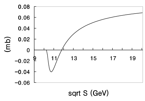
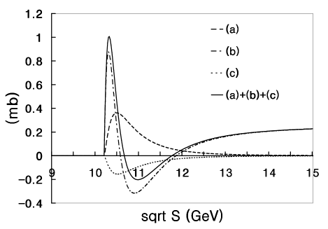
Figure 10: The left figure is the elementary cross section for $\Phi+q\rightarrow Q+\bar{Q}+q$ and the right figure is that for $\Phi+g\rightarrow Q+\bar{Q}+(g)$. In the right figure, (a) the dashed line is the Born term given in Eq. (12). (b) The Dash dotted line is the hard gluon part, namely, the integration of the sum of Eq. (35), Eq. (37), and Eq. (43) over the hard part of the Dalitz plot plus the integration of the ‘$\ln\delta$’ dependent part of Eq. (65) over the soft part of the Dalitz plot. (c) The Dotted line is the soft plus one loop correction, namely, the integration of Eq. (65) excluding the ‘$\ln\delta$’ dependent part over the soft part of the Dalitz plot. The solid line is the sum of (a), (b), and (c).

As an explicit application, the above result is applied to the upsilon dissociation cross section. The two independent parameters of the theory is determined by fitting the physical masses of $m_{\Upsilon(1S)}$ and $m_{\Upsilon(2S)}$ to the energies of the Coulomb bound states. Specifically, from the relation $m_{\Upsilon(2S)}-m_{\Upsilon(1S)}=3/4\epsilon_{o}$, the binding energy is found to be $750MeV$. Also, the bottom quark mass is found to be $5.1\ GeV$ from equating it to $(m_{\Upsilon(1S)}+\epsilon_{o})/2$. The coupling constant $g$ is then found to be $2.53$ from $g^{2}=16\pi/N_{c}\sqrt{\epsilon_{o}/m}$.

The left and right graphs in Fig. (10) represent the elementary total cross sections of $\Phi+q\rightarrow Q+\bar{Q}+q$ and $\Phi+g\rightarrow Q+\bar{Q}+g$ respectively. In both graphs, there are regions of energy where the cross sections become negative. These negative cross sections originate from mass factorization, where finite parts of the differential cross section have been subtracted out and put into the definition of the distribution function. Therefore, the cross section becomes physical only after folding the elementary cross sections with the parton distribution functions (PDF) and adding them to the LO contribution.

To obtain the total cross section, we used the MRST2001LO PDF mrstlo for the LO result, and the MRST2001NLO PDF mrstnlo for the NLO. We used the PDF calculated in the $\overline{MS}$ scheme, because our perturbative calculations, including the subtractions in the mass factorization, were performed in the $\overline{MS}$ scheme. If different schemes were used in the perturbative calculation and in the PDF, the scheme dependent finite pieces would not match, and the result would be inconsistent. In the original scheme of Peskin, the scale of the PDF was be taken to be the binding energy of the system, which is 0.75 GeV in the present system. However, in the present example, we will take it to be $1.25\ GeV^{2}$, which is the minimum $Q^{2}$ scale in the MRST PDF.

The left graph of Fig. (11) shows the total dissociation cross section to LO and to NLO. The ratio between the cross sections calculated to NLO and to LO, plotted in right graph of Fig. (11), shows that perturbative QCD approach is acceptable only in a limited region of energy and large corrections exist in the threshold region.

The separation scale of $1.25\ GeV^{2}$ is low, making it questionable whether one can apply the present formalism to the Upsilon system. On the other hand, one can not take the separation scale to be arbitrarily large in this example, as one would invalidate all the counting schemes and the non relativistic approximations used in deriving the formula. Nevertheless, to asses the uncertainties associated with takin the scale of the PDF to be low, we modified the scale $Q^{2}$ of PDF to $2.0\ GeV^{2}$, and compared the result to that obtained with $Q^{2}=1.25\ GeV^{2}$. As shown in Fig. (12), the total cross section changes by less than 10% for $\sqrt{s}<25GeV$. As shown in the right graph of Fig. (12), $25GeV$ is also the upper limit of the window of energy region where the ratio between NLO to LO is minimal. Hence, although the scale dependence is non negligible in the present example, the uncertainties are within the estimated errors coming from the perturbative expansion.

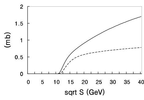
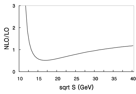
Figure 11: The left figure is the $\Upsilon$(1S)+nucleon total cross section to LO (dashed line) and to NLO (solid line). The right figure is the corresponding ratio between NLO and LO results.

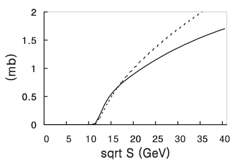
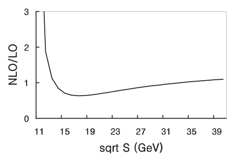
Figure 12: The left figure is the $\Upsilon$(1S)+nucleon total cross section with $Q^{2}=1.25\ GeV^{2}$(straight line) and with $Q^{2}=2.0\ GeV^{2}$(dashed line). The right figure is the ratio between NLO and LO when $Q^{2}=2.0GeV^{2}$.

We also applied the present calculation to the $J/\psi$ dissociation cross section. But in $J/\psi$ case, the soft plus one loop correction has large negative value making the hadronic cross section negative. This suggests that the formalism breaks down for the charmonium system. As the quarkonium is heavier, the relative contribution of this negative part is smaller. Therefore we conclude that charm quark is not heavy enough to use the present formalism in the present form.

VII Conclusion

We have reported on the NLO calculation for the quarkonium parton cross section in QCD. All the collinear divergences have been shown to cancel through mass factorization and the soft divergences among themselves. The result constitutes an exact QCD calculation at the NLO in the formal heavy quark limit.

Explicit application to the Upsilon system shows that there are large NLO corrections especially near the threshold, as has been originally anticipated by Peskinpeskin . Nevertheless, we have identified a window of energy range where the NLO are under control, such that the perturbative QCD results are reliable. Moreover, we have identified the origin of large corrections and assessed the uncertainties through the magnitude of the higher order correction.

The application to the charmonium system confirmed that the discrepancies existing between LO QCD result and hadronic model result on the charmonium dissociation cross section by hadrons especially near threshold are partly due to large higher order corrections in QCD. Nevertheless, since the separation scale is in the order of the binding energy, a thermal mass of few hundred MeV for the partons will be enough to soften the NLO correction and to make a perturbative treatment meaningful at finite temperature.

VIII Acknowledgment

Authors are grateful to W. Beenakker for his kind help, and also to T. Hatsuda, and C. Y. Wong for useful discussion. This work was supported by KOSEF under grant number M02-2004-000-10484-0

Appendix A

Here the phase space of 2-body and 3-body decay are reviewed. The initial flux F is

$$F=4\sqrt{(q\cdot k_{1})^{2}-m_{q}^{2}m_{k_{1}}^{2}}=2\acute{s},$$ (67)

and the total cross section of 2-body decay is

$$\sigma = \frac{\mu^{-D+4}}{2\acute{s}}\int\frac{d^{D}p_{1}}{(2\pi)^{D-1}}\int\frac{d^{D}p_{2}}{(2\pi)^{D-1}}\delta^{+}(p_{1}^{2}-m^{2})\delta^{+}(p_{2}^{2}-m^{2})$$ (68)

$$\times(2\pi)^{D}\delta^{D}(p_{1}+p_{2}-q-k_{1})\overline{|M|^{2}}$$

$$= \frac{\mu^{-D+4}}{2\acute{s}}\int\frac{d^{D}p_{2}}{(2\pi)^{D-2}}\delta^{+}(p_{2}^{2}-m^{2})\delta^{+}((q+k_{1}-p_{2})^{2}-m^{2})\overline{|M|^{2}}.$$

Because

$$\int d^{D}p_{2}\delta^{+}(p_{2}^{2}-m^{2})=\frac{1}{2}\int dp_{20}d|\vec{p_{2}}|^{2}|\vec{p_{2}}|^{D-3}d\Omega_{D-2}\delta^{+}(p_{20}^{2}-|\vec{p_{2}}|^{2}-m^{2})$$

$$=\frac{\pi^{D/2-1}}{\Gamma(D/2-1)}\int dE_{2}d\cos\chi(E_{2}^{2}-m^{2})^{\frac{D-3}{2}}(1-\cos^{2}\chi)^{\frac{D-4}{2}},$$ (69)

where we have used the formula

$$\int^{\pi}_{0}\sin^{D}d\theta=\sqrt{\pi}\frac{\Gamma(D/2+1/2)}{\Gamma(D/2+1)},$$ (70)

and

$$d\Omega_{D-2} = \sin^{D-3}\theta_{1}\sin^{D-4}\theta_{2}...\sin\theta_{D-3}d\theta_{1}d\theta_{2}...d\theta_{D-2}$$ (71)

$$= \frac{2\pi^{D/2-1}}{\Gamma(D/2-1)}\sin^{D-3}\theta_{1}d\theta_{1},$$

the cross section becomes

$$\sigma = \frac{\mu^{-D+4}}{2\acute{s}}\frac{1}{(2\pi)^{D-2}}\frac{\pi^{D/2-1}}{\Gamma(D/2-1)}\int dE_{2}d\cos\chi(E_{2}^{2}-m^{2})^{\frac{D-3}{2}}(1-\cos^{2}\chi)^{\frac{D-4}{2}}$$ (72)

$$\ \ \ \ \ \ \ \ \ \ \ \ \ \ \ \ \ \ \ \ \ \ \ \ \ \ \ \ \ \ \ \ \ \ \ \ \ \ \ \times\delta(s+t_{1}+u_{1})\overline{|M|^{2}},$$

where $(q+k_{1}-p_{2})^{2}-m^{2}=s+t_{1}+u_{1}$.

In the center of mass frame of q and $k_{1}$,

$$q = (E_{q},0,...,0,k_{10})$$

$$k_{1} = (k_{10},0,...,0,-k_{10})$$

$$p_{2} = (E_{2},0,...,|\vec{p}|\sin\chi,|\vec{p}|\cos\chi),$$ (73)

and

$$E_{q} = \frac{s+m_{\Phi}^{2}}{2\sqrt{s}}$$

$$k_{10} = \frac{\acute{s}}{2\sqrt{s}}$$

$$E_{2} = -\frac{t_{1}+u_{1}}{2\sqrt{s}}$$

$$|\vec{p}| = \frac{\sqrt{(t_{1}+u_{1})^{2}-4sm^{2}}}{2\sqrt{s}}$$

$$\cos\chi = \frac{2u_{1}s-(s+m_{\Phi}^{2})(t_{1}+u_{1})}{\acute{s}\sqrt{(t_{1}+u_{1})^{2}-4sm^{2}}}.$$ (74)

From the above relations, the Jacobian from $u_{1},t_{1}$ to $E_{2},\cos\chi$ is

$$dE_{2}d\cos\chi=\frac{\sqrt{s}}{\acute{s}\sqrt{(t_{1}+u_{1})^{2}-4sm^{2}}}dt_{1}du_{1}.$$ (75)

Then the differential cross section is

$$\acute{s}^{2}\frac{d^{2}\sigma}{dt_{1}du_{1}}=\frac{\pi}{\Gamma(D/2-1)}\bigg{(}\frac{1}{4\pi}\bigg{)}^{D/2}\bigg{[}\frac{\acute{s}u_{1}t_{1}-m_{\Phi}^{2}t_{1}^{2}-m^{2}\acute{s}^{2}}{\mu^{2}\acute{s}^{2}}\bigg{]}^{\frac{D-4}{2}}$$

$$\times\delta(s+t_{1}+u_{1})\overline{|M|^{2}}.$$ (76)

Next, the 3-body phase space is

$$\sigma = \frac{\mu^{-2(D-4)}}{2\acute{s}}\int\frac{d^{D}p_{2}}{(2\pi)^{D-1}}\int\frac{d^{D}p_{1}}{(2\pi)^{D-1}}\int\frac{d^{D}k_{2}}{(2\pi)^{D-1}}\delta^{+}(p_{2}^{2}-m^{2})$$ (77)

$$\times\delta^{+}(p_{1}^{2}-m^{2})\delta^{+}(k_{2}^{2})(2\pi)^{D}\delta^{D}(q+k_{1}-p_{1}-p_{2}-k_{2})\bar{|M|}^{2}$$

$$= \frac{1}{2\acute{s}}\frac{\mu^{-2(D-4)}}{(2\pi)^{2D-3}}\int d^{D}p_{2}d^{D}p\delta^{+}(p_{2}^{2}-m^{2})\delta^{D}(q+k_{1}-p_{2}-p)$$

$$\times\int d^{D}k_{2}d^{D}p_{1}\delta^{+}(p_{1}^{2}-m^{2})\delta^{+}(k_{2}^{2})\delta^{D}(p-k_{2}-p_{1})\bar{|M|}^{2}.$$

In the above equation, new variable p is introduced and D-dimensional p integration and D-dimension delta function of p are inserted into phase space. The last line is the same as the two body phase space, and it becomes

$$\frac{-\pi^{\frac{D}{2}}}{2}\frac{\Gamma(\frac{D}{2}-1)}{\Gamma(D-3)}\frac{(p^{2}-m^{2})^{D-3}}{(p^{2})^{\frac{D}{2}-1}}\int^{\pi}_{0}d\theta_{1}\sin^{D-3}\theta_{1}\int^{\pi}_{0}\sin^{D-4}\theta_{2}\bar{|M|}^{2}.$$ (78)

Moving to $q$ and $k_{1}$ center of mass frame, the differential cross section for three body decay is

$$\acute{s}^{2}\frac{d^{2}\sigma}{dt_{1}du_{1}} = \frac{1}{2}\frac{1}{(4\pi)^{D}}\frac{\mu^{-D+4}}{\Gamma(D-3)}\bigg{(}\frac{\acute{s}u_{1}t_{1}-m_{\Phi}^{2}t_{1}^{2}-m^{2}\acute{s}^{2}}{\acute{s}^{2}\mu^{2}}\bigg{)}^{\frac{D-4}{2}}\frac{s_{4}^{D-3}}{(s_{4}+m^{2})^{\frac{D}{2}-1}}$$ (79)

$$\times\int^{\pi}_{0}d\theta_{1}\sin^{D-3}\theta_{1}\int^{\pi}_{0}d\theta_{2}\sin^{D-4}\theta_{2}\overline{|M|}^{2}.$$

Appendix B

Here the angular integration which are used throughout this work is derived. The required angular integration has the form

$$I_{D}^{(i,j)} \equiv \int^{\pi}_{0}d\theta_{1}\sin^{D-3}\theta_{1}\int^{\pi}_{0}d\theta_{2}\sin^{D-4}\theta_{2}\frac{1}{\acute{t}^{i}(\acute{u}+\acute{s})^{j}}$$ (80)

$$= \int^{\pi}_{0}d\theta_{1}\int^{\pi}_{0}d\theta_{2}\frac{\sin^{D-3}\theta_{1}\sin^{D-4}\theta_{2}}{(a+b\cos\theta_{1})^{i}(A+B\cos\theta_{1}+C\sin\theta_{1}\cos\theta_{2})^{j}},$$

where

$$A = 2E_{q}(k_{10}-k_{20})+2k_{10}(k_{10}-|\vec{p}|\cos\varphi)$$

$$B = 2k_{20}(|\vec{p}|\cos\varphi-k_{10})$$

$$C = 2k_{20}|\vec{p}|\sin\varphi$$

$$a = -2k_{10}k_{20}.$$ (81)

D denote that it is D-dimensional angular integration. If $b=-a,A^{2}=B^{2}+C^{2}$, the solution has an explicit form Beenakker neerven .

$$I_{D}^{(i,j)}=\frac{2\pi}{(2a)^{i}(2A)^{j}}\frac{\Gamma(D/2-i-1)\Gamma(D/2-j-1)\Gamma(D-3)}{\Gamma^{2}(D/2-1)\Gamma(D-i-j-2)}$$

$$\times F_{1,2}\bigg{[}i,j,\frac{D}{2}-1;\frac{A-B}{2A}\bigg{]}.$$ (82)

$F_{1,2}$ is the hypergeometric function.

$$F_{1,2}(a,b,c;x)\equiv\frac{\Gamma(c)}{\Gamma(b)\Gamma(c-b)}\int^{1}_{0}dt\ t^{b-1}(1-t)^{c-b-1}(1-tx)^{-a},$$ (83)

which has the following properties

$$F_{1,2}(a,b,c;x) = F_{1,2}(b,a,c;x)$$

$$F_{1,2}(0,b,c;x) = 1.$$ (84)

In the present case $b=-a$, and $A^{2}\neq B^{2}+C^{2}$. First, considering $I_{D}^{(1,1)}$,

$$I_{D}^{(1,1)} = \int^{\pi}_{0}d\theta_{1}\int^{\pi}_{0}d\theta_{2}\frac{\sin^{D-3}\theta_{1}\sin^{D-4}\theta_{2}}{a(1-\cos\theta_{1})(A+B\cos\theta_{1}+C\sin\theta_{1}\cos\theta_{2})}$$ (85)

$$= \frac{1}{a(A+B)}\int^{\pi}_{0}d\theta_{1}\int^{\pi}_{0}d\theta_{2}\frac{\sin^{D-3}\theta_{1}\sin^{D-4}\theta_{2}}{(1-\cos\theta_{1})}$$

$$-\frac{1}{a(A+B)}\int^{\pi}_{0}d\theta_{1}\int^{\pi}_{0}d\theta_{2}\frac{\sin^{D-3}\theta_{1}\sin^{D-4}\theta_{2}}{(1-\cos\theta_{1})}$$

$$\ \ \ \ \ \ \ \ \ \ \ \ \ \times\bigg{[}1-\frac{A+B}{A+B\cos\theta_{1}+C\sin\theta_{1}\cos\theta_{2}}\bigg{]}$$

$$\equiv I_{1}+I_{2},$$

where $I$ is separated into infinite part $I_{1}$ and finite part $I_{2}$ in $4$ dimension.

From Eq. (82)

$$I_{1}=\frac{I_{D}^{(1,0)}}{A+B}=\frac{\pi}{a(A+B)}\frac{2}{D-4},$$ (86)

and

$$I_{2} \approx -\frac{1}{a(A+B)}\int^{1}_{-1}d\cos\theta_{1}\int^{\pi}_{0}d\theta_{2}\frac{1}{(1-\cos\theta_{1})}$$ (87)

$$\times\bigg{[}1-\frac{A+B}{A+B\cos\theta_{1}+C\sin\theta_{1}\cos\theta_{2}}\bigg{]}+\Theta(D-4)$$

$$= -\frac{\pi}{a(A+B)}\int^{1}_{-1}\frac{d\cos\theta_{1}}{1-\cos\theta_{1}}$$

$$\times\bigg{[}1-\frac{A+B}{\sqrt{(A+B\cos\theta_{1})^{2}-C^{2}\sin^{2}\theta_{1}}}\bigg{]}+\Theta(D-4)$$

$$= \frac{\pi}{a(A+B)}\ln\bigg{[}(A+B)^{2}-(1-\cos\theta_{1})(B^{2}+C^{2}+AB)$$

$$+(A+B)\sqrt{(A+B\cos\theta_{1})^{2}+C^{2}\sin^{2}\theta_{1}}\bigg{]}\bigg{|}^{\cos\theta_{1}=+1}_{\cos\theta_{1}=-1}+\Theta(D-4)$$

$$= \frac{\pi}{a(A+B)}\ln\frac{(A+B)^{2}}{A^{2}-B^{2}-C^{2}}+\Theta(D-4).$$

As a result,

$$I_{D}^{(1,1)}=\frac{\pi}{a(A+B)}\bigg{[}\frac{2}{D-4}+\ln\frac{(A+B)^{2}}{A^{2}-B^{2}-C^{2}}\bigg{]}+\Theta(D-4).$$ (88)

$I_{D}^{(1,j)}$ with higher order $j$ is derived by differentiating $I_{D}^{(1,1)}$ with respect to $A$.

$$I_{D}^{(1,j)}=\frac{(-1)^{j-1}}{(j-1)!}\frac{d^{j-1}}{dA^{j-1}}I_{D}^{(1,1)}.$$ (89)

Below are the summary of the results. (the subscript ‘D’ is omitted for simplicity).

$$I^{(1,0)}=\frac{2\pi}{a}\frac{1}{D-4}$$ (90)

$$I^{(1,1)} = \frac{\pi}{a(A+B)}\bigg{(}\frac{2}{D-4}+\ln\bigg{[}\frac{(A+B)^{2}}{A^{2}-B^{2}-C^{2}}\bigg{]}$$ (91)

$$+\frac{D-4}{2}\bigg{[}\ln^{2}\frac{A-\sqrt{B^{2}+C^{2}}}{A+B}-\frac{1}{2}\ln^{2}\frac{A+\sqrt{B^{2}+C^{2}}}{A-\sqrt{B^{2}+C^{2}}}$$

$$+2Li_{2}\bigg{(}-\frac{B+\sqrt{B^{2}+C^{2}}}{A-\sqrt{B^{2}+C^{2}}}\bigg{)}-2Li_{2}\bigg{(}\frac{A-\sqrt{B^{2}+C^{2}}}{A+B}\bigg{)}\bigg{]}$$

$$+O((D-4)^{2})\bigg{)}$$

$$I^{(1,2)}=\frac{\pi}{a(A+B)^{2}}\bigg{(}\frac{2}{D-4}+\ln\bigg{[}\frac{(A+B)^{2}}{A^{2}-B^{2}-C^{2}}\bigg{]}+O(D-4)\bigg{)}$$ (92)

$$I^{(1,3)}=\frac{\pi}{a(A+B)^{3}}\bigg{(}\frac{2}{D-4}+\ln\bigg{[}\frac{(A+B)^{2}}{A^{2}-B^{2}-C^{2}}\bigg{]}+\frac{2A(A+B)}{A^{2}-B^{2}-C^{2}}$$

$$+(A+B)^{2}\frac{A^{2}+B^{2}+C^{2}}{(A^{2}-B^{2}-C^{2})^{2}}-3+O(D-4)\bigg{)}$$ (93)

$$I^{(1,4)} = \frac{\pi}{a(A+B)^{4}}\bigg{(}\frac{2}{D-4}+\ln\bigg{[}\frac{(A+B)^{2}}{A^{2}-B^{2}-C^{2}}\bigg{]}+\frac{2A(A+B)}{A^{2}-B^{2}-C^{2}}$$ (94)

$$+(A+B)^{2}\frac{A^{2}+B^{2}+C^{2}}{(A^{2}-B^{2}-C^{2})^{2}}+(A+B)^{3}\frac{2A^{3}+6AB^{2}+6AC^{2}}{3(A^{2}-B^{2}-C^{2})^{3}}$$

$$-11/3+O(D-4)\bigg{)}$$

$$I^{(1,5)} = \frac{\pi}{a(A+B)^{5}}\bigg{(}\frac{2}{D-4}+\ln\bigg{[}\frac{(A+B)^{2}}{A^{2}-B^{2}-C^{2}}\bigg{]}+\frac{2A(A+B)}{A^{2}-B^{2}-C^{2}}$$ (95)

$$+(A+B)^{2}\frac{A^{2}+B^{2}+C^{2}}{(A^{2}-B^{2}-C^{2})^{2}}+(A+B)^{3}\frac{2A(A^{2}+3B^{2}+3C^{2})}{3(A^{2}-B^{2}-C^{2})^{3}}$$

$$+(A+B)^{4}\bigg{[}\frac{4A^{2}(B^{2}+C^{2})}{(A^{2}-B^{2}-C^{2})^{4}}+\frac{1}{(A^{2}-B^{2}-C^{2})^{2}}\bigg{]}$$

$$-25/4+O(D-4)\bigg{)}$$

$$I^{(1,6)} = \frac{\pi}{a(A+B)^{6}}\bigg{(}\frac{2}{D-4}+\ln\bigg{[}\frac{(A+B)^{2}}{A^{2}-B^{2}-C^{2}}\bigg{]}+\frac{2A(A+B)}{A^{2}-B^{2}-C^{2}}$$ (96)

$$+(A+B)^{2}\frac{A^{2}+B^{2}+C^{2}}{(A^{2}-B^{2}-C^{2})^{2}}+(A+B)^{3}\frac{2A(A^{2}+3B^{2}+3C^{2})}{3(A^{2}-B^{2}-C^{2})^{3}}$$

$$+(A+B)^{4}\bigg{[}\frac{4A^{2}(B^{2}+C^{2})}{(A^{2}-B^{2}-C^{2})^{4}}+\frac{1}{(A^{2}-B^{2}-C^{2})^{2}}\bigg{]}$$

$$+(A+B)^{5}\bigg{[}\frac{32A^{5}}{5(A^{2}-B^{2}-C^{2})^{5}}-\frac{2A(3A^{2}+B^{2}+C^{2})}{(A^{2}-B^{2}-C^{2})^{4}}\bigg{]}$$

$$-137/30+O(D-4)\bigg{)}$$

$I^{(0,j)}$ and $I^{(-1,j)}$ may be obtained from Beenakker and by the same method,

$$I^{(0,1)}=\frac{\pi\ln\bigg{(}\frac{A+\sqrt{B^{2}+C^{2}}}{A-\sqrt{B^{2}+C^{2}}}\bigg{)}}{\sqrt{B^{2}+C^{2}}}$$ (97)

$$I^{(0,2)}=\frac{2\pi}{A^{2}-B^{2}-C^{2}}$$ (98)

$$I^{(0,3)}=\frac{2\pi A}{(A^{2}-B^{2}-C^{2})^{2}}$$ (99)

$$I^{(0,4)}=-\frac{2\pi(3A^{2}+B^{2}+C^{2})}{3(A^{2}-B^{2}-C^{2})^{3}}$$ (100)

$$I^{(0,5)}=\frac{2\pi A(A^{2}+B^{2}+C^{2})}{(A^{2}-B^{2}-C^{2})^{4}}$$ (101)

$$I^{(0,6)}=\frac{2\pi(5A^{2}+10A^{2}(B^{2}+C^{2})+(B^{2}+C^{2})^{2})}{5(A^{2}-B^{2}-C^{2})^{5}}$$ (102)

$$I^{(-1,1)}=\pi a\bigg{(}-\frac{2B}{B^{2}+C^{2}}+\frac{B^{2}+C^{2}+AB}{(B^{2}+C^{2})^{3/2}}\ln\bigg{[}\frac{A+\sqrt{B^{2}+C^{2}}}{A-\sqrt{B^{2}+C^{2}}}\bigg{]}\bigg{)}$$ (103)

$$I^{(-1,2)} = \pi a\bigg{(}\frac{2(AB+B^{2}+C^{2})}{(B^{2}+C^{2})(A^{2}-B^{2}-C^{2})}$$ (104)

$$-\frac{B}{(B^{2}+C^{2})^{3/2}}\ln\bigg{[}\frac{A+\sqrt{B^{2}+C^{2}}}{A-\sqrt{B^{2}+C^{2}}}\bigg{]}\bigg{)}$$

$$I^{(-1,3)}=\frac{2\pi a(A+B)}{(A^{2}-B^{2}-C^{2})^{2}}$$ (105)

$$I^{(-1,4)}=\frac{2\pi a(3A^{2}+4AB+B^{2}+C^{2})}{3(A^{2}-B^{2}-C^{2})^{3}}$$ (106)

$$I^{(-1,5)}=\frac{2\pi a(3A^{3}+5A^{2}B+(3A+B)(B^{2}+C^{2}))}{3(A^{2}-B^{2}-C^{2})^{4}}$$ (107)

$$I^{(-1,6)}=$$

$$\frac{2\pi a(5A^{4}+10A^{3}B+(10A^{2}+6AB)(B^{2}+C^{2})+(B^{2}+C^{2})^{2})}{5(A^{2}-B^{2}-C^{2})^{5}}.$$ (108)

Appendix C

Here the detail calculation of Fig. (6) is presented. $M_{1}$ through $M_{8}$ correspond to tree diagrams (1) to (8).

$M_{1}$ is

$$M_{\mu\nu\lambda}^{(1)} = (ig)^{2}\bar{u}(p_{1})\Gamma_{\mu}(p_{1},p_{1}-q)i\Delta(p_{1}-q)\gamma_{\nu}T^{a}$$ (109)

$$\ \ \ \ \ \ \times i\Delta(-p_{2}-k_{2})\gamma_{\lambda}T^{b}v(p_{2})$$

$$= g^{2}\sqrt{\frac{m_{\Phi}}{N_{c}}}\bar{u}(p_{1})\frac{1+\gamma^{0}}{2}\gamma_{i}g^{i\mu}\frac{1-\gamma^{0}}{2}T^{a}T^{b}v(p_{2})$$

$$\times\psi(p)\bigg{[}g^{0}_{\nu}g^{0}_{\lambda}\frac{-1}{k_{20}}$$

$$\ \ \ \ \ \ \ \ \ \ \ \ -g^{0}_{\nu}g^{0}_{\lambda}\frac{\vec{p_{2}}\cdot\vec{k_{2}}}{mk_{20}^{2}}-g^{0}_{\nu}\frac{p_{2j}g^{j}_{\lambda}}{mk_{20}}+g^{0}_{\lambda}\frac{p_{1j}g^{j}_{\nu}}{mk_{20}}\bigg{]}.$$

The first line in the bracket is of $1/(mg^{4})$ order, and the second line is of $1/(mg^{2})$ order from Eq. (9). As will be shown later, the sum of $1/(mg^{4})$ order terms from $M_{1}$ to $M_{8}$ vanishes. As a result, the $1/(mg^{2})$ order becomes the leading order.

$M_{2}$ is

$$M_{\mu\nu\lambda}^{(2)} = (ig)^{2}\bar{u}(p_{1})\gamma_{\lambda}T^{b}i\Delta(p_{1}+k_{2})\gamma_{\nu}T^{a}i\Delta(q-p_{2})$$ (110)

$$\ \ \ \ \ \ \times\Gamma_{\mu}(-p_{2},q-p_{2})v(p_{2})$$

$$= g^{2}\sqrt{\frac{m_{\Phi}}{N_{c}}}\bar{u}(p_{1})\frac{1+\gamma^{0}}{2}\gamma_{i}g^{i\mu}\frac{1-\gamma^{0}}{2}T^{b}T^{a}v(p_{2})$$

$$\times\bigg{[}g_{\nu}^{0}g_{\lambda}^{0}\frac{-1}{k_{20}}\psi(p)$$

$$\ \ \ \ \ \ \ \ \ \ \ \ +\bigg{(}g_{\nu}^{j}g_{\lambda}^{0}\frac{p_{2j}}{mk_{20}}-g_{\nu}^{0}g_{\lambda}^{j}\frac{p_{1j}}{mk_{20}}-g_{\nu}^{0}g_{\lambda}^{0}\frac{\vec{p_{1}}\cdot\vec{k_{2}}}{mk_{20}^{2}}\bigg{)}\psi(p)$$

$$\ \ \ \ \ \ \ \ \ \ \ \ +g_{\nu}^{0}g_{\lambda}^{0}\frac{-1}{k_{20}}\frac{\partial\psi(p)}{\partial\vec{p}}\cdot(-\vec{k_{1}}+\vec{k_{2}})\bigg{]}.$$

The third line in the bracket comes from the expansion of the Bethe-Salpeter amplitude.

$$\Gamma_{\mu}(p_{1}+k_{2},-p_{2}+k_{1}) = \Gamma_{\mu}(\vec{p_{1}}+\vec{k_{2}},\vec{p_{1}}+\vec{k_{2}})$$ (111)

$$= \Gamma_{\mu}(\vec{p_{1}},\vec{p_{1}})+\frac{\partial\Gamma_{\mu}(\vec{p_{1}},\vec{p_{1}})}{\partial\vec{p}}\cdot\vec{k_{2}}$$

$$\Gamma_{\mu}(-p_{2},q-p_{2}) = \Gamma_{\mu}(\vec{p_{1}}-\vec{k_{1}}+\vec{k_{2}},\vec{p_{1}}-\vec{k_{1}}+\vec{k_{2}})$$ (112)

$$= \Gamma_{\mu}(\vec{p_{1}},\vec{p_{1}})+\frac{\partial\Gamma_{\mu}(\vec{p_{1}},\vec{p_{1}})}{\partial\vec{p}}\cdot(-\vec{k_{1}}+\vec{k_{2}})$$

$$\Gamma_{\mu}(p_{1}-k_{1},-p_{2}-k_{2}) = \Gamma_{\mu}(\vec{p_{1}}-\vec{k_{1}},\vec{p_{1}}-\vec{k_{1}})$$ (113)

$$= \Gamma_{\mu}(\vec{p_{1}},\vec{p_{1}})+\frac{\partial\Gamma_{\mu}(\vec{p_{1}},\vec{p_{1}})}{\partial\vec{p}}\cdot(-\vec{k_{1}}).$$

$M^{3}$ is

$$M_{\mu\nu\lambda}^{(3)} = (ig)^{2}\bar{u}(p_{1})\gamma_{\lambda}T^{b}i\Delta(p_{1}+k_{2})\Gamma_{\mu}(p_{1}+k_{2},-p_{2}+k_{1})$$

$$\ \ \ \ \ \ \times i\Delta(-p_{2}+k_{1})\gamma_{\nu}T^{a}v(p_{2})$$

$$= g^{2}\sqrt{\frac{m_{\Phi}}{N_{c}}}\bar{u}(p_{1})\frac{1+\gamma^{0}}{2}\gamma_{i}g^{i\mu}\frac{1-\gamma^{0}}{2}T^{b}T^{a}v(p_{2})$$

$$\times\bigg{[}g^{0}_{\nu}g^{0}_{\lambda}\frac{-\epsilon+|\vec{p_{1}}|^{2}/m}{k_{10}k_{20}}\psi(p)$$

$$\ \ \ \ \ \ +g^{0}_{\nu}g^{0}_{\lambda}\bigg{(}-\frac{\vec{p_{2}}\cdot\vec{k_{1}}}{mk_{10}^{2}}+\frac{\vec{p_{2}}\cdot\vec{k_{1}}-\vec{p_{1}}\cdot\vec{k_{2}}}{mk_{10}k_{20}}+\frac{\vec{p_{1}}\cdot\vec{k_{2}}}{mk_{20}^{2}}\bigg{)}\psi(p)$$

$$\ \ \ \ \ \ +\bigg{(}g^{j}_{\nu}g^{0}_{\lambda}\frac{p_{2j}}{m}\frac{k_{10}-k_{20}}{k_{10}k_{20}}+g^{0}_{\nu}g^{j}_{\lambda}\frac{p_{1j}}{m}\frac{k_{10}-k_{20}}{k_{10}k_{20}}\bigg{)}\psi(p)$$

$$\ \ \ \ \ \ +g^{0}_{\nu}g^{0}_{\lambda}\bigg{(}\frac{2\vec{p_{1}}\cdot\vec{k_{2}}}{mk_{10}k_{20}}\psi(p)+\frac{k_{10}-k_{20}}{k_{10}k_{20}}\frac{\partial\psi(p)}{\partial\vec{p}}\cdot\vec{k_{2}}\bigg{)}\bigg{]}$$

$$= g^{2}\sqrt{\frac{m_{\Phi}}{N_{c}}}\bar{u}(p_{1})\frac{1+\gamma^{0}}{2}\gamma_{i}g^{i\mu}\frac{1-\gamma^{0}}{2}T^{b}T^{a}v(p_{2})$$

$$\times\bigg{[}g^{0}_{\nu}g^{0}_{\lambda}\frac{k_{10}-k_{20}}{k_{10}k_{20}}\psi(p)$$

$$\ \ \ \ \ \ +g^{0}_{\nu}g^{0}_{\lambda}\bigg{(}-\frac{\vec{p_{2}}\cdot\vec{k_{1}}}{mk_{10}^{2}}+\frac{\vec{p_{2}}\cdot\vec{k_{1}}-\vec{p_{1}}\cdot\vec{k_{2}}}{mk_{10}k_{20}}+\frac{\vec{p_{1}}\cdot\vec{k_{2}}}{mk_{20}^{2}}\bigg{)}\psi(p)$$

$$\ \ \ \ \ \ +\bigg{(}g^{j}_{\nu}g^{0}_{\lambda}\frac{p_{2j}}{m}\frac{k_{10}-k_{20}}{k_{10}k_{20}}+g^{0}_{\nu}g^{j}_{\lambda}\frac{p_{1j}}{m}\frac{k_{10}-k_{20}}{k_{10}k_{20}}\bigg{)}\psi(p)$$

$$\ \ \ \ \ \ +g^{0}_{\nu}g^{0}_{\lambda}\bigg{(}\frac{\vec{p_{1}}\cdot\vec{k_{1}}+\vec{p_{1}}\cdot\vec{k_{2}}}{mk_{10}k_{20}}\psi(p)+\frac{k_{10}-k_{20}}{k_{10}k_{20}}\frac{\partial\psi(p)}{\partial\vec{p}}\cdot\vec{k_{2}}\bigg{)}\bigg{]},$$

Notice that $|\vec{p_{2}}|^{2}\approx|\vec{p_{1}}|^{2}-2\vec{p_{1}}\cdot(\vec{k_{1}}-\vec{k_{2}})$ from the order counting of Eq. (9). The last line in the last equation comes from the expansion of the Bethe-Salpeter amplitude in Eq. (111).

Similarly, $M^{4}$ to $M^{8}$ are given as below.

$$M_{\mu\nu\lambda}^{(4)} = (ig)^{2}\bar{u}(p_{1})\gamma_{\nu}T^{a}i\Delta(p_{1}-k_{1})\Gamma_{\mu}(p_{1}-k_{1},-p_{2}-k_{2})$$

$$\ \ \ \ \ \ \times i\Delta(-p_{2}-k_{2})\gamma_{\lambda}T^{b}v(p_{2})$$

$$= g^{2}\sqrt{\frac{m_{\Phi}}{N_{c}}}\bar{u}(p_{1})\frac{1+\gamma^{0}}{2}\gamma_{i}g^{i\mu}\frac{1-\gamma^{0}}{2}T^{a}T^{b}v(p_{2})$$

$$\times\bigg{[}g^{0}_{\nu}g^{0}_{\lambda}\frac{-\epsilon+|\vec{p_{1}}|^{2}/m}{k_{10}k_{20}}\psi(p)$$

$$\ \ \ \ \ \ +g^{0}_{\nu}g^{0}_{\lambda}\bigg{(}-\frac{\vec{p_{1}}\cdot\vec{k_{1}}}{mk_{10}^{2}}+\frac{\vec{p_{1}}\cdot\vec{k_{1}}-\vec{p_{2}}\cdot\vec{k_{2}}}{mk_{10}k_{20}}+\frac{\vec{p_{2}}\cdot\vec{k_{2}}}{mk_{20}^{2}}\bigg{)}\psi(p)$$

$$\ \ \ \ \ \ +\bigg{(}g^{j}_{\nu}g^{0}_{\lambda}\frac{p_{1j}}{m}\frac{k_{10}-k_{20}}{k_{10}k_{20}}+g^{0}_{\nu}g^{j}_{\lambda}\frac{p_{2j}}{m}\frac{k_{10}-k_{20}}{k_{10}k_{20}}\bigg{)}\psi(p)$$

$$\ \ \ \ \ \ +g^{0}_{\nu}g^{0}_{\lambda}\bigg{(}-\frac{2\vec{p_{1}}\cdot\vec{k_{1}}}{mk_{10}k_{20}}\psi(p)+\frac{k_{10}-k_{20}}{k_{10}k_{20}}\frac{\partial\psi(p)}{\partial\vec{p}}\cdot(-\vec{k_{1}})\bigg{)}\bigg{]}$$

$$= g^{2}\sqrt{\frac{m_{\Phi}}{N_{c}}}\bar{u}(p_{1})\frac{1+\gamma^{0}}{2}\gamma_{i}g^{i\mu}\frac{1-\gamma^{0}}{2}T^{b}T^{a}v(p_{2})$$

$$\times\bigg{[}g^{0}_{\nu}g^{0}_{\lambda}\frac{k_{10}-k_{20}}{k_{10}k_{20}}\psi(p)$$

$$\ \ \ \ \ \ +g^{0}_{\nu}g^{0}_{\lambda}\bigg{(}-\frac{\vec{p_{1}}\cdot\vec{k_{1}}}{mk_{10}^{2}}+\frac{\vec{p_{1}}\cdot\vec{k_{1}}-\vec{p_{2}}\cdot\vec{k_{2}}}{mk_{10}k_{20}}+\frac{\vec{p_{2}}\cdot\vec{k_{2}}}{mk_{20}^{2}}\bigg{)}\psi(p)$$

$$\ \ \ \ \ \ +\bigg{(}g^{j}_{\nu}g^{0}_{\lambda}\frac{p_{1j}}{m}\frac{k_{10}-k_{20}}{k_{10}k_{20}}+g^{0}_{\nu}g^{j}_{\lambda}\frac{p_{2j}}{m}\frac{k_{10}-k_{20}}{k_{10}k_{20}}\bigg{)}\psi(p)$$

$$\ \ \ \ \ \ -g^{0}_{\nu}g^{0}_{\lambda}\bigg{(}\frac{\vec{p_{1}}\cdot\vec{k_{2}}+\vec{p_{1}}\cdot\vec{k_{1}}}{mk_{10}k_{20}}\psi(p)+\frac{k_{10}-k_{20}}{k_{10}k_{20}}\frac{\partial\psi(p)}{\partial\vec{p}}\cdot\vec{k_{1}}\bigg{)}\bigg{]}$$

$$M_{\mu\nu\lambda}^{(5)} = (ig)^{2}\bar{u}(p_{1})\Gamma_{\mu}(p_{1},p_{1}-q)i\Delta(p_{1}-q)\gamma_{\lambda}T^{b}$$ (116)

$$\ \ \ \ \ \ \times i\Delta(-p_{2}+k_{1})\gamma_{\nu}T^{a}v(p_{2})$$

$$= g^{2}\sqrt{\frac{m_{\Phi}}{N_{c}}}\bar{u}(p_{1})\frac{1+\gamma^{0}}{2}\gamma_{i}g^{i\mu}\frac{1-\gamma^{0}}{2}T^{b}T^{a}v(p_{2})$$

$$\times\psi(p)\bigg{[}g^{0}_{\nu}g^{0}_{\lambda}\frac{1}{k_{10}}$$

$$\ \ \ \ \ \ \ \ \ \ \ \ +g^{0}_{\nu}g^{0}_{\lambda}\frac{\vec{p_{2}}\cdot\vec{k_{1}}}{mk_{10}^{2}}-g^{0}_{\nu}\frac{p_{1j}g^{j}_{\lambda}}{mk_{10}}+g^{0}_{\lambda}\frac{p_{2j}g^{j}_{\nu}}{mk_{10}}\bigg{]}$$

$$M_{\mu\nu\lambda}^{(6)} = (ig)^{2}\bar{u}(p_{1})\gamma_{\nu}T^{a}i\Delta(p_{1}-k_{1})\gamma_{\lambda}T^{b}i\Delta(q-p_{2})$$ (117)

$$\ \ \ \ \ \ \times\Gamma_{\mu}(q-p_{2},-p_{2})v(p_{2})$$

$$= g^{2}\sqrt{\frac{m_{\Phi}}{N_{c}}}\bar{u}(p_{1})\frac{1+\gamma^{0}}{2}\gamma_{i}g^{i\mu}\frac{1-\gamma^{0}}{2}T^{b}T^{a}v(p_{2})$$

$$\times\bigg{[}g_{\nu}^{0}g_{\lambda}^{0}\frac{1}{k_{10}}\psi(p)$$

$$\ \ \ \ \ \ \ \ \ \ \ \ +\bigg{(}g_{\nu}^{j}g_{\lambda}^{0}\frac{p_{1j}}{mk_{10}}-g_{\nu}^{0}g_{\lambda}^{j}\frac{p_{2j}}{mk_{10}}+g_{\nu}^{0}g_{\lambda}^{0}\frac{\vec{p_{1}}\cdot\vec{k_{1}}}{mk_{10}^{2}}\bigg{)}\psi(p)$$

$$\ \ \ \ \ \ \ \ \ \ \ \ +g_{\nu}^{0}g_{\lambda}^{0}\frac{1}{k_{10}}\frac{\partial\psi(p)}{\partial\vec{p}}\cdot(-\vec{k_{1}}+\vec{k_{2}})\bigg{]}$$

$$M_{\mu\nu\lambda}^{(7)} = ig\bar{u}(p_{1})\Gamma_{\mu}(p_{1},p_{1}-q)i\Delta(p_{1}-q)\gamma^{\delta}T^{c}v(p_{2})\frac{-i}{(k_{1}-k_{2})^{2}}$$ (118)

$$\times gf_{abc}\bigg{(}(k_{1}+k_{2})_{\delta}g_{\nu\lambda}+(-2k_{2}+k_{1})_{\nu}g_{\lambda\delta}+(-2k_{1}+k_{2})_{\lambda}g_{\nu\delta}\bigg{)}$$

$$= g^{2}\sqrt{\frac{m_{\Phi}}{N_{c}}}\bar{u}(p_{1})\frac{1+\gamma^{0}}{2}\gamma_{i}g^{i\mu}\frac{1-\gamma^{0}}{2}[T^{a},T^{b}]v(p_{2})\frac{1}{(k_{1}-k_{2})^{2}}$$

$$\times\bigg{[}(k_{1}+k_{2})_{0}g_{\nu\lambda}+(-2k_{2}+k_{1})_{\nu}g_{\lambda 0}+(-2k_{1}+k_{2})_{\lambda}g_{\nu 0}$$

$$\ \ \ \ \ \ \frac{\vec{p_{1}}\cdot\vec{k_{1}}+\vec{p_{1}}\cdot\vec{k_{2}}}{m}g_{\nu\lambda}+\frac{2k_{1j}p_{1k}+2k_{1k}p_{1j}}{m}g_{\nu}^{j}g_{\lambda}^{k}\bigg{]}\psi(p)$$

$$M_{\mu\nu\lambda}^{(8)} = ig\bar{u}(p_{1})\gamma^{\delta}T^{c}i\Delta(q-p_{2})\Gamma_{\mu}(q-p_{2},-p_{2})v(p_{2})\frac{-i}{(k_{1}-k_{2})^{2}}$$ (119)

$$\times gf_{abc}\bigg{(}(k_{1}+k_{2})_{\delta}g_{\nu\lambda}+(-2k_{2}+k_{1})_{\nu}g_{\lambda\delta}+(-2k_{1}+k_{2})_{\lambda}g_{\nu\delta}\bigg{)}$$

$$= g^{2}\sqrt{\frac{m_{\Phi}}{N_{c}}}\bar{u}(p_{1})\frac{1+\gamma^{0}}{2}\gamma_{i}g^{i\mu}\frac{1-\gamma^{0}}{2}[T^{a},T^{b}]v(p_{2})\frac{1}{(k_{1}-k_{2})^{2}}$$

$$\times\bigg{[}-\bigg{(}(k_{1}+k_{2})_{0}g_{\nu\lambda}+(-2k_{2}+k_{1})_{\nu}g_{\lambda 0}+(-2k_{1}+k_{2})_{\lambda}g_{\nu 0}$$

$$\ \ \ \ \ \ \ \ \ \ \ \ \frac{\vec{p_{2}}\cdot\vec{k_{1}}+\vec{p_{2}}\cdot\vec{k_{2}}}{m}g_{\nu\lambda}+\frac{2k_{1j}p_{2k}+2k_{1k}p_{2j}}{m}g_{\nu}^{j}g_{\lambda}^{k}\bigg{)}\psi(p)$$

$$\ \ \ \ \ \ +\bigg{(}(k_{1}+k_{2})_{0}g_{\nu\lambda}+(-2k_{2}+k_{1})_{\nu}g_{\lambda 0}+(-2k_{1}+k_{2})_{\lambda}g_{\nu 0}\bigg{)}$$

$$\ \ \ \ \ \ \ \ \ \ \ \ \times\frac{\partial\psi(p)}{\partial\vec{p}}\cdot(\vec{k_{1}}-\vec{k_{2}})\ \ \ \bigg{]}.$$

Next considering others,

$$M_{\mu\nu\lambda}^{(9)} = (ig)^{3}\int\frac{d^{4}k}{(2\pi)^{4}}\gamma_{\lambda}T^{b}i\Delta(p_{1}+k_{2})\gamma^{\sigma}T^{c}i\Delta(k+q)\Gamma_{\mu}(k+q,k)$$ (120)

$$\times i\Delta(k)\gamma^{\delta}T^{d}v(p_{2})\frac{-i}{(k+p_{2})^{2}}\frac{-i}{(k+p_{2}-k_{1})^{2}}$$

$$\times gf^{cad}\bigg{(}(k+p_{2}-2k_{1})_{\delta}g_{\sigma\nu}+(k_{1}+k+p_{2})_{\sigma}g_{\nu\delta}+(-2k-2p_{2}+k_{1})_{\nu}g_{\sigma\delta}\bigg{)}$$

$$= g^{2}\sqrt{\frac{m_{\Phi}}{N_{c}}}\bar{u}(p_{1})\frac{1+\gamma^{0}}{2}\gamma_{i}g^{i\mu}\frac{1-\gamma^{0}}{2}T^{b}T^{a}v(p_{2})$$

$$\times g_{\nu}^{j}g_{\lambda}^{0}\frac{1}{k_{20}}\bigg{[}\ \frac{2p_{1j}}{m}\psi(p)-\bigg{(}\epsilon-\frac{|\vec{p}|^{2}}{m}\bigg{)}\frac{\partial\psi(p)}{\partial p_{j}}\ \bigg{]}$$

$$M_{\mu\nu\lambda}^{(10)} = (ig)^{3}\int\frac{d^{4}k}{(2\pi)^{4}}\gamma^{\sigma}T^{c}i\Delta(k)\Gamma_{\mu}(k,k-q)i\Delta(k-q)\gamma^{\delta}T^{d}$$ (121)

$$\times i\Delta(-p_{2}-k_{2})\gamma_{\lambda}T^{b}v(p_{2})\frac{-i}{(k-p_{1})^{2}}\frac{-i}{(k-p_{1}+k_{1})^{2}}$$

$$\times gf^{cad}\bigg{(}(k-p_{1}-k_{1})_{\delta}g_{\sigma\nu}+(2k_{1}+k-p_{1})_{\sigma}g_{\nu\delta}+(-2k+2p_{1}-k_{1})_{\nu}g_{\sigma\delta}\bigg{)}$$

$$= g^{2}\sqrt{\frac{m_{\Phi}}{N_{c}}}\bar{u}(p_{1})\frac{1+\gamma^{0}}{2}\gamma_{i}g^{i\mu}\frac{1-\gamma^{0}}{2}T^{a}T^{b}v(p_{2})$$

$$\times g_{\nu}^{j}g_{\lambda}^{0}\frac{1}{k_{20}}\bigg{[}\ -\frac{2p_{1j}}{m}\psi(p)+\bigg{(}\epsilon-\frac{|\vec{p}|^{2}}{m}\bigg{)}\frac{\partial\psi(p)}{\partial p_{j}}\ \bigg{]}$$

$$M_{\mu\nu\lambda}^{(11)} = (ig)^{3}\int\frac{d^{4}k}{(2\pi)^{4}}\gamma_{\nu}T^{a}i\Delta(p_{1}-k_{1})\gamma^{\sigma}T^{c}i\Delta(k+q)\Gamma_{\mu}(k,k+q)$$ (122)

$$\times i\Delta(k)\gamma^{\delta}T^{d}v(p_{2})\frac{-i}{(k+p_{2})^{2}}\frac{-i}{(k+p_{2}+k_{2})^{2}}$$

$$\times gf^{cdb}\bigg{(}(2k+2p_{2}+k_{2})_{\lambda}g_{\sigma\delta}+(k_{2}-k-p_{2})_{\sigma}g_{\lambda\delta}+(-k-p_{2}-2k_{2})_{\delta}g_{\sigma\lambda}\bigg{)}$$

$$= g^{2}\sqrt{\frac{m_{\Phi}}{N_{c}}}\bar{u}(p_{1})\frac{1+\gamma^{0}}{2}\gamma_{i}g^{i\mu}\frac{1-\gamma^{0}}{2}T^{a}T^{b}v(p_{2})$$

$$\times g_{\nu}^{0}g_{\lambda}^{j}\frac{1}{k_{10}}\bigg{[}\ -\frac{2p_{1j}}{m}\psi(p)+\bigg{(}\epsilon-\frac{|\vec{p}|^{2}}{m}\bigg{)}\frac{\partial\psi(p)}{\partial p_{j}}\ \bigg{]}$$

$$M_{\mu\nu\lambda}^{(12)} = (ig)^{3}\int\frac{d^{4}k}{(2\pi)^{4}}\gamma^{\sigma}T^{c}i\Delta(k)\Gamma_{\mu}(k,k-q)i\Delta(k-q)\gamma^{\delta}T^{d}$$ (123)

$$\times i\Delta(-p_{2}+k_{1})\gamma_{\nu}T^{a}v(p_{2})\frac{-i}{(k-p_{1})^{2}}\frac{-i}{(k-p_{1}-k_{2})^{2}}$$

$$\times gf^{cdb}\bigg{(}(2k-2p_{1}-k_{2})_{\lambda}g_{\sigma\delta}+(2k_{2}-k+p_{1})_{\sigma}g_{\lambda\delta}+(-k+p_{1}-k_{2})_{\delta}g_{\sigma\lambda}\bigg{)}$$

$$= g^{2}\sqrt{\frac{m_{\Phi}}{N_{c}}}\bar{u}(p_{1})\frac{1+\gamma^{0}}{2}\gamma_{i}g^{i\mu}\frac{1-\gamma^{0}}{2}T^{b}T^{a}v(p_{2})$$

$$\times g_{\nu}^{0}g_{\lambda}^{j}\frac{1}{k_{10}}\bigg{[}\ \frac{2p_{1j}}{m}\psi(p)-\bigg{(}\epsilon-\frac{|\vec{p}|^{2}}{m}\bigg{)}\frac{\partial\psi(p)}{\partial p_{j}}\ \bigg{]}$$

$$M_{\mu\nu\lambda}^{(16)} = (ig)^{2}\int\frac{d^{4}k}{(2\pi)^{4}}\gamma^{\sigma}T^{c}i\Delta(k)\Gamma_{\mu}(k,k-q)i\Delta(k-q)\gamma^{\delta}T^{d}v(p_{2})$$ (124)

$$\times\frac{-i}{(k-p_{1})^{2}}\frac{-i}{(k-p_{1}+k_{1}-k_{2})^{2}}\frac{-i}{(k_{1}-k_{2})^{2}}$$

$$\times gf^{ced}\bigg{(}(k-p_{1}-k_{1}+k_{2})_{\delta}g_{\sigma\varepsilon}+(2k_{1}-2k_{2}+k-p_{1})_{\sigma}g_{\varepsilon\delta}$$

$$\ \ \ \ \ \ \ \ \ \ \ \ +(-2k+2p_{1}-k_{1}+k_{2})_{\varepsilon}g_{\sigma\delta}\bigg{)}$$

$$\times gf^{eab}\bigg{(}(-2k_{1}+k_{2})_{\lambda}g_{\nu\varepsilon}+(k_{1}+k_{2})_{\varepsilon}g_{\nu\lambda}+(k_{1}-2k_{2})_{\nu}g_{\varepsilon\lambda}\bigg{)}$$

$$= g^{2}\sqrt{\frac{m_{\Phi}}{N_{c}}}\bar{u}(p_{1})\frac{1+\gamma^{0}}{2}\gamma_{i}g^{i\mu}\frac{1-\gamma^{0}}{2}\ [T^{a},T^{b}]\ v(p_{2})\frac{1}{(k_{1}-k_{2})^{2}}$$

$$\times\bigg{(}(-2k_{1}+k_{2})_{\lambda}g_{\nu j}+(k_{1}+k_{2})_{j}g_{\nu\lambda}+(k_{1}-2k_{2})_{\nu}g_{j\lambda}\bigg{)}$$

$$\times\bigg{[}\ \frac{2p_{1}^{j}}{m}\psi(p)-\bigg{(}\epsilon-\frac{|\vec{p}|^{2}}{m}\bigg{)}\frac{\partial\psi(p)}{\partial p^{j}}\ \bigg{]}$$

Because $M^{(13)}\sim M^{(15)}$ are higher order in the order counting of Eq. (9) compared to the other terms, they were ignored. Summing all amplitudes from $M^{(1)}$ to $M^{(16)}$, the total invariant amplitude is given as,

$$M^{\mu\nu\lambda} = \bigg{[}\bigg{(}\frac{\partial\psi(p)}{\partial\vec{p}}\cdot\vec{k_{1}}\bigg{)}\bigg{(}-g^{\lambda}_{0}g^{\nu}_{0}\frac{1}{k_{20}}+\frac{1}{k_{1}\cdot k_{2}}(g^{\lambda}_{0}k^{\nu}_{2}+g^{\nu}_{0}k^{\lambda}_{1}-g^{\nu\lambda}k_{20})\bigg{)}$$ (125)

$$+\bigg{(}\frac{\partial\psi(p)}{\partial\vec{p}}\cdot\vec{k_{2}}\bigg{)}\bigg{(}g^{\lambda}_{0}g^{\nu}_{0}\frac{1}{k_{10}}-\frac{1}{k_{1}\cdot k_{2}}(g^{\lambda}_{0}k^{\nu}_{2}+g^{\nu}_{0}k^{\lambda}_{1}-g^{\nu\lambda}k_{10})\bigg{)}$$

$$+(k_{10}-k_{20})\frac{\psi(p)}{\partial p_{j}}\bigg{(}-g^{\lambda}_{j}g^{\nu}_{0}\frac{1}{k_{10}}-g^{\lambda}_{0}g^{\nu}_{j}\frac{1}{k_{20}}+\frac{1}{k_{1}\cdot k_{2}}(g^{\nu}_{j}k^{\lambda}_{1}+g^{\lambda}_{j}k^{\nu}_{2})\bigg{)}\bigg{]}$$

$$\ \ \ \ \ \ \times g^{2}\sqrt{\frac{m_{\Phi}}{N_{c}}}\overline{u}(p_{1})\frac{1+\gamma_{0}}{2}\gamma_{i}g^{\mu i}\frac{1-\gamma_{0}}{2}\ [T^{a},T^{b}]\ v(p_{2}).$$

Appendix D

In this appendix, we summarize the present counting scheme and give details on determining the scaling properties of certain diagrams. To begin with, the binding energy of the quarkonium scales as,

$$\epsilon=m(N_{c}g^{2}/16\pi)^{2}\sim O(mg^{4}).$$ (126)

In the quarkonium rest frame, the energy conservation condition for the process $\Phi+q,g(k_{1})\rightarrow Q(p_{1})+\bar{Q(p_{2})}+q,g(k_{2})$ is,

$$\epsilon_{0}=k_{10}-k_{20}-\frac{|\vec{p_{1}}|^{2}}{2m}-\frac{|\vec{p_{2}}|^{2}}{2m},$$ (127)

where $\epsilon_{0}$ is the binding energy of the quarkonium, and $k_{10}$, $k_{20}$ are the energies of the incoming and outgoing partons respectively. $\vec{p_{1}}$ and $\vec{p_{2}}$ are respectively the three momenta of the heavy quark and antiquark from the quarkonium. From this relation, the following order counting can be deduced.

$$|\vec{p_{1}}|\sim|\vec{p_{2}}|\sim O(mg^{2}),\ \ \ \ \ k_{10}\sim k_{20}\sim O(mg^{4}).$$ (128)

The counting for the internal gluon loop momentum $K$, which connects the heavy quark and antiquark within the bound state, can be deduced from Eq. (5). Since the left hand side of Eq. (5) is of $O(mg^{4})$, $K$ must be of $O(mg^{2})$. In contrast, the order of gluon momenta appearing in the perturbative one loop correction should be of $O(mg^{4})$. This is so because the separation scale, which sets the cut off in the perturbative diagrams, are set to the binding energy, which is of $O(mg^{4})$. Within the bound state loop, the internal energy and heavy quark propagator can be counted as $O(mg^{4})$.

From the above considerations, the order of each Feynman rules can be deduced and the results are listed in table (1). Bound gluon means that it is the internal gluon, which produces the coulomb bound state, and whose momentum $K$ scales as $O(mg^{2})$. There are two types of three gluon vertex. In the first one, the vertex combines two bound gluons and one external gluon, while in the other, it combines three external gluons.

The order of a diagram can be deduced from the above order counting scheme. For example, the left and the right diagrams of the Bethe-Salpeter equation in Fig.(1) can be shown to be of the same order. Compared to the left diagram, the right diagram has an addition internal loop ($(mg^{4})\times(mg^{2})^{3}$), two heavy quark propagator ($(mg^{4})^{-2}$), a bound gluon propagator ($(mg^{2})^{-2}$), and two coupling constant ($g^{2}$), which altogether gives order 1, as the left diagram.

The suppression of diagrams (13), (14) and (15) to the other diagrams in Fig. (6) may also be explained. Comparing diagrams (13) or (14) to (9), diagram (9) has additionally a heavy quark propagator ($(mg^{4})^{-1}$) and a quark gluon vertex ($g$), while diagram (13) or (14) has additionally a bound gluon propagator ($(mg^{2})^{-2}$) and a three gluon vertex (two bound gluon + one external gluon of ($O(mg^{3})$). Hence diagram (13) or (14) is suppressed by $O(g^{2})$ relative to diagram (9). Similarly, diagram (15) does not have a three gluon vertex ($O(mg^{3})$) nor a heavy quark propagator ($(mg^{4})^{-1}$) but an additional four gluon vertex ($g^{2}$) compared to diagram (9), and hence is relatively suppressed by a factor of $g^{2}$.

In certain cases, the simple counting scheme has to be implemented with care. As an example, consider comparing the order of the first two diagrams to the third diagram in Fig. (2). Using our naive counting scheme above, the third diagram can be shown to be suppressed by $g^{2}$ compared to the first two diagrams. However, in this case, the first two diagrams cancel to leading order in the counting and combine to give the same order as the third diagram.

Feynman diagram	order	reference
heavy quark (antiquark) propagator	$(mg^{4})^{-1}$	Eq. (10)
bound gluon propagator	$(mg^{2})^{-2}$	Eq. (5)
external gluon momentum	$mg^{4}$	Eq. (9)
bound gluon momentum	$mg^{2}$
three gluon vertex (two bound and one external gluons)	$mg^{3}$
three gluon vertex (three external gluons)	$mg^{5}$

Table 1: Order counting for various Feynman diagrams

References

- (1) M. E. Peskin, Nucl. Phys. B 156, 365 (1979).
- (2) G. Bhanot and M. E. Peskin, ibid. B 156, 391 (1979).
- (3) D. Kharzeev and H. Satz, Phys. Lett. B 334, 155 (1994).
- (4) D. Kharzeev, H. Satz, A. Syamtomov and G. Zinovev, Phys. Lett. B 389, 595 (1996).
- (5) F. Arleo, P. B. Gossiaux, T. Gousset and J. Aichelin, Phys. Rev. D 65, 014005 (2002).
- (6) Y. Oh, S. Kim, and S. H. Lee, Phys. Rev. C 65, 067901 (2002).
- (7) D. E. Kharzeev, Nucl. Phys. A 638, 279c (1998).
- (8) K. Martins, D. Blaschke, and E. Quack, Phys. Rev. C 51, 2723 (1995).
- (9) C.-Y. Wong, E. S. Swanson, and T. Barnes, Phys. Rev. C 62, 045201 (2000); C.Y.Wong, E. S. Swanson, T. Barnes, Phys. Rev. C 65 014903 (2002); T. Barnes, E. S. Swanson, C.Y. Wong, X.M. Xu, Phys. Rev. C 68, 014903 (2003).
- (10) S. G. Matinyan and B. Müller, Phys. Rev. C 58, 2994 (1998).
- (11) K. L. Haglin, Phys. Rev. C 61, 031902(R) (2000); K. Haglin, C. Gale, Phys. Rev. C 63, 065201 (2001)
- (12) Z. Lin and C. M. Ko, Phys. Rev. C 62, 034903 (2000); W. Liu, C. M. Ko, Z.W. Lin, Phys. Rev. C 65, 015203 (2002).
- (13) Y. Oh, T. Song, and S. H. Lee, Phys. Rev. C 63, 034901 (2001).
- (14) V. V. Ivanov, Yu. L. Kalinovsky, D. B. Blaschke, G.R.G. Burau, hep-ph/0112354.
- (15) A. Sibirtsev, K. Tsushima, A. W. Thomas, Phys. Rev. C 63, 044906 (2001).
- (16) F. S. Navarra, M. Nielsen, M.R. Robilotta, Phys. Rev. C 64, 021901 (R) (2001).
- (17) F. S. Navarra, M. Nielsen, R. S. Marques de Carvalho and G. Krein, Phys. Lett. B 529, 87 (2002).
- (18) F. O. Duraes, S. H. Lee, F. S. Navarra and M. Nielsen, Phys. Lett. B 564, 97 (2003).
- (19) F. O. Duraes, H. c. Kim, S. H. Lee, F. S. Navarra and M. Nielsen, Phys. Rev. C 68, 035208 (2003).
- (20) H. G. Dosch, F. S. Navarra, M. Nielsen and M. Rueter, Phys. Lett. B 466, 363 (1999).
- (21) S. H. Lee and Y. Oh, J. Phys. G 28, 1903 (2002).
- (22) W. Beenakker, H. Kuijf, and W. L. van Neerven, Phys. Rev. D 40, 54 (1989).
- (23) W. L. Van Neerven, Nucl. Phys. B 268, 453 (1986).
- (24) A. D. Martin, R. G. Roberts, W. J. Stirling, and R. S. Thorne, Phys. Lett. B 531, 216 (2002).
- (25) A. D. Martin, R. G. Roberts, W. J. Stirling, and R. S. Thorne, Eur. Phys. J. C 23, 73 (2002).