Abstract

It is shown that the quantum SU(3) gauge theory can be approximately reduced to U(1) gauge theory with broken gauge symmetry and interacting with scalar fields. The scalar fields are some approximations for 2 and 4-points Green’s functions of $A^{1,\ldots,7}_{\mu}$ gauge potential components. The remaining gauge potential component $A^{8}_{\mu}$ is the potential for U(1) Abelian gauge theory. It is shown that reduced field equations have a regular solution. The solution presents a quantum bag in which $A^{8}_{\mu}$ color electromagnetic field is confined. This field produces a field angular momentum which can be equal to $\hbar$. It is supposed that the obtained solution can be considered as a model of glueball with spin $\hbar$. In this model the glueball has an asymmetry. The same asymmetry may have the nucleon which can be measured experimentally.

PACS 12.38.Aw, 12.38.Lg

1 Introduction

One of the problems of the nucleon spin structure is the origin of the orbital angular momentum of the gluon field. In this paper, we offer the following model of the orbital angular momentum in a quantum bag. The SU(3) gauge potential $A^{B}_{\mu}\in SU(3)$ ($B=1,\ldots,8,\mu=0,1,2,3$) can be decomposed on $A^{a}_{\mu}\in SU(2)\subset SU(3)$ ($a=1,2,3$), $A^{8}_{\mu}\in U(1)\subset SU(3)$ and $A^{m}_{\mu}\in SU(3)/(SU(2)\times U(1)$ ($m=4,5,6,7$). The non-perturbative interaction between quantum components $A^{a}_{\mu}$ and $A^{m}_{\mu}$ leads to the appearance of a pure quantum bag [1]. We will show that in this bag one can place color electric and magnetic fields (arising from $A^{8}_{\mu}$) in such a way that an orbital angular momentum appears which is confined in the bag.

The idea presented here that the gluonic field $A^{B}_{\mu}$ with different $B$ may have a different behaviour is not a new idea. For example, in Ref. [2] the similar idea is stated on the language of “valence gluon field $a_{\mu}$ and background field $B_{\mu}$” and as a result the behaviour of field correlators $D$ and $D_{1}$ is obtained at small and large distances for perturbative and non-perturbative parts.

Recently [3]-[11] it is shown that the condensate $\left\langle A^{B}_{\mu}A^{B\mu}\right\rangle$ may play very important role in QCD. In the present paper we will show that this condensate is absolutely necessary to describe the quantum bag, in which some almost-classical color field is confined.

2 $SU(3)\rightarrow SU(2)+U(1)+Coset$ decomposition

In this section the decomposition of $SU(3)$ gauge field to the subgroup $SU(2)\times U(1)$ is defined. Starting with the $SU(3)$ gauge group with generators $T^{B}$, we define the $SU(3)$ gauge fields $\mathcal{A}_{\mu}=\mathcal{A}^{B}_{\mu}T^{B}$. Let $U(1)\times SU(2)$ be a subgroup of SU(3) and $SU(3)/(U(1)\times SU(2))$ is a coset. Then the gauge field $\mathcal{A}_{\mu}$ can be decomposed as follows:

$$\mathcal{A}_{\mu} = \mathcal{A}^{B}_{\mu}T^{B}=A^{a}_{\mu}T^{a}+b_{\mu}T^{8}+A^{m}_{\mu}T^{m},$$ (1)

$$A^{a}_{\mu} \in SU(2),\quad A^{8}_{\mu}=b_{\mu}\in U(1)\text{ and }A^{m}_{\mu}\in SU(3)/(U(1)\times SU(2))$$ (2)

where the indices $B=1,\ldots,8$ are SU(3) indices; $a,b,c\ldots=1,2,3$ belongs to the subgroup SU(2) and $m,n,\ldots=4,5,6,7$ belongs to the coset $SU(3)/(U(1)\times SU(2))$. On this basis, the field strength can be decomposed as

$$\mathcal{F}^{B}_{\mu\nu}T^{B}=\mathcal{F}^{a}_{\mu\nu}T^{a}+\mathcal{F}^{8}_{\mu\nu}T^{8}+\mathcal{F}^{m}_{\mu\nu}T^{m}$$ (3)

where

$$\mathcal{F}^{a}_{\mu\nu}=F^{a}_{\mu\nu}+gf^{amn}A^{m}_{\mu}A^{n}_{\nu}\;\in SU(2),$$ (4)

$$F^{a}_{\mu\nu}=\partial_{\mu}A^{a}_{\nu}-\partial_{\nu}A^{a}_{\mu}+g\epsilon^{abc}A^{b}_{\mu}A^{c}_{\nu}\;\in SU(2),$$ (5)

$$\mathcal{F}^{8}_{\mu\nu}=h_{\mu\nu}+gf^{8mn}A^{m}_{\mu}A^{n}_{\nu}\;\in U(1),$$ (6)

$$h_{\mu\nu}=\partial_{\mu}b_{\nu}-\partial_{\nu}b_{\mu}\;\in U(1),$$ (7)

$$\mathcal{F}^{m}_{\mu\nu}=F^{m}_{\mu\nu}+gf^{mna}\left(A^{a}_{\nu}A^{n}_{\mu}-A^{a}_{\mu}A^{n}_{\nu}\right)$$

$$+gf^{mn8}\left(b_{\nu}A^{n}_{\mu}-b_{\mu}A^{n}_{\nu}\right)\;\in SU(3)/(U(1)\times SU(2)),$$ (8)

$$F^{m}_{\mu\nu}=\partial_{\mu}A^{m}_{\nu}-\partial_{\nu}A^{m}_{\mu}+gf^{mnp}A^{n}_{\mu}A^{p}_{\nu}\;$$

$$\in SU(3)/(U(1)\times SU(2)),$$ (9)

where $f^{ABC}$ are structure constants of SU(3), $\epsilon^{abc}=f^{abc}$ are structure constants of SU(2) and $g$ is the coupling constant.

For the non-perturbative quantization we will apply a modification of the Heisenberg quantization technique to the SU(3) Yang-Mills equations. In quantizing these classical system via Heisenberg’s method [12] one first replaces classical fields by field operators $\mathcal{A}^{B}_{\mu}\rightarrow\hat{\mathcal{A}}^{B}_{\mu}$. This yields non-linear, coupled, differential equations for the field operators. One then uses these equations to determine expectation values for the field operators $\hat{\mathcal{A}}^{B}_{\mu}$ (e.g. $\langle\hat{\mathcal{A}}^{B}_{\mu}\rangle$, where $\langle\cdots\rangle=\langle Q|\cdots|Q\rangle$ and $|Q\rangle$ is some quantum state). One can also use these equations to determine the expectation values of operators that are built up from the fundamental operators $\hat{\mathcal{A}}^{B}_{\mu}$. For example, the “electric” field operator $\mathcal{\hat{E}}^{B}_{z}=\partial_{0}\hat{\mathcal{A}}^{B}_{z}-\partial_{z}\hat{\mathcal{A}}^{B}_{0}+gf^{BCD}\mathcal{\hat{A}}^{C}_{0}\mathcal{\hat{A}}^{D}_{z}$ giving the expectation $\langle\mathcal{\hat{E}}^{a}_{z}\rangle$. The simple gauge field expectation values, $\langle\mathcal{\hat{A}}_{\mu}(x)\rangle$, are obtained by taking the expectation of the operator version of Yang-Mills equations with respect to some quantum state $|Q\rangle$. One problem in using these equations to obtain expectation values like $\langle\hat{\mathcal{A}}^{B}_{\mu}\rangle$, is that these equations involve not only powers or derivatives of $\langle\hat{\mathcal{A}}^{B}_{\mu}\rangle$ (i.e. terms like $\partial_{\alpha}\langle\hat{\mathcal{A}}^{B}_{\mu}\rangle$ or $\partial_{\alpha}\partial_{\beta}\langle\hat{\mathcal{A}}^{B}_{\mu}\rangle$) but also contain terms like $\mathcal{G}^{mn}_{\mu\nu}=\langle\mathcal{\hat{A}}^{B}_{\mu}\mathcal{\hat{A}}^{C}_{\mu}\rangle$. Starting with the operator version of Yang-Mills equations one can generate an operator differential equation for the product $\hat{\mathcal{A}}^{B}_{\mu}\hat{\mathcal{A}}^{C}_{\nu}$ thus allowing the determination of the Green’s function $\mathcal{G}^{mn}_{\mu\nu}$. However this equation will in turn contain other, higher-order Green’s functions. Repeating these steps leads to an infinite set of equations connecting Green’s functions of ever increasing order. This procedure is very similar to the field correlators approach in QCD (for a review, see [13]). In Ref. [14] a set of self coupled equations for such field correlators is given. This construction, leading to an infinite set of coupled, differential equations, does not have an exact analytical solution and so must be handled using some approximation.

3 Derivation of an effective Lagrangian

3.1 Basic assumptions for the reduction

It is evident that a full and exact quantization is impossible in this case. Thus we have to look for some simplification in order to obtain equations which can be analyzed. Our basic aim is to cut off the infinite equations set using some simplifying assumptions. Our quantization procedure will derive from the Heisenberg method in which we will take the expectation of the Lagrangian rather than for the equations of motions. Thus we will obtain an effective Lagrangian rather than approximate equations of motion. For this purpose we have to have ansatz for the following 2 and 4-points Green’s functions:

$$\left\langle A^{a}_{\mu}(x)A^{b}_{\nu}(y)\right\rangle,\quad\left\langle A^{m}_{\mu}(x)A^{n}_{\nu}(y)\right\rangle,$$

$$\left\langle A^{a}_{\alpha}(x)A^{b}_{\beta}(y)A^{m}_{\mu}(z)A^{n}_{\nu}(u)\right\rangle,\quad\left\langle A^{a}_{\alpha}(x)A^{b}_{\beta}(y)A^{c}_{\mu}(z)A^{d}_{\nu}(u)\right\rangle,$$

$$\left\langle A^{m}_{\alpha}(x)A^{n}_{\beta}(y)A^{p}_{\mu}(z)A^{q}_{\nu}(u)\right\rangle,\quad\left\langle b_{\alpha}(x)b_{\beta}(y)A^{m}_{\mu}(z)A^{n}_{\nu}(u)\right\rangle.$$

The field $b_{\mu}$ remains to be almost classical field. Now we would like to list the assumptions necessary for the simplification of 2 and 4-points Green’s functions.

1. The gauge field components $A^{8}_{\mu}=b_{\mu}$ belonging to the small subgroup $U(1)$ are in an ordered phase. Mathematically this means that

   $$\left\langle b_{\mu}(x)\right\rangle=(b_{\mu}(x))_{cl}.$$ (10)

   The subscript means that this is a classical field. Thus we are treating these components as effectively classical gauge fields in the first approximation. In Ref. [15], similar idea on the decomposition of initial degrees of freedom to almost-classical and quantum degrees of freedom is applied to provide calculation of the $\left\langle A^{B}_{\mu}A^{B\mu}\right\rangle$ condensate. There the condensate is a constant but in fact in our paper we propose the method which allow us to calculate the condensate varying in the space.

2. The gauge field components $A^{a}_{\mu}\in SU(2)$ (a=1,2,3) belonging to the subgroup $SU(2)$, $A^{m}_{\mu}\in SU(3)/(U(1)\times SU(2))$ (m=4,5, … , 7) belonging to the coset $SU(3)/(U(1)\times SU(2)$ are in a disordered phase (in other words, a condensate), but have non-zero energy. In mathematical terms this means that

   $$\left\langle A^{a_{1}}_{\mu_{1}}(x_{1})\cdots A^{a_{2n+1}}_{\mu_{2n+1}}(x_{2n+1})\right\rangle=0,\text{ but }\left\langle A^{a_{1}}_{\mu_{1}}(x_{1})\cdots A^{a_{2n}}_{\mu_{2n}}(x_{2n})\right\rangle\neq 0$$ (11)

   $$\left\langle A^{m_{1}}_{\mu_{1}}(x_{1})\cdots A^{m_{2n+1}}_{\mu_{2n+1}}(x_{2n+1})\right\rangle=0,\text{ but }\left\langle A^{m_{1}}_{\mu_{1}}(x_{1})\cdots A^{m_{2n}}_{\mu_{2n}}(x_{2n})\right\rangle\neq 0.$$ (12)

   We suppose that

   1. $$\left\langle A^{a}_{\mu}(x)A^{b}_{\nu}(y)\right\rangle=-\eta_{\mu\nu}f^{apm}f^{bpn}\phi^{m}(x)\phi^{n}(y);$$ (13)

   2. $$\left\langle A^{m}_{\mu}(x)A^{n}_{\nu}(y)\right\rangle=-\eta_{\mu\nu}\left[f^{mpa}f^{npb}\phi^{a}(x)\phi^{b}(y)+\delta^{mn}\psi(x)\psi(y)\right.$$

      $$\left.+\alpha f^{amn}\psi(x)\psi(y)\right]$$ (14)

      where $\alpha$ is some for the time undefined constant.

3. There is the correlation between quantum phases $A^{a}_{\mu}$ and $A^{m}_{\mu}$

   $$\left\langle\left(A^{a_{1}}_{\mu_{1}}\left(x_{1})\right)\ldots A^{a_{n}}_{\nu_{n}}\left(x_{n}\right)\right)\left(A^{m}_{\alpha}(y)\ldots A^{m}_{\beta}(z)\right)\right\rangle$$

   $$=k_{n}\left\langle\left(A^{a_{1}}_{\mu_{1}}\left(x_{1})\right)\ldots A^{a_{n}}_{\nu_{n}}\left(x_{n}\right)\right)\right\rangle\left\langle\left(A^{m}_{\alpha}(y)\ldots A^{m}_{\beta}(z)\right)\right\rangle$$ (15)

   where the coefficient $k_{n}$ describes the correlation between these phases and depends on the number of operators.

4. There is the correlation between ordered (classical) and disordered (quantum) phases

   $$\left\langle\left(b_{\mu_{1}}\ldots b_{\mu_{n}}\right)\left(A^{a}_{\alpha}\ldots A^{b}_{\beta}\right)\left(A^{m}_{\gamma}\ldots A^{n}_{\delta}\right)\right\rangle$$

   $$=r_{n}\left(b_{\mu_{1}}\ldots b_{\mu_{n}}\right)\left\langle\left(A^{a}_{\alpha}\ldots A^{b}_{\beta}\right)\left(A^{m}_{\gamma}\ldots A^{n}_{\delta}\right)\right\rangle$$ (16)

   where the coefficients $r_{n}$ describe the correlation between these phases.

5. The 4-point Green’s function can be expressed via 2-points Green’s functions

   1. $$\left\langle A^{m}_{\mu}(x)A^{n}_{\nu}(y)A^{p}_{\alpha}(z)A^{q}_{\beta}(u)\right\rangle$$

      $$\begin{split}=&\lambda_{1}\biggl{(}\left\langle A^{m}_{\mu}A^{n}_{\nu}\right\rangle\left\langle A^{p}_{\alpha}A^{q}_{\beta}\right\rangle-\mu_{1}^{2}\eta_{\alpha\beta}\delta^{pq}\left\langle A^{m}_{\mu}A^{n}_{\nu}\right\rangle-\mu_{1}^{2}\eta_{\mu\nu}\delta^{mn}\left\langle A^{p}_{\alpha}A^{q}_{\beta}\right\rangle+\\ &\left\langle A^{m}_{\mu}A^{p}_{\alpha}\right\rangle\left\langle A^{n}_{\nu}A^{q}_{\beta}\right\rangle-\mu_{1}^{2}\eta_{\nu\beta}\delta^{nq}\left\langle A^{m}_{\mu}A^{p}_{\alpha}\right\rangle-\mu_{1}^{2}\eta_{\mu\alpha}\delta^{mp}\left\langle A^{n}_{\nu}A^{q}_{\beta}\right\rangle+\\ &\left\langle A^{m}_{\mu}A^{q}_{\beta}\right\rangle\left\langle A^{n}_{\nu}A^{p}_{\alpha}\right\rangle-\mu_{1}^{2}\eta_{\nu\alpha}\delta^{np}\left\langle A^{m}_{\mu}A^{q}_{\beta}\right\rangle-\mu_{1}^{2}\eta_{\mu\beta}\delta^{mq}\left\langle A^{n}_{\nu}A^{p}_{\alpha}\right\rangle\biggl{)};\end{split}$$ (17)

   2. $$\left\langle A^{a}_{\mu}(x)A^{b}_{\nu}(y)A^{c}_{\alpha}(z)A^{d}_{\beta}(u)\right\rangle$$

      $$\begin{split}=&\lambda_{2}\biggl{(}\left\langle A^{a}_{\mu}A^{b}_{\nu}\right\rangle\left\langle A^{c}_{\alpha}A^{d}_{\beta}\right\rangle-\mu_{1}^{2}\eta_{\alpha\beta}\delta^{cd}\left\langle A^{a}_{\mu}A^{b}_{\nu}\right\rangle-\mu_{1}^{2}\eta_{\mu\nu}\delta^{ab}\left\langle A^{c}_{\alpha}A^{d}_{\beta}\right\rangle+\\ &\left\langle A^{a}_{\mu}A^{c}_{\alpha}\right\rangle\left\langle A^{b}_{\nu}A^{d}_{\beta}\right\rangle-\mu_{1}^{2}\eta_{\nu\beta}\delta^{bd}\left\langle A^{a}_{\mu}A^{c}_{\alpha}\right\rangle-\mu_{1}^{2}\eta_{\mu\alpha}\delta^{ac}\left\langle A^{b}_{\nu}A^{d}_{\beta}\right\rangle+\\ &\left\langle A^{a}_{\mu}A^{d}_{\beta}\right\rangle\left\langle A^{b}_{\nu}A^{c}_{\alpha}\right\rangle-\mu_{1}^{2}\eta_{\nu\alpha}\delta^{ad}\left\langle A^{b}_{\mu}A^{c}_{\beta}\right\rangle-\mu_{1}^{2}\eta_{\mu\beta}\delta^{bc}\left\langle A^{a}_{\nu}A^{d}_{\alpha}\right\rangle\biggl{)};\end{split}$$ (18)

   3. $$\begin{split}\left\langle b_{\mu}(x)b_{\nu}(y)A^{m}_{\alpha}(z)A^{n}_{\beta}(u)\right\rangle=&r_{2}b_{\mu}b_{\nu}\left\langle A^{m}_{\alpha}A^{n}_{\beta}\right\rangle-b_{\mu}b_{\nu}\delta^{mn}M_{\alpha\beta}\end{split}$$ (19)

      where $M_{\alpha\beta}$ is some constant matrix.

It is necessary to note that: (a) according to the assumptions (2) and (5) the scalar fields $\phi^{a,m}$ are not the classical fields but describe 2 and 4-points Green’s function of the gauge potential $A^{m,a}_{\mu}$; (b) we consider the static case only, i.e. all Green’s functions do not depend on the time; (c) the assumption (5) means that schematically $\left\langle A^{4}\right\rangle=\left\langle A^{2}\right\rangle\left\langle A^{2}\right\rangle-\mu^{2}\left\langle A^{2}\right\rangle+M$ and that the initial system loses some symmetry (gauge symmetry in our case).

3.2 The first step. $SU(3)\rightarrow SU(2)+U(1)+coset$ reduction

Our main aim is to show that the quantum SU(3) gauge theory in some physical situations can be approximately reduced to U(1) + scalar fields theory. In this section we will show that $SU(3)\rightarrow U(1)+coset$ reduction can be made by two steps. On the first step we will decompose $SU(3)\rightarrow SU(2)+U(1)+coset$ and on the second step $SU(2)+U(1)\rightarrow U(1)+coset$. Thus our aim is to calculate

$$\left\langle\mathcal{F}^{B}_{\mu\nu}\mathcal{F}^{B\mu\nu}\right\rangle=\left\langle\mathcal{F}^{a}_{\mu\nu}\mathcal{F}^{a\mu\nu}\right\rangle+\left\langle\mathcal{F}^{8}_{\mu\nu}\mathcal{F}^{8\mu\nu}\right\rangle+\left\langle\mathcal{F}^{m}_{\mu\nu}\mathcal{F}^{m\mu\nu}\right\rangle$$ (20)

3.2.1 Calculation of $\left\langle\mathcal{F}^{a}_{\mu\nu}\mathcal{F}^{a\mu\nu}\right\rangle$

We begin by calculating

$$\left\langle\mathcal{F}^{a}_{\mu\nu}\mathcal{F}^{a\mu\nu}\right\rangle=\left\langle F^{a}_{\mu\nu}F^{a\mu\nu}\right\rangle+2gf^{amn}\left\langle F^{a}_{\mu\nu}A^{m\mu}A^{n\nu}\right\rangle+g^{2}f^{amn}f^{apq}\left\langle A^{m}_{\mu}A^{n}_{\nu}A^{p\mu}A^{q\nu}\right\rangle.$$ (21)

According to the assumption (2a),

$$\left\langle F^{a}_{\mu\nu}A^{m\mu}A^{n\nu}\right\rangle=0$$ (22)

since $\left\langle F^{a}_{\mu\nu}\right\rangle$ is antisymmetric tensor while $A^{m\mu}A^{n\nu}$ is a symmetric one. According to the assumption (5a) one can calculate (the details can be found in Ref. [1])

$$\left\langle A^{m}_{\mu}(x)A^{n}_{\nu}(x)A^{p}_{\alpha}(x)A^{q}_{\beta}(x)\right\rangle=\lambda_{1}g^{2}\left[\frac{9}{4}\left(\phi^{a}\phi^{a}\right)^{2}-18\mu_{1}^{2}\phi^{a}\phi^{a}\right].$$ (23)

Finally,

$$\left\langle\mathcal{F}^{a}_{\mu\nu}\mathcal{F}^{a\mu\nu}\right\rangle=\left\langle F^{a}_{\mu\nu}F^{a\mu\nu}\right\rangle+\lambda_{1}g^{2}\left[\frac{9}{4}\left(\phi^{a}\phi^{a}\right)^{2}-18\mu_{1}^{2}\phi^{a}\phi^{a}\right]$$ (24)

3.2.2 Calculation of $\left\langle\mathcal{F}^{m}_{\mu\nu}\mathcal{F}^{m\mu\nu}\right\rangle$

The calculation of this term we begin by calculating

$$\left\langle\mathcal{F}^{m}_{\mu\nu}\mathcal{F}^{m\mu\nu}\right\rangle$$

$$\ \begin{split}=&\left\langle\left(\partial_{\mu}A^{m}_{\nu}-\partial_{\nu}A^{m}_{\mu}\right)^{2}\right\rangle+g^{2}f^{mna}f^{mpb}\left\langle\left(A^{n}_{\mu}A^{a}_{\nu}-A^{n}_{\nu}A^{a}_{\mu}\right)\left(A^{p\mu}A^{b\nu}-A^{p\nu}A^{b\mu}\right)\right\rangle+\\ &g^{2}f^{mn8}f^{mp8}\left\langle\left(A^{n}_{\mu}b_{\nu}-A^{n}_{\nu}b_{\mu}\right)\left(A^{p\mu}b^{\nu}-A^{p\nu}b^{\mu}\right)\right\rangle+\\ &2gf^{mna}\left\langle\left(\partial_{\mu}A^{m}_{\nu}-\partial_{\nu}A^{m}_{\mu}\right)\right\rangle\left\langle\left(A^{n\mu}A^{a\nu}-A^{n\nu}A^{a\mu}\right)\right\rangle+\\ &2gf^{mn8}\left\langle\left(\partial_{\mu}A^{m}_{\nu}-\partial_{\nu}A^{m}_{\mu}\right)\right\rangle\left\langle\left(A^{n\mu}b^{\nu}-A^{n\nu}b^{\mu}\right)\right\rangle+\\ &2g^{2}f^{mna}f^{mp8}\left\langle\left(A^{n}_{\mu}A^{a}_{\nu}-A^{n}_{\nu}A^{a}_{\mu}\right)\right\rangle\left\langle\left(A^{p\mu}b^{\nu}-A^{p\nu}b^{\mu}\right)\right\rangle\end{split}$$ (25)

The calculations using the assumptions (2a), (3), (4) and (5c) give us

$$\left\langle\left(\partial_{\mu}A^{m}_{\nu}-\partial_{\nu}A^{m}_{\mu}\right)\left(\partial^{\mu}A^{m\nu}-\partial^{\nu}A^{m\mu}\right)\right\rangle=-6\left[\left(\partial_{\mu}\phi^{a}\right)^{2}+4\left(\partial_{\mu}\psi\right)^{2}\right],$$ (26)

$$2gf^{mna}\left\langle\left(\partial_{\mu}A^{m}_{\nu}-\partial_{\nu}A^{m}_{\mu}\right)\left(A^{n\mu}A^{a\nu}-A^{n\nu}A^{a\mu}\right)\right\rangle=-6gk_{1}\epsilon^{abc}\left(\partial_{\mu}\phi^{a}\right)A^{b\mu}\phi^{c},$$ (27)

$$2gf^{mn8}\left\langle\left(\partial_{\mu}A^{m}_{\nu}-\partial_{\nu}A^{m}_{\mu}\right)\left(A^{n\mu}b^{\nu}-A^{n\nu}b^{\mu}\right)\right\rangle=18g\alpha r_{1}b^{\mu}\left(\partial_{\mu}\psi\right)\psi,$$ (28)

$$g^{2}f^{mna}f^{mpb}\left\langle\left(A^{n}_{\mu}A^{a}_{\nu}-A^{n}_{\nu}A^{a}_{\mu}\right)\left(A^{p\mu}A^{b\nu}-A^{p\nu}A^{b\mu}\right)\right\rangle$$

$$=-6g^{2}k_{2}\left(A^{a}_{\mu}A^{a\mu}\right)\left[\frac{1}{4}\left(\phi^{b}\phi^{b}\right)+\psi^{2}\right],$$ (29)

$$g^{2}f^{mn8}f^{mp8}\left\langle\left(A^{n}_{\mu}b_{\nu}-A^{n}_{\nu}b_{\mu}\right)\left(A^{p\mu}b^{\nu}-A^{p\nu}b^{\mu}\right)\right\rangle$$

$$=-6g^{2}r_{2}b_{\mu}b^{\mu}\left(\frac{3}{4}\phi^{a}\phi^{a}+3\psi^{2}\right)+6g^{2}b_{\mu}b_{\nu}\left(-\eta^{\mu\nu}M^{\alpha}_{\alpha}+M^{\mu\nu}\right),$$ (30)

$$2g^{2}f^{mna}f^{mp8}\left\langle\left(A^{n}_{\mu}A^{a}_{\nu}-A^{n}_{\nu}A^{a}_{\mu}\right)\left(A^{p\mu}b^{\nu}-A^{p\nu}b^{\mu}\right)\right\rangle=0,$$ (31)

$$g^{2}f^{amn}f^{apq}\left\langle A^{m}_{\mu}A^{n}_{\nu}A^{p\mu}A^{q\nu}\right\rangle=\lambda_{1}g^{2}\left[\frac{9}{4}\left(\phi^{a}\phi^{a}\right)^{2}-18\mu_{1}^{2}\phi^{a}\phi^{a}\right],$$ (32)

$$g^{2}f^{8mn}f^{8pq}\left\langle A^{m}_{\mu}A^{n}_{\nu}A^{p\mu}A^{q\nu}\right\rangle=\lambda_{1}g^{2}\left[\frac{9}{4}\left(\phi^{a}\phi^{a}\right)^{2}-18\mu_{1}^{2}\phi^{a}\phi^{a}\right].$$ (33)

Finally,

$$\begin{split}\left\langle\mathcal{F}^{m}_{\mu\nu}\mathcal{F}^{m\mu\nu}\right\rangle=-6\left[\left(\partial_{\mu}\phi^{a}\right)^{2}+4\left(\partial_{\mu}\psi\right)^{2}\right]\\ -6g^{2}k_{2}\left(A^{a}_{\mu}A^{a\mu}\right)\left[\frac{1}{4}\left(\phi^{b}\phi^{b}\right)+\psi^{2}\right]-6g^{2}r_{2}b_{\mu}b^{\mu}\left(\frac{3}{4}\phi^{a}\phi^{a}+3\psi^{2}\right)\\ -6gk_{1}\epsilon^{abc}\left(\partial_{\mu}\phi^{a}\right)A^{b\mu}\phi^{c}+18g\alpha r_{1}b^{\mu}\left(\partial_{\mu}\psi\right)\psi\end{split}$$ (34)

3.2.3 Calculation of $\left\langle\mathcal{F}^{8}_{\mu\nu}\mathcal{F}^{8\mu\nu}\right\rangle$

Analogously we have

$$\ \begin{split}\left\langle\mathcal{F}^{8}_{\mu\nu}\mathcal{F}^{8\mu\nu}\right\rangle=\left(h_{\mu\nu}\right)^{2}+2gh_{\mu\nu}f^{8mn}\left\langle A^{m\mu}A^{n\nu}\right\rangle+g^{2}f^{8mn}f^{8pq}\left\langle A^{m}_{\mu}A^{n}_{\nu}A^{p\mu}A^{q\nu}\right\rangle\\ =\left(h_{\mu\nu}\right)^{2}+\lambda_{1}g^{2}\left[\frac{9}{4}\left(\phi^{a}\phi^{a}\right)^{2}-18\mu_{1}^{2}\phi^{a}\phi^{a}\right]\end{split}$$ (35)

as $h_{\mu\nu}$ is the antisymmetric tensor but $\left\langle A^{m\mu}A^{n\nu}\right\rangle$ is symmetric one.

3.3 An effective Lagrangian after the first step

Using the results of the previous sections we have

$$\begin{split}\left\langle\mathcal{F}^{A}_{\mu\nu}\mathcal{F}^{A\mu\nu}\right\rangle=F^{a}_{\mu\nu}F^{a\mu\nu}+h_{\mu\nu}h^{\mu\nu}\\ -6\left\{\left(\partial_{\mu}\phi^{a}\right)^{2}+k_{1}g\epsilon^{abc}\left(\partial_{\mu}\phi^{a}\right)A^{b\mu}\phi^{c}\right.\\ \left.+g^{2}\frac{k_{2}}{4}\left[\left(A^{a}_{\mu}A^{a\mu}\right)\phi^{b}\phi^{b}-\left(A^{a}_{\mu}\phi^{a}\right)\left(A^{b}_{\mu}\phi^{b}\right)\right]\right\}\\ -6g^{2}\frac{k_{2}}{4}\left(A^{a}_{\mu}\phi^{a}\right)\left(A^{b}_{\mu}\phi^{b}\right)+\lambda_{1}g^{2}\left[\frac{9}{2}\left(\phi^{a}\phi^{a}\right)^{2}-36\mu_{1}^{2}\phi^{a}\phi^{a}\right]\\ -24\left[\left(\partial_{\mu}\psi\right)^{2}-\frac{3}{4}g\alpha r_{1}\left(\partial_{\mu}\psi\right)b^{\mu}\psi+\frac{3}{4}g^{2}r_{2}b_{\mu}b^{\mu}\psi^{2}\right]\\ -6g^{2}\left[k_{2}\left(A^{a}_{\mu}A^{a\mu}\right)+\frac{3}{4}r_{2}\left(b_{\mu}b^{\mu}\right)\right]\psi^{2}\\ -\frac{9}{2}g^{2}r_{2}\phi^{a}\phi^{a}b_{\mu}b^{\mu}+6g^{2}b_{\mu}b_{\nu}\left(-\eta^{\mu\nu}M^{\alpha}_{\alpha}+M^{\mu\nu}\right).\end{split}$$ (36)

One can choose the following for the time undefined parameters

$$r_{2}=\frac{4}{3},\quad r_{1}=\sqrt{r_{2}}=\frac{2}{\sqrt{3}},\quad\alpha=-\frac{4}{\sqrt{3}}$$ (37)

and redefine

$$\phi^{a}\rightarrow\frac{\phi^{a}}{\sqrt{3}},\quad\psi^{a}\rightarrow\frac{\psi^{a}}{\sqrt{12}},\quad\lambda_{1}\rightarrow 2\lambda_{1},\quad\mu^{2}_{1}\rightarrow\frac{\mu^{2}_{1}}{12},\quad-\eta_{\mu\nu}M^{\alpha}_{\alpha}+M_{\mu\nu}\rightarrow\frac{\left(m^{2}\right)_{\mu\nu}}{3}.$$ (38)

After this we will have the following effective Lagrangian:

$$\begin{split}-4\left\langle\mathcal{L}_{SU(3)}\right\rangle=\left\langle\mathcal{F}^{A}_{\mu\nu}\mathcal{F}^{A\mu\nu}\right\rangle=F^{a}_{\mu\nu}F^{a\mu\nu}+h_{\mu\nu}h^{\mu\nu}-\\ 2\left\{\left(\partial_{\mu}\phi^{a}\right)^{2}+k_{1}g\epsilon^{abc}\left(\partial_{\mu}\phi^{a}\right)A^{b\mu}\phi^{c}+g^{2}\frac{k_{2}}{4}\epsilon^{abc}\epsilon^{ade}A^{b}_{\mu}\phi^{c}A^{d\mu}\phi^{e}\right\}-\\ 2\left(D_{\mu}\psi\right)^{2}-2g^{2}\left(A^{a}_{\mu}\phi^{a}\right)\left(A^{b\mu}\phi^{b}\right)+\lambda_{1}g^{2}\left(\phi^{a}\phi^{a}-\mu_{1}^{2}\right)^{2}-\lambda_{1}g^{2}\mu_{1}^{4}-\\ 2g^{2}\left[A^{a}_{\mu}A^{a\mu}+b_{\mu}b^{\mu}\right]\psi^{2}+2g^{2}b_{\mu}b_{\nu}\left(m^{2}\right)^{\mu\nu}\end{split}$$ (39)

where $F^{a}_{\mu\nu}=\partial_{\mu}A^{a}_{\nu}-\partial_{\nu}A^{a}_{\mu}+g\epsilon^{abc}A^{b}_{\mu}A^{c}_{\nu}$ is the field tensor of the nonabelian SU(2) gauge group; $h_{\mu\nu}=\partial_{\mu}b_{\nu}-\partial_{\nu}b_{\mu}$ is the tensor of the abelian U(1) gauge group; $D_{\mu}\psi=\partial_{\mu}\psi+gb_{\mu}\psi$ is the gauge derivative of a scalar field $\psi$ with respect to the U(1) gauge field $b_{\mu}$.

It is interesting to note that if we choose

$$k_{1}=2,\quad k_{2}=4$$ (40)

then we will have the $SU(2)+U(1)$ Yang-Mills-Higgs theory with broken gauge symmetry,

$$\begin{split}-4\left\langle\mathcal{L}_{SU(3)}\right\rangle=&\left\langle\mathcal{F}^{A}_{\mu\nu}\mathcal{F}^{A\mu\nu}\right\rangle=F^{a}_{\mu\nu}F^{a\mu\nu}+h_{\mu\nu}h^{\mu\nu}-2\left(D_{\mu}\phi^{a}\right)^{2}-\\ &2\left(D_{\mu}\psi\right)^{2}-2g^{2}\left(A^{a}_{\mu}\phi^{a}\right)\left(A^{b\mu}\phi^{b}\right)+\lambda_{1}g^{2}\left(\phi^{a}\phi^{a}-\mu_{1}^{2}\right)^{2}-\lambda_{1}g^{2}\mu_{1}^{4}-\\ &2g^{2}\left[\left(A^{a}_{\mu}A^{a\mu}+b_{\mu}b^{\mu}\right)\psi^{2}+\left(b_{\mu}b^{\mu}\right)\left(\phi^{a}\phi^{a}\right)\right]\end{split}$$ (41)

where $D_{\mu}\phi=\partial_{\mu}\phi^{a}+g\epsilon^{abc}A^{b}_{\mu}\phi^{c}$ is the gauge derivative with respect to the SU(2) gauge field $A^{a}_{\mu}$.

3.4 The second step. $SU(2)+U(1)\rightarrow U(1)+coset$ decomposition

Now we will quantize $A^{a}_{\mu}$ degrees of freedom. First, we will calculate the term

$$\left\langle F^{a}_{\mu\nu}F^{a\mu\nu}\right\rangle=\left\langle\left(\partial_{\mu}A^{a}_{\nu}-\partial_{\nu}A^{a}_{\mu}\right)^{2}\right\rangle+2g\epsilon^{abc}\left\langle\left(\partial_{\mu}A^{a}_{\nu}-\partial_{\nu}A^{a}_{\mu}\right)A^{b\mu}A^{c\nu}\right\rangle$$

$$+g^{2}\epsilon^{abc}\epsilon^{ade}\left\langle A^{b}_{\mu}A^{c}_{\nu}A^{d\mu}A^{e\nu}\right\rangle.$$ (42)

The second term in the rhs of Eq. (42) is zero as the consequence of the assumption (2): $\left\langle A^{3}\right\rangle=0$. Using this result we have

$$\left\langle F^{a}_{\mu\nu}F^{a\mu\nu}\right\rangle=-\frac{9}{2}\left(\partial_{\mu}\phi^{m}\right)^{2}+\lambda_{2}g^{2}\left[\frac{9}{2}\left(\phi^{m}\phi^{m}\right)^{2}-36\mu^{2}_{2}\phi^{m}\phi^{m}\right].$$ (43)

The next terms are

$$\left\langle A^{a}_{\mu}A^{a\mu}\right\rangle\psi^{2} = -3\left(\phi^{m}\phi^{m}\right)\psi^{2},$$ (44)

$$\left\langle\left(D_{\mu}\phi^{a}\right)^{2}\right\rangle+g^{2}\left\langle\left(A^{a}_{\mu}\phi^{a}\right)\left(A^{b\mu}\phi^{b}\right)\right\rangle = \left(\partial_{\mu}\phi^{a}\right)^{2}-\frac{3k_{2}}{4}\left(\phi^{a}\phi^{a}\right)\left(\phi^{m}\phi^{m}\right).$$ (45)

Collecting all the terms with $A^{a}_{\mu}$ we have

$$\begin{split}\left\langle F^{a}_{\mu\nu}F^{a\mu\nu}\right\rangle-2\left\langle\left(D_{\mu}\phi^{a}\right)^{2}\right\rangle-2g^{2}\left\langle\left(A^{a}_{\mu}\phi^{a}\right)\left(A^{b\mu}\phi^{b}\right)\right\rangle-2\left\langle A^{a}_{\mu}A^{a\mu}\right\rangle\psi^{2}=\\ -\frac{9}{2}\left(\partial_{\mu}\phi^{m}\right)^{2}+\lambda_{2}g^{2}\left[\frac{9}{2}\left(\phi^{m}\phi^{m}\right)^{2}-36\mu_{2}^{2}\left(\phi^{m}\phi^{m}\right)\right]\\ -2\left(\partial_{\mu}\phi^{a}\right)^{2}+\frac{3k_{2}}{2}g^{2}\left(\phi^{a}\phi^{a}\right)\left(\phi^{m}\phi^{m}\right)+6g^{2}\left(\phi^{m}\phi^{m}\right)\psi^{2}.\end{split}$$ (46)

After the redefinition $\phi^{m}\rightarrow\frac{2}{3}\phi^{m},\mu_{2}^{2}\rightarrow\frac{\mu_{2}^{2}}{9},\lambda_{2}\rightarrow\frac{9}{8}\lambda_{2}$,

$$\begin{split}\text{(All terms with }A^{a}_{\mu})=-2\left(\partial_{\mu}\phi^{m}\right)^{2}-2\left(\partial_{\mu}\phi^{a}\right)^{2}\\ +\lambda_{2}g^{2}\left[\left(\phi^{m}\phi^{m}\right)-\mu_{2}^{2}\right]^{2}-\lambda_{2}g^{2}\mu_{2}^{4}\\ +\frac{2k_{2}}{3}g^{2}\left(\phi^{a}\phi^{a}\right)\left(\phi^{m}\phi^{m}\right)+\frac{8}{3}g^{2}\left(\phi^{m}\phi^{m}\right)\psi^{2}.\end{split}$$ (47)

3.5 An effective Lagrangian

Finally, we have the following effective Lagrangian:

$$\begin{split}-\frac{g^{2}}{4}\left\langle\mathcal{F}^{A}_{\mu\nu}\mathcal{F}^{A\mu\nu}\right\rangle=&-\frac{1}{4}h_{\mu\nu}h^{\mu\nu}+\frac{1}{2}\left(\partial_{\mu}\phi^{a}\right)\left(\partial^{\mu}\phi^{a}\right)+\frac{1}{2}\left(\partial_{\mu}\phi^{m}\right)\left(\partial^{\mu}\phi^{m}\right)-\\ &\frac{\lambda_{1}}{4}\left[\left(\phi^{a}\phi^{a}\right)-\mu_{1}^{2}\right]^{2}-\frac{\lambda_{2}}{4}\left[\left(\phi^{m}\phi^{m}\right)-\mu_{2}^{2}\right]^{2}-\frac{\lambda_{1}}{4}\mu_{1}^{4}-\frac{\lambda_{2}}{4}\mu_{2}^{4}-\\ &\frac{k_{2}}{6}\left(\phi^{a}\phi^{a}\right)\left(\phi^{m}\phi^{m}\right)+\left(b_{\mu}b^{\mu}\right)\phi^{a}\phi^{a}-\frac{1}{2}\left(m^{2}\right)^{\mu\nu}b_{\mu}b_{\nu}\end{split}$$ (48)

where we have redefined $b_{\mu}\rightarrow b_{\mu}/g,\phi^{a,m}\rightarrow\phi^{a,m}/g$ and for the simplicity we consider the case with $\psi=0$.

The field equations for this theory are

$$\partial^{\mu}\partial_{\mu}\phi^{a} = -\phi^{a}\left[\frac{k_{2}}{3}\phi^{m}\phi^{m}+\lambda_{1}\left(\phi^{a}\phi^{a}-\mu_{1}^{2}\right)-b_{\mu}b^{\mu}\right],$$ (49)

$$\partial^{\mu}\partial_{\mu}\phi^{m} = -\phi^{m}\left[\frac{k_{2}}{3}\phi^{a}\phi^{a}+\lambda_{2}\left(\phi^{m}\phi^{m}-\mu_{2}^{2}\right)\right],$$ (50)

$$\partial_{\nu}h^{\mu\nu} = 2b^{\mu}\left(\phi^{a}\phi^{a}\right)-\left(m^{2}\right)^{\mu\nu}b_{\nu}$$ (51)

It is convenient to redefine $\phi^{a,m}\rightarrow\sqrt{\frac{3}{k_{2}}}\phi^{a,m},\mu_{1,2}\rightarrow\sqrt{\frac{3}{k_{2}}}\mu_{1,2},\lambda_{1,2}\rightarrow\frac{k_{2}}{3}\lambda_{1,2}$ and then

$$\partial^{\mu}\partial_{\mu}\phi^{a} = -\phi^{a}\left[\phi^{m}\phi^{m}+\lambda_{1}\left(\phi^{a}\phi^{a}-\mu_{1}^{2}\right)-b_{\mu}b^{\mu}\right],$$ (52)

$$\partial^{\mu}\partial_{\mu}\phi^{m} = -\phi^{m}\left[\phi^{a}\phi^{a}+\lambda_{2}\left(\phi^{m}\phi^{m}-\mu_{2}^{2}\right)\right],$$ (53)

$$\partial_{\nu}h^{\mu\nu} = \frac{6}{k_{2}}b^{\mu}\left(\phi^{a}\phi^{a}\right)-\left(m^{2}\right)^{\mu\nu}b_{\nu}$$ (54)

Let us note that here we have undefined parameters $\lambda_{1,2},\mu_{1,2},(m^{2})_{\mu\nu},k_{2}$. In principle these parameters have to be defined using an exact non-perturbative quantization procedure, for example, path integration.

4 Numerical solution

We will search for the solution in the following form:

$$\phi^{a}\left(r,\theta\right) = \frac{\phi\left(r,\theta\right)}{\sqrt{3}},\quad a=1,2,3,$$ (55)

$$\phi^{m}\left(r,\theta\right) = \frac{\chi\left(r,\theta\right)}{2},\quad m=4,5,6,7,$$ (56)

$$b_{\mu} = \left\{f\left(r,\theta\right),0,0,v\left(r,\theta\right)\right\}.$$ (57)

After substitution (55)-(57) into equations (52)-(54) we have

$$\frac{1}{r^{2}}\frac{\partial}{\partial r}\left(r^{2}\frac{\partial\phi}{\partial r}\right)+\frac{1}{r^{2}\sin\theta}\frac{\partial}{\partial\theta}\left(\sin\theta\frac{\partial\phi}{\partial\theta}\right)$$ (58)

$$=\phi\left[\chi^{2}+\lambda_{1}\left(\phi^{2}-\mu^{2}_{1}\right)-\left(f^{2}-\frac{v^{2}}{r^{2}\sin^{2}\theta}\right)\right],$$ (59)

$$\frac{1}{r^{2}}\frac{\partial}{\partial r}\left(r^{2}\frac{\partial\chi}{\partial r}\right)+\frac{1}{r^{2}\sin\theta}\frac{\partial}{\partial\theta}\left(\sin\theta\frac{\partial\chi}{\partial\theta}\right) = \chi\left[\phi^{2}+\lambda_{2}\left(\chi^{2}-\mu^{2}_{2}\right)\right],$$ (60)

$$\frac{1}{r^{2}}\frac{\partial}{\partial r}\left(r^{2}\frac{\partial f}{\partial r}\right)+\frac{1}{r^{2}\sin\theta}\frac{\partial}{\partial\theta}\left(\sin\theta\frac{\partial f}{\partial\theta}\right) = f\left(\frac{3}{k_{2}}\phi^{2}-m_{0}^{2}\right),$$ (61)

$$\frac{\partial^{2}v}{\partial r^{2}}+\frac{\sin\theta}{r^{2}}\frac{\partial}{\partial\theta}\left(\frac{1}{\sin\theta}\frac{\partial v}{\partial\theta}\right) = v\left(\frac{3}{k_{2}}\phi^{2}-m_{3}^{2}\right).$$ (62)

The preliminary numerical investigations show that this set of equations does not have regular solutions at arbitrary choice of $\mu_{1,2},m_{0,3}$ parameters. We will solve equations (59)-(62) as a nonlinear eigenvalue problem for eigenstates $\phi(r,\theta),\chi(r,\theta),f(r,\theta),v(r,\theta)$ and eigenvalues $\mu_{1,2},m_{0,3}$. The additional remark is that this set of equations has regular solutions not for any values of parameters $\lambda_{1,2}$ and $k_{1,2}$. In this paper, we take the following values: $\lambda_{1}=0.1,\lambda_{2}=1.0,k_{2}=0.5$.

First, we note that the forthcoming solution depends on the following parameters: $\phi(0),\chi(0)$. We can decrease the number of these parameters dividing equations (59)-(62) to $\phi^{3}(0)$. After this we introduce the dimensionless radius $x=r\phi(0)$ and redefine $\phi(r,\theta)/\phi(0)\rightarrow\phi(r,\theta),\chi(r,\theta)/\phi(0)\rightarrow\chi(r,\theta),f(r,\theta)/\phi(0)\rightarrow f(r,\theta),v(r,\theta)/\phi(0)\rightarrow v(r,\theta)$ and $m_{0,3}/\phi(0)\rightarrow m_{0,3}$, $\mu_{1,2}/\phi(0)\rightarrow\mu_{1,2}$. Thus we have the following set of equations:

$$\frac{1}{x^{2}}\frac{\partial}{\partial x}\left(x^{2}\frac{\partial\phi}{\partial x}\right)+\frac{1}{x^{2}\sin\theta}\frac{\partial}{\partial\theta}\left(\sin\theta\frac{\partial\phi}{\partial\theta}\right)$$ (63)

$$=\phi\left[\chi^{2}+\lambda_{1}\left(\phi^{2}-\mu^{2}_{1}\right)-\left(f^{2}-\frac{v^{2}}{x^{2}\sin^{2}\theta}\right)\right],$$ (64)

$$\frac{1}{x^{2}}\frac{\partial}{\partial x}\left(x^{2}\frac{\partial\chi}{\partial x}\right)+\frac{1}{x^{2}\sin\theta}\frac{\partial}{\partial\theta}\left(\sin\theta\frac{\partial\chi}{\partial\theta}\right) = \chi\left[\phi^{2}+\lambda_{2}\left(\chi^{2}-\mu^{2}_{2}\right)\right],$$ (65)

$$\frac{1}{x^{2}}\frac{\partial}{\partial x}\left(x^{2}\frac{\partial f}{\partial x}\right)+\frac{1}{x^{2}\sin\theta}\frac{\partial}{\partial\theta}\left(\sin\theta\frac{\partial f}{\partial\theta}\right) = f\left(\frac{3}{k_{2}}\phi^{2}-m_{0}^{2}\right),$$ (66)

$$\frac{\partial^{2}v}{\partial x^{2}}+\frac{\sin\theta}{x^{2}}\frac{\partial}{\partial\theta}\left(\frac{1}{\sin\theta}\frac{\partial v}{\partial\theta}\right) = v\left(\frac{3}{k_{2}}\phi^{2}-m_{3}^{2}\right).$$ (67)

The solution of this set of equations will be regular only if $\left.E_{\theta}(r,\theta)\right|_{\theta=0,\pi}=0$, $\left.H_{\theta}(r,\theta)\right|_{\theta=0,\pi}=0$. The boundary conditions will be defined below.

This partial differential set of equations is extremely difficult to solve since non-linearity and especially because of that it is an eigenvalue problem. In order to avoid this problem we will solve these equations approximately. In Ref. [1] it is shown that the bag formed by two equations (64) (65) without $f,v$ is spherically symmetric. In our situation (with four equations (64)-(67)) we will suppose that the perturbation made by the $A^{8}_{\mu}$ electromagnetic field is small enough and in the first approximation it can be neglected. It means that in this approximation the bag (which is described by equations (64) (65)) remains spherically symmetric one and only two equations (66)-(67) are axially symmetric. Thus we have to average the term $\left(f^{2}-\frac{v^{2}}{r^{2}\sin^{2}\theta}\right)$ in the equation (64) with respect to the angle $\theta$,

$$\frac{1}{\pi}\int^{\pi}_{0}\sin\theta\left[f^{2}\left(r,\theta\right)-\frac{v^{2}\left(r,\theta\right)}{r^{2}\sin^{2}\theta}\right]d\theta.$$ (68)

Now we can separate the variables $r$ and $\theta$ in Eqs. (66) (67),

$$f\left(r,\theta\right) = f(r)\Theta_{1}(\theta),$$ (69)

$$v\left(r,\theta\right) = v(r)\Theta_{2}(\theta).$$ (70)

After substitution in equations (66) (67) we obtain the following equations:

$$\frac{d^{2}f}{dx^{2}}+\frac{2}{x}\frac{df}{dx}-\left(\frac{3}{k_{2}}\phi^{2}-m_{0}^{2}\right)f = \Lambda_{1}\frac{f}{x^{2}},$$ (71)

$$\frac{1}{\sin\theta}\frac{d}{d\theta}\left(\sin\theta\frac{d\Theta_{1}}{d\theta}\right) = -\Lambda_{1}\Theta_{1},$$ (72)

$$\frac{d^{2}v}{dx^{2}}-\left(\frac{3}{k_{2}}\phi^{2}-m_{3}^{2}\right)f = \Lambda_{2}\frac{v}{x^{2}},$$ (73)

$$\sin\theta\frac{d}{d\theta}\left(\frac{1}{\sin\theta}\frac{d\Theta_{2}}{d\theta}\right) = -\Lambda_{2}\Theta_{2}.$$ (74)

We take the following eigenvalues $\Lambda_{1,2}$ and eigenfunctions $\Theta_{1,2}$

$$\Lambda_{1} = 12,\quad\Theta_{1}=\cos\theta-\frac{5}{3}\cos^{3}\theta,$$ (75)

$$\Lambda_{2} = 6,\quad\Theta_{2}=\sin^{2}\theta\cos\theta$$ (76)

since only for this choice we will have

$$\left.E_{\theta}(r,\theta)\right|_{\theta=0,\pi} = 0,\quad\left.H_{\theta}(r,\theta)\right|_{\theta=0,\pi}=0,$$ (77)

$$\left.E_{r}(r,\theta)\right|_{r=0} = 0,\quad\left.H_{r}(r,\theta)\right|_{r=0}=0,$$ (78)

$$M_{z} \neq 0$$ (79)

where $M_{z}$ is the total field angular momentum for the $A^{8}$ electromagnetic field. This choice of $\Theta_{1,2}(\theta)$ allow us to average the equation (68),

$$\frac{1}{\pi}\int^{\pi}_{0}\sin\theta\left[f^{2}\left(x,\theta\right)-\frac{v^{2}\left(x,\theta\right)}{x^{2}\sin^{2}\theta}\right]d\theta=\frac{8}{63}f^{2}(x)-\frac{4}{15}\frac{v^{2}(x)}{x^{2}}.$$ (80)

Finally, we have to solve the following set of equations:

$$\phi^{\prime\prime}+\frac{2}{x}\phi^{\prime} = \phi\left[\chi^{2}+\lambda_{1}\left(\phi^{2}-\mu_{1}^{2}\right)-\left(\frac{8}{63}f^{2}-\frac{4}{15}\frac{v^{2}}{x^{2}}\right)\right],$$ (81)

$$\chi^{\prime\prime}+\frac{2}{x}\chi^{\prime} = \chi\left[\phi^{2}+\lambda_{2}\left(\chi^{2}-\mu_{2}^{2}\right)\right],$$ (82)

$$f^{\prime\prime}+\frac{2}{x}f^{\prime}-\frac{\Lambda_{1}}{x^{2}}f = f\left(\frac{3}{k_{2}}\phi^{2}-m_{0}^{2}\right),$$ (83)

$$v^{\prime\prime}-\frac{\Lambda_{2}}{x^{2}}v = v\left(\frac{3}{k_{2}}\phi^{2}-m_{3}^{2}\right).$$ (84)

The series expansions near $x=0$

$$\phi(x) = \phi_{0}+\phi_{3}\frac{x^{2}}{2}+\ldots,$$ (85)

$$\chi(x) = \chi_{0}+\chi_{3}\frac{x^{2}}{2}+\ldots,$$ (86)

$$f(x) = f_{3}\frac{x^{3}}{6}+\ldots,$$ (87)

$$v(x) = v_{3}\frac{x^{3}}{6}+\ldots$$ (88)

provide the constraints (77) (78). We will search for a regular solution with the following boundary conditions:

$$\phi(0) = 1,\quad\phi(\infty)=\mu_{1},$$ (89)

$$\chi(0) = \chi_{0},\quad\chi(\infty)=0,$$ (90)

$$f(0) = f(\infty)=0,$$ (91)

$$v(0) = v(\infty)=0.$$ (92)

Densities of the field angular momentum and its $z-$projection are

$$\vec{M} = \left[\vec{r}\times\left[\vec{E}\times\vec{H}\right]\right],$$ (93)

$$cM_{z} = r\sin\theta\left(H_{\theta}E_{r}-H_{r}E_{\theta}\right)=$$ (95)

$$f^{\prime}v^{\prime}\sin^{2}\theta\cos^{2}\theta\left(1-\frac{5}{3}\cos^{2}\theta\right)$$

$$-\frac{fv}{r^{2}}\sin^{2}\theta\left(-8\cos^{2}\theta+15\cos^{4}\theta+1\right).$$

The total field angular momentum is equal to

$$\mathcal{M}_{z} = \frac{2\pi}{cg^{2}}\int_{0}^{\infty}\int_{0}^{\pi}r^{2}\sin\theta M_{z}drd\theta$$

$$=\frac{16\pi}{105}\frac{1}{cg^{2}}\int_{0}^{\infty}x^{2}\left(f^{\prime}v^{\prime}-12\frac{fv}{x^{2}}\right)dx,$$ (96)

$$\mathcal{M}_{\rho} = \mathcal{M}_{\phi}=0.$$ (97)

The energy density is equal to

$$\begin{split}2\varepsilon=&E_{i}^{2}+H^{2}_{i}+\left(\partial_{t}\phi^{a}\right)^{2}+\left(\partial_{i}\phi^{a}\right)^{2}+\left(\partial_{t}\phi^{m}\right)^{2}+\left(\partial_{i}\phi^{m}\right)^{2}+\\ &\frac{\lambda_{1}}{2}\left(\phi^{a}\phi^{a}-\mu_{1}^{2}\right)^{2}+\frac{\lambda_{2}}{2}\phi^{m}\phi^{m}\left(\phi^{m}\phi^{m}-2\mu_{2}^{2}\right)+\frac{k_{2}}{3}\left(\phi^{a}\phi^{a}\right)\left(\phi^{m}\phi^{m}\right)-\\ &\left(b_{\mu}b^{\mu}\right)\phi^{a}\phi^{a}+\left(m^{2}\right)^{\mu\nu}b_{\mu}b_{\nu}\end{split}$$ (98)

This expression is given without the redefinition $\phi^{a,m}\rightarrow\sqrt{\frac{3}{k_{2}}}\phi^{a,m},\mu_{1,2}\rightarrow\sqrt{\frac{3}{k_{2}}}\mu_{1,2},\lambda_{1,2}\rightarrow\frac{k_{2}}{3}\lambda_{1,2}$. After making this redefinition, inserting ansatz (55)-(57) and integrating over the angle $\theta$ yields

$$\begin{split}2g^{2}\bar{\varepsilon}=&8\pi g^{2}\int^{\pi}_{0}\varepsilon\sin\theta d\theta=\frac{8}{63}\left({f^{\prime}}^{2}+\Lambda_{1}\frac{f^{2}}{r^{2}}+m_{0}^{2}f^{2}\right)\\ &+\frac{4}{15}\left(\frac{{v^{\prime}}^{2}}{r^{2}}+\Lambda_{2}\frac{v^{2}}{r^{4}}-m_{3}^{2}\frac{v^{2}}{r^{2}}\right)-\frac{3}{k_{2}}\left(\frac{8}{63}f^{2}-\frac{4}{15}\frac{v^{2}}{r^{2}}\right)\phi^{2}\\ &+\frac{3}{k_{2}}\left[{\phi^{\prime}}^{2}+{\chi^{\prime}}^{2}+\frac{\lambda_{1}}{2}\left(\phi^{2}-\mu_{1}^{2}\right)^{2}+\frac{\lambda_{2}}{2}\chi^{2}\left(\chi^{2}-2\mu_{2}^{2}\right)+\phi^{2}\chi^{2}\right].\end{split}$$ (99)

Here we add the constant term $\frac{\lambda_{1}}{2}\mu_{1}^{4}$ in order to have a finite energy. This addition does not affect on the field equations and gives us a finite energy of the solution. It is necessary to note that such addition can be introduced in the assumption (5) by the following scheme: $\left\langle A^{4}\right\rangle=\left\langle A^{2}\right\rangle\left\langle A^{2}\right\rangle-\mu_{1}^{2}\left\langle A^{2}\right\rangle+M^{4}$ where $M$ is some constant which should be entered in such a way that excludes the term $\frac{\lambda_{1}}{2}\mu_{1}^{4}$ in the Lagrangian.

4.1 Numerical calculations

Numerical calculations here are similar to calculations made in Ref. [1]. We search for regular solutions by shooting method choosing $\mu_{1,2},m_{0,3}$. The results are presented in Fig. (2) where the eigenvalues are

$$\mu_{1}\approx 1.6141488,\ \mu_{2}\approx 1.4925844,\ m_{0}\approx 3.6710443,\ m_{3}\approx 3.46576801.$$ (100)

Figure 1: The eigenfunctions $\phi(x),\chi(x),f(x),v(x)$.

Figure 2: The energy density $x^{2}\epsilon(x)$.

It is easy to see that the asymptotical behaviour of the regular solution of equations (81)-(84) is

$$\phi(x)\approx\mu_{1}+\phi_{\infty}\frac{\exp\{-x\sqrt{2\lambda_{1}\mu_{1}^{2}}\}}{x},$$ (101)

$$\chi(x)\approx\chi_{\infty}\frac{\exp\{-x\sqrt{\mu_{1}^{2}-\lambda_{2}\mu_{2}^{2}}\}}{x},$$ (102)

$$f(x)\approx f_{\infty}\frac{\exp\{-x\sqrt{\frac{3}{k_{2}}\mu_{1}^{2}-m_{0}^{2}}\}}{x},$$ (103)

$$v(x)\approx v_{\infty}\exp\{-x\sqrt{\frac{3}{k_{2}}\mu_{1}^{2}-m_{3}^{2}}\}.$$ (104)

The total field angular momentum (96) is

$$\left|\mathcal{M}_{z}\right|=\frac{16\pi}{105}\frac{1}{cg^{2}}\left|I_{1}\right|\approx\frac{0.46}{cg^{2}}$$ (105)

where the numerical calculations give $I_{1}\approx-0.96$. If we want to have $\left|\mathcal{M}_{z}\right|=\hbar$ then the dimensionless coupling constant $\tilde{g}$ have to be equal to

$$\tilde{g}=\frac{1/g^{2}}{c\hbar}\approx 2.2.$$ (106)

This quantity is equivalent to fine structure constant in quantum electrodynamic $\alpha=e^{2}/(\hbar c)$ from which we immediately see that the dimensionless coupling constant $\tilde{g}>1$.

The profile of the energy density is presented in Fig. (2). The full energy is equal to

$$W=\frac{2\pi}{g^{2}}\int^{\infty}_{0}\int^{\pi}_{0}r^{2}\varepsilon(r)\sin\theta drd\theta=\frac{2\pi}{g^{2}}\phi(0)\int^{\infty}_{0}x^{2}\bar{\varepsilon}(x)dx=\frac{2\pi}{g^{2}}\phi(0)I_{2}.$$ (107)

The dimensionless integral $I_{2}\approx 2.75$ and consequently the full energy is

$$W\approx\approx 17.3\frac{\phi(0)}{g^{2}}.$$ (108)

The numerical analysis shows that the values of $\mu_{1,2}$ without $A^{8}$ field are

$$\mu_{1}\approx 1.618237,\quad\mu_{2}\approx 1.492871.$$ (109)

The difference between (109) and (100) is of the order $0.2\%$. This demonstrates that $A^{8}$ field makes very small perturbation of the $\left(\phi^{a},\phi^{m}\right)$ bag and consequently confirms our assumptions that this quantum bag remains almost spherical one.

The solution exists as well for other values of the parameters. For example, we obtained the solution for $k_{2}=0.1$,

$$\mu_{1}\approx 1.6141488,\ \mu_{2}\approx 1.4925844,\ m_{0}\approx 3.6710443,\ m_{3}\approx 3.46576801.$$ (110)

In this case $I_{1}\approx-0.13$ and

$$\tilde{g}=\frac{1/g^{2}}{c\hbar}\approx 7.7.$$ (111)

We see that we work in the non-perturbative regime with a strong coupling constant where the dimensionless coupling constant $\tilde{g}>1$. The dimensionless energy integral $I_{2}\approx 21.12$ and

$$W\approx 133\frac{\phi(0)}{g^{2}}.$$ (112)

5 The microscopical model of inner structure of glueball with spin one

The presented regular solution describes a quantum bag in which the color electric and magnetic fields are confined. These fields give an angular momentum. Thus we have a bubble of quantized and almost-classical fields with finite energy and angular momentum (for some choice of the parameters $\lambda_{1,2}$ and $k_{2}$ the spin can be $\mathcal{M}_{z}=\hbar$). What is the physical interpretation of this object? One can suppose that such an object can be an approximate model of glueball with spin one.

Now on the basis of obtained solution we would like to present the inner structure of this object. In Fig. (4) and (4) the color electric and magnetic fields are presented.

Figure 3: The distribution of color electric field showing that near to the origin an electric dipole exists.

Figure 4: The distribution of color magnetic field $A^{8}$ showing that two color electric currents exist.

From Fig. (4) one can see that at the center there is an electric dipole and from Fig. (4) that electric currents exist in this object. Thus one can say that this model of glueball with spin one approximately can be considered as the electric dipole + two magnetic dipoles confined in a bag. Schematic view of this object is presented in Fig. (5)

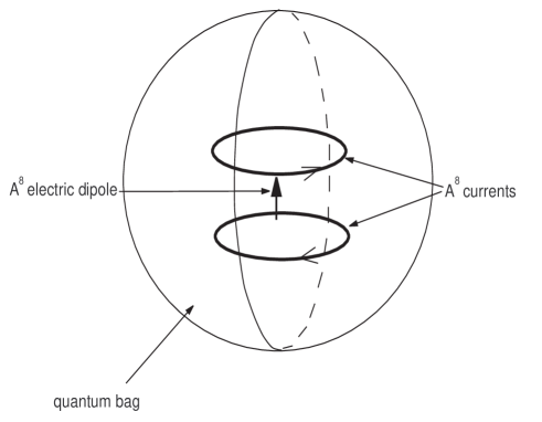
Figure 5: The schematical picture of the bag with confined color electromagnetic field as the model of glueball with spin $\hbar$.

Let us note that similar idea was presented in Ref. [16]. In this notice the author shows that the electromagnetic field angular momentum of a magnetic dipole and an electric charge may provide a portion of the nucleon’s internal angular momentum which is not accounted for by the valence quarks. From a rough estimate it is found that this electromagnetic field angular momentum could contribute to the nucleon’s spin $\approx 15\%\hbar$.

6 Discussion and conclusions

Now we would like to briefly list the results obtained above. First, we propose a model according to which one can approximately reduce quantum SU(3) Yang-Mills gauge theory to U(1) gauge theory with broken gauge symmetry and interacting with scalar fields. During such reduction the initial degrees of freedom $A^{B}_{\mu}$ are decomposed to $A^{a}_{\mu},A^{m}_{\mu}$ and $A^{8}_{\mu}$. $A^{a}_{\mu}$ and $A^{m}_{\mu}$ degrees of freedom are non-perturbatively quantized in such a way that they are similar to a non-linear oscillator, where $\left\langle A^{a,m}_{\mu}\right\rangle=0$ but $\left\langle\left(A^{a,m}_{\mu}\right)^{2}\right\rangle\neq 0$. $A^{8}_{\mu}$ degree of freedom remains almost classical and describe U(1) gauge theory with broken gauge symmetry. The quantized fields $A^{a}_{\mu},A^{m}_{\mu}$ approximately can be described as scalar fields $\phi^{m}$ and $\phi^{a}$ correspondingly. The obtained system of field equations has a self-consistent regular solution. Physically this solution presents a pure quantum bag which is described by interacting fields $\phi^{m}$ and $\phi^{a}$ and electromagnetic field $A^{8}_{\mu}$ which is confined inside the bag. The color electromagnetic field $A^{8}_{\mu}$ is the source of an angular momentum. The obtained object is a cloud of quantized fields with a spin (for some values of $\lambda_{1,2},k_{2}$ the spin can be equal to $\hbar$). We suppose that such an object can be considered as a model of glueball with spin one. The presence of the color electromagnetic field $A^{8}_{\mu}$ leads to an asymmetrical structure in the glueball and nucleon that probably can be proved experimentally.

Summarizing the results of this paper and Refs. [1], [17] one can say that the interaction between $A^{a}_{\mu}$ and $A^{m}_{\mu}$ degrees of freedom gives a quantum bag. If $A^{a}_{\mu}$ is non-quantized, in the result we have a flux tube with a longitudinal color electric field. If these degrees of freedom are quantized we have a quantum bag which can be considered as a model of glueball with spin zero. This paper and Ref. [18] show correspondingly that this bag can sustain an electromagnetic field and colorless spinor field (one can say that the bag is strong enough).

In this paper, we have shown that the interaction between the condensates $\left\langle A^{a}_{\mu}A^{a\mu}\right\rangle$, $\left\langle A^{m}_{\mu}A^{m\mu}\right\rangle$ and $\left\langle b_{\mu}b^{\mu}\right\rangle$ is a necessary condition for the existence of the quantum bag where the field $A^{8}$ is confined. One important thing here is that these calculations are non-perturbative and do not use Feynman diagram.

References

- [1] V. Dzhunushaliev, “Scalar model of the glueball”, to appear in Hadronic J., hep-ph/0312289.
- [2] Y. A. Simonov, “Analytic calculation of field-strength correlators”, hep-ph/0501182.
- [3] B. M. Gripaios, Phys. Lett. B 558, 250 (2003).
- [4] K.-I. Kondo, Phys. Lett. B 572, 210 (2003).
- [5] A. A. Slavnov, hep-th/0407194.
- [6] L. Stodolsky, Pierre van Baal and V. I. Zakharov, Phys. Lett. B 552, 214(2002).
- [7] F. V. Gubarev, L. Stodolsky, and V. I. Zakharov, Phys. Rev. Lett. 86, 2220 (2001).
- [8] F. V. Gubarev, V. I. Zakharov, Phys. Lett. B 501, 28 (2001).
- [9] J. A. Gracey, Phys. Lett. B 552, 101 (2003).
- [10] H. Verschelde, K. Knecht, K. Van Acoleyen and V. Vanderkelen, Phys. Lett. B 516, 307 (2001).
- [11] D. Dudal, H. Verschelde, J. A. Gracey, V. E. R. Lemes, M. S. Sarandy, R. F. Sobreiro and S. P. Sorella, JHEP 0401, 044 (2004); hep-th/0311194 v3.
- [12] W. Heisenberg, Introduction to the unified field theory of elementary particles., Max - Planck - Institut für Physik und Astrophysik, Interscience Publishers London, New York, Sydney, 1966; W. Heisenberg, Nachr. Akad. Wiss. Göttingen, N8, 111 (1953); W. Heisenberg, Zs. Naturforsch., 9a, 292 (1954); W. Heisenberg, F. Kortel und H. Mütter, Zs. Naturforsch., 10a, 425 (1955); W. Heisenberg, Zs. für Phys., 144, 1 (1956); P. Askali and W. Heisenberg, Zs. Naturforsch., 12a, 177 (1957); W. Heisenberg, Nucl. Phys., 4, 532 (1957); W. Heisenberg, Rev. Mod. Phys., 29, 269 (1957).
- [13] A. Di Giacomo, H.G. Dosch, V.I. Shevchenko and Yu. A. Simonov, Phys. Rep., 372, 319 (2002), hep-ph/0007223.
- [14] Yu. A. Simonov, “Selfcoupled equations for the field correlators”, hep-ph/9712250.
- [15] X. d. Li and C. M. Shakin, Phys. Rev. D 70 (2004) 114011.
- [16] D. Singleton, Phys. Lett. B427, 155 (1998).
- [17] V. Dzhunushaliev, “The colored flux tube” to appear in Hadronic J., hep-ph/0307274.
- [18] V. Dzhunushaliev, “Glueball filled with quark field as a model of nucleon” to appear in Hadronic J., hep-ph/0408236.