Some Recent Advances in Bound–State Quantum Electrodynamics

Abstract

We discuss recent progress in various problems related to bound-state quantum electrodynamics: the bound-electron $g$ factor, two-loop self-energy corrections and the laser-dressed Lamb shift. The progress relies on various advances in the bound-state formalism, including ideas inspired by effective field theories such as Nonrelativistic Quantum Electrodynamics. Radiative corrections in dynamical processes represent a promising field for further investigations.

1 Introduction

This is a brief summary of a number of recent advances in our understanding of bound-state quantum electrodynamic (QED) effects. The topics are (i) two-loop corrections to the bound-electron $g$ factor, (ii) higher-order two-loop corrections to the self-energy of a bound electron, and (iii) the laser-dressed Lamb shift.

The first two of these rather diverse topics are related to two-loop effects. The investigation of these is simplified considerably by the use of effective field-theory techniques inspired by Nonrelativistic QED (NRQED) [1, 2, 3]. The Wilson coefficients multiplying the effective operators in the NRQED Lagrangian are matched against those of the full relativistic theory, providing a simplified framework for the calculation of bound-state effects. Scale-separation parameters such as the photon mass $\mu$ are cancelled at the end of the calculation. The analysis of higher-order corrections to the $g$ factor of the bound electron is simplified further by a transformation to the length gauge, which results in a lesser number of terms to be considered than would be necessary in the velocity gauge. This fact has inspired the development of Long-wavelength QED (LWQED) [4], a theory which is obtained after Power–Zienau and Foldy–Wouthuysen transformations of the first-quantized Lagrangian; the second quantization is carried out by formulating the path integral. Consequently, an improved understanding and a tremendous simplification results for the calculation of a number of QED corrections for bound states, such as the $g$ factor and higher-order corrections to the self-energy.

A further field of recent studies has been concerned with the interaction of a laser-dressed bound electron with the radiation field [5, 6, 7, 8]. This process entails corrections which can only be understood if the analysis is carried out right from the start in the framework of the laser-dressed states, which are the eigenstates of the quantized atom-laser Hamiltonian in the rotating-wave approximation [9].

2 Bound-electron $g$ factor

In this section, we briefly summarize the results of a recent investigation [10] of the bound-electron $g$ factor, which is based on NRQED. The central result of this investigation is the following semianalytic expansion in powers of $Z\alpha$ and $\ln(Z\alpha)$ for the bound-electron $g$ factor ($n{\rm S}$ state) in the non-recoil limit, which is the limit of an infinite nuclear mass:

$$g(n{\rm S}) =\underbrace{2-\frac{2\,(Z\alpha)^{2}}{3\,n^{2}}+\frac{(Z\alpha)^{4}}{n^{3}}\,\left(\frac{1}{2n}-\frac{2}{3}\right)+{\cal O}{(Z\alpha)^{6}}}_{\mbox{Breit (1928), Dirac theory}}$$

$$+\underbrace{{\frac{\alpha}{\pi}}\,\left\{{2\times\frac{1}{2}}\,{\bigg{(}}1+\frac{(Z\alpha)^{2}}{6n^{2}}{\bigg{)}}+\frac{(Z\alpha)^{4}}{n^{3}}{\bigg{\{}}a_{41}\,{\ln}[(Z\alpha)^{-2}]+a_{40}{\bigg{\}}}+{\cal O}(Z\alpha)^{5}\right\}}_{\mbox{one-loop correction}}$$

$$+\underbrace{{\left(\frac{\alpha}{\pi}\right)^{2}}\,\left\{{-0.656958}\,{\bigg{(}}1+\frac{(Z\alpha)^{2}}{6n^{2}}{\bigg{)}}+\frac{(Z\alpha)^{4}}{n^{3}}{\bigg{\{}}b_{41}\,{\ln}[(Z\alpha)^{-2}]+b_{40}{\bigg{\}}}+{\cal O}(Z\alpha)^{5}\right\}}_{\mbox{two-loop correction}}$$

$$+{\cal O}(\alpha^{3})\,.$$ (1)

This expansion is valid through the order of two loops (terms of order $\alpha^{3}$ are neglected). The notation is in part inspired by the usual conventions for Lamb-shift coefficients: the (lower case) $a$ terms denote the one-loop effects, with $a_{kj}$ denoting the coefficient of a term proportional to $\alpha\,(Z\alpha)^{k}\,{\ln}^{j}[(Z\alpha)^{-2}]$. The $b$ terms denote the two-loop corrections, with $b_{kj}$ multiplying a term proportional to $\alpha^{2}\,(Z\alpha)^{k}\,{\ln}^{j}[(Z\alpha)^{-2}]$. In [10], complete results are derived for the coefficients $a_{41}$, $a_{40}$ and $b_{41}$.

In general, the expression corresponding to (2) for a free electron is obtained by letting the parameter $Z\alpha\to 0$ in every term of the loop expansion (expansion in powers of $\alpha$). In this limit, the known free-electron two-loop result is recovered [11, 12, 13, 14, 15, 16, 17].

Figure 1: Feynman diagrams for the two-loop self-energy corrections to the bound-electron $g$-factor.

Up to the relative order $(Z\alpha)^{2}$, the free-electron contribution in one-, two-, and higher-loop order is multiplied by a relative factor

$$1+(Z\alpha)^{2}\,a_{20}=1+(Z\alpha)^{2}\,b_{20}=1+\frac{(Z\alpha)^{2}}{6n^{2}}\,.$$ (2)

This result consequently holds for the three-loop and the four-loop term not shown in Eq. (2). The applicability of the relative factor (2) to the two-loop term, valid through $(Z\alpha)^{2}$, had been stressed previously in [18]. The result in Eq. (2) had been obtained originally in [19, 20, 21, 22, 23] (for the 1S state). As is evident from Eq. (2), the correction of relative order $(Z\alpha)^{2}$ is different on the level of the tree-level diagrams and reads $g(n{\rm S})\sim 2\times[1-(Z\alpha)^{2}/(3n^{2})]$.

Explicit results for the coefficients in (2), restricted to the one-loop self-energy, read [10]

$$a_{41}(n{\rm S}) =\frac{32}{9}\,,$$ (3a)

$$a_{40}(n{\rm S}) =\frac{73}{54}-\frac{5}{24n}-\frac{8}{9}\,\ln k_{0}(n{\rm S})-\frac{8}{3}\,\ln k_{3}(n{\rm S})\,.$$ (3b)

Here, $\ln k_{0}(nS)$ is the Bethe logarithm for an $nS$ state, and $\ln k_{3}(nS)$ is a generalization of the Bethe logarithm to a perturbative potential of the form $1/r^{3}$. Vacuum polarization adds a further $n$-independent contribution of $(-16/15)$ to $a_{40}$ [24]. The Bethe logarithms for 1S and 2S [25] read

$$\ln k_{0}(1{S}) = 2.984~{}128~{}555\,,$$ (4a)

$$\ln k_{0}(2{S}) = 2.811~{}769~{}893\,,$$ (4b)

and the corresponding values for $\ln k_{3}$ read [10]

$$\ln k_{3}(1{S}) = 3.272~{}806~{}545\,,$$ (5a)

$$\ln k_{3}(2{S}) = 3.546~{}018~{}666\,.$$ (5b)

The quantity $\ln k_{3}(n{\rm S})$ is defined as,

$$\int_{0}^{\epsilon}{\rm d}k\,k^{2}\,\langle\phi|\mbox{\boldmath$r$}\,\frac{1}{E-H_{S}-k}\,\frac{1}{r^{3}}\,\frac{1}{E-H_{S}-k}\,\mbox{\boldmath$r$}\,|\phi\rangle=-4\,\frac{(Z\alpha)^{3}}{n^{3}}\,\left[\ln\frac{\mu}{(Z\alpha)^{2}}+\frac{5}{6}-\ln k_{3}\right]$$ (6)

where the ultraviolet cutoff $\epsilon$ is to be understood in the sense of [2], and the matching of the noncovariant cutoff $\epsilon$ to the covariant photon mass $\mu$ is given as (see [26], pp. 361–362)

$$\ln\left(\frac{2\epsilon}{m}\right)\to\ln\left(\frac{\mu}{m}\right)+\frac{5}{6}\,.$$ (7)

However, this replacement is not unique and the constant term depends on the actual form of the integrand. A different replacement has to be used for some of the low-energy photon corrections to the $g$ factor [10].

The results for the two-loop coefficients read

$$b_{41}(n{\rm S}) =\frac{56}{9}\,,$$ (8a)

$$b_{40}(1{\rm S}) =-18.5(5.5)\,.$$ (8b)

Here, the result for $b_{40}$ is an estimate based on an explicit calculation of a large contribution due to low-energy virtual photons, and an estimate of the remaining, unknown contribution due to high-energy virtual photons. The dominant logarithmic two-loop term $b_{41}$ is caused exclusively by the two-loop self-energy diagrams in Fig. 1 alone. The other two-loop diagrams, which include closed fermion loops, can be found in Fig. 21 of [27]. The logarithmic term $b_{41}$ is, however, exclusively related to the gauge-invariant subset displayed in Fig. 1.

The newly calculated $a_{41}$, $a_{40}$ and $b_{41}$ are bound-state corrections to the electron $g$-factor of order $(\alpha/\pi)\,(Z\alpha)^{4}$ and $(\alpha/\pi)^{2}\,(Z\alpha)^{4}$, multiplied by logarithmic terms. These corrections are (at $Z=1$) formally of order $\alpha^{5}$ and $\alpha^{6}$ and therefore of the same order of magnitude as the tenth- and twelfth-order corrections to the free-electron anomaly, which barely are of experimental or theoretical significance at the current level of accuracy. One may therefore ask why these binding corrections are of any phenomenological significance. The reason is that at somewhat higher $Z$, the situation changes drastically, due to $Z^{4}$ scaling of the binding corrections. In addition, due to numerically large coefficients and logarithmic factors, the ‘‘hierarchy’’ of the corrections changes drastically. Roughly, one may say that at $Z=1$, the bound-electron anomalous magnetic moment is approximately independent of binding corrections of order $(\alpha/\pi)\,(Z\alpha)^{4}$ and higher, whereas for higher $Z$, the situation is reversed, and the binding corrections to the one- and two-loop contributions are numerically much more significant than the higher-loop free-electron corrections. This ‘‘transition from free to bound-state quantum electrodynamics’’ as a function of $Z$ is a somewhat peculiar feature of the bound-electron $g$-factor.

For, example, we consider the ratio

$$r_{1}(Z)=\frac{\displaystyle\left(\frac{\alpha}{\pi}\right)\,(Z\alpha)^{4}\,\ln[(Z\alpha)^{-2}]}{\displaystyle\left(\alpha/\pi\right)^{4}}\,,$$ (9)

which gives an order-of-magnitude estimate for the the ratio of the one-loop self-energy binding correction to the eighth-order anomalous magnetic moment of the free electron. We have

$$r_{1}(Z=1)\approx 2\,,\qquad r_{1}(Z=10)\approx 10^{4}\gg 1\,.\qquad$$ (10)

For the two-loop logarithmic binding correction, we have

$$r_{2}(Z)=\frac{\displaystyle\left(\frac{\alpha}{\pi}\right)^{2}\,(Z\alpha)^{4}\,\ln[(Z\alpha)^{-2}]}{\displaystyle\left(\alpha/\pi\right)^{4}}$$ (11)

and consequently

$$r_{2}(Z=1)\approx 0.2<1\,,\qquad r_{2}(Z=10)\approx 2\times 10^{3}\gg 1\,.\qquad$$ (12)

As is evident from these considerations, the $(Z\alpha)^{4}$ one-loop and two-loop binding corrections are roughly of the same order of magnitude as the highly problematic four-loop corrections [28, 29, 30] for the free electron. However, the situation changes drastically even at very moderate nuclear charge numbers, and the binding corrections to the one-loop and two-loop contributions become dominant over the higher-loop effects.

The NRQED one-loop calculation [10] is divided into three parts, the first of which entails fully relativistic form-factor corrections including lower-order terms, the second of which corresponds to a spin-dependent scattering amplitude, and the third of which is a low-energy Bethe-logarithm type correction that contains $\ln k_{0}$ and $\ln k_{3}$. The one-loop correction in Eq. (2) can therefore be written in a natural way as $\delta g^{(1)}=g_{1}^{(1)}+g_{2}^{(1)}+g_{3}^{(1)}$, where

$$g_{1}^{(1)} =\frac{\alpha}{\pi}\biggl{[}1+\frac{(Z\alpha)^{2}}{6\,n^{2}}-\frac{(Z\alpha)^{4}}{n^{3}}\,\left(\frac{7}{6}+\frac{5}{24n}+\frac{16}{3}\,\ln\mu\right)\biggr{]}\,,$$ (13a)

$$g_{2}^{(1)} =\frac{\alpha}{\pi}\,\frac{(Z\alpha)^{4}}{n^{3}}\,\Bigl{(}4+\frac{16}{9}\,\ln\mu\Bigr{)}\,,$$ (13b)

$$g_{3}^{(1)} =\frac{\alpha}{\pi}\,\frac{(Z\alpha)^{4}}{n^{3}}\,\frac{32}{9}\,\biggl{[}\ln\frac{\mu}{(Z\alpha)^{2}}-\frac{5}{12}-\frac{\ln k_{0}}{4}-\frac{3}{4}\,\ln k_{3}\biggr{]}\,.$$ (13c)

The new contribution of order $(Z\alpha)^{4}$ can be compared with the numerical results for the self-energy correction [31, 32] complete to all orders in $Z\alpha$. Assuming correctness of the logarithmic term in Eq. (13), a fit to numerical data yields $a_{40}^{(1)}({\rm 1S})=-10.2(1)$ and $a_{40}^{(1)}({\rm 2S})=-10.6(1.2)$ for the constant term, in excellent agreement with the analytic results which read $a_{40}^{(1)}({\rm 1S})=-10.236~{}524~{}318(1)$ and $a_{40}^{(1)}({\rm 2S})=-10.707~{}715~{}607(1)$ .

Having verified the consistency of the analytic [10] and numerical results [31, 32], an interpolation procedure [33] may now be used to extract a more accurate theoretical prediction at low and intermediate nuclear charge numbers, if combined with numerical results at higher $Z$ [31]. Thus, the results in Eqs. (3) and (8) may be used in order to infer improved theoretical predictions for the bound-electron $g$ factor, notably in the experimentally important special cases of hydrogenlike carbon [34] and oxygen [35]. Alternatively, the improved status of the theory may be used in order to infer a more accurate value of the electron mass. Specifically, the value from the carbon measurement [34], using the new theory, reads

$$m(^{12}{\rm C}^{5+})=0.000\,548\,579\,909\,41\,(29)(3)\ {\rm u}\,.$$ (14)

The first error comes from the experiment [34], and the second error corresponds to the theoretical uncertainty. The conclusion is that a further improvement of the experiment could lead to a much better determination of the electron mass; the new theory provides room for at least an improved determination by one order of magnitude.

For the calculation of yet higher-order binding corrections to the one-loop and two-loop contributions, a detailed understanding of the two-loop form-factors, including their slopes, is required. The most recent calculations of these effects, in both dimensional and photon-mass regularizations, can be found in [36, 37, 38].

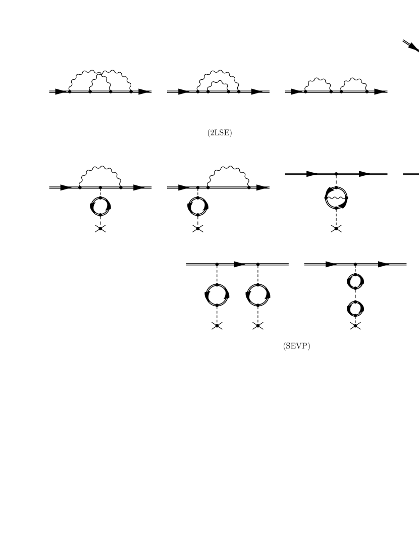
Figure 2: The two-loop corrections to the Lamb shift in hydrogenlike systems fall naturally into three gauge-invariant subsets, which are the pure two-loop self-energy terms (2LSE), the vacuum-polarization correction to the virtual-photon line in the self-energy (SVPE), and the self-energy vacuum-polarization and pure two-loop vacuum-polarization corrections (SEVP). The two-loop Bethe logarithm is a numerically large correction to the nonlogarithmic term of order $\alpha^{2}(Z\alpha)^{6}$ and it is exclusively related to the 2LSE subset; however, for a complete result in this order, contributions from the other gauge-invariant subsets will have to be considered as well.

3 Two-loop Bethe logarithms

As is well known [39, 40, 41, 42, 43, 44, 45, 46], the two-loop Lamb shift $\Delta E^{(2)}$, in the limit of an infinite nuclear mass, may be written as

$$\Delta E^{(2)}=\left(\frac{\alpha}{\pi}\right)^{2}\,\frac{(Z\alpha)^{4}\,m_{\rm e}\,c^{2}}{n^{3}}\,H(Z\alpha)\,.$$ (15)

For S states, the dimensionless function $H(Z\alpha)$, has a semianalytic expansion of the form

$$H(Z\alpha)= B_{40}+(Z\alpha)\,B_{50}$$

$$+(Z\alpha)^{2}\,\left[B_{63}\,\ln^{3}[(Z\alpha)^{-2}]+B_{62}\,\ln^{2}[(Z\alpha)^{-2}]+B_{61}\,\ln[(Z\alpha)^{-2}]+B_{60}\right]\,,$$ (16)

where we ignore higher-order terms, and upper case is used for the $B_{ij}$ coefficients that multiply terms of order $\alpha^{2}\,(Z\alpha)^{i}\,\ln^{j}[(Z\alpha)^{-2}]\,m_{\rm e}\,c^{2}$. The coefficients, restricted to the two-photon self-energy diagrams (Fig. 2), read as follows

$$B^{\rm(2LSE)}_{63}(n{\rm S}) = -\frac{8}{27}=-0.296296\,,$$ (17a)

$$B^{\rm(2LSE)}_{62}(1{\rm S}) = \frac{16}{27}-\frac{16}{9}\,\ln(2)=-0.639\,669\,,$$ (17b)

$$B^{\rm(2LSE)}_{62}(n{\rm S}) = B^{\rm(2LSE)}_{62}(1{\rm S})+\frac{16}{9}\left(\frac{3}{4}+\frac{1}{4n^{2}}-\frac{1}{n}-\ln(n)\!+\!\Psi(n)+C\right)\,.$$ (17c)

The $n$-dependence of $B_{61}$ has been clarified in [46, 47]

$$B^{\rm(2LSE)}_{61}(n{\rm S}) = B^{\rm(2LSE)}_{61}(1{\rm S})+\frac{4}{3}\,\left[N(n{\rm S})-N(1{\rm S})\right]$$ (18)

$$+\!\left(\frac{80}{27}-\frac{32}{9}\,\ln(2)\right)\left(\frac{3}{4}+\frac{1}{4n^{2}}-\frac{1}{n}-\ln(n)\!+\!\Psi(n)\!+\!C\right)\,,$$

where $C=0.577216\dots$ is Euler’s constant, $\Psi(n)$ is the logarithmic derivative of the Gamma function, and $N(n{\rm S})$ is related to a correction to the Bethe logarithm induced by a Dirac-delta potential. Explicit values for $N(n{\rm S})$ can be found in [47] ($n=1,\dots,8$).

Figure 3: The integration regions for the two virtual photons in the two-loop self-energy problem comprise a low-energy regime with two low-energy photons, which gives rise to $b_{L}$. The middle-energy regions with one low-energy and a one high-energy photon give rise to $b_{M}$. The high-energy contribution $b_{F}+b_{H}$ is as yet unknown.

The $B_{60}$ coefficients are the sum of several contributions

$$B^{\rm(2LSE)}_{60}(n{\rm S}) = b_{L}+b_{M}+\left\{b_{F}+b_{H}+b_{\rm VP}\right\}\,,$$ (19a)

$$b_{L} = b_{L}(n{\rm S})\;\sim\;\mbox{two-loop Bethe logarithm, two soft photons}\,,$$ (19b)

$$b_{M} = b_{M}(n{\rm S})\;=\;\frac{10}{9}\,N(n{\rm S})\;\sim\;\mbox{one soft, one hard photon}\,,$$ (19c)

$$b_{F} \sim \mbox{soft electron momenta, two hard photons}\,,$$ (19d)

$$b_{H} \sim \mbox{hard electron momenta, two hard photons}\,,$$ (19e)

$$b_{\rm VP} \sim \mbox{vacuum-polarization corrections}\,.$$ (19f)

Only the terms $b_{L}+b_{M}$ are currently known [48, 49] (see also Fig. 2). The contributions in curly brackets in Eq. (19a) remain to be evaluated. However, an estimate for the total value of $B_{60}$ may be obtained,

$$B_{60}(n{\rm S}) = b_{L}+b_{M}+\left\{b_{F}+b_{H}+b_{\rm VP}\right\}\,,$$

$$B_{60}(n{\rm S}) \approx b_{L}+b_{M}\;\pm\;15\,\%\,.$$ (20)

This estimate [48, 49] is based on corresponding one-loop calculations, where the low-energy virtual photons give the by far dominant contribution to the constant term [2]. The results for the two-loop Bethe logarithms of S states read [48, 49]

$$b_{L}(1S) = -81.4(3)\,,$$ (21a)

$$b_{L}(2S) = -66.6(3)\,,$$ (21b)

$$b_{L}(3S) = -63.5(6)\,,$$ (21c)

$$b_{L}(4S) = -61.8(8)\,,$$ (21d)

$$b_{L}(5S) = -60.6(8)\,,$$ (21e)

$$b_{L}(6S) = -59.8(8)\,.$$ (21f)

A few clarifying remark might be in order. The $B_{60}$ coefficient multiplies a correction of order $\alpha^{2}(Z\alpha)^{6}$, which is effectively an order-$\alpha^{8}$ contribution to the energy levels of hydrogen ($Z=1$). In order to complete the calculation at this order of magnitude, it would also be necessary to consider the four-loop Dirac form-factor slope of the electron, as well as the three-loop binding correction of order $\alpha^{3}\,(Z\alpha)^{5}\,m_{\rm e}\,c^{2}$ [50]. The three-loop slope has recently been evaluated in [51], completing the theory of energy levels in hydrogen up to the order of $\alpha^{7}$.

4 Laser-dressed Lamb shift

In the recent past, seminal advances have been obtained both in the techniques of high-precision spectroscopy (e.g., [52]), and in the coherent preparation and manipulation of media by external electromagnetic fields [53, 54]. Thus it is desirable to study the bound electrons interacting simultaneously both with the quantized radiation field and with an external driving field. An accurate theory of such systems, including all dynamic effects, might eventually open a possibility for a whole new class of high-precision experiments, provided that technical problems related to the required highly accurate intensity stabilization of the laser (and others) can be solved. Traditionally, radiative and relativistic corrections are treated with methods of QED, whereas studies related to the dynamical nature of the interaction of matter with driving laser fields are the domain of Quantum Optics (QO). Obviously, a treatment of bound electrons in the presence of both the radiation field and external driving fields requires a combination of ideas from both subject areas: While, a priori, the essential-state approximation of QO [53] is not sufficient to obtain the accuracy of QED, a perturbative treatment of the interaction of the bound electron with a strong external (laser) field as in QED is hopeless because of the large coupling parameter.

In [5, 6, 7], an atom with two relevant energy levels driven by a strong near-resonant monochromatic laser field is studied as the easiest model system for the above problem. The incoherent part of the resonance fluorescence spectrum emitted by this system in QO is known as the Mollow spectrum, where the coupling strength is characterized by the the Rabi frequency $\Omega$ defined as ($\hbar=\epsilon_{0}=c=1$)

$$\Omega=-q\left<e|{\mbox{\boldmath$x$}}\cdot{\mbox{\boldmath$\epsilon$}}_{\rm L}|g\right>{\cal E}_{\rm L}\,,$$ (22)

for a driving laser field ${\mbox{\boldmath$E$}}_{\rm L}(t)={\cal E}_{\rm L}{\mbox{\boldmath$\epsilon$}}_{\rm L}\cos(\omega_{\rm L}t)$ with frequency $\omega_{\rm L}$, macroscopic classical amplitude ${\cal E}_{\rm L}$ and polarization ${\mbox{\boldmath$\epsilon$}}_{\rm L}$. Here, $q=-|q|$ is the elementary charge. The corresponding coupling constant $g_{\rm L}$ for the interaction of a quantized driving laser field with the main atomic transition is defined by

$$g_{\rm L}=-q\,\langle g|\mbox{\boldmath$\epsilon$}_{\rm L}\cdot\mbox{\boldmath$x$}|e\rangle\,{\cal E}_{\rm L}^{\rm(\gamma)}\,,$$ (23)

where ${\cal E}_{\rm L}^{\rm(\gamma)}=\sqrt{\omega_{\rm L}/2V}$ is the electric laser field per photon and $V$ is the quantization volume. The matching of the electric field per photon with the corresponding classical macroscopic electric field ${\cal E}_{\rm L}$ is then given by

$$2\>\sqrt{n+1}\>{\cal E}_{\rm L}^{\rm(\gamma)}\>\longleftrightarrow\>{\cal E}_{\rm L}\,.$$ (24)

If $\Omega$ is larger than the natural decay width $\Gamma$ of the transition, then the Mollow spectrum approximately consists of one central and two sideband peaks of Lorentzian shape, which are located symmetrically around the driving laser field frequency. The sideband peaks are shifted from the driving field frequency by the generalized Rabi frequency $\Omega_{\textrm{R}}=\sqrt{\Omega^{2}+\Delta^{2}}$, where $\Delta=\omega_{\textrm{L}}-\omega_{\textrm{R}}$ is the detuning of the laser field frequency $\omega_{\textrm{L}}$ with regard to the atomic transition frequency $\omega_{\textrm{R}}$. The shape of the Mollow spectrum may easily be explained in terms of the dressed states, which are defined as the eigenstates of the quantum optical interaction picture Hamiltonian describing the matter-light interaction. In transferring to the dressed state picture, the interaction with the driving laser field is accounted for to all orders.

Thus, when evaluating radiative and relativistic corrections to the Mollow spectrum, it is natural to start the analysis from the dressed-state basis as opposed to the unperturbed atomic bare-state basis. In [5, 6], it was shown that this distinction in fact has to be made. It is not sufficient to modify the energies (which enter in the formula for the dressed states) according to the usual bare-state Lamb shift in order to obtain the correct result for the corrections to the Mollow spectrum. Instead, at nonvanishing detuning and nonvanishing Rabi frequency, a treatment starting from the dressed-state basis leads to an additional nontrivial correction term. This term gives rise to a shift of the Mollow sidebands relative to the central peak given by

$$\delta\omega_{\pm}^{(C)}=\mp{\cal C}\,\frac{\Omega^{2}}{\sqrt{\Omega^{2}+\Delta^{2}}}\,,$$ (25)

where

$${\cal C} = \frac{\alpha}{\pi}\,\ln[(Z\alpha)^{-2}]\,\frac{\left<\mbox{\boldmath$p$}^{2}\right>_{g}+\left<\mbox{\boldmath$p$}^{2}\right>_{e}}{m^{2}}$$ (26)

is a dimensionless constant. Here, the notation $\langle.\rangle_{g}$ and $\langle.\rangle_{e}$ denotes the expectation value evaluated with the ground or excited atomic state, respectively.

Inspired by the interpretation of the bare Lamb shift correction in terms of a ‘‘summed’’ shift as in [5, 6], this additional correction can be interpreted as a modification to the Rabi frequency:

$$\delta\overline{\omega}^{(C)}_{\pm}=\pm\left(\sqrt{\Omega^{2}\,(1-{\cal C})^{2}+\Delta^{2}}-\sqrt{\Omega^{2}+\Delta^{2}}\right)\,,$$ (27)

with $\delta\overline{\omega}^{(C)}_{\pm}\approx\delta\omega_{\pm}^{(C)}$ because of the smallness of the correction. It should be noted that this interpretation in terms of a summation is not trivial and was shown to be valid up to first order in the correction.

In [5, 7], the leading relativistic and radiative corrections up to relative orders $(Z\alpha)^{2}$ and $\alpha(Z\alpha)^{2}$, respectively, have been evaluated, as well as all other relevant correction terms up to the specified order of approximation. It turns out that all corrections may be interpreted as either corrections to the Rabi frequency $\Omega$ or as corrections to the detuning $\Delta$, such that one can define the fully corrected generalized Rabi frequency $\Omega^{(j)}_{\mathcal{C}}$ by

$$\Omega^{(j)}_{\mathcal{C}}=\sqrt{\Omega^{2}\cdot\left(1+{\hat{\Omega}_{\rm rad}^{(j)}}\right)^{2}+\left(\Delta-{\Delta^{(j)}_{\rm rad}}\right)^{2}}\,.$$ (28)

Here, $\hat{\Omega}_{\rm rad}^{(j)}$ contains all corrections to the Rabi frequency, namely the relativistic and radiative corrections to the transition dipole moment, field-configuration dependent corrections, higher-order corrections to the self-energy, and corrections to the secular approximation. $\Delta^{(j)}_{\rm rad}$ consists of all corrections to the detuning, i.e. the bare Lamb shift, Bloch-Siegert shifts, and off-resonant radiative corrections. The superscript $(j)$ indicates the dependence of the result on the total angular momentum quantum number.

Equation (28) summarizes the main result of this study: In the presence of driving laser fields, the usual bare state Lamb shift of the atomic states is augmented by additional correction terms. These in part depend on the laser field parameters $\Omega$ and $\Delta$, which span a two-dimensional parameter manifold determining the actual value of the dynamical Lamb shift.

A promising candidate for the experiment are the hydrogen $1S_{\nicefrac{{1}}{{2}}}\leftrightarrow 2P_{\nicefrac{{1}}{{2}}}$ and $1S_{\nicefrac{{1}}{{2}}}\leftrightarrow 2P_{\nicefrac{{3}}{{2}}}$ transitions. We consider here as a specific example the $1S_{\nicefrac{{1}}{{2}}}\leftrightarrow 2P_{\nicefrac{{1}}{{2}}}$ transition with $\Omega=1000\cdot\Gamma_{\nicefrac{{1}}{{2}}}$ and $\Delta=50\cdot\Gamma_{\nicefrac{{1}}{{2}}}$ as the laser field parameters. The Rabi frequency is shifted with respect to the leading-order expression $\Omega_{\rm R}=\sqrt{\Omega^{2}+\Delta^{2}}$ by relativistic and radiative corrections as follows,

$$\pm\left(\Omega^{(\nicefrac{{1}}{{2}})}_{\mathcal{C}}-\Omega_{\rm R}\right)=\pm 738.282(60)\cdot 10^{6}\>\rm{Hz}\,.$$ (29)

This driving laser field parameter set is expected to be within reach of improvements of the currently available Lyman-$\alpha$ laser sources [55] in the next few years. The corresponding result for the $1S_{\nicefrac{{1}}{{2}}}\leftrightarrow 2P_{\nicefrac{{3}}{{2}}}$ transition with $\Omega=1000\cdot\Gamma_{\nicefrac{{3}}{{2}}}$, $\Delta=50\cdot\Gamma_{\nicefrac{{3}}{{2}}}$ is

$$\pm\left(\Omega^{(\nicefrac{{3}}{{2}})}_{\mathcal{C}}-\Omega_{\rm R}\right)=\pm 734.871(60)\cdot 10^{6}\>\rm{Hz}\,.$$ (30)

All given uncertainties are due to unknown higher-order terms [7].

By a comparison to experimental data, one may verify the presence of dynamical leading-logarithmic correction to the dressed-state radiative shift in Eq. (25), which cannot be explained in terms of the bare Lamb shift alone. This allows to address questions related to the physical reality of the dressed states. On the other hand, the comparison with experimental results could also be used to interpret the nature of the evaluated radiative corrections in the sense of the summation formulas which lead to the interpretation of the shifts as arising from relativistic and radiative corrections to the detuning and the Rabi frequency.

5 Conclusions

One of the obvious conclusions to be drawn from the recent advances in bound-state quantum electrodynamics is as follows. A widespread opinion has been invalidated which suggested that two-loop corrections to the bound-electron $g$ factor, and two-loop corrections to the Lamb shift in higher order might be a severe, if not insurmountable, obstacle against further theoretical progress. Quite to the contrary, the recent advances have shown that an understanding of these effects is feasible to a good accuracy. While some important contributions remain to be evaluated, the further program (e.g., the evaluation of the remaining high-energy parts) is clearly defined, and decisive first steps toward a much improved understanding have been accomplished.

Further advances are possible both on the experimental as well as on the theoretical side: concerning the $g$ factor, the recent theoretical progress allows for an order-of-magnitude improvement of the value for the electron mass based on a potential new measurement alone. Regarding the Lamb shift in hydrogen and low-$Z$ hydrogenlike systems, one has recently gained an improved understanding of the binding corrections of order $\alpha^{2}\,(Z\alpha)^{6}\,\ln^{j}[(Z\alpha)^{-2}]\,m_{\rm e}\,c^{2}$ (where $j$ may assume the values $j=0,\dots,3$). Recent numerical investigations in the regime of intermediate nuclear charge numbers [56] have also contributed toward an improvement of our understanding. The extrapolation of the low-$Z$ results by deferred Padé approximants [57] suggests a rather good general consistency of both approaches, while some issues regarding the consistency of the analytic and numerical approaches remain to be addressed [56].

Other progress concerns the modifications of radiative corrections in dynamical processed as opposed to $S$-matrix energy shifts. The laser-dressed Lamb shift [5, 6, 7, 8] is a dynamical correction to the dressed-state [9] quasi-energies. The self-energy, in this case, gives the by far dominant effect. While the bulk of the laser-dressed Lamb shift can be understood in terms of a radiative correction to the detuning, which is taken into account in a natural way by evaluating the detuning in terms of the observed (low-intensity) resonance frequency of the transition, a few tiny shifts persist which can only be understood if the system is treated in the dressed-state picture right from the start. The dynamic Lamb shift is an effect which depends on two parameters that determine the dynamics of the system: (i) the detuning and (ii) the Rabi frequency. Therefore, the dynamical Lamb shift could be mapped out as a function of these parameters in a possible experiment. A rather promising candidate for a possible measurement would be based on the hydrogen 1S–2P${}_{\nicefrac{{1}}{{2}}}$ transition [5]. However, a very attractive alternative would be provided by a forbidden M1 transition [58] in Ar XIV, $2s^{2}\,2p\,{}^{2}{\rm P}_{\nicefrac{{1}}{{2}}}$–${}^{2}{\rm P}_{\nicefrac{{3}}{{2}}}$, provided the many-body QED effects can be treated to sufficient accuracy. The system in question is described very well by a two-level formalism, and the resonance line width is small.

References

- [1] W. E. Caswell and G. P. Lepage, Phys. Lett. B 167, 437 (1986).
- [2] K. Pachucki, Ann. Phys. (N.Y.) 226, 1 (1993).
- [3] A. Pineda and J. Soto, Phys. Rev. D 59, 016005 (1998).
- [4] K. Pachucki, Phys. Rev. A 69, 052502 (2004).
- [5] U. D. Jentschura, J. Evers, M. Haas, and C. H. Keitel, Phys. Rev. Lett. 91, 253601 (2003).
- [6] U. D. Jentschura and C. H. Keitel, Ann. Phys. (N.Y.) 310, 1 (2004).
- [7] J. Evers, U. D. Jentschura, and C. H. Keitel, Relativistic and Radiative Corrections to the Mollow Spectrum, e-print quant-ph/0403202, submitted to Phys. Rev. A.
- [8] U. D. Jentschura, J. Evers, and C. H. Keitel, Relativistic and Radiative Corrections to Multi-Level Mollow–Type Spectra, Laser Physics, at press (special issue on the occasion of the 70th birthday of Prof. Herbert Walther).
- [9] C. Cohen-Tannoudji, in Aux frontières de la spectroscopie laser/Frontiers in Laser Spectroscopy, edited by R. Balian, S. Haroche, and S. Liberman (North-Holland, Amsterdam, 1975), pp. 4–104.
- [10] K. Pachucki, U. D. Jentschura, and V. A. Yerokhin, Phys. Rev. Lett. 93, 150401 (2004).
- [11] R. Karplus and N. M. Kroll, Phys. Rev. 77, 536 (1950).
- [12] C. M. Sommerfield, Phys. Rev. 107, 328 (1957).
- [13] C. M. Sommerfield, Ann. Phys. (N.Y.) 5, 26 (1958).
- [14] A. Petermann, Helv. Phys. Acta 30, 407 (1957).
- [15] E. Remiddi, Nuovo Cim. A 11, 825 (1972).
- [16] E. Remiddi, Nuovo Cim. A 11, 865 (1972).
- [17] G. S. Adkins, Phys. Rev. D 39, 3798 (1989).
- [18] S. G. Karshenboim, in The Hydrogen Atom, edited by S. G. Karshenboim and F. S. Pavone (Springer, Berlin, 2001), pp. 651–663.
- [19] H. Grotch, Phys. Rev. Lett. 24, 39 (1970).
- [20] H. Grotch, Phys. Rev. A 2, 1605 (1970).
- [21] H. Grotch and R. A. Hegstrom, Phys. Rev. A 4, 59 (1971).
- [22] R. Faustov, Phys. Lett. B 33, 422 (1970).
- [23] R. Faustov, Nuovo Cim. 69, 37 (1970).
- [24] S. G. Karshenboim, Phys. Lett. A 266, 380 (2000).
- [25] G. W. F. Drake and R. A. Swainson, Phys. Rev. A 41, 1243 (1990).
- [26] C. Itzykson and J. B. Zuber, Quantum Field Theory (McGraw-Hill, New York, NY, 1980).
- [27] T. Beier, Phys. Rep. 339, 79 (2000).
- [28] T. Kinoshita and W. B. Lindquist, Phys. Rev. D 42, 636 (1990).
- [29] T. Kinoshita, IEEE Trans. Instrum. Meas. 44, 498 (1995).
- [30] V. W. Hughes and T. Kinoshita, Rev. Mod. Phys. 71, S133 (1999).
- [31] V. A. Yerokhin, P. Indelicato, and V. M. Shabaev, Phys. Rev. Lett. 89, 143001 (2002).
- [32] V. A. Yerokhin, P. Indelicato, and V. M. Shabaev, Phys. Rev. A 69, 052503 (2004).
- [33] V. G. Ivanov and S. G. Karshenboim, in The Hydrogen Atom, edited by S. G. Karshenboim and F. S. Pavone (Springer, Berlin, 2001), pp. 637–650.
- [34] H. Häffner, T. Beier, N. Hermanspahn, H.-J. Kluge, W. Quint, J. Verdú, and G. Werth, Phys. Rev. Lett. 85, 5308 (2000).
- [35] J. Verdú, S. Djekić, S. Stahl, T. Valenzuela, M. Vogel, G. Werth, T. Beier, H. J. Kluge, and W. Quint, Phys. Rev. Lett. 92, 093002 (2004).
- [36] R. Bonciani, P. Mastrolia, and E. Remiddi, Nucl. Phys. B 661, 289 (2003).
- [37] P. Mastrolia and E. Remiddi, Nucl. Phys. B 664, 341 (2003).
- [38] R. Bonciani, P. Mastrolia, and E. Remiddi, Nucl. Phys. B 676, 399 (2004).
- [39] T. Appelquist and S. J. Brodsky, Phys. Rev. A 2, 2293 (1970).
- [40] S. G. Karshenboim, JETP 76, 541 (1993), [ZhETF 103, 1105 (1993)].
- [41] K. Pachucki, Phys. Rev. Lett. 72, 3154 (1994).
- [42] M. I. Eides and V. A. Shelyuto, Phys. Rev. A 52, 954 (1995).
- [43] S. G. Karshenboim, J. Phys. B 29, L29 (1996).
- [44] S. G. Karshenboim, JETP 82, 403 (1996), [ZhETF 109, 752 (1996)].
- [45] S. G. Karshenboim, Z. Phys. D 39, 109 (1997).
- [46] K. Pachucki, Phys. Rev. A 63, 042503 (2001).
- [47] U. D. Jentschura, J. Phys. A 36, L229 (2003).
- [48] K. Pachucki and U. D. Jentschura, Phys. Rev. Lett. 91, 113005 (2003).
- [49] U. D. Jentschura, Two-Loop Bethe Logarithms for Higher Excited Levels, Phys. Rev. A (2004), at press.
- [50] M. I. Eides and V. A. Shelyuto, Phys. Rev. A 70, 022506 (2004).
- [51] K. Melnikov and T. v. Ritbergen, Phys. Rev. Lett. 84, 1673 (2000).
- [52] J. Reichert, M. Niering, R. Holzwarth, M. Weitz, T. Udem, and T. W. Hänsch, Phys. Rev. Lett. 84, 3232 (2000).
- [53] M. O. Scully and M. S. Zubairy, Quantum Optics (Cambridge University Press, Cambridge, 1997).
- [54] Z. Ficek and S. Swain, Quantum Interference and Coherence — Springer Series in Optical Sciences vol. 100 (Springer, Berlin, Heidelberg, New York, to appear in 2005, ISBN: 0-387-22965-5).
- [55] K. S. E. Eikema, J. Walz, and T. W. Hänsch, Phys. Rev. Lett. 86, 5679 (2001).
- [56] V. A. Yerokhin, P. Indelicato, and V. M. Shabaev, Two-loop self-energy correction to the ground-state Lamb shift in H-like ions, e-print hep-ph/0409048.
- [57] U. D. Jentschura, Phys. Lett. B 564, 225 (2003).
- [58] I. Draganić, J. R. Crespo López-Urrutia, R. DuBois, S. Fritzsche, V. M. Shabaev, R. S. Orts, I. I. Tupitsyn, Y. Zou, and J. Ullrich, Phys. Rev. Lett. 91, 183001 (2003).