Quasi-Particle Excitations
of the Higgs Vacuum at Finite Energy Density

Abstract

Real time excitations in the broken symmetry phase of the classical Abelian Higgs model are investigated numerically in the unitary gauge. Spectral equations of state of its constituent quasi-particles are extracted. Characteristic differences between the statistical correlations of the transverse and of the longitudinal vector modes with the Higgs field are exposed. A method is proposed for the reconstruction of the quasi-free composite field coordinates.

1 Introduction

The rearrangement of the multiplet structure of elementary fields in Gauge+Higgs models in the process of symmetry breaking is one of the most fundamental concepts upon which the Standard Model of elementary particle interactions is built [1, 2]. The transmutation of the pseudo-Goldstone field into the longitudinal polarisation state of massive vector bosons at the minimum of the effective potential has been successfully used in perturbative calculations. The absence of light (massless) fields from the spectra of the electroweak sector of the Standard Model was also tested non-perturbatively first at relatively strong coupling [3], later close to the continuum [4, 5]. Real time investigations of classical gauge field dynamics mostly concentrated on topological aspects of the process of baryogenesis, e.g. measuring Chern-Simons densities [6, 7], and on the emergence and the evolution of gauged strings [8, 9, 10].

The idea of far-from-equilibrium baryogenesis [11, 12, 13, 14, 15] led to increasingly detailed studies of the real time mechanism of the reheating of the Universe at the end of inflation. Features of the parametric resonance and tachyonic instability were first studied in simplified inflaton+Higgs systems [16, 17, 18, 19], realising the hybrid inflation scenario. In these systems the breaking of the global symmetry leads to the generation of Goldstone fields and related global topological excitations (e.g. strings). Recent numerical studies of Higgs systems started the detailed quantitative exploration of the real time excitation process of the Higgs and massive vector particles [20, 15, 10].

J. Smit et al. [20, 15] developed methods for the identification of the different physical degrees of freedom in the process of excitation in Coulomb and unitary gauges with help of measuring the corresponding dispersion relations. They measured the time variation of the corresponding number densities during tachyonic (spinodal) instability. In the unitary gauge they find significant differences between the early values taken by the number densities of the transversal and longitudinal degrees of freedom. The differences diminish when the system approaches equilibrium.

Our final goal in the real time investigation of the Abelian Gauge+Higgs system is to measure the evolution of the equations of state of its physical components during the reheating period. To achieve this we apply methods developed in our earlier investigation of pure scalar (inflaton+Higgs) systems [21, 19]. In order to understand the nature of the final state to which the system eventually relaxes in this paper a careful numerical study of the real time fluctuations in equilibrium systems with low energy densities is presented. We extract the equilibrium equations of state of the different quasi-particle species and an attempt will be described to establish the corresponding effective field-coordinates. Such dynamical variables are present in rather strongly interacting systems of condensed matter physics, even when the original particles might decay into each other. Of course, this investigation could be performed also in the Euclidean formulation of equilibrium field theories on lattice. For the clarification of specific issues already at this stage the possibility of real time studies of the non-equilibrium time evolution was quite useful (see below).

We solved numerically the field equations of the Abelian Higgs model, discretized on a spatial lattice in the axial $(A_{0}=0)$ gauge. The initial conditions were chosen with very low energy density in order to end up in the broken symmetry phase. In the present investigation mainly the couplings $e^{2}=1,\lambda=6$ were used. The influence of the variation of the couplings on our findings was systematically explored in a broad range.

As a simple (global) signature of reaching near thermal equilibrium we have chosen the equality of the energy density stored in the scalar field (defined as part of the Hamiltonian density independent of the gauge fields) with one third of the energy density in gauge modes. It took surprisingly long time to reach stationary equality: only after $t\approx 4\times 10^{5}|\textrm{m}|^{-1}$ did fluctuations in the difference of the energy densities settle at the one percent level. Then characteristic thermodynamical quantities were analysed for an extended time interval, sufficiently long to explore the thermal features. It is remarkable that the equations of state, to be discussed below, take their equilibrium form considerably before the true equilibrium is reached. This experience supports the findings of [19, 22].

The equilibrium configurations were transformed to the unitary gauge and decomposed into a scalar (Higgs) field, plus transversal and longitudinal gauge fields. The full energy density and pressure of the system can be split up in a rather natural way into pieces associated with these fields. In section 2 we shall present the method of constructing spectral decompositions for these quantities without making any assumption about the nature of the statistically independent field variables. Still, we can convincingly argue that the quasi-particle interpretation of the thermodynamics works and the extracted mass degeneracy agrees with the result of the weak coupling analysis.

In section 3, evidence will be shown that the transverse vector modes behave as independent Gaussian statistical variables. On the other hand, the longitudinal vector mode, defined with the usual projection violates the expected Gaussian relation between the quadratic and quartic moments and does not average independently from the Higgs mode even when the average energy per degree of freedom was one thousendth of the Higgs mass. The possible dependence of this characteristic difference on the Higgs vs. vector mass relation (that is on the couplings $e^{2},\lambda$) was carefully explored. Also the effect arising from the presence of vortex-antivortex pairs was understood with help of studying the non-equilibrium time evolution of the system.

The persistent interaction between the longitudinal gauge and the Higgs field motivates the search for the quasi-particle ”coordinates” in terms of non-linear combinations of these fields. Section 4 presents the results of the first step made in this direction. In our search for a Gaussian field related to the longitudinal vector mode, and fluctuating independently from the other three fields, a new pair of canonical variables is proposed:

$${\bf{\cal A}}_{L}^{(1)}({\bf x},t)=(1+\alpha\rho^{2}({\bf x},t)){\bf A}_{L}({\bf x},t),\quad{\bf{\cal P}}_{L}^{(1)}({\bf x},t)=\frac{1}{(1+\alpha\rho^{2}({\bf x},t))}{\bf\Pi}_{L}({\bf x},t).$$ (1)

The value of the coefficient $\alpha$ was determined by the requirement to have for ${\cal A}_{L}({\cal P}_{L})$ and $\rho$ independent statistics. Having done this the new variables are checked for Gaussianity. Also an alternative composite field of the form

$${\cal A}_{L}^{(2)}({\bf x},t)=\rho({\bf x},t)^{\alpha}{\bf A}_{L}({\bf x},t),\qquad{\cal P}_{L}^{(2)}({\bf x},t)=\rho({\bf x},t)^{-\alpha}{\bf\Pi}_{L}({\bf x},t)$$ (2)

will be tested with satisfactory results. The change of variables influences only very mildly the Higgs field itself. This is rather fortunate since this variable, as well as the transverse gauge degrees of freedom, consistently obeys free quasi-particle thermodynamics. Further possible tests of the existence of a Gaussian composite field involving the longitudinal vector mode are discussed in the Conclusions. Technical details of the real time numerical investigation are summarized in an Appendix.

2 The thermodynamics of the Abelian Higgs model

In the first part of this section we review the continuum expressions of the relevant thermodynamical quantities of the Abelian Higgs model in the unitary gauge. A model-independent spectral test is performed which confirms that in the time interval where the analysis of the thermal features is realized the energy is equally partitioned in momentum space among the different modes. After checking that the potential energy density and the kinetic energy of the spectral modes are equal in equilibrium this fact is used to derive simple expressions for the spectral equations of state determining the thermodynamics of the Higgs, the longitudinal and the transverse vector modes. The mass degeneracy of the different vector polarisations is demonstrated. The corresponding effective masses are close to the tree level expectations.

The Lagrangian of the Abelian Higgs model is given by the expression

$$L=-\frac{1}{4}F_{\mu\nu}F^{\mu\nu}+\frac{1}{2}D_{\mu}\Phi(D^{\mu}\Phi)^{*}-V(\Phi),$$ (3)

where $F_{\mu\nu}=\partial_{[\mu}A_{\nu]},D_{\mu}=\partial_{\mu}+ieA_{\mu}$. $V(\Phi)$ is the usual quartic potential of the complex Higgs field $\Phi$:

$$V(\Phi)=\frac{1}{2}m^{2}|\Phi|^{2}+\frac{\lambda}{24}|\Phi|^{4},\qquad m^{2}<0.$$ (4)

The result of the standard calculation of the energy-momentum tensor for the Abelian Higgs model leads in the unitary gauge to the following decomposition for the energy density:

$$\epsilon = \epsilon_{\rho}+\epsilon_{T}+\epsilon_{L},$$

$$\epsilon_{\rho} = \frac{1}{2}\Pi_{\rho}^{2}+\frac{1}{2}(\nabla\rho)^{2}+V(\rho),$$

$$\epsilon_{T} = \frac{1}{2}[{\bf\Pi}_{T}^{2}+(\nabla\times{\bf A}_{T})^{2}+e^{2}\rho^{2}{\bf A}_{T}^{2}],$$

$$\epsilon_{L} = \frac{1}{2}[{\bf\Pi}_{L}^{2}+e^{2}\rho^{2}({\bf A}_{L}^{2}+A_{0}^{2})].$$ (5)

Here the indices $T~{}(L)$ refer to the fact that the corresponding terms contain the transverse (longitudinal) component of the vector field and its canonically conjugated momentum. The energy density is written in Hamiltonian formulation employing the relations:

$$\Pi_{\rho}=\dot{\rho},\quad{\bf\Pi}_{T}=\dot{\bf A}_{T},\quad{\bf\Pi}_{L}=\dot{\bf A}_{L}+\nabla A_{0}.$$ (6)

Also one has to understand $A_{0}$ as a dependent variable in view of the Gauss-condition:

$$\nabla{\bf\Pi}_{L}=e^{2}\rho^{2}A_{0}.$$ (7)

The space-space diagonal components of the energy-momentum tensor give similar expressions for the partial pressures:

$$p = p_{\rho}+p_{T}+p_{L},$$

$$p_{\rho} = \frac{1}{2}\Pi_{\rho}^{2}-\frac{1}{6}(\nabla\rho)^{2}-V(\rho),$$

$$p_{T} = \frac{1}{6}[{\bf\Pi}_{T}^{2}+(\nabla\times{\bf A}_{T})^{2}-e^{2}\rho^{2}{\bf A}_{T}^{2}],$$

$$p_{L} = \frac{1}{6}[{\bf\Pi}_{L}^{2}-e^{2}\rho^{2}{\bf A}_{L}^{2}]+\frac{1}{2}\frac{1}{e^{2}\rho^{2}}(\nabla{\bf\Pi}_{L})^{2}.$$ (8)

Spectral energy densities can be introduced for each of the three contributions defined in Eq.(5) by considering the square root of each $\epsilon_{i}({\bf x},t),~{}i=\rho,T,L$ and taking the absolute square of their Fourier-transform:

$$\overline{\epsilon}_{i}(t) = \frac{1}{V}\int d^{3}x\epsilon_{i}({\bf x},t)=\int\frac{d^{3}k}{(2\pi)^{3}}|\epsilon_{i}^{(1/2)}({\bf k},t)|^{2},$$

$$\sqrt{\epsilon_{i}({\bf x},t)} = \int\frac{d^{3}k}{(2\pi)^{3}}e^{i{\bf kx}}\epsilon^{(1/2)}_{i}({\bf k},t).$$ (9)

There is some ambiguity in factoring the densities into two identical powers. This choice is the most natural for free quasi-particle interpretation of the thermodynamics, since those expressions are quadratic in the effective field-coordinates. In the broken symmetry phase at equilibrium one expects $|\epsilon^{(1/2)}_{i}({\bf k},t)|^{2}$ to fluctuate around $\bf k$-independent values obeying the relation:

$$\overline{|\epsilon^{(1/2)}_{L}({\bf k})|^{2}}:\overline{|\epsilon^{(1/2)}_{T}({\bf k})|^{2}}:\overline{|\epsilon^{(1/2)}_{\rho}({\bf k})|^{2}}=1:2:1.$$ (10)

The overline means an average over the different modes with the same length $k$, and over a certain time-interval. This was found to be satisfied with 10% relative fluctuation in the relevant time interval as illustrated in Fig. 1. When below we refer to a sort of ”temperature” we have in mind the average energy density in the $\bf k$-space. If a free quasi-particle model works, then this temperature is twice the average kinetic energy per mode.

Figure 1: Energy densities of the Higgs and gauge fields in equilibrium, corresponding to $\epsilon_{total}=3.77|m|^{4}$. The data points and the error bars were obtained by binning and forming the mean energy per mode and its fluctuation for each bin.

Similar construction can be performed also for the partial pressure of the $i$-th constituent, providing a model-independent definition for its spectral decomposition:

$$\overline{p_{i}}({\bf k})\equiv\overline{|p^{(1/2)}_{i}({\bf k})|^{2}}.$$ (11)

The central step in the analysis is the investigation of the spectral equation of state defined as

$$w_{i}({\bf k})\equiv\frac{\overline{p_{i}}({\bf k})}{\overline{\epsilon_{i}}({\bf k})}.$$ (12)

This quantity can be measured for each configuration. In the equilibrium the spectral densities of the kinetic and of the potential energy are equal on average. Using this feature as a hypothesis for the Fourier-modes a very simple functional form is predicted in case, for instance, of the Higgs-mode:

$$w_{\rho}({\bf k})=\frac{1}{3}\frac{{\bf k}^{2}\overline{|\rho({\bf k})|^{2}}}{{\bf k}^{2}\overline{|\rho({\bf k})|^{2}}+2\overline{V_{\rho}({\bf k})}}.$$ (13)

If the Higgs-field is a ”pure quasi-particle coordinate”, then it performs small amplitude oscillations near its equilibrium value $\rho_{0}$:

$$V(\rho)=\frac{1}{2}M_{\rho,eff}^{2}(\rho-\rho_{0})^{2},\qquad V_{\rho}({\bf k})=\frac{1}{2}M_{\rho,eff}^{2}|\rho({\bf k})|^{2},\quad k\neq 0.$$ (14)

This leads to a one-parameter ”free-field” form of its spectral equation of state:

$$w_{\rho}({\bf k})=\frac{1}{3}\frac{|{\bf k}|^{2}}{|{\bf k}|^{2}+M_{\rho,eff}^{2}}.$$ (15)

Similar line of thought can be followed also in the spectral analysis of the transversal gauge energy density and pressure. The result is the following:

$$w_{T}=\frac{1}{3}\frac{{\bf k}^{2}}{{\bf k}^{2}+M_{T,eff}^{2}},\qquad M_{T,eff}^{2}=\frac{\overline{|(e\rho{\bf A}_{T})({\bf k})|^{2}}}{\overline{|{\bf A}_{T}({\bf k})|^{2}}}.$$ (16)

If one finds a good description of the measured spectral equation of state by this formula with a ${\bf k}$-independent mass, this provides evidence for the free quasi-particle interpretation of the transverse part of the thermodynamics.

For the longitudinal polarisation a very similar formula can be obtained when the ratio $w_{L}({\bf k})$ is defined by the scaled energy density $e^{2}\rho^{2}\epsilon_{L}$ and pressure $e^{2}\rho^{2}p_{L}$ as

$$w_{L}({\bf k})\equiv\frac{\overline{|(e\rho\sqrt{p_{L}})({\bf k})|^{2}}}{\overline{|(e\rho\sqrt{\epsilon_{L}})({\bf k})|^{2}}}.$$ (17)

It leads to the above quasi-particle form if the mode-by-mode equality of the scaled kinetic and potential energies is obeyed in the form

$${\bf k}^{2}\overline{|{\Pi_{L}}({\bf k})|^{2}}+\overline{|(e\rho\Pi_{L})({\bf k})|^{2}}=\overline{|(e^{2}\rho^{2}{\bf A}_{L})({\bf k})|^{2}},$$ (18)

with the following effective mass formula:

$$M_{L,eff}^{2}=\frac{\overline{|(e\rho\Pi_{L})({\bf k})|^{2}}}{\overline{|\Pi_{L}({\bf k})|^{2}}}.$$ (19)

The first task was therefore to check numerically if the average equality of the kinetic and potential mode energies is fullfilled (for the longitudinal case, Eq.(18), see Fig. 6). Next, the measured $w_{i}({\bf k})$ functions were fitted with $k$-independent effective masses. Finally their values were compared to the tree-level estimates:

$$M^{2}_{L,eff}=M^{2}_{T,eff}=e^{2}\overline{\rho^{2}},\quad M_{\rho,eff}^{2}=\frac{\lambda}{3}\overline{\rho^{2}}.$$ (20)

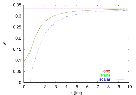
Figure 2: Spectral equations of state computed from Eqs. (12) and (17) as applied to the three constituting terms of the energy density and pressure.

Fig.2 displays the measured equations of state of the three types of fields. It is obvious that the longitudinal and the transverse gauge fields show degenerate behaviour despite of the rather different formal procedure of the determination of $w_{L}$ and $w_{T}$. The fitted squared masses appear in Table 2.

		Lagrangian mass squared		equipartition mass squared
$T_{kinetic}(|m|)$	$\epsilon_{total}(|m|^{4})$	scalar	trans & long	scalar	trans	long
0.0409	1.91	$1.80\pm 0.05$	$0.93\pm 0.02$	$2.16\pm 0.02$	$0.95\pm 0.01$	$0.92\pm 0.01$
0.0102	0.47	$1.95\pm 0.03$	$0.98\pm 0.01$	$2.23\pm 0.02$	$0.99\pm 0.02$	$0.98\pm 0.01$
0.0025	0.12	$1.99\pm 0.01$	$1.00\pm 0.00$	$2.26\pm 0.03$	$1.00\pm 0.02$	$0.99\pm 0.01$
0.0006	0.03	$2.00\pm 0.00$	$1.00\pm 0.00$	$2.26\pm 0.03$	$1.00\pm 0.03$	$1.00\pm 0.01$

Table 1: The comparison of the averaged mass terms of the Lagrangian (e.g. $M_{i}^{2}\varphi_{i}^{2},~{}~{}\varphi_{i}=\rho,{\bf A}_{T},{\bf A}_{L}$) with the thermodynamically fitted effective squared masses $M_{i,eff}^{2}$.

It is remarkable that for the Higgs field the measured values of the squared mass are 10-15% higher than expected on the basis of (20). This is the effect of the ultraviolet fluctuations which modify at one loop its mass [12] the following way:

$$M^{2}_{H,lattice}=m^{2}+\frac{\lambda}{2}\overline{\rho^{2}}+\left(3e^{2}+\frac{\lambda}{2}\right)\frac{0.226}{a^{2}}.$$ (21)

Indeed, the variation of the deviation from the tree level squared mass at very low energy densities was found to be inversely proportional to $a^{2}$. The non-perturbatively fitted coefficient is much smaller, than the 1-loop estimate appearing above. The convergence of the measured Higgs mass to a well-defined value for $T\approx 0$ makes it possible to define the renormalised Higgs mass. If one chooses it to coincide with the curvature of the classical potential at its minimum (e.g. (20)), then with the same subtraction one can define also the temperature dependent mass. In this way a very good agreement of the renormalised squared masses with the predicted temperature dependence was found.

The effective squared masses of the vector modes were found very close to $M^{2}_{V}=\overline{e^{2}\rho^{2}}$ without observable lattice spacing dependence.

3 The statistics of the elementary fields

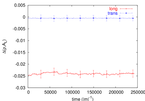
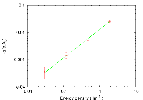
Figure 3: Correlation between the scalar field and the longitudinal and transversal gauge fields. On the left the binned averages of (22) are displayed as a function of time (measured in units $|m|^{-1}$). The error bars show the actual amplitude of its fluctuations. The average values of the correlation coefficients are shown in the right hand figure as a function of the energy density (measured in units $|m|^{4}$). The variation is compatible with the vanishing of the correlation for vanishing energy density (its slope is: $1.04\pm 0.04$).

In this section we shall analyse the data in further details focusing on the statistical correlations of the field variables $\rho,{\bf A}_{L},{\bf A}_{T}$. Our aim is to find the field-coordinates of the quasi-particles, emerging from the thermodynamical analysis of the previous section. There are two aspects of this search:

• Can one consider the above variables mutually independent in statistical sense?

• Do they follow Gaussian statistics expected for small amplitude, nearly free quasi-particle oscillations?

As a signature of independence of two field variables we shall consider the factorisability of the spatial average of their quadratic products by testing if, for instance,

$$\Delta[{\bf A}_{T},\rho]\equiv\frac{\overline{\rho^{2}({\bf x},t){\bf A}_{T}^{2}({\bf x},t)}-\overline{\rho^{2}({\bf x},t)}~{}\overline{{\bf A}_{T}^{2}({\bf x},t)}}{\overline{\rho^{2}({\bf x},t){\bf A}_{T}^{2}({\bf x},t)}}=0$$ (22)

is fullfilled (analoguous test is performed for $\Delta[{\bf A}_{L},\rho]$). For variables obeying Gaussian statistics the equality

$$\Gamma[{\bf A}_{T}]\equiv\frac{\overline{\left({\bf A}_{T}^{2}({\bf x},t)\right)^{2}}-3\left(\overline{{\bf A}_{T}^{2}({\bf x},t)}\right)^{2}}{\overline{\left({\bf A}_{T}^{2}({\bf x},t)\right)^{2}}}=0$$

is obeyed.

Clear quantitative evidence appears on the left hand side of Fig.3 for the stationary (time-independent) independence of ${\bf A}_{T}$ and $\rho$. On the other hand ${\bf A}_{L}$ and $\rho$ show non-zero correlation, which appears also constant in time. The test of Gaussianity shows that from very early times both $\Gamma[{\bf A}_{T}]$ and $\Gamma[\rho]$ vanish, while $\Gamma[{\bf A}_{L}]$ violates the criterium concerning the Gaussian nature of its statistics.

On the right hand side of Fig. 3 we give the dependence of $\Delta[{\bf A}_{L},\rho]$ on the average energy density of the system. (The corresponding temperatures, understood in the sense described in section 2, are listed in Table 1). The effect increases linearly with the energy density. Analogous behaviour is observed for $\Gamma[{\bf\Pi}_{L}]$ and $\Delta[{\bf\Pi}_{L},\rho]$, where ${\bf\Pi}_{L}$ is the canonical momentum field conjugate to ${\bf A}_{L}$. The correlation coefficient $\Delta({\bf A}_{L},\rho)$ was computed also on lattices of the same physical size but smaller lattice spacing providing essentially the same result. The lack of the $\rho-{\bf A}_{L}$ factorisation was demonstrated on a number of functions $f(\rho)$ replacing $\rho^{2}$, among them also $(\rho-\overline{\rho})^{2}$.

In systems with large values of the couplings this strong correlation could be natural to expect. In this respect it is more surprising that the transversal gauge field behaves as a perfect independent variable. In non-equilibrium time evolution, when in addition to the small amplitude white noise initial conditions applied to the ${\bf k}\neq 0$ modes, the average Higgs field (${\bf k}=0$) starts from the unstable maximum at $\overline{\rho}=0$ we have observed frequently the generation of rather large nonzero values for $\Delta[{\bf A}_{T},\rho]$. Some spectacular examples are presented in Fig.4. One observes a rather abrupt vanishing of these values after certain time elapses. It turns out that in case of the transverse fields nonzero quasi-stationary values of $\Delta[{\bf A}_{T},\rho]$ are very sensitive indicators of the presence of Nielsen-Olesen vortex-antivortex pairs [23]. A representative vortex-antivortex pair is displayed in the right hand figure of Fig.4. The drop of the absolute value of $\Delta[{\bf A}_{T},\rho]$ occurs when the pair annihilates. Similar, but less pronounced drop is observed in the correlation of the Higgs field and the magnetic plaquette variable, which is strictly gauge invariant even for finite lattice spacing. It is clear that in the vortex solution presented in [23] the transversal vector potential and the real Higgs field vary in a correlated way. The detailed statistics of the vortex production during spinodal instability will be discussed in a separate publication. Here we conclude as a byproduct from this analysis, that the vanishing of $\Delta[{\bf A}_{T},\rho]$ in equilibrium not only hints to the independence of the ${\bf A}_{T}$-statistics, but also represents evidence that no vortex lines are present in our equilibrium configurations.

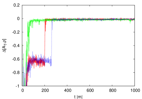
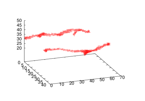
Figure 4: Left: Three examples of the non-equilibrium evolution of $\Delta[{\bf A}_{T},\rho]$. In two time-histories stationary nonzero values of $\approx-0.6$ occured for a restricted time interval. It signals the presence of a vortex-antivortex pair and can be easily distinguished from the fast and smooth relaxation to zero, when no vortices are generated. Right: The vortex-antivortex pair corresponding to non-zero $\Delta$, is found by looking for the points where $\rho<0.3$

We have investigated also the dependence of $\Delta[{\bf A}_{L},\rho]$ and $\Delta[{\bf A}_{T},\rho]$ on the Higgs-gauge mass ratio, that is on $\lambda/e^{2}$. The value of $\lambda$ was varied in the range $(0.75,75)$ keeping the energy density fixed and $e^{2}=1$. $\Delta[{\bf A}_{L},\rho]$ linearly increases from $\sim 0.001$ up to $\sim 0.1$. Specifically, no effect on this linear variation can be observed when the decay channel of the Higgs into two ”photons” opens around $\lambda/e^{2}\sim 12$. The time average of $\Delta[{\bf A}_{T},\rho]$ stays zero, only the size of its fluctuations increases. We have checked that the correlative effects do not change for $e^{2}=0.01$.

In concluding this section we elaborate on the consequences of the statistical independence of ${\bf A}_{T}$ and $\rho$ on the thermodynamics. The Gaussian nature of the Fourier modes of ${\bf A}_{T}$ is expressed by the following formula:

$$\overline{{\bf A}_{T}({\bf k}){\bf A}^{*}_{T}({\bf k}^{\prime})}=\overline{|{\bf A}_{T}({\bf k})|^{2}}\delta_{{\bf k},{\bf k}^{\prime}}.$$ (23)

Let us apply it to the statistical expectation of a weighted space-average of ${\bf A}_{T}({\bf x})$. One can make the observation that both $\epsilon_{T}$ and $p_{T}$ are quadratic expressions of ${\bf A}_{T}$, multiplied by some function of $\rho$. First one substitutes for ${\bf A}_{T}$ its Fourier expansion. When the independence of the ${\bf A}_{T}$ statistics from $\rho$ is used, the average can be written in a factorized way. Finally, (23) is used and provides a simple general formula:

$$\overline{\frac{1}{V}\int d^{3}xf[\rho({\bf x},t)]{\bf A}_{T}^{2}({\bf x},t)} = \overline{\frac{1}{V}\int d^{3}xf[\rho({\bf x},t)]\sum_{{\bf k},{\bf k}^{\prime}}e^{i({\bf k}-{\bf k}^{\prime}){\bf x}}~{}}\times\overline{{\bf A}_{T}({\bf k},t){\bf A}_{T}^{*}({\bf k}^{\prime},t)}$$ (24)

$$= \overline{\langle f[\rho({\bf x},t)]\rangle_{V}}\sum_{\bf k}\overline{|{\bf A}_{T}({\bf k},t)|^{2}},$$

where the bracket with lower index $V$ was introduced to denote the spatial averaging. This representation allows for the following identification of the corresponding spectral density, with no ambiguity left in its definition:

$$\overline{\langle f[\rho]{\bf A}^{2}\rangle_{V}}({\bf k})\equiv\overline{\langle f[\rho({\bf x},t)]\rangle_{V}}~{}\overline{|{\bf A}({\bf k},t)|^{2}}.$$ (25)

Direct consequences of this are the following expressions for $\overline{\epsilon}_{T},\overline{p}_{T}$, where factorized averaging over ${\bf A}_{T}$ and $\rho$ appears:

$$\overline{\epsilon_{T}}({\bf k}) = \frac{1}{2}\left[\overline{|{\bf\Pi}_{T}({\bf k})|^{2}}+({\bf k}^{2}+\overline{\langle e^{2}\rho^{2}\rangle_{V}})\overline{|{\bf A}_{T}({\bf k})|^{2}}\right],$$

$$\overline{p_{T}}({\bf k}) = \frac{1}{6}\left[\overline{|{\bf\Pi}_{T}({\bf k})|^{2}}+({\bf k}^{2}-\overline{\langle e^{2}\rho^{2}\rangle_{V}})\overline{|{\bf A}_{T}({\bf k})|^{2}}\right].$$ (26)

They are equivalently given through the expression of the dispersion relation and the equation of state of the transversal quasi-particles:

$$\omega_{T}^{2}({\bf k})=\frac{\overline{|{\bf\Pi}_{T}({\bf k})|^{2}}}{\overline{|{\bf A}_{T}({\bf k})|^{2}}}={\bf k}^{2}+\overline{\langle e^{2}\rho^{2}\rangle_{V}},\qquad w_{T}({\bf k})\equiv\frac{\overline{p}_{T}({\bf k})}{\overline{\epsilon}_{T}({\bf k})}=\frac{1}{3}\frac{{\bf k}^{2}}{{\bf k}^{2}+\overline{\langle e^{2}\rho^{2}\rangle_{V}}}.$$ (27)

(The dispersion relation emerges from the average kinetic-potential energy equality for each mode). These expressions reproduce perfectly the original transversal spectral densities and the EoS extracted in the previous section.

Similarly good representation is obtained for the thermodynamics of the Higgs-sector when the Gaussianity of $\rho$ is imposed on the averaging. In case of ${\bf A}_{L}$ a very bad quality representation of the spectral equation of state is possible if independence and Gaussianity are forced upon the longitudinal part of the vector potential. The quality of the description can be characterized by the violation of the kinetic-potential energy equality (18), which is displayed in Fig.6.

Since the characteristics of the longitudinal equation of state clearly possess a quasi-particle character, as was seen in section 2, our conclusion is that ${\bf A}_{L}$ cannot be the corresponding quasi-particle coordinate. Instead in the next section we search for an appropriate non-linear combination of ${\bf A}_{L}$ and $\rho$.

4 Search for the longitudinal quasi-particle

We search for nonlinear combinations of the longitudinal vector potential and $\rho$ for which in (22) and (3) equalities can be verified. This should support the general view of almost free quasi-particle composition of finite temperature media. It should be checked whether for this new combination the equipartition and the spectral equation of state can be interpreted consistently under the assumption of the factorisation of their statistics. It will be also checked to what extent it follows Gaussian statistics. Eventually we show that the quality of the equation of state based on this independent new variable is almost as good as the result of Section 2. We shall work out the example of (1), and only comment on the performance of the alternative proposition (2).

The coefficient $\alpha$ in (1) could be estimated analytically by assuming that it is small. For a quantitative treatment there is no need to apply approximations. By tuning $\alpha$ continuously we have measured the normalised reduced correlation functions $\Delta({\cal A}_{L},\rho)$ and $\Delta({\cal P}_{L},\rho)$. In Fig. 5 these two curves are displayed as functions of $\alpha$ together with the quantities testing the Gaussian nature of the new variables. It is remarkable that both the new coordinate and its conjugate momentum become uncorrelated with the Higgs-field for the same $\alpha$. Although they are not perfect Gaussian variables, the deviation from Gaussianity is minimal just for this $\alpha$ value, it is about 5 times smaller than at $\alpha=0$. The situation is very similar for the nonlinear mapping (2) as can be seen from the twin figure of Fig. 5. It is important to notice that in the latter case $\alpha\neq 1$, which would be the naive expectation on the basis of the way the kinetic-potential equipartition is fulfilled. Further in the analysis we use the optimal $\alpha$ values found as the average over 40 independent configurations. It has to be emphasised that no unique $\alpha_{opt}$ exists for single configurations, the optimal values found from the four different criteria fluctuate somewhat. It is the ensemble average which leads to the remarkable coincidence displayed in Fig. 5.

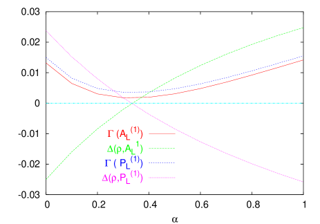
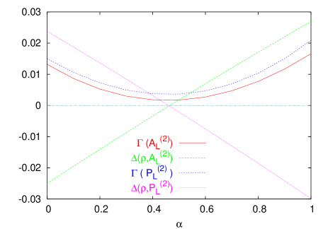
Figure 5: Correlators of two versions of the nonlinearly mapped ”longitudinal” field as a function of the parameter $\alpha$. On the left the results of the mapping (1), on the right the mapping (2) are shown.

Now one has to reexpress the partial energy densities and pressures in terms of the new variables. One should not forget that as a consequence of (1) also the canonical momentum conjugate to $\rho$ changes:

$${\cal P}_{\rho}+\frac{2\alpha\rho}{1+\alpha\rho^{2}}{\cal A}_{L}{\cal P}_{L}={\bf\Pi}_{\rho}$$ (28)

Assuming factorisation of the statistical averaging over $\rho,\Pi_{\rho}$ and ${\cal A}_{L},{\cal P}_{L}$ one obtains the following expressions for the averaged energy densities:

$$\overline{\epsilon}_{\rho} = \frac{1}{2}\overline{{\cal P}_{\rho}^{2}}+\overline{\frac{2\alpha^{2}\rho^{2}}{3(1+\alpha\rho^{2})^{2}}}\overline{{\cal A}_{L}^{2}}~{}\overline{{\cal P}_{L}^{2}}+\frac{1}{2}\overline{(\nabla\rho)^{2}}+\frac{1}{2}M_{eff}^{2}\overline{\rho^{2}},$$

$$\overline{\epsilon}_{L} = \frac{1}{2}\left(\overline{(1+\alpha\rho^{2})^{2}}+\overline{\frac{(\alpha\nabla\rho^{2})^{2}}{e^{2}\rho^{2}}}\right)\overline{{\cal P}_{L}^{2}}+\frac{1}{2}\overline{\frac{(1+\alpha\rho^{2})^{2}}{e^{2}\rho^{2}}}\overline{(\nabla{\cal P}_{L})^{2}}$$ (29)

$$+ \frac{1}{2}\overline{\frac{e^{2}\rho^{2}}{(1+\alpha\rho^{2})^{2}}}\overline{{\cal A}_{L}^{2}}.$$

It is worth now to check if the equality between the first two and the last term of Eq.(29) is fullfilled in the present factorised form. Fig. 6 demonstrates no more than 1% deviation from the almost perfect equality found in Section 2.

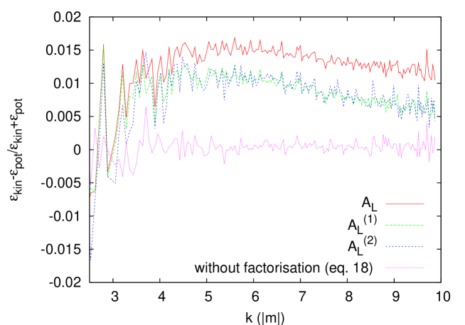
Figure 6: The quality of the mode-by-mode equality of the longitudinal kinetic and potential energies when i) the original ${\bf A}_{L}$, ii) the nonlinearly constructed variable ${\cal A}_{L}^{(i)}$ are proposed as statistically independent fields. For comparison the perfect fullfillment of (18) is also presented . The region $k\geq 2|m|$ is shown, where the equipartition is very well fullfilled for the other degrees of freedom.

The corresponding expressions for the partial pressures are as follows:

$$\overline{p}_{\rho} = \frac{1}{2}\overline{{\cal P}_{\rho}^{2}}+\overline{\frac{2\alpha^{2}\rho^{2}}{3(1+\alpha\rho^{2})^{2}}}\overline{{\cal A}_{L}^{2}}~{}\overline{{\cal P}_{L}^{2}}-\frac{1}{6}\overline{(\nabla\rho)^{2}}-\frac{1}{2}M_{eff}^{2}\overline{\rho^{2}},$$

$$\overline{p}_{L} = \frac{1}{6}\left(\overline{(1+\alpha\rho^{2})^{2}}~{}\overline{{\cal P}_{L}^{2}}-\overline{\frac{e^{2}\rho^{2}}{(1+\alpha\rho^{2})^{2}}}\overline{{\cal A}_{L}^{2}}\right)$$ (30)

$$+ \frac{1}{2}\overline{\frac{(\alpha\nabla\rho^{2})^{2}}{e^{2}\rho^{2}}}\overline{{\cal P}_{L}^{2}}+\frac{1}{2}\overline{\frac{(1+\alpha\rho^{2})^{2}}{e^{2}\rho^{2}}}\overline{(\nabla{\cal P}_{L})^{2}}.$$

It is worth to write explicitly the spectral equation of state resulting for the new effective field variables, when the improved but still approximate equipartition is exploited:

$$w_{new}(k)=\frac{1}{3}\frac{\overline{\frac{(\alpha\nabla\rho^{2})^{2}}{e^{2}\rho^{2}}}+{\bf k}^{2}\overline{\frac{(1+\alpha\rho^{2})^{2}}{e^{2}\rho^{2}}}}{\overline{(1+\alpha\rho^{2})^{2}}+\overline{\frac{(\alpha\nabla\rho^{2})^{2}}{e^{2}\rho^{2}}}+{\bf k}^{2}\overline{\frac{(1+\alpha\rho^{2})^{2}}{e^{2}\rho^{2}}}}.$$ (31)

The correction in the energy density and the pressure of $\rho$ turns out to be negligible. In Fig. 7 we plot the ”longitudinal” equation of state using (29) and (30), by measuring the corresponding averages directly, and the ”theoretical” curve (31). A rather remarkable agreement of the curves is seen which works the best for low and moderate values of $k$. The systematic deviation experienced in the high $k$ region would require smaller mass, which however would lead to large discrepancy in the low $k$ region. Similar features are observed when the equation of state is constructed with help of the mapping (2). The curve corresponding to (31) agrees very well with the longitudinal equation of state appearing in Fig. 2.

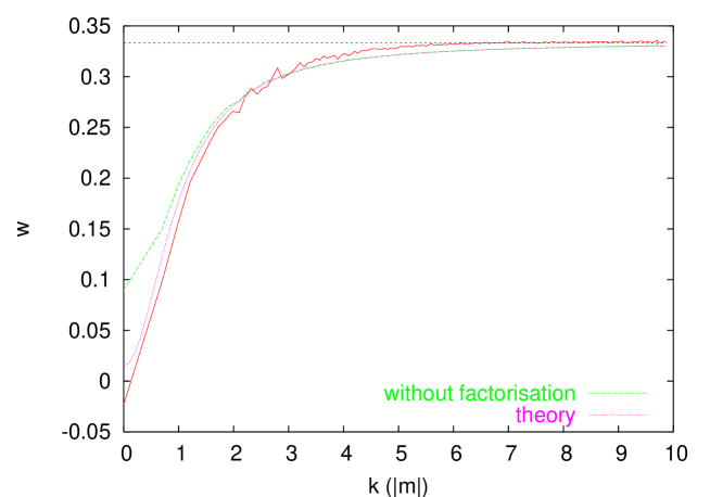
Figure 7: Sperctral equation of state with ${\bf{\cal A}}_{L}^{(1)}$ (continuous line) as compared with the curve (31) (”theory”, dotted line) where the $\rho$ dependence of the coefficients is averaged numerically. The equation of state obtained in Section 2 (”without factorisation”, dashed line) is also shown for comparison.

5 Conclusions

In the present investigation we searched for the quasi-particles of the classical Abelian Higgs model at finite (low) energy density. The validity of a quasi-particle representation of the thermodynamics is essential for cosmological applications. The intuitively expected statistical independence and Gaussian behaviour of the transversal gauge field and of the Higgs excitations in the unitary gauge was confirmed.

The longitudinal component of the vector field is not independent statistically at finite energy density from the Higgs oscillations. This correlation and the deviation from the Gaussian statistics grows with the temperature and also with the $\lambda/e^{2}$ ratio. Still, its thermodynamical characteristics represented in form of a spectral equation of state were shown to be degenerate with the features of the transverse vector modes.

The first step of the search for an independent Gaussian pair of canonically conjugate field variables describing the non-transversal gauge fluctuations was put forward in this paper. We are confident that a fourth quasi-particle degree of freedom completes the thermodynamical characterisation, though there is no unique prescription for its systematical construction. One possibility is to abandon the idea of a local mapping in ${\bf x}$-space and try to use a ${\bf k}$-dependent mixing parameter: $\alpha({\bf k})$.

The present experience is very useful also for the investigation of the real time evolution of the field excitations in an inflaton+Gauge+Higgs system starting from an unstable (symmetric) initial state and ending in the broken symmetry phase. We are interested in the rate of excitation of the different field degrees of freedom immediately after the exit from inflation. Already at present it is clear that vortex-antivortex pair production will be rather frequent and can be studied also with help of the correlation coefficients introduced in the present study. It will be interesting to see whether the energy transfer from the inflaton to the quasi-particles related to the transverse and the longitudinal vector fields is symmetrical. These questions are under current investigation.

Appendix

The thermal equilibrium of the system was realised in our real time simulations by long temporal evolution. It started from a noisy initial state having finite energy density. In order to implement the equations of motion in the temporal axial gauge, a spatial lattice was introduced. On this lattice the gauge field and the covariant (forward, $F$) derivatives of the scalar field are approximated with help of link variables:

$$U_{i}(x)=e^{-ie|a_{i}|A_{i}(x)},\quad D_{i}^{F}\Phi(x)=\frac{1}{|a_{i}|}\left(U_{i}(x)\Phi(x+a_{i})-\Phi(x)\right).$$ (32)

The compact nature of $U$’s has no effect at very low energy densities studied in the persent investigation. The solution of the equations of motion was started with all conjugate momenta set to zero. Under this condition the Gauss constraint is trivially fulfilled in the temporal axial gauge and it is preserved during the evolution. The Fourier modes of the canonical coordinate fields were given an amplitude with random phase, providing for each mode equal potential energy. The simulations were done mostly on $N=32$ three-dimensional lattices with a lattice constant $a=0.35|m|^{-1}$. In order to test the possible lattice constant dependence of the effects the system was solved also on $N=64,a=0.174|m|^{-1}$ lattice. Notable lattice spacing dependence was observed only for the Higgs mass (see the main discussion).

The vector potential and its conjugate momenta are computed on an isotropic lattice $(a_{i}=a)$ as

$$A_{i}(x)=-\frac{1}{ea}{\rm Im}U_{i}(x),\quad\Pi_{i}=\frac{1}{ea\delta t}{\rm Im}\left(U_{i}(x+a\delta t)U^{-1}_{i}(x)\right),$$ (33)

where the discrete time-step we use is $a_{0}=a\delta t$ with $\delta t\sim 0.1$. These fields were decomposed into tranverse and longitudinal components, we need in the formulae for the decomposition of the energy and pressure. The magnetic field strength is measured from the plaquette variables

$$U_{ij} = U_{j}^{-1}(x)U_{i}^{-1}(x+a_{j})U_{j}(x+a_{i})U_{i}(x),$$

$${\rm Im}U_{ij} = -ea^{2}\epsilon_{ijk}B_{k}.$$ (34)

In the moments of measurements the actual configuration was transformed to unitary gauge.

Acknowledgements

The authors are grateful to J. Smit for valuable suggestions. Enjoyable discussions with Sz. Borsányi, A. Jakovác and P. Petreczky are also acknowledged. This research was supported by the Hungarian Research Fund (OTKA), contract No. T-037689.

References

- [1] P.W. Higgs, Phys. Rev. Lett. 13 (1964) 508
- [2] P.W. Higgs, Phys. Rev. 145 (1966) 1156
- [3] H.G. Evertz, J. Jersák, C.B. Lang and T. Neuhaus, Phys. Lett. B171 (1986) 271
- [4] F. Csikor, Z. Fodor, J. Hein, A. Jaster and I. Montvay, Nucl. Phys. 474 (1996) 421
- [5] F. Csikor, Z. Fodor and J. Heitger, Phys. Rev. Lett. 82 (1999) 21
- [6] J. Ambjorn, T. Askgaard, H. Porter and M. Shaposhnikov, Nucl. Phys. B353 (1991) 346
- [7] G.D. Moore, Phys. Rev. D59 (1999) 014503
- [8] M. Hindmarsh and A. Rajantie, Phys. Rev. D64 (2001) 065016
- [9] J.N. Moore, E.P.S. Shellard and C.J.A.P. Martins, Phys. Rev. D65 (2001) 023503
- [10] J. Garcia-Bellido, M. Garcia Perez and A. Gonzalez-Arroyo, Phys. Rev. D69 (2004) 023504
- [11] J. Garcia-Bellido, D. Grigoriev, A. Kusenko and M. Shaposhnikov, Phys. Rev. D60 (1999) 123504
- [12] A. Rajantie, P.M. Saffin and E.J. Copeland, Phys. Rev. D63 (2001) 123512
- [13] E.J. Copeland, S. Pascoli and A. Rajantie, Phys. Rev. D65 (2002) 103517
- [14] T.Asaka, D.Grigoriev, V. Kuzmin and M. Shaposhnikov, Phys. Rev. Lett. 92 (2004) 101303
- [15] A.Tranberg and J. Smit, JHEP 0311 (2003) 016
- [16] A.D. Linde, Phys. Rev. D49 (1994) 748
- [17] L. Kofman, A.D. Linde and A.A. Starobinsky, Phys. Rev. D56 (1997) 3258
- [18] G.N. Felder, L. Kofman and A.D. Linde, Phys. Rev. D64 (2001) 123517
- [19] Sz. Borsányi, A. Patkós and D. Sexty, Phys. Rev. D68 (2003) 063512
- [20] J.-I. Skullerud, J. Smit and A. Tranberg, JHEP 0308 (2003) 045
- [21] Sz. Borsányi, A. Patkós and D. Sexty, Phys. Rev. D66 (2002) 025014
- [22] J. Berges, Sz. Borsányi and C. Wetterich, Phys. Rev. Lett. 93 (2004) 142002
- [23] H.B. Nielsen and P. Olesen, Nucl. Phys. B61 (1973) 45