BUHEP-05-1
hep-ph/0501204

Accidental Goldstone Bosons

Abstract

We study vacuum alignment in theories in which the chiral symmetry of a set of massless fermions is both spontaneously and explicitly broken. We find that transitions occur between different phases of the fermions’ CP symmetry as parameters in their symmetry breaking Hamiltonian are varied. We identify a new phase that we call pseudoCP-conserving. We observe first and second-order transitions between the various phases. At a second-order (and possibly first-order) transition a pseudoGoldstone boson becomes massless as a consequence of a spontaneous change in the discrete, but not the continuous, symmetry of the ground state. We relate the masslessness of these “accidental Goldstone bosons” (AGBs) bosons to singularities of the order parameter for the phase transition. The relative frequency of CP-phase transitions makes it commonplace for the AGBs to be light, much lighter than their underlying strong interaction scale. We investigate the AGBs’ potential for serving as light composite Higgs bosons by studying their vacuum expectation values, finding promising results: AGB vevs are also often much less than their strong scale.

I. Introduction

In this paper we describe phenomena we believe to be very general but which appear to have received almost no attention in particle physics. These are the presence of various phases of CP symmetry, of transitions among these phases, and of anomalously light bosons which become massless at these phase transitions. While, in the model calculations we present, the massless state is a pseudoGoldstone boson (PGB) of an approximate chiral symmetry, the boson’s masslessness is not due to the restoration of its associated continuous chiral symmetry. Rather, it is due to a change in the phase of the discrete CP symmetry. Following Dashen, who first observed this phenomenon in the context of QCD, we call these “accidental Goldstone bosons” (AGBs). Unlike Dashen, however, we do not believe the AGB’s mass necessarily is restored by higher-order corrections. Rather, we suspect that corrections only shift the values of parameters at which phase transitions occur.

This study grew out of earlier work on vacuum alignment in technicolor theories of dynamical electroweak symmetry breaking [2, 3]; also see Ref. [4] for a recent summary. However, although our calculations are similar to those used in technicolor, we are confident our conclusions extend beyond that setting. Some of the phenomena we observe also occur in QCD when one allows an odd number of real quark masses to become negative (so that $\bar{\theta}=\pi$) [1, 5]). We see no reason they would not also occur in models different from the type we investigate here. They may even have relevance to condensed matter systems.

The model we use assumes $N$ massless Dirac fermions $T_{i}=(T_{Li},T_{Ri})$, $i=1,\dots,N$, transforming according to a complex representation of a strongly-coupled $SU(N_{c})$ gauge group. The fermions’ chiral flavor symmetry, $G_{f}=SU(N)_{L}\otimes SU(N)_{R}$, is spontaneously broken to an $SU(N)$ subgroup. It is convenient to work in a “standard vacuum” $|\Omega\rangle$ whose symmetry is the vectorial $S_{f}=SU(N)_{V}$ defined by the $SU(N_{c})$-invariant condensates

$$\langle\Omega|\bar{T}_{Li}T_{Rj}|\Omega\rangle=\langle\Omega|\bar{T}_{Ri}T_{Lj}|\Omega\rangle=-\delta_{ij}\Delta_{T}\,.$$ (1)

The condensate $\Delta_{T}$ is renormalized at the $SU(N_{c})$ scale $\Lambda_{T}$, which (for $T_{i}\in{\boldsymbol{N}_{c}}$ of $SU(N_{c})$) is commonly assumed to be $\Lambda_{T}\simeq 4\pi F_{\pi}$ and, then, $\Delta_{T}\simeq 2\pi F^{3}_{\pi}$. Here, $F_{\pi}$ is the decay constant of the massless Goldstone bosons, $\pi_{a}$, $a=1,\dots,N^{2}-1$, resulting from the spontaneous chiral symmetry breaking. It is normalized by the relation $\langle\Omega|\bar{T}\gamma_{\mu}\gamma_{5}t_{a}T|\pi_{b}(p)\rangle=iF_{\pi}p_{\mu}\delta_{ab}$, with $t_{a}=\lambda_{a}/2$ so that ${\rm Tr}(t_{a}t_{b})=\frac{1}{2}\delta_{ab}$.

The chiral $SU(N)_{L}\otimes SU(N)_{R}$ symmetry is also broken explicitly by the $SU(N_{c})$-invariant four-fermion interactions

$${\cal H}^{\prime}=\sum_{ijkl}\Lambda_{ijkl}\bar{T}_{Li}\gamma^{\mu}T_{Lj}\bar{T}_{Rk}\gamma_{\mu}T_{Rl}+{\rm LL\,,\,RR\,\,\,terms}+{\rm h.c.}\,,$$ (2)

where the unexhibited LL and RR terms are irrelevant for our further discussion. The $\Lambda_{ijkl}=\Lambda^{*}_{jilk}$ are inverse squared masses of gauge bosons (or scalars) exchanged between the “currents” (or their Fierz transforms) in ${\cal H}^{\prime}$. They are chosen in numerical calculations so that all $\pi_{a}$-symmetries are explicitly broken. Ordinarily, then, we would expect the PGBs to acquire positive mass-squared. Finally, we assume that ${\cal H}^{\prime}$ is T-invariant, i.e.,

$$\Lambda_{ijkl}=\Lambda^{*}_{ijkl}\,.$$ (3)

Now, there may be a mismatch between the standard vacuum $|\Omega\rangle$ and the one in which ${\cal H}^{\prime}$ of Eq. (2) gives positive mass-squared to all $\pi_{a}$. It is therefore necessary to “align the vacuum”, more precisely, to determine the correct ground state $|{\rm vac}\rangle$ of the theory [1]. In this state, $\langle{\rm vac}|{\cal W}^{-1}{\cal H}^{\prime}{\cal W}|{\rm vac}\rangle$, varied over ${\cal W}\in SU(N)_{L}\otimes SU(N)_{R})$, is a minimum at ${\cal W}=1$. We follow Dashen’s procedure, which is based on lowest-order chiral perturbation theory and minimize the vacuum energy defined over the infinity of perturbative ground states $|\Omega({\cal W})\rangle$:

$$E(W) = \langle\Omega({\cal W})|{\cal H}^{\prime}|\Omega({\cal W})\rangle\equiv\langle\Omega|{\cal W}^{-1}{\cal H}^{\prime}{\cal W}|\Omega\rangle$$ (4)

$$= -\sum_{ijkl}\Lambda_{ijkl}W_{jk}W^{\dagger}_{li}\Delta_{TT}+{\rm constant}\,.$$

Here, we used (since $T_{L,R\,i}$ transform as a complex representation of $SU(N_{c})$)

$$\langle\Omega|\bar{T}_{Li}\gamma^{\mu}T_{Lj}\bar{T}_{Rk}\gamma_{\mu}T_{Rl}|\Omega\rangle=-\delta_{il}\delta_{jk}\Delta_{TT}\,.$$ (5)

Since $|\Omega\rangle$ is invariant under $SU(N)_{V}$ transformations, the $SU(N)$ matrix $W=W_{L}W_{R}^{\dagger}\in G_{f}/S_{f}$ is the only physically meaningful combination of $W_{L}$ and $W_{R}$. The four-fermion condensate is renormalized at the scale of the exchanged-boson masses making up the $\Lambda_{ijkl}$. This scale is likely to be much greater than $\Lambda_{T}$. In a QCD-like $SU(N_{c})$ theory, $\Delta_{TT}\sim\Delta_{T}^{2}$. If $SU(N_{c})$ is a walking gauge theory [6, 7, 8, 9], $\Delta_{TT}$ could be much larger than $\Delta_{T}^{2}$, partially overcoming the suppression by the $\Lambda_{ijkl}$.

Note that CP-invariance of ${\cal H}^{\prime}$ implies that $E(W)=E(W^{*})$. The $W_{0}$ which minimizes $E$ is defined up to a factor $Z_{N}^{m}=\exp{(2im\pi/N)}$, $m=0,\dots,N-1$. If, apart from this trivial ambiguity, $W_{0}\neq W_{0}^{*}$, then the correct chiral-perturbative ground state is discretely degenerate and CP symmetry is spontaneously broken. Equivalently, and more conveniently, the Hamiltonian ${\cal H}^{\prime}({\cal W}_{0})={\cal W}_{0}^{-1}{\cal H}^{\prime}\,{\cal W}_{0}$ correctly aligned with the standard $|\Omega\rangle$ violates CP.

It is convenient to make the $SU(N)_{V}$ transformation $W_{L,R}\rightarrow W_{L,R}W^{\dagger}_{R}$. This amounts to computing ${\cal H}^{\prime}({\cal W}_{0})$ with $W_{L}=W$, $W_{R}=1$. Then, dropping the subscript “0” from now on,

$${\cal H}^{\prime}(W) = \sum_{ijkl}\Lambda^{W}_{ijkl}\bar{T}_{Li}\gamma^{\mu}T_{Lj}\bar{T}_{Rk}\gamma_{\mu}T_{Rl}+{\rm LL\,,\,RR\,\,\,terms}+{\rm h.c.}\,,$$

$$\Lambda^{W}_{ijkl} = \sum_{i^{\prime},j^{\prime}}\Lambda_{i^{\prime}j^{\prime}kl}W^{\dagger}_{ii^{\prime}}W_{j^{\prime}j}\,.$$ (6)

After this vectorial transformation, the PGB mass-squared matrix is still calculated using the axial charges, formally defined by $Q_{5a}=\int d^{3}x\,T^{\dagger}\gamma_{5}t_{a}T$. To lowest order in chiral perturbation theory [10],

$$F_{\pi}^{2}M^{2}_{ab}=i^{2}\left\langle\Omega\left|\left[Q_{5a},\left[Q_{5b},{\cal H}^{\prime}(W)\right]\right]\right|\Omega\right\rangle\,.$$ (7)

For the Hamiltonian in Eq. (I. Introduction).

$$F_{\pi}^{2}M^{2}_{ab} = 2\sum_{ijkl}\Lambda_{ijkl}\Bigl{[}\left(\left\{t_{a},t_{b}\right\}W^{\dagger}\right)_{li}\,W_{jk}+W_{li}^{\dagger}\,\left(W\left\{t_{a},t_{b}\right\}\right)_{jk}$$ (8)

$$\qquad-2\left(t_{a}W^{\dagger}\right)_{li}\,\left(Wt_{b}\right)_{jk}-2\left(t_{b}W^{\dagger}\right)_{li}\,\left(Wt_{a}\right)_{jk}\thinspace\Bigr{]}\Delta_{TT}\,.$$

Finally, it is very useful to parameterize $W$ in the form

$$W=D_{L}KD_{R}\thinspace.$$ (9)

Here, $D_{L,R}$ are diagonal $SU(N)$ matrices, each involving $N-1$ independent phases $\chi_{L,R\,i}$, and $K$ is an $(N-1)^{2}$–parameter CKM matrix which may be written in the standard Harari-Leurer form [11].

The remainder of this paper is organized as follows: In Sec. II we review vacuum alignment for the model we’ve described. The four-fermion form of ${\cal H}^{\prime}$ implies a linking of the phases in $W$ which allows the possibility of three “phase phases” with different CP properties. We call these three phases CP-conserving (CPC), pseudoCP-conserving (PCP), and CP-violating (CPV). In the CPC phase, $W$ is $Z_{N}^{m}$ times a real matrix and ${\cal H}^{\prime}(W)$ is real. In the PCP phase, $W$ is not simply $Z_{N}^{m}$ times a real matrix, but the phases in $W$ are rational multiples of $\pi$ and the CKM matrix $K$ is real. The phases in ${\cal H}^{\prime}(W)$ are also rational, but the Hamiltonian is not merely real up to an overall phase. However, introducing the aligning matrix $\widehat{W}=D_{R}WD_{R}^{\dagger}=D_{R}D_{L}K$, we show that the LR terms in ${\cal H}^{\prime}(\widehat{W})$ are real, i.e., CP-conserving, in both the CPC and PCP phases. In the CPV phase, the phases of $W$ are not rational multiples of $\pi$, $K$ is not real, and ${\cal H}^{\prime}(W)$ is definitely CP-violating.

We carry out vacuum alignment numerically in a three-flavor ($SU(3)$) model, varying one $\Lambda_{ijkl}\equiv\Lambda$ in ${\cal H}^{\prime}$. We observe each of these CP phases and note that the transitions between them are either first or second order — defined here as whether the first or second derivative of $E(W)$ with $\Lambda$ is discontinuous. Although we are varying just one of the parameters in ${\cal H}^{\prime}$, it is obvious that the phase transitions occur on surfaces in the space of $\Lambda_{ijkl}$’s. Our calculations are merely along a single trajectory in this $\Lambda$-space. There are two PGBs whose $M^{2}$ is much less than those of the other six. These are the accidental Goldstone bosons of this model. At all second-order (and, apparently, first-order) transitions one of these light PGBs becomes massless. We explain why this happens. Our calculations indicate that light AGBs are commonplace, at least as long as the $\Lambda_{ijkl}$ are the same order of magnitude. Then, competition among the $\Lambda$’s means that one is never very far from a CP phase transition and a surface in $\Lambda$-space on which an AGB mass vanishes.

Sections III and IV are devoted to understanding the phase transitions in more depth. In Sec. III we present a remarkable formula for $d^{2}E(W)/d\Lambda^{2}$ which connects the vanishing of $M^{2}$ to singular behavior of the “diagonal phases” of $W$, the $N-1$ phases $\omega_{Da}$, $a=n^{2}-1=3,8,\dots,N^{2}-1$, of $W$ in its diagonal form. This formula also directly relates the AGBs to the diagonal phases. The formula is derived in Appendix A. An analytic example of how it works is given in Appendix B using Dashen’s model — three quarks with negative masses. We also illustrate it numerically for the $SU(3)$ model. In Sec. IV we focus on the aligning matrix $\widehat{W}$. In the CPC and in what we call PCP-1 phases, $\widehat{W}=e^{im\pi/N}\widetilde{W}$ where $\widetilde{W}$ is real. In PCP-2 phases, $\widehat{W}$ cannot be written this way. In the CPC phase of the $SU(3)$ model we study, $\widetilde{W}$ appears to be symmetric. It is shown that this implies the normalized diagonal phases $\widehat{\omega}_{Da}=\omega_{Da}/\sqrt{n(n-1)/2}$ are rational multiples of $\pi$. In PCP-1 phases, $\widetilde{W}$ is not symmetric. In this case, some but not all the $\widehat{\omega}_{Da}$ are rational. We spell out the conditions for determining how many $\widehat{\omega}_{Da}$ are rational. In the PCP-2 phase, none of the $\widehat{\omega}_{Da}$ are rational. This is startling since all the phases in $W$ are.

Finally, in Sec. V we discuss one potential application of AGBs: light composite Higgs bosons for electroweak symmetry breaking [12, 13]. A light composite Higgs boson is a bound state whose mass and vacuum expectation value (vev) are naturally much less than the energy scale at which its binding occurs. The effort to construct realistic models of light composite Higgses has been driven by the strong experimental evidence in favor of the standard model with a light Higgs boson. Recently, much of this effort has focused on the little Higgs scenario [14, 15, 16, 17]. Little Higgs bosons are PGBs that are anomalously light because interlocking continuous symmetries need to be broken by several weakly-coupled interactions, making their nonzero mass a multiloop effect. In most models so far, little Higgses acquire masses in two loops so that a compositeness scale of $\Lambda_{lH}\simeq 4\pi F_{lH}\simeq 10\,{\rm TeV}$ yields a mass and vev of $M_{lH}\simeq 100\,{\rm GeV}$ and $v_{lH}=100$–$200\,{\rm GeV}$.

Accidental Goldstone bosons can easily have $M\ll\Lambda_{T}\simeq 4\pi F_{\pi}$, the $T$-fermion scale. The challenges are (1) a vev $v\simeq M\ll\Lambda_{T}$, (2) embedding the AGB structure into electroweak $SU(2)\otimes U(1)$ symmetry, and (3) coupling the AGBs to quarks and leptons to account for their masses and mixings (without running afoul of flavor-changing neutral current and precision electroweak constraints). In Sec. V, we study the first of these, the magnitudes of the AGB vevs, and find that they too are often much smaller than $\Lambda_{T}$.

II. Vacuum Alignment and the Phase Phases

There are several useful forms of the alignment matrix $W$:

$$W_{ij}\equiv(D_{L}KD_{R})_{ij}=e^{i(\chi_{Li}+\chi_{Rj})}K_{ij}=|W_{ij}|e^{i\phi_{ij}}\,.$$ (10)

There are $N^{2}$ $\phi_{ij}$. The CKM matrix $K$ has $\frac{1}{2}N(N-1)$ angles $\theta_{ij}$ ($1\leq i<j\leq N$) and $\frac{1}{2}(N-1)(N-2)$ phases $\chi_{ij}$ ($1\leq i<j-1\leq N-1$).

It was shown in Ref. [2] that there are three possibilities for the phases $\phi_{ij}$. Consider an individual term, $-\Lambda_{ijkl}\,W_{jk}\,W^{\dagger}_{li}\,\Delta_{TT}$, in $E(W)$. If $\Lambda_{ijkl}>0$, this term is least if $\phi_{il}=\phi_{jk}$; if $\Lambda_{ijkl}<0$, it is least if $\phi_{il}=\phi_{jk}\pm\pi$. Thus, $\Lambda_{ijkl}\neq 0$ links $\phi_{il}$ and $\phi_{jk}$, and tends to align (or antialign) them. However, the constraints of unitarity may partially or wholly frustrate this alignment. This then gives the three phase phases:

• All $\phi_{ij}$ are linked to one another and unitarity allows them to be equal. Unimodularity of $W$ implies all $\phi_{ij}=2m\pi/N$ (mod $\pi$) for fixed $m=0,\dots,N-1$. Then $W=Z_{N}^{m}$ times a real orthogonal matrix, and all the terms in ${\cal H}^{\prime}(W)$ are real. This is the CPC phase.

• Not all $\phi_{ij}$ are linked to one another. Still, if unitarity allows it, the $\phi_{ij}$ are again rational multiples of $\pi$, but generally not equal to one another (mod $\pi$). Rather, their values are various multiples of $\pi/N^{\prime}$ for one or more integers $N^{\prime}$. As explained in Ref. [2], $K$ is real and this is a necessary condition for rational phases. We also showed there that, while ${\cal H}^{\prime}(W)$ is not real, the phases in the $\Lambda^{W}_{ijkl}=\Lambda_{i^{\prime}j^{\prime}kl}W^{\dagger}_{ii^{\prime}}W_{j^{\prime}j}$ are rational. Thus, we call this the PCP phase. We repeat the proof: If $K$ is real and $\Lambda_{i^{\prime}j^{\prime}kl}\neq 0$ then $\phi_{j^{\prime}k}$ and $\phi_{i^{\prime}l}$ are linked and, in this phase, $\phi_{j^{\prime}k}-\phi_{i^{\prime}l}=\chi_{Lj^{\prime}}+\chi_{Rk}-\chi_{Li^{\prime}}-\chi_{Rl}=0$ (all phase equalities are mod $\pi$). The phase of an individual term in the sum for $\Lambda^{W}_{ijkl}$ is then $\phi_{j^{\prime}j}-\phi_{i^{\prime}i}=\chi_{Lj^{\prime}}+\chi_{Rj}-\chi_{Li^{\prime}}-\chi_{Ri}=\chi_{Rj}-\chi_{Ri}+\chi_{Rl}-\chi_{Rk}$. This is a rational phase which is the same for all terms in the sum over $i^{\prime},j^{\prime}$. Indeed,

  $$\Lambda^{W}_{ijkl}=e^{i(\chi_{Rj}-\chi_{Ri}+\chi_{Rl}-\chi_{Rk})}\sum_{i^{\prime},j^{\prime}}|\Lambda_{i^{\prime}j^{\prime}kl}K_{i^{\prime}i}K_{j^{\prime}j}|\,\,{\rm sgn}(K_{i^{\prime}l}K_{i^{\prime}i}K_{j^{\prime}k}K_{j^{\prime}j})\,.$$ (11)

  We see from Eqs. (I. Introduction,11) that the vectorial change of variable $T_{L,R}=D_{R}^{\dagger}T^{\prime}_{L,R}$ makes all the LR terms real in Eq. (11). Under this transformation, the aligning matrix $W$ becomes $\widehat{W}=D_{R}WD_{R}^{\dagger}=D_{R}D_{L}K$ and, of course, $E(\widehat{W})=E(W)$. Although the LR terms are made real by this transformation, the LL and RR terms generally are not because there is no phase-linking argument for the $\Lambda^{LL,RR}_{ijkl}$. Whether they have rational phases or not is a model-dependent (and $W$-convention-dependent) question.

• Whether or not the $\phi_{ij}$ are linked, unitarity frustrates their alignment so that they are all unequal, irrational multiples of $\pi$, random except for the constraints of unitarity and unimodularity. This is the CPV phase in which the phases in ${\cal H}^{\prime}(W)$ are irrational hash.

A demonstration of these three phases is provided by a model with three flavors. The chiral symmetry $SU(3)_{L}\otimes SU(3)_{R}$ is broken in the vacuum to $SU(3)$. The model’s eight Goldstone bosons get mass from a Hamiltonian ${\cal H}^{\prime}$ with nonzero couplings

$$\Lambda_{1111}=\Lambda_{1221}=\Lambda_{2112}=\Lambda_{1212}=\Lambda_{2121}=1.0$$

$$\Lambda_{1122}=1.5\thinspace,\quad\Lambda_{1133}=1.4$$

$$\Lambda_{1331}=\Lambda_{3113}=1.6,\quad\Lambda_{1313}=\Lambda_{3131}=1.8$$

$$\Lambda\equiv\Lambda_{1222}=\Lambda_{2122}=\Lambda_{2212}=\Lambda_{2221}=0.0-3.0$$ (12)

These tend to align $\phi_{11}=\phi_{22}=\phi_{33}=\phi_{12}=\phi_{21}$ and $\phi_{13}=\phi_{31}$. The phases $\phi_{23}$ and $\phi_{32}$ are not linked by these $\Lambda$’s.

Vacuum alignment was carried out numerically. For $\Lambda=0$, an initial guess is made for the phases and angles in $D_{L,R}$ and $K$, and these are varied to search for a minimum. When an aligning matrix $W$ is found that minimizes $E$, it is used to calculate the rotated Hamiltonian ${\cal H}^{\prime}(W)$ in Eq. (I. Introduction) and the PGB matrix $F_{\pi}^{2}M^{2}_{ab}$ in Eq. (7). The eigenvalues and eigenvectors of this matrix are then determined. Then, $\Lambda$ is increased slightly, the phases and angles of the $W$ just obtained are used as new inputs, and the procedure is repeated. This works well everywhere except at the discontinuous transition occurring near $\Lambda=1.9$. Following the mass eigenstates through that transition is a matter of some judgement — but not much import. The results are shown in Figs. 1–5. There we display the variation of the minimized vacuum energy, $E(W)$, the phases and magnitudes of $W_{11}$, $W_{13}$ and $W_{23}$ (these contain phases unlinked to each other), and the masses of the two lightest PGBs alone and then compared to the model’s other six PGBs.

The energy is constant and $W=Z_{3}\cdot{\boldsymbol{1}}$ from $\Lambda=0$ to 0.7215; this is a CPC phase. At this point, there is a transition to a PCP phase in which $W$ becomes nondiagonal; $\phi_{11}$ still equals $2\pi/3$ but $\phi_{13}=\pi/6$ and $\phi_{23}=-5\pi/6$. The phases in ${\cal H}^{\prime}(W)$ are 0,$\pi$ and $\pi/2$. The lightest PGB’s $M^{2}$ goes to zero, and starts to increase surpassing that of the second lightest PGB near $\Lambda=0.9$. That PGB’s $M^{2}$ vanishes at $\Lambda=1.0140$, then rises and quickly falls back to zero at $\Lambda=1.0462$. This small region is a CPV phase with irrational phases. The region from $\Lambda=1.0462$ to 1.854 is a CPC phase with all phases equal $0$ (mod $\pi$). Up to this point, the energy, $\phi_{ij}$, $|W_{ij}|$ and all $M^{2}$ have varied continuously, although there are obvious discontinuities in the slopes of all but $E(W)$. Here, there is a jump in these quantities and, as can be seen in Fig. 1, in the slope of $E$. To see it better, we plot $dE(W)/d\Lambda$ in Fig. 6. This transition is from the CPC phase to a PCP one. The lightest PGB appears to become massless, but it is difficult to tell numerically because of the discontinuous change from one set of vacua to the another. Finally, there is another transition back to a CPC phase near $\Lambda=2.85$. There, $\Lambda_{1222}$ is so large that $W$ becomes block-diagonal with the mixing elements $W_{13}$ and $W_{23}$ vanishing.

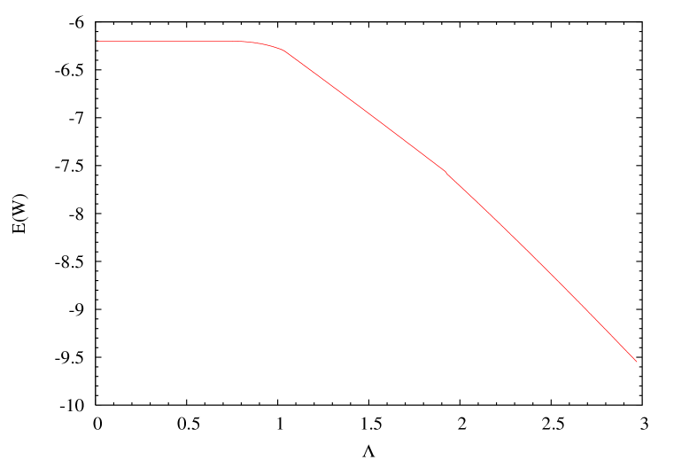
Figure 1: The vacuum energy $E(W)$ in the $SU(3)$ model as a function of $\Lambda=\Lambda_{1222}=\Lambda_{2212}$. Note the discontinuous slope near $\Lambda=1.9$.

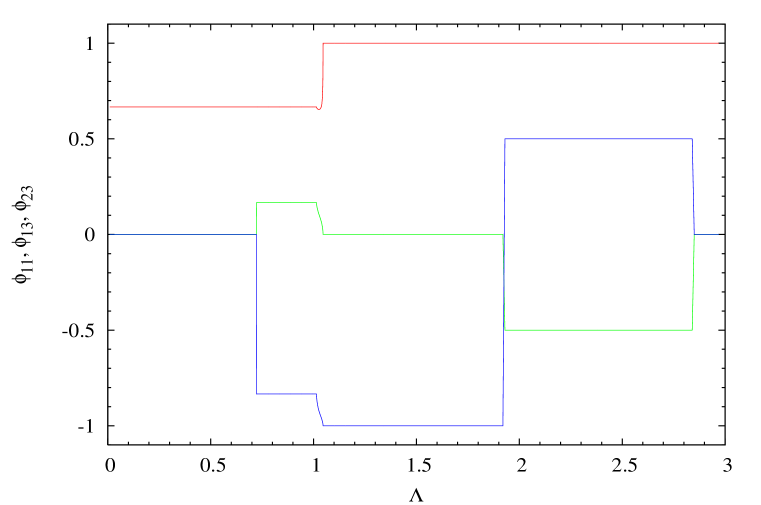
Figure 2: The $W$-phases $\phi_{11}/\pi$ (red), $\phi_{13}/\pi$ (green) and $\phi_{23}/\pi$ (blue) in the $SU(3)$ model. Phases $\phi_{13}$ and $\phi_{23}$ are undefined where $|W_{13}|$ and $|W_{23}|$ are zero.

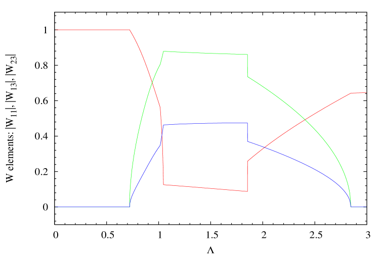
Figure 3: The $W$-magnitudes $|W_{11}|$ (red), $|W_{13}|$ (green) and $|W_{23}|$ (blue) in the $SU(3)$ model.

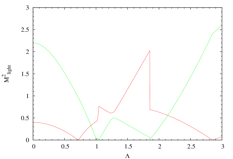
Figure 4: The $M^{2}$ of the lightest two pseudoGoldstone bosons in the $SU(3)$ model.

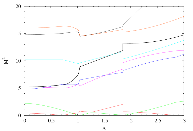
Figure 5: The $M^{2}$ of all eight pseudoGoldstone bosons in the $SU(3)$ model.

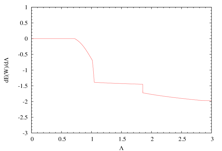
Figure 6: $dE(W)/d\Lambda$ in the $SU(3)$ model.

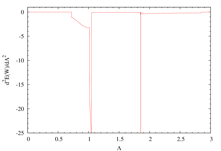
Figure 7: $d^{2}E(W)/d\Lambda^{2}$ in the $SU(3)$ model.

We classify the transitions between different CP phases as being of first order (1-OPT) or second order (2-OPT) depending on whether $dE(W)/d\Lambda$ or $d^{2}E(W)/d\Lambda^{2}$ is discontinuous at the transition. The second derivative is plotted in Fig. 7; we will discuss it in the next section. First-order transitions involve discontinuous changes in $W$-matrix elements. They occur only at CPC–PCP transitions. The elements of $W$ are continuous at second-order transitions. They occur at the boundaries between CPC or PCP regions and CPV ones, or at CPC–PCP boundaries such as $\Lambda=0.72$ and 2.85 where elements of $W$ continuously become nonzero or vanish.

We stress that the vanishing of an $M^{2}$ eigenvalue at a phase transition is not a consequence of increased chiral symmetry; the current corresponding to the massless boson is still not conserved at the transition. Rather, the boson’s masslessness is associated with a change in the discrete CP symmetry. We refer to the two chronically light PGBs of this model as accidental Goldstone bosons. They remain light because — in this model and others we have looked at — one is never very far from a phase transition. We explain in Sec. III why there are two AGBs in this model.

It is easy to understand why one PGB’s $M^{2}\rightarrow 0$ at a 2-OPT, $\Lambda=\Lambda_{*}$. As $\Lambda<\Lambda_{*}$ is increased, the true vacuum corresponding to one CP phase is becoming less stable, while the false vacuum corresponding to a different phase is becoming more stable. In this false vacuum, one PGB has $M^{2}<0$. In the true vacuum this PGB’s positive $M^{2}$ is decreasing while it is increasing in the false one. Since the 2-OPT is continuous, the two $M^{2}$ trajectories must cross at $M^{2}=0$. For a 1-OPT, there is a discontinuous jump in the lightest-$M^{2}$ as there is for all the others. Hence, there seems to be no argument for $M^{2}\rightarrow 0$. Nevertheless, in our calculations for this and other models, the lightest AGB mass appears to approach zero on one side of the 1-OPT as well. It is obvious that there are surfaces in the space of the $\Lambda_{ijkl}$ that separate the different CP phases and, at least for 2-OPT surfaces, an AGB mass vanishes there.

There is a clear level-crossing phenomenon in Fig. 4, in the CPC region near $\Lambda=1.25$. There we see the two lightest PGBs’ masses approach other and repel. The effect of this will be seen on the vevs of these states, discussed in Sec. V.

A comment on the units used for $M^{2}$ in Figs. 4 and 5 is in order: The quantity being plotted in these figures is actually $F_{\pi}^{2}M^{2}$. In our numerical calculations, we set $\Delta_{TT}=1$ so that $\Lambda_{ijkl}\Delta_{TT}={\cal O}(1)$. But, up to an anomalous dimension factor for the four-fermion condensate, $\Lambda_{ijkl}\Delta_{TT}\simeq\Lambda_{ijkl}\Lambda_{T}^{2}F_{\pi}^{4}$ where $\Lambda_{T}\simeq 4\pi F_{\pi}$. If, for example, $\Lambda_{ijkl}=(10\Lambda_{T})^{-2}$, then the vertical scale in Figs. 4,5 is in units of $10^{-2}F_{\pi}^{4}$. The AGB masses are then $M\mathrel{\hbox to0.0pt{\raise 2.20013pt\hbox{$<$}\hss}{\lower 2.20013pt\hbox{$\sim$}}}0.1F_{\pi}\simeq 10^{-2}\Lambda_{T}$.

Finally, we do not believe that these phase transitions and the associated vanishing of a PGB mass are mere artifacts of our using lowest-order chiral perturbation theory. Higher-order corrections may shift the surfaces in $\Lambda$-space separating the phases (not to mention expanding the dimensions of the space), and they may even eliminate existing transitions or add new ones. But we see no reason that phase linking, the transitions between various rational and irrational phase solutions, and the associated massless states would not occur for ${\cal H}^{\prime}$ with higher dimensional than four-fermion operators and vacuum energies involving higher powers of $W$ and $W^{\dagger}$.

III. Understanding the Phase Transitions I:
The Formula for $d^{2}E(W)/d\Lambda^{2}$

Considerable insight into the AGBs — their number and the connection between their vanishing masses and the behavior of the $W$-phases — can be gained from studying $d^{2}E(W)/d\Lambda^{2}$. For definiteness, we continue to consider a theory in which chiral flavor symmetry $G_{f}=SU(N)_{L}\otimes SU(N)_{R}$ is spontaneously broken in the vacuum $|\Omega\rangle$ to $S_{f}=SU(N)_{V}$. The chiral symmetry $G_{f}$ is also explicitly broken by an interaction ${\cal H}^{\prime}$ as in Eq. (2), for example. Suppose that ${\cal H}^{\prime}$ depends linearly on a parameter $\Lambda$. Write the vacuum energy of the properly aligned Hamiltonian as

$$E(W\equiv e^{2i{\boldsymbol{t}}\cdot{\boldsymbol{\omega}}})=\langle\Omega|{\cal H}^{\prime}({\boldsymbol{\omega}})|\Omega\rangle\equiv\langle\Omega|e^{i{\boldsymbol{Q}_{5}}\cdot{\boldsymbol{\omega}}}\,{\cal H}^{\prime}e^{-i{\boldsymbol{Q}_{5}}\cdot{\boldsymbol{\omega}}}|\Omega\rangle\,,$$ (13)

where $\omega_{a}$, $a=1,\dots,N^{2}-1$, is a $W$-phase at the minimum. Then (sum on repeated indices)

$$\frac{d^{2}E(W)}{d\Lambda^{2}}=-{\cal G}_{ac}(-{\boldsymbol{\omega}})\,(F_{\pi}^{2}M^{2})_{cd}\,{\cal G}_{db}({\boldsymbol{\omega}})\frac{d\omega_{a}}{d\Lambda}\frac{d\omega_{b}}{d\Lambda}\equiv-\frac{\partial^{2}E(W)}{\partial\omega_{a}\partial\omega_{b}}\,\frac{d\omega_{a}}{d\Lambda}\frac{d\omega_{b}}{d\Lambda}\,.$$ (14)

Equation (14) is derived in Appendix A. Here, $M^{2}$ is the PGB squared-mass matrix and ${\cal G}({\boldsymbol{\omega}})$ is the matrix

$${\cal G}_{ab}({\boldsymbol{\omega}})={\cal G}_{ba}(-{\boldsymbol{\omega}})=\left(\frac{e^{i{\boldsymbol{F}}\cdot{\boldsymbol{\omega}}}-1}{i{\boldsymbol{F}}\cdot{\boldsymbol{\omega}}}\right)_{ab}=\sum_{n=0}^{\infty}\frac{((i{\boldsymbol{F}}\cdot{\boldsymbol{\omega}})^{n})_{ab}}{(n+1)!}\,,$$ (15)

and $(F_{a})_{bc}=-if_{abc}$ is the adjoint representation of $G_{f}$. At a minimum, $\partial^{2}E(W)/\partial\omega_{a}\partial\omega_{b}$ is a positive-semidefinite matrix, so that $d^{2}E(W)/d\Lambda^{2}\leq 0$, as seen in Fig. 7.

To go further with Eq. (14), it is convenient to replace $W$ by its diagonalized form:

$$W=e^{2i{\boldsymbol{t}}\cdot{\boldsymbol{\omega}}}=UW_{D}U^{\dagger}\equiv U\left(e^{2i{\boldsymbol{t}_{D}}\cdot{\boldsymbol{\omega}_{D}}}\right)U^{\dagger}\,.$$ (16)

Here, $U$ is the $SU(N)$ matrix which diagonalizes $W$ to $W_{D}$ and ${\boldsymbol{t}}\cdot{\boldsymbol{\omega}}$ to ${\boldsymbol{t}_{D}}\cdot{\boldsymbol{\omega}_{D}}$. There are $N-1$ diagonal phases $\omega_{Da}$, $a=n^{2}-1$ with $n=2,\dots,N$. They depend in complicated ways on the $N^{2}-1$ phases $\omega_{a}$ and the parameters in $U$. For $t_{a}\in{\boldsymbol{N}}$, define the real orthogonal matrix $S$ by $S_{ab}=2{\rm Tr}(U^{\dagger}t_{a}Ut_{b})$. Then, $\sum_{a=3}^{N^{2}-1}t_{Da}\omega_{Da}\equiv U^{\dagger}(\sum_{b}t_{b}\omega_{b})U=\sum_{b,c}S_{bc}t_{c}\omega_{b}$ implies

$$\sum_{b}S_{ba}\omega_{b}=\left\{\begin{array}[]{l}\omega_{Da}\,\,\,{\rm for}\,\,a=3,8,\dots,N^{2}-1\\ 0\,\,\,{\rm otherwise.}\\ \end{array}\right.$$ (17)

Next, define $M^{2}_{U}$ by

$$(F_{\pi}^{2}M^{2})_{cd}=S_{ce}\left(F_{\pi}^{2}M^{2}_{U}\right)_{ef}S^{-1}_{fd}\,.$$ (18)

For ${\cal H}^{\prime}$ of the form in Eq. (2), $M^{2}_{U}$ is given by

$$\left(F_{\pi}^{2}M^{2}_{U}\right)_{ef} = 2\sum_{ijkl}\Lambda^{U}_{ijkl}\Biggl{[}\left(\left\{t_{e},t_{f}\right\}W_{D}^{\dagger}\right)_{li}\thinspace W_{Djk}+\left(W_{D}\left\{t_{e},t_{f}\right\}\right)_{jk}\thinspace W_{Dli}^{\dagger}$$ (19)

$$\qquad-2\left(t_{e}W_{D}^{\dagger}\right)_{li}\thinspace\left(W_{D}t_{f}\right)_{jk}-2\left(t_{f}W_{D}^{\dagger}\right)_{li}\thinspace\left(W_{D}t_{e}\right)_{jk}\thinspace\Biggr{]}\Delta_{TT}\,;$$

$$\Lambda^{U}_{ijkl} = \sum_{i^{\prime}j^{\prime}k^{\prime}l^{\prime}}\Lambda_{i^{\prime}j^{\prime}k^{\prime}l^{\prime}}U^{\dagger}_{ii^{\prime}}U_{j^{\prime}j}U^{\dagger}_{kk^{\prime}}U_{l^{\prime}l}\,.$$ (20)

The relation $f_{def}S_{da}S_{eb}S_{fc}=f_{abc}$ and Eq. (17) imply $S^{-1}{\boldsymbol{F}}\cdot{\boldsymbol{\omega}}S={\boldsymbol{F}_{D}}\cdot{\boldsymbol{\omega}_{D}}$, where $F_{Da}$ is a diagonal generator in the adjoint representation. Thus, Eq. (14) can be cast in the form

$$\frac{d^{2}E(W)}{d\Lambda^{2}}=-\left({\cal G}(-{\boldsymbol{\omega}_{D}})\,F_{\pi}^{2}M^{2}_{U}\,{\cal G}({\boldsymbol{\omega}_{D}})\right)_{ab}\left[\frac{d\omega_{Da}}{d\Lambda}-\omega_{c}\frac{dS^{-1}_{ac}}{d\Lambda}\right]\left[\frac{d\omega_{Db}}{d\Lambda}-\omega_{d}\frac{dS^{-1}_{bd}}{d\Lambda}\right]\,.$$ (21)

This is our key equation.

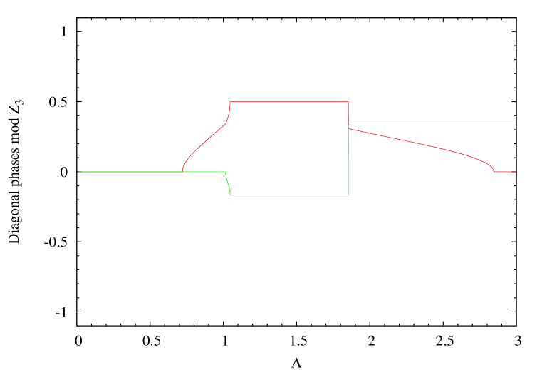
Figure 8: The normalized diagonal phases $\widehat{\omega}_{D3}/\pi$ (red) and $\widehat{\omega}_{D8}/\pi$ (green) in the $SU(3)$ model.

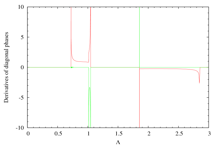
Figure 9: $d(\widehat{\omega}_{D3}/\pi)/d\Lambda$ (red) and $d(\widehat{\omega}_{D8}/\pi)/d\Lambda$ (green) in the $SU(3)$ model.

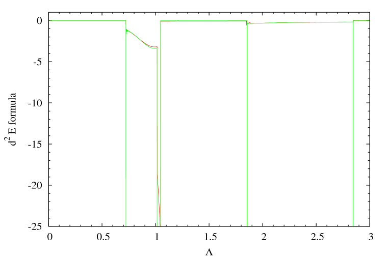
Figure 10: A comparison of $d^{2}E(W)/d\Lambda^{2}$ (red) and the right-hand side of Eq. (22) (green) in the $SU(3)$ model.

In Sec. II we saw that all $W$-phases $\phi_{ij}$ are rational multiples of $\pi$ in the CPC and PCP phases. In Fig. 8 we plot the normalized diagonal phases $\widehat{\omega}_{Da}=\omega_{Da}/\sqrt{n(n-1)/2}$ for the $SU(3)$ model ($n=2,3$). We see that in CPC phases, both $\widehat{\omega}_{Da}$ are rational multiples of $\pi$; in PCP phases, only $\widehat{\omega}_{D8}$ is rational; in the CPV phase, both are irrational. This will be explained in Sec. IV. It is remarkable that, even though $\widehat{\omega}_{D3}$ is irrational in the PCP phases, all $\phi_{ij}$ are rational there.

One sees in Fig. 8 that the slope of one or both of the $\widehat{\omega}_{Da}$ is singular at every 2-OPT ($d\widehat{\omega}_{D3}/d\Lambda$ is merely discontinuous at $\Lambda=1.0140$) while both $\widehat{\omega}_{Da}$ are discontinuous at the 1-OPT at $\Lambda=1.85$. Looking back at Fig. 2, this behavior is clearly reflected in all the $\phi_{ij}$; it is especially dramatic at the 2-OPTs near $\Lambda=1$. The slopes $d\widehat{\omega}_{Da}/d\Lambda$ are plotted in Fig. 9. Away from the phase transitions, they are not large except in the narrow CPV phase where the $\widehat{\omega}_{Da}$ are rapidly varying. The singular behavior of the $\widehat{\omega}_{Da}$ in Fig. 8 is just what we expect of order parameters at first and second-order phase transitions. Therefore, we interpret the diagonal phases $\omega_{Da}$ as the order parameters for the phase transitions we’ve been observing. Here, however, the transitions are between different phases of a discrete symmetry.

In general, the $dS^{-1}_{ac}/d\Lambda$ in Eq. (21) are small. Thus, $d^{2}E(W)/d\Lambda^{2}$ is well approximated by keeping only the $(d\omega_{Da}/d\Lambda)\,(d\omega_{Db}/d\Lambda)$ terms in Eq. (21). Just how good this approximation is can be seen by looking at the region $\Lambda=1.05$ to 1.85 in Fig. 7. There $d\omega_{Da}/d\Lambda\equiv 0$, while $d^{2}E(W)/d\Lambda^{2}$ is negative, but very small. If we drop the $dS^{-1}_{ac}/d\Lambda$ terms, Eq. (21) simplifies greatly because $(F_{Dc})_{ab}=0$ and ${\cal G}_{ab}({\boldsymbol{\omega}_{D}})=\delta_{ab}$ when index $a$ or $b=3,8,\dots,N^{2}-1$. Then

$$\frac{d^{2}E(W)}{d\Lambda^{2}}\cong-\left(F_{\pi}^{2}M^{2}_{U}\right)_{ab}\frac{d\omega_{Da}}{d\Lambda}\,\frac{d\omega_{Db}}{d\Lambda}\,.$$ (22)

In Fig. 10 we compare $d^{2}E(W)/d\Lambda^{2}$ with the right-hand side of Eq. (22). The agreement is excellent except in the narrow CPV region with rapidly varying phases. There, the discrepancy is due both to the neglect of the $\omega_{c}dS^{-1}_{ac}/d\Lambda$-terms and the difficulty of computing the derivatives as they become divergent.

Equation (22) makes a clear connection between the lightest PGBs, the ones we call AGBs, and the diagonal phases $\omega_{Da}$. We believe the association is one-to-one, and that is why the $SU(3)$ model has two AGBs. At 2-OPTs, the $\omega_{Da}$ are continuous, but at least some $d\omega_{Da}/d\Lambda$ are divergent. Meanwhile, $d^{2}E(W)/d\Lambda^{2}$ is finite, though discontinuous. This is possible only if a zero eigenvalue of the PGB $M^{2}$-matrix appears exactly at the transition to cancel singularities in the $d\omega_{Da}/d\Lambda$. This is another reason we believe that the vanishing of AGB masses at phase transitions is not an artifact of lowest-order chiral perturbation theory. At a 1-OPT at $\Lambda_{*}$, $\omega_{Da}$ is discontinuous and $d\omega_{Da}/d\Lambda\propto\delta(\Lambda-\Lambda_{*})$. On the other hand, all the PGB masses are discontinuous there, so we expect $d^{2}E(W)/d\Lambda^{2}\propto\delta(\Lambda-\Lambda_{*})$, i.e., a discontinuous slope in $E(W)$, as well.

IV. Understanding the Phase Transitions II:
The Character of $\widehat{W}=D_{R}D_{L}K$

In Sec. II we showed that, in a basis in which the aligning matrix is $\widehat{W}=D_{R}WD_{R}^{\dagger}=D_{R}D_{L}K$, the LR terms in ${\cal H}^{\prime}(\widehat{W})$ are real in the PCP and CPC phases. The matrix $\widehat{W}$ has the same eigenvalues as $W$, therefore the same diagonal phases $\widehat{\omega}_{Da}$. However, it is easier to analyze the possibilities for the $\widehat{\omega}_{Da}$ by considering $\widehat{W}$.

Consider first the CPC phase. In that case, $\widehat{W}=e^{2im\pi/N}\widetilde{W}$ where $\widetilde{W}$ is an $SO(N)$ matrix and $m=0,\dots,N-1$. Denote $\widetilde{W}$’s eigenvalues by $e^{i\eta_{i}}$, $i=1,\dots,N$ where the eigenphases satisfy $\sum_{i}\eta_{i}=0$ (mod $2\pi$). If $N$ is even, the eigenphases form conjugate pairs, $(e^{i\eta_{i}},e^{-i\eta_{i}})$ for $i=1,\dots,N/2$. If $N$ is odd, one eigenvalue, say $e^{i\eta_{N}}$, is $+1$. The ordering of the $\eta_{i}$ is arbitrary. Given an ordering, we can calculate the diagonal phases from

$$\widehat{\omega}_{D,N^{2}-1} = -\left(\frac{1}{N-1}\right)(2m\pi/N+\eta_{N})\,,$$

$$\widehat{\omega}_{D,(N-1)^{2}-1} = -\left(\frac{1}{N-2}\right)((2m\pi+\eta_{N})/(N-1)+\eta_{N-1})\,,\dots$$ (23)

Because of the $Z_{N}$ ambiguity in $\widetilde{W}$, we can set $m=0$ if we wish.

Now, if $\widetilde{W}$ is also symmetric, then all its eigenvalues are real, therefore equal $\pm 1$, with an even number of $-1$’s. All its eigenphases of $\widehat{W}$ would be rational multiples of $\pi$ and, then, so would their linear combinations forming the $\widehat{\omega}_{Da}$. In the models we studied numerically, $\widetilde{W}$ is symmetric to about a part in $10^{3}$ in all nontrivial CPC phases, i.e., when $\widetilde{W}$ is not merely proportional to the identity. Hence, the $\widehat{\omega}_{Da}$ are rational to about the same accuracy in these calculations. The difference from exactly rational phases is not visible in the CPC regions of Fig. 8. This closeness to rational phases is tantalizing, but we believe it is an unintended artifact of the way we chose the couplings $\Lambda_{ijkl}$ in the $SU(3)$ model. Those couplings seem to favor minimizing $E$ with a symmetric $\widetilde{W}$; we have modified them to make $\widetilde{W}$ non-symmetric in a CPC phase.

Turning to the PCP case, in which the phases $\phi_{ij}$ of $W_{ij}$ are different rational multiples of $\pi$, we have identified two subphases: PCP-1 in which $\widehat{W}=e^{i\phi}\widetilde{W}$ with $\widetilde{W}$ a real $O(N)$ matrix, and PCP-2 in which $\widehat{W}$ cannot be written in this way. In PCP-1, which is what we observed in our $SU(3)$ model, $\phi=2m\pi/N$ if $\det\widetilde{W}=1$, while $\phi=(2m+1)\pi/N$ if $\det\widetilde{W}=-1$. If $N$ is odd and $\det\widetilde{W}=-1$, we can change the sign of $\widetilde{W}$ and take $\phi=2m\pi/N$. For odd $N$, then, the eigenvalues of $\widetilde{W}$ form $(N-1)/2$ pairs, $(e^{i\eta_{i}},e^{-i\eta_{i}})$ plus one real eigenvalue, $e^{i\eta_{N}}=1$ and, so, $\widetilde{W}$ has $2n+1$ truly rational eigenphases, $n=0,1,\dots,(N-1)/2$. As in Eq. (IV. Understanding the Phase Transitions II: The Character of $\widehat{W}=D_{R}D_{L}K$), we can define $\widehat{\omega}_{D,N^{2}-1}=-2m\pi/N(N-1)$. If $N$ is even and $\det\widetilde{W}=1$, $\widetilde{W}$ has $2n=0,2,\dots,N$ rational phases. In this case, there may be no rational $\widehat{\omega}_{Da}$ even though all $W$-phases $\phi_{ij}$ are rational. If $\det\widetilde{W}=-1$, there must be a real pair of eigenphases, $(1,-1)$, so there are will be at least two rational $\widehat{\omega}_{Da}$. We can choose them to be $\widehat{\omega}_{D,N^{2}-1}=-((2m+1)\pi/N\pm\pi)/(N-1)$ and $\widehat{\omega}_{D,(N-1)^{2}-1}=-((2m+1)\pi\pm\pi)/(N-1)(N-2)$.

Finally, in a PCP-2 phase, there is no argument that any of the $\widehat{\omega}_{Da}$ are rational. The same is of course true in a CPV phase, and we find only irrational phases in both.

V. VEVs of the AGBs

In this section we investigate whether AGBs can serve as light composite Higgs bosons. We have seen that they are usually much lighter than the scale $\Lambda_{T}\simeq 4\pi F_{\pi}$ of their strong binding interaction. Having associated the AGBs with the diagonal phases $\omega_{Da}$ and, in turn, identified these as the order parameters of the various CP phases, it is natural to connect the vacuum expectation values of the AGBs with these phases. The question studied here is whether these vevs can also be much less than $\Lambda_{T}$.

In a nonlinear sigma-model formulation of the $G_{f}=SU(N)_{L}\otimes SU(N)_{R}$ model, we would replace $\bar{T}_{Rj}T_{Li}$ by $F_{\pi}^{3}\Sigma_{ij}$, where $\Sigma=\exp{(2i{\boldsymbol{t}}\cdot{\boldsymbol{\pi}}/F_{\pi})}$. Under a $G_{f}$ transformation, $\Sigma\rightarrow W_{L}\Sigma W_{R}^{\dagger}$. Minimizing the energy $E(W)$ in this formulation amounts to determining the vacuum expectation values $\langle\pi_{a}\rangle=\langle\Omega|\pi_{a}|\Omega\rangle$ in the tree approximation. Thus, these vevs are related to the minimizing-$W$ phases $\omega_{a}$ by

$$\langle\pi_{a}\rangle=\omega_{a}F_{\pi}\,.$$ (24)

To determine the vevs of the $N-1$ AGBs of the model, we write

$$M^{2}_{ab}\,\omega_{a}\omega_{b} = M^{2}_{ab}S_{ac}S_{bd}\,\omega_{Dc}\omega_{Dd}$$ (25)

$$= (M_{U}^{2})_{ab}\,\omega_{Da}\omega_{Db}=(VM_{D}^{2}V^{-1})_{ab}\,\omega_{Da}\omega_{Db}\,,$$

where $V$ is the $SO(N)$ matrix which diagonalizes $M_{U}^{2}=S^{-1}M^{2}S$ to $M_{D}^{2}$. The mass eigenstate vevs $v_{a}$, in particular, those of the AGBs, are then

$$v_{a}=V_{ba}\,\omega_{Db}F_{\pi}=(V^{-1}S^{-1})_{ab}\,\omega_{b}F_{\pi}\,.$$ (26)

This definition of the AGB vevs is independent of the convention used to define the $\omega_{Da}$. Note that, so long as vacuum alignment preserves electric charge conservation, $W_{ij}=\delta_{ij}$ in electrically charged sectors and all AGBs are electrically neutral.

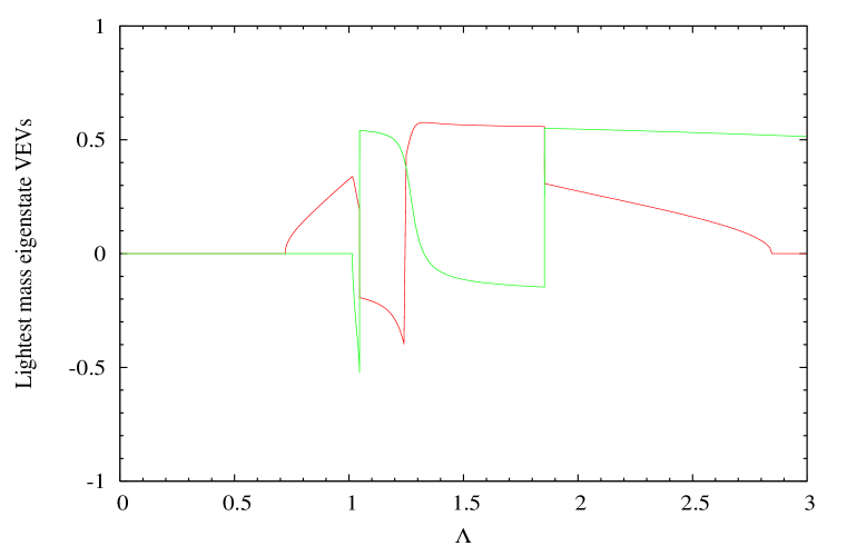
Figure 11: The vevs $(v_{a}/F_{\pi})/\pi$ of the lightest two pseudoGoldstone bosons in the $SU(3)$ model. The colors match those in Fig. 4.

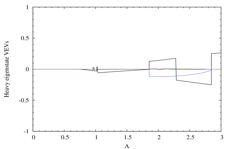
Figure 12: The vevs $(v_{a}/F_{\pi})/\pi$ of the six heavier pseudoGoldstone bosons in the $SU(3)$ model. The colors match those in Fig. 5.

An AGB may be a suitable light composite Higgs if $|v_{a}/F_{\pi}|\ll 4\pi$. These vevs are plotted in Fig. 11 for the two lightest AGBs of the $SU(3)$ model. They are indeed generally small, with $|v_{a}|\mathrel{\hbox to0.0pt{\raise 2.20013pt\hbox{$<$}\hss}{\lower 2.20013pt\hbox{$\sim$}}}0.03$–$0.1\Lambda_{T}$ in all CP phases. Similar results are obtained in an $SU(4)$-model calculation. The AGBs’ vevs tend to track $\omega_{D3}$ and $\omega_{D8}$, except near $\Lambda=1.25$. These small vevs seem to be due to the $1/N$ factors in Eq. (IV. Understanding the Phase Transitions II: The Character of $\widehat{W}=D_{R}D_{L}K$) and to the fact that $|V_{ab}|<1$. Changes in the vevs due to higher-corrections to ${\cal H}^{\prime}$ should be small unless those corrections induce a first-order phase transition. The rapid variation in the vevs near $\Lambda=1.25$ is due to the level-crossing visible there in Fig. 4. We have seen the same phenomenon analytically in the isospin-violating version of the $SU(3)$ model described in Appendix B. Finally, if the $G_{f}$ symmetries were gauged with coupling $g$, the AGBs would give masses $\sim gv_{a}$ to the gauge bosons that are very much less than the underlying dynamical scale $\Lambda_{T}$.

The mass eigenstate vevs of the heavier PGBs are shown in Fig. 12. They are generally very small, or at most comparable to those of the light AGBs. This confirms that the light AGBs correspond to the diagonal phases $\omega_{Da}$. Further, if the heavier PGBs are coupled to gauge bosons, they generally contribute negligibly to their mass, and never more than the AGBs do. From an experimental point of view, one would probably conclude that the gauge symmetries are broken by light composite Higgs bosons at a scale well below $\Lambda_{T}$. Small vevs for the heavier PGBs raise the interesting possibility that a heavy composite Higgs can naturally give small masses to gauge bosons, with no contribution coming from the light AGBs. Experimentally, the only sign of the gauge symmetry’s breaking at energies of order $v_{a}$ would be a (temporary) breakdown of perturbative unitarity!

VI. Summary and Future Work

In this paper we studied vacuum alignment in theories in which the global chiral symmetry $G_{f}$ of a set of $N$ massless Dirac fermions is broken both spontaneously by their strong interactions and explicitly by terms in a weak perturbation ${\cal H}^{\prime}$. This perturbation is chosen to give mass to all the Goldstone bosons of the spontaneous symmetry breaking. We showed that, as a coupling parameter $\Lambda$ in ${\cal H}^{\prime}$ is changed, the system moves through various phases of the discrete symmetry, CP. We identified three main phases: CP-conserving, in which the aligning matrix $W\in SU(N)$ is real up to a $Z_{N}$ factor and the aligned Hamiltonian ${\cal H}^{\prime}(W)$ is real; CP-violating, in which $W$ and ${\cal H}^{\prime}(W)$ are essentially complex; and a new phase, pseudoCP-conserving, in which the phases in $W$ are different rational multiples of $\pi$ and so are the phases of ${\cal H}^{\prime}(W)$. For the class of models we studied, it was actually possible in the PCP phase to make a transformation that rendered the explicit $G_{f}$-breaking terms in ${\cal H}^{\prime}(W)$ real.

Most important, we found that the transitions between different CP phases are of classic first or second-order, defined as whether the first or second derivative of the vacuum energy $E(W)=\langle\Omega|{\cal H}^{\prime}(W)|\Omega\rangle$ with respect to $\Lambda$ is discontinuous at the transition. At all these transitions a pseudoGoldstone boson’s mass vanishes. Following Dashen [1], we call these accidental Goldstone bosons, AGBs, but we argued that their presence is not a mere consequence of the lowest-order chiral perturbation theory we employ to calculate their masses. Rather, they are a necessary consequence of the CP-phase transitions, phenomena we believe transcend our ${\cal O}({\cal H}^{\prime})$ approximation. The relative frequency of CP-phase transitions makes AGBs common: there generally seem to be several such states, much lighter than the other PGBs. We derived a remarkable formula for $d^{2}E(W)/d\Lambda^{2}$ that establishes a one-to-one correspondence between the AGBs and the eigenphases $\omega_{Da}$ of the diagonalized form $W_{D}$ of $W$. In the $SU(N)$ models we studied, $W_{D}=\exp{(2i\sum_{a=3}^{N^{2}-1}t_{Da}\,\omega_{Da})}$ and there are $N-1$ AGBs. The vanishing of an AGB mass at some $\Lambda=\Lambda_{*}$ is directly correlated with the singular behavior of its corresponding combination of $\omega_{Da}$.

The AGB masses are naturally much less than the scale $\Lambda_{T}\simeq 4\pi F_{\pi}$ of their strong binding interaction. Equally interesting, we found that their vacuum expectation values also are often much less than $\Lambda_{T}$. Thus, they are prototypes for light composite Higgs bosons for electroweak symmetry breaking. To make a realistic model, we have to find a way to embed $SU(2)\otimes U(1)$ into the AGBs’ symmetry group $G_{f}$ without their constituent $T$-fermions’ condensates breaking electroweak symmetry at $\Lambda_{T}$. One way that does not work is a technicolor-like scheme with $N$ doublets, $T_{L,R\,i}=(U,D)_{L,R\,i}$, and a chiral $SU(2N)_{L}\otimes SU(2N)_{R}$ symmetry breaking down to $SU(2N)$. These fermions must transform vectorially under $SU(2)\otimes U(1)$, with weak hypercharges $Y_{i}$. The $Y_{i}$ must be chosen so that the PGB-mass generating ${\cal H}^{\prime}$ is $SU(2)\otimes U(1)$-invariant. Then it is impossible for $\Sigma=e^{2i{\boldsymbol{t}}\cdot{\boldsymbol{\pi}}}$ to develop a vacuum expectation value which both conserves electric charge, $Q=T_{3}+Y$, and breaks electroweak symmetry in the correct way; in particular, the $U(1)$ remains unbroken. Another difficult problem is coupling the AGBs to quarks and leptons so that their vevs can give them mass. Compounding that difficulty is the need to avoid unwanted flavor-changing neutral current interactions. Presumably, one must be in a PCP phase so that weak, but not strong, CP violation is transmitted to the quarks through the Yukawa couplings to the $\Sigma$-field [4].

Appendix A: Derivation of the Formula for $d^{2}E(W)/d\Lambda^{2}$

Consider a theory in which the chiral flavor symmetry $G_{f}$ is spontaneously broken in the vacuum $|\Omega\rangle$ to $S_{f}$. The chiral symmetry $G_{f}$ is also explicitly broken by an interaction ${\cal H}^{\prime}$. Suppose that ${\cal H}^{\prime}$ depends linearly on a parameter $\Lambda$. Write the minimized vacuum energy as

$$E(W_{0}\equiv e^{i{\boldsymbol{t}}\cdot{\boldsymbol{\omega}_{0}}})=\langle\Omega|{\cal H}^{\prime}({\boldsymbol{\omega}_{0}})|\Omega\rangle\equiv\langle\Omega|e^{i{\boldsymbol{Q}}\cdot{\boldsymbol{\omega}_{0}}}\,{\cal H}^{\prime}\,e^{-i{\boldsymbol{Q}}\cdot{\boldsymbol{\omega}_{0}}}|\Omega\rangle\,.$$ (27)

Here, $Q_{a}$ is a generator of $G_{f}$ and $t_{a}$ is its matrix representation. Charges $Q_{a}\in S_{f}$ annihilate $|\Omega\rangle$; charges in $G_{f}/S_{f}$ create a Goldstone boson $\pi_{a}$ from the vacuum with strength $F_{\pi}$. We have reintroduced the subscript “0” to emphasize that $W_{0}$ is the unitary aligning matrix which minimizes the vacuum energy.

Let us study how the minimized energy changes as we vary $\Lambda$. The first derivative is (sum on repeated indices)

$$\frac{dE(W_{0})}{d\Lambda}=\langle\Omega|e^{i{\boldsymbol{Q}}\cdot{\boldsymbol{\omega}_{0}}}\,\frac{\partial{\cal H}^{\prime}}{\partial\Lambda}\,e^{-i{\boldsymbol{Q}}\cdot{\boldsymbol{\omega}_{0}}}|\Omega\rangle+\left[\frac{\partial}{\partial\omega_{a}}\langle\Omega|{\cal H}^{\prime}({\boldsymbol{\omega}})|\Omega\rangle\right]_{{\boldsymbol{\omega}}={\boldsymbol{\omega}_{0}}}\frac{d\omega_{a,0}}{d\Lambda}\,.$$ (28)

The second term vanishes because $E(W)$ is stationary at extrema. Differentiating again, and using our linearity assumption, $\partial^{2}{\cal H}^{\prime}/\partial\Lambda^{2}=0$, we get

$$\frac{d^{2}E(W_{0})}{d\Lambda^{2}} = \left[\frac{\partial}{\partial\omega_{a}}\langle\Omega|e^{i{\boldsymbol{Q}}\cdot{\boldsymbol{\omega}}}\,\frac{\partial{\cal H}^{\prime}}{\partial\Lambda}\,e^{-i{\boldsymbol{Q}}\cdot{\boldsymbol{\omega}}}|\Omega\rangle\right]_{{\boldsymbol{\omega}}={\boldsymbol{\omega}_{0}}}\frac{d\omega_{a,0}}{d\Lambda}$$ (29)

$$= i{\cal G}_{ba}({\boldsymbol{\omega}_{0}})\,\langle\Omega|\bigl{[}Q_{b},\,e^{i{\boldsymbol{Q}}\cdot{\boldsymbol{\omega}_{0}}}\,\frac{\partial{\cal H}^{\prime}}{\partial\Lambda}\,e^{-i{\boldsymbol{Q}}\cdot{\boldsymbol{\omega}_{0}}}\bigr{]}|\Omega\rangle\,\frac{d\omega_{a,0}}{d\Lambda}\,,$$

where

$${\cal G}_{ab}({\boldsymbol{\omega}})={\cal G}_{ba}(-{\boldsymbol{\omega}})=\left(\frac{e^{i{\boldsymbol{F}}\cdot{\boldsymbol{\omega}}}-1}{i{\boldsymbol{F}}\cdot{\boldsymbol{\omega}}}\right)_{ab}=\sum_{n=0}^{\infty}\frac{((i{\boldsymbol{F}}\cdot{\boldsymbol{\omega}})^{n})_{ab}}{(n+1)!}\,,$$ (30)

and $(F_{a})_{bc}=-if_{abc}$ is the adjoint representation of $Q_{a}$. The proof of the second equality in Eq. (29) will be given below. Now,

$$\langle\Omega|\bigl{[}Q_{b},\,e^{i{\boldsymbol{Q}}\cdot{\boldsymbol{\omega}_{0}}}\,\frac{\partial{\cal H}^{\prime}}{\partial\Lambda}\,e^{-i{\boldsymbol{Q}}\cdot{\boldsymbol{\omega}_{0}}}\bigr{]}|\Omega\rangle = \frac{d}{d\Lambda}\langle\Omega|\bigl{[}Q_{b},\,e^{i{\boldsymbol{Q}}\cdot{\boldsymbol{\omega}_{0}}}\,{\cal H}^{\prime}\,e^{-i{\boldsymbol{Q}}\cdot{\boldsymbol{\omega}_{0}}}\bigr{]}|\Omega\rangle$$

$$\,\,-\frac{\partial}{\partial\omega_{c,0}}\langle\Omega|\bigl{[}Q_{b},\,e^{i{\boldsymbol{Q}}\cdot{\boldsymbol{\omega}_{0}}}\,{\cal H}^{\prime}\,e^{-i{\boldsymbol{Q}}\cdot{\boldsymbol{\omega}_{0}}}\bigr{]}|\Omega\rangle\,\frac{d\omega_{c,0}}{d\Lambda}\,.$$

The first term on the right vanishes by the extremal condition on $E(W)$ (see Eq. (Appendix A: Derivation of the Formula for $d^{2}E(W)/d\Lambda^{2}$) below). The second term may be rewritten using Eqs. (29) and (7):

$$\frac{\partial}{\partial\omega_{c,0}}\langle\Omega|\bigl{[}Q_{b},\,e^{i{\boldsymbol{Q}}\cdot{\boldsymbol{\omega}_{0}}}\,{\cal H}^{\prime}\,e^{-i{\boldsymbol{Q}}\cdot{\boldsymbol{\omega}_{0}}}\bigr{]}|\Omega\rangle = i{\cal G}_{dc}({\boldsymbol{\omega}_{0}})\langle\Omega|\bigl{[}Q_{b},\bigl{[}Q_{d},\,{\cal H}^{\prime}({\boldsymbol{\omega}_{0}})\bigr{]}\bigr{]}|\Omega\rangle$$ (32)

$$\equiv -i\left(F_{\pi}^{2}M^{2}{\cal G}({\boldsymbol{\omega}_{0}})\right)_{bc}\,.$$

This gives the desired result:

$$\frac{d^{2}E(W_{0})}{d\Lambda^{2}}=-\left({\cal G}(-{\boldsymbol{\omega}_{0}})\,F_{\pi}^{2}M^{2}\,{\cal G}({\boldsymbol{\omega}_{0}})\right)_{ab}\frac{d\omega_{a,0}}{d\Lambda}\frac{d\omega_{b,0}}{d\Lambda}\,.$$ (33)

The proof of the second equality in Eq. (29) follows from the identities

$$e^{-i{\boldsymbol{Q}}\cdot{\boldsymbol{\omega}}}Q_{a}e^{i{\boldsymbol{Q}}\cdot{\boldsymbol{\omega}}} = \left(e^{i{\boldsymbol{F}}\cdot{\boldsymbol{\omega}}}\right)_{ab}Q_{b}\,;$$ (34)

$$e^{-i{\boldsymbol{Q}}\cdot{\boldsymbol{\omega}}}\frac{\partial}{\partial\omega_{a}}e^{i{\boldsymbol{Q}}\cdot{\boldsymbol{\omega}}} = i{\cal G}_{ab}({\boldsymbol{\omega}})Q_{b}\,.$$ (35)

These imply

$$\frac{\partial}{\partial\omega_{a}}e^{i{\boldsymbol{Q}}\cdot{\boldsymbol{\omega}}}=i{\cal G}_{ba}({\boldsymbol{\omega}})Q_{b}e^{i{\boldsymbol{Q}}\cdot{\boldsymbol{\omega}}}\,.$$ (36)

Hence,

$$\frac{\partial}{\partial\omega_{a}}{\cal H}^{\prime}({\boldsymbol{\omega}})\equiv\frac{\partial}{\partial\omega_{a}}\left(e^{i{\boldsymbol{Q}}\cdot{\boldsymbol{\omega}}}\,{\cal H}^{\prime}\,e^{-i{\boldsymbol{Q}}\cdot{\boldsymbol{\omega}}}\right)=i{\cal G}_{ba}({\boldsymbol{\omega}})\bigl{[}Q_{b},{\cal H}^{\prime}({\boldsymbol{\omega}})\bigr{]}$$

$$\Longrightarrow \frac{\partial E(W)}{\partial\omega_{a}}\biggr{|}_{{\boldsymbol{\omega}}={\boldsymbol{\omega}_{0}}}\equiv i{\cal G}_{ba}({\boldsymbol{\omega}_{0}})\langle\Omega|\bigl{[}Q_{b},{\cal H}^{\prime}({\boldsymbol{\omega}_{0}})\bigr{]}|\Omega\rangle=0\,.$$

Since ${\cal G}({\boldsymbol{\omega}})$ is invertible, this implies $\langle\Omega|[Q_{a},{\cal H}^{\prime}({\boldsymbol{\omega}_{0}})]|\Omega\rangle=0$. Differentiating again and using Eq. (7) gives the second half of Eq. (14):

$$\frac{\partial^{2}E(W_{0})}{\partial\omega_{a,0}\partial\omega_{b,0}}=\left({\cal G}(-{\boldsymbol{\omega}_{0}})\,F_{\pi}^{2}M^{2}\,{\cal G}({\boldsymbol{\omega}_{0}})\right)_{ab}\,.$$ (38)

In deriving our formula, we ignored the singularities in $d\omega_{a,0}/d\Lambda$ at phase transitions. This is not a problem at a 2-OPT where the zero in $M^{2}$ cancels the divergence in the derivatives. At a 1-OPT, $d\omega_{a,0}/d\Lambda$ and $d^{2}E(W_{0})/d\Lambda^{2}$ are proportional to $\delta$-functions, so the formula, while consistent, really has no meaning there.

Appendix B: The CP Phase Transition in
Dashen’s Three-Quark Model

We illustrate Eq. (14) with the model Dashen discussed in Ref. [1]. Consider QCD with three massless quarks, $u,d,s$. Their chiral flavor symmetry $G_{f}=SU(3)_{L}\otimes SU(3)_{R}$ is spontaneously broken to $S_{f}=SU(3)_{V}$ in the vacuum $|\Omega\rangle$ defined by

$$\langle\Omega|\bar{q}_{Rj}q_{Li}|\Omega\rangle=\langle\Omega|\bar{q}_{Li}q_{Rj}|\Omega\rangle=-\delta_{ij}\Delta_{q}\,,$$ (39)

where $\Delta_{q}\simeq 2\pi F_{\pi}^{3}$. The $G_{f}$-symmetry is also explicitly broken by

$${\cal H}^{\prime}=\bar{q}_{R}M_{q}q_{L}+\bar{q}_{L}M_{q}^{\dagger}q_{R}\equiv\bar{q}M_{q}q\thinspace,$$ (40)

where the (assumed) real quark mass matrix is

$$M_{q}=M_{q}^{\dagger}\equiv\pm\left(\begin{array}[]{ccc}m_{u}&0&0\\ 0&m_{d}&0\\ 0&0&m_{s}\\ \end{array}\right)=\pm m_{s}\left(\begin{array}[]{ccc}\Lambda&0&0\\ 0&\Lambda&0\\ 0&0&1\\ \end{array}\right)$$ (41)

For simplicity, we assume isospin invariance, $m_{u}=m_{d}=m_{s}\Lambda$, with $\Lambda\geq 0$. This Hamiltonian conserves CP.

The vacuum energy to be minimized is

$$E(W=W_{L}W_{R}^{\dagger}) = \langle\Omega|\bar{q}_{R}(W_{R}^{\dagger}M_{q}W_{L})q_{L}+\bar{q}_{L}(W_{L}^{\dagger}M_{q}W_{R})q_{R}|\Omega\rangle$$ (42)

$$= -{\rm Tr}\left(M_{q}W+M_{q}^{\dagger}W^{\dagger}\right)\Delta_{q}\equiv E(W^{*})\,.$$

To minimize $E(W)$ with this mass matrix, we may restrict $W$ to the subspace in which only $\omega_{8}$ is varied:

$$W=e^{2it_{8}\omega_{8}}=\left(\begin{array}[]{ccc}e^{i\widehat{\omega}_{8}}&0&0\\ 0&e^{i\widehat{\omega}_{8}}&0\\ 0&0&e^{-2i\widehat{\omega}_{8}}\\ \end{array}\right)\,,$$ (43)

where $\widehat{\omega}_{8}=\omega_{8}/\sqrt{3}$. The vacuum energy is then

$$E(W)=\mp 2\left[2\Lambda\cos\widehat{\omega}_{8}+\cos(2\widehat{\omega}_{8})\right]m_{s}\Delta_{q}\,.$$ (44)

The PGB masses are calculated from $F_{\pi}^{2}M^{2}_{ab}={\rm Tr}[\{t_{a},\{t_{b},M_{q}(W+W^{\dagger})\}\}]\Delta_{q}$:

$$F_{\pi}^{2}M_{\pi}^{2} \equiv F_{\pi}^{2}M_{33}^{2}=\pm 4\Lambda\cos\widehat{\omega}_{8}\,m_{s}\Delta_{q}\,,$$

$$F_{\pi}^{2}M_{K}^{2} \equiv F_{\pi}^{2}M_{44}^{2}=\pm 2\left[\Lambda\cos\widehat{\omega}_{8}+\cos(2\widehat{\omega}_{8})\right]m_{s}\Delta_{q}\,,$$

$$F_{\pi}^{2}M_{\eta}^{2} \equiv F_{\pi}^{2}M_{88}^{2}=\pm\textstyle{\frac{4}{3}}\left[\Lambda\cos\widehat{\omega}_{8}+2\cos(2\widehat{\omega}_{8})\right]m_{s}\Delta_{q}\,.$$ (45)

For the plus sign in Eq. (41), the strong interactions are in the CPC phase with $\omega_{8,0}=0$ and the minimizing matrix $W_{0}=1$; $E(W)=-2(2\Lambda+1)m_{s}\Delta_{q}$; and PGB masses $M_{\pi}^{2}:M_{K}^{2}:M_{\eta}^{2}=4\Lambda m_{s}:2(\Lambda+1)m_{s}:4/3(\Lambda+2)m_{s}$.

The negative $M_{q}$ is more interesting. In this case $\bar{\theta}\equiv\arg\det(M_{q})=\pi$. When $\Lambda\geq 2$, the vacuum energy is minimized for $\widehat{\omega}_{8,0}=\pm\pi$; this is also a CPC phase. When $0\leq\Lambda<2$, the minimum occurs for $\cos\widehat{\omega}_{8,0}=-\frac{1}{2}\Lambda$, $\sin\widehat{\omega}_{8,0}=\pm\frac{1}{2}\sqrt{4-\Lambda^{2}}$; this is a CPV phase. The phase $\widehat{\omega}_{8,0}$ varies from $\pm\pi/2$ to $\pm\pi$, with the two signs corresponding to the two distinct CP-violating ground states. To summarize,

$$\widehat{\omega}_{8,0}=\mp\tan^{-1}\left(\frac{\sqrt{4-\Lambda^{2}}}{\Lambda}\right)\theta(2-\Lambda)\pm\pi\,\theta(\Lambda-2)\,,$$ (46)

corresponding to

$$W_{0} =\left(\begin{array}[]{ccc}\frac{1}{2}(-\Lambda\pm i\sqrt{4-\Lambda^{2}})&0&0\\ 0&\frac{1}{2}(-\Lambda\pm i\sqrt{4-\Lambda^{2}})&0\\ 0&0&-1+\frac{1}{2}\Lambda^{2}\pm\frac{i}{2}\Lambda\sqrt{4-\Lambda^{2}}\\ \end{array}\right)\,\theta(2-\Lambda)$$ (54)

$$+\left(\begin{array}[]{rrr}-1&0&0\\ 0&-1&0\\ 0&0&1\\ \end{array}\right)\,\theta(\Lambda-2)\,.$$

Note the characteristic square-root singularity in the derivative of the order parameter $\omega_{8,0}$. This is very similar to what we saw at the 2-OPTs in Figs. 8,9. The vacuum energy is

$$E(W_{0})=-2\left[(1+\Lambda^{2}/2)\,\,\theta(2-\Lambda)+(2\Lambda-1)\,\,\theta(\Lambda-2)\right]ms\Delta_{q}\,,$$ (55)

and the PGB masses are

$$F_{\pi}^{2}M_{\pi}^{2} = 2\left[\Lambda^{2}\,\theta(2-\Lambda)+2\Lambda\,\theta(\Lambda-2)\right]m_{s}\Delta_{q}\,,$$

$$F_{\pi}^{2}M_{K}^{2} = 2\left[\,\theta(2-\Lambda)+(\Lambda-1)\,\theta(\Lambda-2)\right]m_{s}\Delta_{q}\,,$$

$$F_{\pi}^{2}M_{\eta}^{2} \equiv F_{\pi}^{2}M^{2}_{88}=\textstyle{\frac{1}{3}}\left[2(4-\Lambda^{2})\,\theta(2-\Lambda)+4(\Lambda-2)\,\theta(\Lambda-2)\right]m_{s}\Delta_{q}\,.$$ (56)

The $\Lambda=2$ transition is second order, with $M^{2}_{\eta}\rightarrow 0$ continuously there. The $\eta$ is this model’s AGB. All the $F_{\pi}^{2}M^{2}$ are continuous at the transition, but their derivatives are not.

Finally, we demonstrate the equality in Eq. (14). It works because ${\cal H}^{\prime}$ depends at most linearly on the parameter $\Lambda$. The derivatives of the energy are

$$\frac{dE(W_{0})}{d\Lambda} = -2\left[\Lambda\,\theta(2-\Lambda)+2\,\theta(\Lambda-2)\right]m_{s}\Delta_{q}\,,$$ (57)

$$\frac{d^{2}E(W_{0})}{d\Lambda^{2}} = -2m_{s}\Delta_{q}\,\theta(2-\Lambda)\,.$$ (58)

The delta-function terms vanished. Note the discontinuity in the second derivative at $\Lambda=2$. Since ${\cal G}_{a8}(\widehat{\omega}_{8,0})=\delta_{a8}$, the right-hand side of Eq. (14) is

$$-\left({\cal G}(-{\boldsymbol{\omega}_{0}})\,F_{\pi}^{2}M^{2}\,{\cal G}({\boldsymbol{\omega}_{0}})\right)_{ab}\frac{d\omega_{a,0}}{d\Lambda}\frac{d\omega_{b,0}}{d\Lambda}=-F_{\pi}^{2}M^{2}_{88}\left(\frac{d\omega_{8,0}}{d\Lambda}\right)^{2}$$

$$\quad=-\frac{m_{s}\Delta_{q}}{3}\left[2(4-\Lambda^{2})\,\theta(2-\Lambda)+4(\Lambda-2)\,\theta(\Lambda-2)\right]\,\left(\sqrt{\frac{3}{4-\Lambda^{2}}}\,\theta(2-\Lambda)\right)^{2}$$

$$\quad=-2m_{s}\Delta_{q}\,\theta(2-\Lambda)=\frac{d^{2}E(W_{0})}{d\Lambda^{2}}\,.$$ (59)

References

[1]
R. F. Dashen, “Some features of chiral symmetry breaking,” Phys. Rev.D3 (1971) 1879–1889.
[2]
K. Lane, T. Rador, and E. Eichten, “Vacuum alignment in technicolor theories.
I: The technifermion sector,” Phys. Rev.D62 (2000) 015005,
hep-ph/0001056.
[3]
K. Lane, “Two lectures on technicolor,”
hep-ph/0202255. Lectures at
l’Ecole de GIF, Annecy–le–Vieux, France, September 10–14, 2001.
[4]
A. Martin and K. Lane, “CP violation and flavor mixing in technicolor
models,” hep-ph/0404107.
[5]
M. Creutz, “Spontaneous violation of CP symmetry in the strong interactions,”
Phys. Rev. Lett.92 (2004) 201601,
hep-lat/0312018.
[6]
B. Holdom, “Raising the sideways scale,” Phys. Rev.D24 (1981)
1441.
[7]
T. W. Appelquist, D. Karabali, and L. C. R. Wijewardhana, “Chiral hierarchies
and the flavor changing neutral current problem in technicolor,” Phys.
Rev. Lett.57 (1986) 957.
[8]
T. Akiba and T. Yanagida, “Hierarchic chiral condensate,” Phys. Lett.B169 (1986) 432.
[9]
K. Yamawaki, M. Bando, and K.-i. Matumoto, “Scale invariant technicolor model
and a technidilaton,” Phys. Rev. Lett.56 (1986) 1335.
[10]
R. F. Dashen, “Chiral SU(3) x SU(3) as a symmetry of the strong
interactions,” Phys. Rev.183 (1969) 1245–1260.
[11]
H. Harari and M. Leurer, “Recommending a standard choice of Cabibbo angles and
KM phases for any number of generations,” Phys. Lett.B181
(1986) 123.
[12]
D. B. Kaplan and H. Georgi, “SU(2) x U(1) breaking by vacuum misalignment,”
Phys. Lett.B136 (1984) 183.
[13]
D. B. Kaplan, H. Georgi, and S. Dimopoulos, “Composite Higgs scalars,” Phys. Lett.B136 (1984) 187.
[14]
N. Arkani-Hamed, A. G. Cohen, and H. Georgi, “Electroweak symmetry breaking
from dimensional deconstruction,” Phys. Lett.B513 (2001)
232–240, hep-ph/0105239.
[15]
N. Arkani-Hamed, A. G. Cohen, E. Katz, and A. E. Nelson, “The littlest
Higgs,” JHEP07 (2002) 034,
hep-ph/0206021.
[16]
N. Arkani-Hamed et. al., “The minimal moose for a little Higgs,” JHEP08 (2002) 021,
hep-ph/0206020.
[17]
M. Schmaltz, “Physics beyond the standard model (Theory): Introducing the
little Higgs,” Nucl. Phys. Proc. Suppl.117 (2003) 40–49,
hep-ph/0210415.
[18]
J. S. Schwinger, “On gauge invariance and vacuum polarization,” Phys.
Rev.82 (1951) 664–679.